

Abstract
We review Dirichlet-type problems of the form
where \(N\geqslant 3\), \(\Omega \subset \mathbb {R}^N\) is a bounded regular domain containing the origin, and \(0<\lambda < \Lambda _N=\left( \frac{N-2}{2}\right) ^2\), the optimal Hardy constant. We first consider the Hardy–Poisson problem, i.e., the case \(g(\cdot ,z)=f\) with f in a weighted Lebesgue space, and we provide sharp weighted regularity estimates for the SOLA (solution obtained as the limit of approximations) of the linear problem. These results allow us to extend and refine earlier existence results for a KPZ-type problem. In particular, for nonlinearities of the form \(g(\cdot ,z)=|z|^q+\rho f\), with \(f\text { belonging to a suitable weighted } L^m\text {-space}\), we establish the existence of a weak solution under suitable conditions on m and q, for \(\rho >0\) small.
1 Introduction
In this paper we consider the Dirichlet boundary-value problem

where \(\Omega \subset \mathbb {R}^N\) (\(N\geqslant 3\)) is a bounded domain with boundary \(\partial \Omega \) of class \(C^2\) and such that \(0\in \Omega \). We assume that \(q>1\), \(\rho \) and \(\lambda \) are positive constants and that f is a nonnegative measurable function satisfying an integrability condition to be specified later. Note that if \(\lambda =0\) equations of the form (KPZH) have been extensively studied in the literature; see, for instance, [3, 12, 14, 15, 25, 26] and the references therein. On the other hand, when \(\lambda >\Lambda _N=\left( \frac{N-2}{2}\right) ^2 \), the nonexistence of a positive weak solution follows from the optimality of \(\Lambda _N\) in the Hardy inequality; see [7] for further details. Henceforth, we assume that \(0<\lambda <\Lambda _N\). We point out that the critical case \(\lambda =\Lambda _N\) is not covered by the present work. Indeed, in this case the two characteristic roots defined in (1.1) coincide and are equal to \(\frac{N-2}{2}\). This corresponds to the critical case for some of the estimates used in our analysis. In particular, the application of the weighted Caffarelli–Kohn–Nirenberg inequality of Lemma 1.1 and the weighted regularity estimates of Proposition 2.5 (Stein–Weiss theorem) becomes problematic at the critical value. For this reason, the methods developed below do not apply directly to the case \(\lambda =\Lambda _N\), which would require a different functional framework. We refer the reader to [9] for some related results in the critical case.
1.1 Background
In general, problems involving equations of the form

have been the subject of a lot of interest for the last decades. A simple instance is the linear case \(g(. ,u,\nabla u)=f\). For example, if \(f=0\) and \(\Omega =\mathbb {R}^N\setminus \left\{ 0\right\} \), it is classical that the radial functions \( |x|^\mu \) and \(|x|^{\bar{\mu }}\) where
are solutions to (G). Indeed, \(\mu \) and \(\bar{\mu }\) are roots of the equation \( \alpha ^2 -(N-2)\alpha +\lambda =0\) and they will be involved in our analysis of (KPZH). Moreover, when f is Radon measure in \(\Omega \), the associated Dirichlet Problem

has been studied in full generality; in particular existence and regularity results, under suitable integrability hypotheses on f, can be found in [2, 8, 16]. Now, concerning semilinear problems with \(g(. ,u,\nabla u)=u^p+\rho f\), we refer to [24]. In this work, established in the Dirichlet setting with vanishing boundary values, the author identifies a critical exponent \( p^+ = 1+ \frac{2}{\mu }\) such that the equation admits no solution for \( p \geqslant p^+ \) and \( \rho > 0 \). Conversely, for \(1<p < p^+\), solutions exist if and only if \(\rho \) is sufficiently small. Related results were obtained in [17] for the case \(f=0\) and \(\Omega =B_R(0)\), while [21, 22, 29] extend the analysis to more general nonlinearities g(u).
In parallel with the previous semilinear case, we turn to nonlinear terms of the form \(g(. ,u,\nabla u)=\left| \nabla u \right| ^q+ \rho f\). In this framework, variational techniques are no longer applicable. We first recall the work in [11] which deals with an absorption quadratic gradient term. Furthermore, in [10] the authors establish, analogously to \(p^+\) introduced before, the existence of a critical exponent \(q^+ =\frac{\mu +2}{\mu +1}\) for (KPZH) in the sense that solutions exist for \(1<q<q^+\) and small \(\rho \) but fail to exist when \(q\geqslant q^+\). It should be noted that the existence result is obtained under the assumption that \(f|x|^2\) remains bounded, which is a rather restrictive condition. We are motivated in this paper to improve upon the existence result already established for problem (KPZH) in [10].
1.2 Function spaces
We collect here the definition of the functional spaces involved in our results. Let \(\Omega \subset \mathbb {R}^N (N>2)\) be a bounded regular domain. Firstly, for \(1\leqslant q<\infty \) and a measure \(\nu \) on \(\Omega \), the Marcinkiewicz space \(M^q(\Omega ,\nu )\) consists of measurable functions f for which the quasi-norm
is finite. Next, for \(m\geqslant 1\) and a weight \(\omega :\Omega \rightarrow [0,\infty )\), \(L^m(\Omega ,\omega \,dx)\) denotes the usual weighted Lebesgue space. In particular, for \(m\geqslant 1\) and \(0\leqslant \mu \leqslant \sigma <N\), we introduce the convenient notations
which will be used repeatedly in the statements that follow. Finally, a suitable framework to study the solvability of (KPZH) is the following: for \(1\leqslant p<\infty \) and \(0\leqslant \mu <\dfrac{N}{p}\), we define the weighted Sobolev space \(D^{1,p}_{\mu }(\Omega )\) as the completion of \(C^\infty (\Omega )\) with respect to the norm
and we denote by \(D^{1,p}_{0,\mu }(\Omega )\) the completion of \(C^\infty _0(\Omega )\) with respect to this norm; a Poincaré -type inequality yields the equivalent norm
Moreover, for functions in \(D^{1,p}_{0,\mu }(\Omega )\) we have the following Hardy–Sobolev inequality, which is an immediate consequence of the (well-known) Caffarelli–Kohn–Nirenberg inequalities (see [19]).
Lemma 1.1
Let \(p, q,\geqslant 1\) and \(\mu ,\beta \in \mathbb {R}\) such that \(\beta <N\) and \(\mu <\dfrac{N-p}{p}\). Then if,
there exists a positive constant C depending only on the parameters and independent of \(\, \Omega \) such that
for all \(\phi \in D^{1,p}_{0,\mu }(\Omega )\).
1.3 Our results
In the present work, we provide a detailed characterization of solvability of problem (KPZH) with a source term \(f\in \mathscr {L}^m_{\sigma ,\mu }(\Omega )\), where \(m\geqslant 1\) and \( \sigma =\frac{N(2\mu +1)}{N-1}\). We start from the minimal assumption \(f \in L^1\left( \Omega , |x|^{-\mu } dx\right) \) \((m=1)\), under which we prove the existence of solutions for all \(1<q<\frac{N}{N-1}\). We then progressively increase the regularity requirement on f by enlarging m, thereby covering the optimal range \(1<q<q+=\frac{\mu +2}{\mu +1}\). These results extend some of the previously mentioned works, such as [10]. Our main theorem is the following:
Theorem 1.2
Let \(0<\lambda <\Lambda _{N}\) and let \(\mu =\mu (\lambda )\) be defined by (1.1). Assume that \(f\in \mathscr {L}^m_{\sigma ,\mu }(\Omega )\) where \(m\geqslant 1\) and \( \sigma =\frac{N(2\mu +1)}{N-1}\). Let us set
Then, for all \(1< q < \overline{q}\), there exists \( \rho ^\star = \rho ^\star \left( N,\Omega ,\lambda ,\mu ,m,q,\sigma , \Vert f\Vert _{L^m_{\sigma ,\mu }(\Omega )} \right) >0 \) such that, for all \(0 < \rho \leqslant \rho ^{\star }\), (KPZH) has a weak solution u, in the sense of Definition 3. Moreover,
\(\circ \) If \( 1 \leqslant m< N\), then \(\nabla u |x|^{-t}\in L^{p}(\Omega )\) for all \(1\leqslant p < \frac{mN}{N-m}\).
\(\circ \) If \( m=N\), then \(\nabla u |x|^{-t}\in L^{p}(\Omega )\) for all \(1\leqslant p < \infty \).
\(\circ \) If \( m> N\), then \(\nabla u |x|^{-t}\in L^{\infty }(\Omega )\).
The proof of the above result relies on a combination of fixed-point arguments and weighted Calderón–Zygmund type regularity estimates that we develop for the Hardy-Poisson problem (PH). Specifically, under the condition \(f \in L^1\left( \Omega , |x|^{-\mu } dx\right) \), (PH) is known to admit a weak solution u, obtained as the limit of approximations, commonly referred to in the literature as a SOLA (see Proposition (2.3)). In this work, we analyze the summability of \(\nabla u|.|^{\mu +1}\) in relation to that of f. The result is stated as follows:
Theorem 1.3
Let \(0<\lambda <\Lambda _{N}\) and let \(\mu =\mu (\lambda )\) be defined by (1.1). Assume that \(f\in \mathscr {L}^m_{\sigma ,\mu }(\Omega )\) for some \(m\geqslant 1\) and \(\frac{N(2\mu +1)}{N-1}\leqslant \sigma \leqslant 2(\mu +1)\). Then if u is the SOLA to (PH), we have:
-
(1)
For \(m=1\), \(\frac{N(2\mu +1)}{N-1}\leqslant \beta \leqslant 2(\mu +1)\) and
$$\begin{aligned} \qquad {\left\{ \begin{array}{ll} r= 1 , \qquad & \text{ if } \beta = 2(\mu +1) \\ r\in \left[ 1, \frac{N-\beta }{N-2(\mu +1)}\right) , \qquad & \text{ if } \beta < 2(\mu +1)\,, \end{array}\right. } \end{aligned}$$(1.6)there exists \(C:=C(N, \beta ,\mu ,r,\Omega )>0\) such that
$$\begin{aligned}&\left\| \nabla u|x|^{\mu +1} \right\| _ {M^r\left( \Omega ,|x|^{-\beta } dx\right) } +\left[ 2(\mu +1)-\beta \right] \left\| \nabla u|x|^{\mu +1} \right\| _{L^r(\Omega ,|x|^{-\beta }dx)} \nonumber \\&\quad \leqslant C\left\| f\right\| _{\mathscr {L}^1_{\sigma ,\mu }(\Omega )}. \end{aligned}$$(1.7) -
(2)
For \(m>1\), \(\frac{N(2\mu +1)}{N-1}\leqslant \beta \leqslant 2(\mu +1)\) and
$$\begin{aligned} \qquad {\left\{ \begin{array}{ll} r\in \left[ 1, \frac{m(N-\beta )}{N-\sigma -m(2(\mu +1)-\sigma )}\right) , \qquad & \text{ if } 1< m<\frac{N-\sigma }{2(\mu +1)-\sigma }\, , \\ r\in [1, \infty ), & \text{ if } \ m = \frac{N-\sigma }{2(\mu +1)-\sigma }\,,\\ r=\infty , & \text{ if } \sigma < 2(\mu + 1) \text { and } \ m >\frac{N-\sigma }{2(\mu +1)-\sigma }\,, \end{array}\right. } \end{aligned}$$(1.8)there exists \(C:=C(N, \sigma , \beta ,\mu ,m,r,\Omega )>0\) such that
$$\begin{aligned} \left\| \nabla u|x|^{\mu +1} \right\| _{L^r(\Omega ,|x|^{-\beta }dx)}\leqslant C\left\| f\right\| _{\mathscr {L}^m_{\sigma ,\mu }(\Omega )}. \end{aligned}$$(1.9)
Remark 1
-
Although Theorem 1.3 is stated for \(f\in \mathscr {L}^m_{\sigma ,\mu }(\Omega )\) with \(\frac{N(2\mu +1)}{N-1}\leqslant \sigma \leqslant 2(\mu +1)\), the existence result for (KPZH) is proved in the particular case \(\sigma = 2(\mu +1)\). This choice is made for convenience, as it leads to a clearer presentation of the existence argument. The general case follows similarly by using Theorem 1.3.
-
An improved formulation of Theorem 1.3 is provided, in Section 3, by Corollary 3.2.
-
In (1.8), the quantity \(\frac{N-\sigma }{2(\mu +1)-\sigma }\) is understood as \(+\infty \) in the critical case \(\sigma =2(\mu +1)\). This convention will be used throughout the paper, in particular in Theorem 3.1 and Corollary 3.2, stated in Section 3.
When it comes to Theorem 1.3, our main contribution is the introduction of the specific weight \(|x|^{\mu +1}\) on \(\nabla u\). Besides being natural, this choice yields a complete picture of regularity for the gradient of the solution u when the datum \(f \in \mathscr {L}^m_{\sigma ,\mu }(\Omega )\). To the best of our knowledge, this result is new and offers a useful framework for addressing more general nonlinear problems, such as problem (KPZH) studied in Section 4. Our proof consists first in deriving pointwise estimates for \(\nabla u|.|^{\mu +1}\) via the representation formula (2.4), and then applying the weighted integrability provided by Proposition 2.5 for the integral operator defined by (2.16) to obtain the desired result.
1.4 Notations
-
For \(\sigma \in \mathbb {R}\) and \(k>0\), we define the truncation functions
$$\begin{aligned} T_k(\sigma )=\max (-k,\min (k,\sigma )) \quad \text {and} \quad G_k(\sigma )=\sigma -T_k(\sigma ). \end{aligned}$$(1.10) -
For every \(x\in \overline{\Omega }\), we denote by
$$ d(x):=\operatorname {dist}(x,\partial \Omega ) $$the Euclidean distance from x to the boundary \(\partial \Omega \).
-
If \(\nu \) is a measure on \(\mathbb {R}^N\), we denote by
$$ \left| E\right| _{\nu }:=\nu (E) $$the \(\nu \)–measure of a measurable set \(E\subset \mathbb {R}^N\).
-
For two nonnegative functions f and g defined on \(\Omega \subset \mathbb {R}^N\), we write
$$ f \lesssim g $$if there exists a constant \(C>0\), independent of \(x\in \Omega \), such that
$$ f(x)\leqslant C\,g(x) \quad \text {for a.e. } x\in \Omega . $$
1.5 Organization of the paper
The paper is organized as follows. In Section 2, we gather several tools needed to prove the main results stated above. Next, using primarily some integral estimates from Section 2, we prove Theorem 1.3 in Section 3. Next, having established the regularity estimates for problem (PH), Section 4 is devoted to the proof of our existence result, namely Theorem 1.2. Finally, in Section 5, we discuss further results and perspectives, including possible extensions to fractional and nonlocal problems.
2 Preliminaries
In this section, we present the fundamental tools that will be used throughout the paper.
Let \(\textsf{G} : \bar{\Omega } \times \bar{\Omega } \rightarrow \mathbb {R}\) denote the Green’s function associated with \((-\Delta )\) in \(\Omega \). It is well known that , for all \(y \in \Omega \), the Green’s kernel \(G (\cdot ,y)\) is a weak solution to
where \(\delta _y\) is the Dirac mass at y. This function will play a central role in our analysis.
The next lemma provides standard estimates for the Green function \(\textsf{G}\) and its gradient \(\nabla _x \textsf{G}\). See [23] for the proof.
Lemma 2.1
There exist \(\mathscr {C}_1:= \mathscr {C}_1 (N,\Omega ) > 0\) and \(\mathscr {C}_2:= N\) such that
and
Here \(d(x):=\text {dist}(x,\partial \Omega )\).
Let us introduce the notion of a weak solution to the Poisson problem

where \(g\in L^1(\Omega )\).
Definition 1
Assume that \(g\in L^1(\Omega )\) . We say that \(u \in L^1(\Omega )\) is a weak solution to (P) if
for all \(\phi \) belonging to
Remark 2
If \(g\in L^1(\Omega )\), it is well known that the unique weak solution u to (P) admits the following linear representation:
where \(\textsf{G} : \bar{\Omega } \times \bar{\Omega } \rightarrow \mathbb {R}\) represents the Green’s function associated to \((-\Delta )\).
We now state a fundamental theorem concerning the Poisson problem (P). For a complete proof, we refer the reader to [34] and [13].
Proposition 2.2
Assume that \(g\in L^1(\Omega )\), then problem (P) has a unique weak solution u, such that
and
In particular, there exists \(C := C(N,r,p,\Omega )> 0\) such that
Moreover, the solution map
is well-defined, continuous and compact.
We now turn to the Poisson problem with a Hardy-type singular potential, namely (PH). The following proposition, whose proof can be found in [24], establishes the existence of a weak SOLA solution.
Proposition 2.3
(SOLA) Let \(0<\lambda \leqslant \Lambda _{N}\), and let \(\mu =\mu (\lambda )\) be defined by (1.1). Assume that \(f\in L^1\left( \Omega , |x|^{-\mu }dx\right) \). Then, problem (PH) has at least one weak solution u in the sense of Definition 1. That is, \(u\in L^1 (\Omega ,|x|^{-2} dx)\) and
for all \(\phi \in \mathbb {X}(\Omega ) \) .
Furthermore, u is obtained as the limit of approximations (SOLA). Namely, there exists a sequence \((f_n)_n \subset L^\infty (\Omega )\) such that
and a sequence \((u_n)\subset H^1_0(\Omega )\) of weak energy solutions to (PH) with \(f_n\) in place of f, such that
and
Definition 2
Let \(0 <\lambda \leqslant \Lambda _{N}\), and let \(\mu =\mu (\lambda )\) be defined by (1.1). Assume that \(h\in L^1(\Omega ) \). We say that \(v \in L^1\left( \Omega ,|x|^{-2\mu -1}dx\right) \) is a weak solution to

if
for all \(\phi \) belonging to
The condition \(h\in L^1\left( \Omega \right) \) is, in fact, sufficient to ensure the existence and the uniqueness of a weak solution to (\(\text {PH}^*\)), as stated in the following proposition.
Proposition 2.4
Let \(0<\lambda \leqslant \Lambda _N\), and let \(\mu =\mu (\lambda )\) be defined by (1.1). Then,
-
(1)
If \( h\in L^1(\Omega )\), problem (\(\text {PH}^*\)) has a unique weak solution v in the sense of Definition 2. Furthermore, for all \(k>0\), \(T_k(v) \in D^{1,2}_{0,\mu }(\Omega )\) and
$$\begin{aligned} \int _{\Omega } |x|^{-2\mu }\left| \nabla (T_k (v))\right| ^2 dx \leqslant k \int _{\Omega } h\, dx. \end{aligned}$$(2.11) -
(2)
If \(f\in L^1\left( \Omega , |x|^{-\mu }dx\right) \) and u is the solution to (PH) obtained in Proposition 2.3, then \(v=u|x|^\mu \) is the weak solution to (\(\text {PH}^*\)) with \(h=f|x|^{-\mu }\).
Proof
The first part of statement (1) follows from [20, Proposition 2.1], while the second part is a consequence of [8, Theorem 2.13]. We now give a sketch of the proof of statement (2). Let \(f_n=T_n(f)\), it is immediate that
Let \((u_n)_n \subset H^1_0(\Omega )\) be the sequence of corresponding energy solutions to (PH) with right-hand side \(f_n\), and let u denote the weak solution of (PH) obtained as the pointwise limit of \((u_n)_n\). It is established in [24, Lemma 1.5] that, for every \(\varepsilon > 0\), \(u_n, u \in L^1(\Omega , |x|^{-2-\mu +\varepsilon }dx)\) and
Now set \(v=|x|^\mu u\) and \(v_n=|x|^\mu u_n\). It is easy to verify that \(v_n\in D^{1,2}_{0,\mu }(\Omega )\cap L^\infty (\Omega )\) is the energy solution to (\(\text {PH}^*\)) with \(h=f_n |x|^{-\mu }\) and it also satisfies the weak formulation
From (2.13) with \(\varepsilon = 1\), we deduce that \(v_n, v \in L^1(\Omega , |x|^{-2\mu -1}dx)\) and
Finally, passing to the limit as \(n \rightarrow \infty \) in (2.14), we conclude that v is a weak solution of (\(\text {PH}^*\)). \(\square \)
Concerning the nonlinear problem (KPZH), we shall use the following notion of weak solution.
Definition 3
Assume that \(f\in L^1(\Omega )\). A function \(u\) is called a weak solution to problem (KPZH) if
and
where \(\mathbb {X}(\Omega )\) is the space defined in (2.3).
We now recall a classical result concerning weighted estimates for Riesz potentials, which will be in the proof of Theorem 1.3.
Proposition 2.5
Let \(\Omega \subset \mathbb {R}^N\), \(N \geqslant 2\), be an open bounded domain such that \(0\in \Omega \). Let \(0< \nu < N\), \(1\leqslant p<\infty \), \( \nu - \frac{N}{p}<\alpha <\frac{N(p-1)}{p}\), \(0 \leqslant \alpha +\gamma \leqslant \nu \) and \(1< q<\infty \) such that \(\dfrac{1}{q} =\dfrac{1}{p}+\dfrac{\alpha +\gamma -\nu }{N}\). Moreover, let
It follows that there exists \(C= C(N, p, \tau , \alpha , \gamma , \nu , \Omega )>0 \) such that
- a):
-
If \(p=1\), then
$$\Vert I_{\nu }(f) |\,.\,|^{-\gamma }\Vert _{L^\tau (\Omega )} \leqslant C\, \Vert f |\,.\,|^{\alpha }\Vert _{L^1(\Omega )} \text { for all } 1 \leqslant \tau < q.$$ - b):
-
If \(p>1\), then
$$\Vert I_{\nu }(f) |\,.\,|^{-\gamma }\Vert _{L^q (\Omega )} \leqslant C\, \Vert f |\,.\,|^{\alpha }\Vert _{L^p(\Omega )}.$$
Proof
Let us precise that the proof in case no weights are involved, namely \(\alpha =\gamma =0\), can be found in [27].
- a):
-
Assume that \(p=1\) and let \(1\leqslant \tau < q= \frac{N}{N-\nu +\alpha +\gamma }\). Note that in this proof, \(C>0\) denotes a constant independent of f, which may change from line to line and may depend on \(N,\tau ,\alpha ,\gamma ,\nu \) and \(\Omega \).
$$\begin{aligned} \left\| I_{\nu }(f) |\,.\,|^{-\gamma }\right\| _{L^\tau (\Omega )} & =\left( \int _{\Omega }\left| I_{\nu }(f)(x)\right| ^\tau |x|^{-\gamma \tau } dx\right) ^\frac{1}{\tau } \nonumber \\ & = \left( \int _{\Omega }\left| I_{\nu }(f)(x)\right| ^\tau |x|^{ \frac{\alpha N}{N-\nu }} \dfrac{1}{|x|^{\frac{\alpha N}{N-\nu }+\gamma \tau }} dx\right) ^\frac{1}{\tau }. \end{aligned}$$(2.17)Now, let us choose
$$\bar{q}\in \left( \frac{\tau N (N-\nu +\alpha )}{\left( N-\tau \gamma \right) \left( N-\nu \right) }, \frac{N}{N-\nu }\right) . $$Hence, using Hölder’s inequality, we get
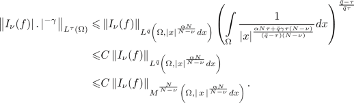 (2.18)
Moreover, combining [28, Theorem 2.4] and [18, Lemma 1.4], we have the following weak type inequality for \(I_\nu \)
$$\begin{aligned} \left\| I_{\nu }(f) \right\| _{M^{\frac{N}{N-\nu }} \left( \Omega , |\,x\,|^{\frac{\alpha N}{N-\nu }} dx \right) } \leqslant C \Vert f |\,.\,|^{\alpha }\Vert _{L^1(\Omega )} \end{aligned}$$(2.19)Therefore, we conclude that
$$\Vert I_{\nu }(f) |\,.\,|^{-\gamma }\Vert _{L^\tau (\Omega )} \leqslant C\, \Vert f |\,.\,|^{\alpha }\Vert _{L^1(\Omega )}$$ - b):
-
The proof in case \(p>1\) is a straight forward consequence of [32, Theorem \(\text {B}^*\)].
\(\square \)
Another integral estimate is necessary and is stated below (see [5, Lemma 3.3] for an elementary proof).
Lemma 2.6
Let \(N \geqslant 1\), \(\rho > 0\) and \(\alpha , \beta \in (-\infty ,N)\). There exists \(C:= C(N,\rho , \alpha , \beta ) > 0\) such that:
-
If \( N-\alpha - \beta \ne 0\), then
$$ \int _{B_\rho (0)} \frac{dz}{|x-z|^{\alpha } |y-z|^{\beta } } \leqslant C \Big (1+ |x-y|^{N-\alpha - \beta } \Big ), \quad \text { for all } x,y \in B_\rho (0) \text { with } x \ne y. $$ -
If \( N - \alpha - \beta = 0\), then
$$ \int _{B_\rho (0)} \frac{dz}{|x-z|^{\alpha } |y-z|^{\beta } } \leqslant C \Big (1+ \big |\ln |x-y|\big | \Big ), \quad \text { for all } x,y \in B_\rho (0)\text { with } x \ne y. $$
Finally, we recall the following interpolation result proven in [33, Theorem 2.9].
Lemma 2.7
Suppose that \(1\leqslant p_1 , p_2 , q_1, q_2 \leqslant \infty \) and
Let \(\Omega \subset \mathbb {R}^N\). Let \(\nu \), \(\mu _1\), \(\mu _2\) and \(\mu \) measures on \(\Omega \) such that \(d\mu _1 = a_1^{p_1} dx\), \(d\mu _2 = a_2^{p_2} dx\) and \(d\mu = a_1^{(1-t)p}a_2^{tp}dx\), where \(a_1, a_2\) are non negative measurable functions.
Assume that T is a linear operator satisfying
and
Then, for all \(0 \leqslant t \leqslant 1\) and \(f\in L^{p}(\Omega ,d\mu )\)
Here \(K_1, K_2\) and \(K_t\) are positive constants independent on f.
3 Regularity results
In this section, we prove Theorem 1.3. As a preliminary step, we state a regularity result for Problem (PH), providing estimates of its solution in weighted Lebesgue spaces.
Theorem 3.1
Let \(0<\lambda <\Lambda _{N}\) and let \(\mu =\mu (\lambda )\) be defined by (1.1). Assume that \(f\in \mathscr {L}^m_{\sigma ,\mu }(\Omega )\) for some \(m\geqslant 1\) and \(\frac{2N\mu }{N-2}\leqslant \sigma \leqslant 2(\mu +1)\). Then if u is the SOLA to (PH), we have:
-
(1)
For \(m=1\), \(\frac{2N\mu }{N-2}\leqslant \beta \leqslant 2(\mu +1)\) and
$$\begin{aligned} \qquad {\left\{ \begin{array}{ll} r= 1 , \qquad & \text{ if } \beta = 2(\mu +1) \\ r\in \left[ 1, \frac{N-\beta }{N-2(\mu +1)}\right) , \qquad & \text{ if } \beta < 2(\mu +1)\,, \end{array}\right. } \end{aligned}$$(3.1)there exists \(C:=C(N, \beta ,\mu ,r,\Omega )>0\) such that
$$\begin{aligned} \left\| u|x|^\mu \right\| _ {M^1\left( \Omega ,|x|^{-\beta }dx\right) } +\left[ 2(\mu +1)-\beta \right] \left\| u|x|^{\mu } \right\| _{L^r(\Omega ,|x|^{-\beta }dx)}\leqslant C\left\| f\right\| _{\mathscr {L}^1_{\sigma ,\mu }(\Omega )}. \end{aligned}$$(3.2) -
(2)
For \(m>1\), \(\frac{2N\mu }{N-2}\leqslant \beta \leqslant 2(\mu +1)\) and
$$\begin{aligned} \qquad {\left\{ \begin{array}{ll} r\in \left[ 1, \frac{m(N-\beta )}{N-\sigma -m(2(\mu +1)-\sigma )}\right) , \qquad & \text{ if } \,1< m<\frac{N-\sigma }{2(\mu +1)-\sigma }\,, \\ r\in [1,+ \infty ), & \text{ if } \ m = \frac{N-\sigma }{2(\mu +1)-\sigma }\,, \\ r=+\infty , & \text{ if } \sigma < 2(\mu + 1) \text { and }\ m >\frac{N-\sigma }{2(\mu +1)-\sigma }\,, \end{array}\right. } \end{aligned}$$(3.3)there exists \(C:=C(N, \sigma , \beta ,\mu ,m,r,\Omega )>0\) such that
$$\begin{aligned} \left\| u|x|^{\mu } \right\| _{L^r(\Omega ,|x|^{-\beta }dx)}\leqslant C\left\| f\right\| _{\mathscr {L}^m_{\sigma ,\mu }(\Omega )}. \end{aligned}$$(3.4)
In [2], the above Theorem was proved for a broader class of Hardy-type operators involving the p-Laplacian, with \(1<p<N\), in the particular case \(\beta =\sigma \). For completeness, and in order to make the present work self-contained, we now provide an elementary proof adapted to the linear case (\(p=2\)), and covering the entire range \(\frac{2N\mu }{N-2}\leqslant \beta \leqslant 2(\mu +1).\)
Proof
Let us set \(v=u|x|^{\mu }\). Hence, According to Proposition 2.4 and (2.15), v is the weak solution to Problem (\(\text {PH}^*\)) with \(h=f|x|^{-\mu }.\) Furthermore,
where \(v_n \in D^{1,2}_{0,\mu }(\Omega )\cap L^\infty (\Omega )\) is the energy solution to the approximating problem

We can assume, without loss of generality , that \({f}\gneqq 0\) (for the general case, apply the result to the positive and negative parts of f). Thus \(v\gneqq 0\) in \(\Omega \).
In the rest of the proof, we denote by C a positive constant that depends only on \(N, \sigma , \beta , \mu , m, r,\) and \(\Omega \), but is independent of n, h, and v. The value of C may change from line to line.
Case 1. \(m=1\):
Let \(k>0\) and let us use \(T_k(v_n)\in D^{1,2}_{0,\mu }(\Omega )\) as a test function in problem (\(\text {PH}^*_n\)). It results that
Using the weighted Caffarelli-Kohn-Nirenberg inequality in Lemma 1.1 and the fact that \(T_k(v_n)\leqslant k\), we get
We deduce that
Therefore, since \(v_n\) converges to v a.e and \(h_n\leqslant h\), we conclude that
Equivalently, we have

In particular, for \(\beta <2(\mu +1)\), we have

Case 2. \(\left\{ \sigma<2(\mu {+}1)~\textrm{and }~1< m<\frac{N-\sigma }{2(\mu {+}1)-\sigma }\right\} ~\textrm{or }~\left\{ \sigma =2(\mu {+}1)~\textrm{and }~1<m<\infty \right\} \)
We define, for \(\frac{2N\mu }{N-2}\leqslant \sigma , \beta \leqslant 2(\mu +1)\)
\(\bullet \) We first assume that \(m\geqslant \frac{2(N-\sigma )}{N+2(\mu +1-\sigma )}\). For a fixed \(\alpha \geqslant 1\) ( to be chosen later), we use \(v_n^\alpha \in D^{1,2}_{0,\mu }(\Omega )\) as a test function in (\(\text {PH}^*_n\)). Then it follows that
Hence
Using the weighted Caffarelli-Kohn-Nirenberg inequality in Lemma 1.1, we get
Now, using Hölder’s inequality, it holds that
We shall prove that
We proceed by considering the following three cases individually:
If \(\beta =\sigma \), then choosing \(\alpha = \frac{(m-1)(N-\sigma )}{N-\sigma -m(2(\mu +1)-\sigma )}\geqslant 1 \), we reach that for all \(n\geqslant 1\),
Next, if \(\beta > \sigma \), then by a straightforward application of Hölder’s inequality together with (3.11), we obtain that for all \(1 \leqslant r< \overline{r}\left( \sigma ,\beta \right) \), there exists a positive constant \(C=C\left( \Omega ,\beta ,\sigma , r, m, N, \mu \right) \), such that
Finally, in the case \(\beta < \sigma \), we choose any \( 1 \leqslant \alpha < \frac{(m-1)(N-\sigma )}{\,N - \sigma - m(2(\mu +1)-\sigma )\,}. \) Then, applying Hölder’s inequality once again, we deduce that
Thus, for every \( 1 \leqslant \alpha < \frac{(m-1)(N-\sigma )}{\,N - \sigma - m(2(\mu +1)-\sigma )\,} \), we obtain
Equivalently, for all \(1 \leqslant r< \overline{r}\left( \sigma ,\beta \right) \), we have
Then, claim (3.10) is established. Now, using Fatou’s lemma and the fact that \( h_n\leqslant h\), we get
\(\bullet \) Regarding the case \(1<m< \frac{2(N-\sigma )}{N+2(\mu +1-\sigma )}\), we will use an interpolation argument. For this, we define the solution map to problem (\(\text {PH}^*\))

Given estimates (3.7) and (3.16) above, there exist positive constants \(K_1\) and \(K_2\) , independent on h, such that
and
where \(p_1=1,\, p_2= \frac{2(N-\sigma )}{N+2(\mu +1-\sigma )},\, q_1= \frac{N-\beta }{N-2(\mu +1)} \) and \(\, q_2\in \left[ 1,\frac{2(N-\beta )}{N-2(\mu +1)}\right) \).
Therefore, since \(\dfrac{1}{m} = \dfrac{1-t}{p_1}+ \dfrac{t}{p_2}\) for some \(t\in (0,1)\), applying Lemma 2.7, we reach that
Case 3. \( \left\{ \sigma <2(\mu +1) \text { and } m=\frac{N-\sigma }{2(\mu +1)-\sigma }\right\} \text { or } \left\{ \sigma =2(\mu +1) \text { and } m=\infty \right\} \) :
This case is a simple consequence of the previous case.
Case 4. \( \sigma <2(\mu +1) \text { and } m>\frac{N-\sigma }{2(\mu +1)-\sigma }\) :
Let \(k>0\), then, using \(G_k(v_n)\) as a test function in (\(\text {PH}^*_n\)), it follows that
Thus, using the Hölder inequality, we get
Now, by the Caffarelli-Kohn-Nirenberg inequality in Lemma 1.1, we deduce that
Hence, for all \(l>k\)
Thus, since \(m>\frac{N-\sigma }{2(\mu +1)-\sigma }\), using the standard Stampacchia argument, see [30], we get the existence of a positive constant (independent on n)
such that
Hence \( \big |\{x\in \Omega : v(x)\geqslant k_0\}\big |=0\) and consequently \(v\in L^\infty (\Omega )\). Furthermore,
Finally, expressing the estimates in terms of u and f in all cases, concludes the proof. \(\square \)
We now proceed to the proof of Theorem 1.3.
Proof of Theorem 1.3
Let u be the SOLA to problem (PH). Then, thanks to the representation formula (2.4), we obtain
Now, applying Lemma 2.1, we infer
In the remainder of the proof, C denotes a positive constant that depends only on \(N, \sigma , \beta , \mu , m, r,\) and \(\Omega \), but is independent of u and f. Its value may change from line to line.
We consider 4 cases separately
Case 1. \(m=1\) :
\(\bullet \) Let \(\frac{N(2\mu +1)}{N-1}\leqslant \beta < 2(\mu +1)\) and \(1\leqslant r< \frac{(N-\beta )}{N-2(\mu +1)}\). Hence
We start by estimating \(J_1\). Since \(\Omega \) is bounded, we may assume that
Considering the parameters
and observing that
we deduce, from Proposition 2.5 and Theorem 3.1, that
On the other hand, for
one easily checks that
Therefore, applying Proposition 2.5, we obtain
Consequently, having at hand (3.19), (3.21), (3.24), it follows that
\(\bullet \) Next, let \(\beta = 2(\mu +1)\) and let \(l>0\) and \(k>0\).
First, it follows from (3.2) that
On the other hand, since
then,
Applying (3.2), we reach that
Moreover, using estimate (2.11), we obtain
Combining (3.26)-(3.30), we get
Thus, choosing \(k=l\), we have
Therefore, we conclude that
Case 2. \( \left\{ \sigma<2(\mu +1) \text { and } 1< m<\frac{N-\sigma }{2(\mu +1)-\sigma }\right\} \text { or } \left\{ \sigma =2(\mu +1) \text { and } 1<m<\infty \right\} \) :
We define, for \(\frac{N(2\mu +1)}{N-1}\leqslant \sigma , \beta \leqslant 2(\mu +1)\)
Let \(1 \leqslant r < \overline{r}(\sigma ,\beta )\). Thus,
First, following exactly the same argument used for \(J_1\) above, we obtain
Secondly, let us take
Note that
Then the assumptions of Proposition 2.5 are satisfied. Applying the proposition yields
Hence, combining (3.33), (3.34) and (3.37), it follows that
Case 3. \( \left\{ \sigma <2(\mu +1) \text { and } m=\frac{N-\sigma }{2(\mu +1)-\sigma }\right\} \text { or } \left\{ \sigma =2(\mu +1) \text { and } m=\infty \right\} \) :
Let \(1\leqslant r< \infty \), then there exists \(m_1\in \left( 1,m\right) \) close enough to m ( or large enough if \(m=\infty \)) such that
Thus, thanks to the result in the previous case and Hölder inequality, it holds that
Case 4. \( \sigma <2(\mu +1) \text { and } m>\frac{N-\sigma }{2(\mu +1)-\sigma }\) :
For \(x\in \Omega \)
First, by applying Theorem 3.1 followed by Lemma 2.6, we obtain
Secondly, using Hölder’s inequality and then Lemma 2.6, we get
Therefore, since \(m>\frac{N-\sigma }{2(\mu +1)-\sigma }\), then
We conclude from (3.40), (3.41) and (3.42) that
\(\square \)
Assume that \(f\in \mathscr {L}^m_{\sigma ,\mu }(\Omega )\) for some \(m\geqslant 1\) and \(\frac{2N\mu }{N-2}\leqslant \sigma \leqslant 2(\mu +1)\). We emphasize that the parameter \(\beta \) appearing in Theorems 3.1 and 1.3 is independent of \(\sigma \) and m. In particular, \(\beta \) will be chosen so as to interpret the above results as \(D^{1,p}_{0,t}(\Omega )\)-type regularity for the solution u to (PH). As a consequence, we obtain the following corollary.
Corollary 3.2
Let \(0<\lambda <\Lambda _{N}\) and let \(\mu =\mu (\lambda )\) be defined by (1.1). Assume that \(f\in \mathscr {L}^1_{\sigma ,\mu }(\Omega )= L^1(\Omega ,|x|^{-\mu }dx)\) and let u be the SOLA to problem (PH). Then,
-
(1)
$$\begin{aligned} u|x|^{-\mu } \in L^\theta (\Omega ), \quad \forall \ \theta \in \left[ 1, \frac{N}{N-2} \right) \end{aligned}$$(3.44)
and
$$\begin{aligned} \nabla u|x|^{-\mu } \in L^p(\Omega ), \quad \forall \ p \in \left[ 1, \frac{N}{N-1} \right) . \end{aligned}$$(3.45)In particular, there exists \(C := C(N,\theta ,p,\Omega ,\mu )> 0\) such that
$$\begin{aligned} \left\| u |x|^{-\mu }\right\| _{L^{\theta }(\Omega )}+\left\| \nabla u |x|^{-\mu }\right\| _{L^{p}(\Omega )}\leqslant C\, \left\| f\right\| _{L^1(\Omega ,|x|^{-\mu }dx)}\,. \end{aligned}$$(3.46)Moreover, the solution map
$$ \mathbb {S}_\mu : L^1(\Omega ,|x|^{-\mu } dx) \rightarrow D_{0,\mu }^{1,p}(\Omega ), \quad f \mapsto \mathbb {S}[f] := u $$is well-defined, continuous and compact.
-
(2)
If \(f\in \mathscr {L}^m_{\sigma ,\mu }(\Omega )\) for some \(m\geqslant 1\) and \(\frac{2N\mu }{N-2}\leqslant \sigma \leqslant 2(\mu +1)\). Then, for
$$\begin{aligned} \qquad {\left\{ \begin{array}{ll} \theta \in \left[ 1, \dfrac{N}{N-2} \right) , & \text{ if } m=1,\\ \theta \in \left[ 1, \dfrac{mN}{N-2} \dfrac{N- 2(\mu +1)}{N-\sigma -m(2(\mu +1)-\sigma )} \right) ,\qquad \qquad & \text{ if } 1< m<\frac{N-\sigma }{2(\mu +1)-\sigma }\,, \\ \theta \in [1, \infty ), & \text{ if } \ m = \frac{N-\sigma }{2(\mu +1)-\sigma }\,,\\ \theta =\infty , & \text{ if } \sigma < 2(\mu + 1) \text { and } \\ & \quad m >\frac{N-\sigma }{2(\mu +1)-\sigma }\,, \end{array}\right. } \end{aligned}$$(3.47)there exists \(C := C(N,\theta ,\Omega ,\mu , \sigma , m)> 0\) such that
$$\begin{aligned} \left\| u |x|^{-s}\right\| _{L^{\theta }(\Omega )}\leqslant C\, \left\| f\right\| _{\mathscr {L}^m_{\sigma ,\mu }(\Omega )}\,, \end{aligned}$$(3.48)where
$$\begin{aligned} s= {\left\{ \begin{array}{ll} \mu , & \qquad \qquad \text { if } m=1,\\ \mu \left[ \dfrac{2(N-\sigma ) -m\left( N+2\left( \mu +1-\sigma \right) \right) }{m\left( N-2\left( \mu +1\right) \right) }\right] , & \qquad \qquad \text { if } \; 1< m < \frac{N-\sigma }{2(\mu +1)-\sigma },\\ -\mu , & \qquad \qquad \text { if } \; m \geqslant \frac{N-\sigma }{2(\mu +1)-\sigma }. \end{array}\right. } \end{aligned}$$(3.49) -
(3)
If \(f\in \mathscr {L}^m_{\sigma ,\mu }(\Omega )\) for some \(m\geqslant 1\) and \(\frac{N(2\mu +1)}{N-1}\leqslant \sigma \leqslant 2(\mu +1)\). Then, for
$$\begin{aligned} \qquad {\left\{ \begin{array}{ll} p\in \left[ 1, \dfrac{N}{N-1} \right) , & \text{ if } m=1,\\ p\in \left[ 1, \dfrac{mN}{N-1} \dfrac{N- 2(\mu +1)}{N-\sigma -m(2(\mu +1)-\sigma )} \right) ,\qquad \qquad & \text{ if } 1< m<\frac{N-\sigma }{2(\mu +1)-\sigma }\,, \\ p\in [1, \infty ), & \text{ if } \ m = \frac{N-\sigma }{2(\mu +1)-\sigma }\,,\\ p=\infty , & \text{ if } \sigma < 2(\mu + 1) \\ & \quad \text { and } \ m >\frac{N-\sigma }{2(\mu +1)-\sigma }\,, \end{array}\right. } \end{aligned}$$(3.50)there exists \(C := C(N,p,\Omega ,\mu , \sigma , m)> 0\) such that
$$\begin{aligned} \left\| \nabla u |x|^{-t}\right\| _{L^{p}(\Omega )}\leqslant C\, \left\| f\right\| _{\mathscr {L}^m_{\sigma ,\mu }(\Omega )}\,, \end{aligned}$$(3.51)where
$$\begin{aligned} t= {\left\{ \begin{array}{ll} \mu , & \qquad \qquad \text { if } m=1, \\ s- \dfrac{(m-1)(N-\sigma ) }{m\left( N-2\left( \mu +1\right) \right) }, \qquad & \qquad \qquad \text { if } \; 1< m < \frac{N-\sigma }{2(\mu +1)-\sigma },\\ -(\mu +1), \qquad & \qquad \qquad \text { if } \; m \geqslant \frac{N-\sigma }{2(\mu +1)-\sigma }. \end{array}\right. } \end{aligned}$$(3.52)
Proof
-
(1)
Assume that \(f\in \mathscr {L}^1_{\sigma ,\mu }(\Omega )= L^1(\Omega ,|x|^{-\mu }dx)\). First, observe that estimate (3.46) is a consequence of the combination of (3.2) and (1.7). Indeed, for \(\beta = \frac{2N\mu }{N-2}\) and for all \(1\leqslant \theta <\frac{N}{N-2}\), we have
$$ \left\| u|x|^{-\mu }\right\| _{L^\theta (\Omega )}\leqslant C_1 \left\| u|x|^{\mu } \right\| _{L^\theta (\Omega ,|x|^{-\beta }dx)} , \quad \text { where } C_1:= {{\,\textrm{diam}\,}}(\Omega )^\frac{\beta - 2\mu \theta }{\theta }. $$Moreover, for all \(\frac{2N\mu }{N-2}\leqslant \beta < 2(\mu +1)\), \(1\leqslant r<\frac{N-\beta }{N-2(\mu +1)},\) and \(\frac{rN}{N-\beta +2\mu r}<\theta < \frac{N}{N-2}\), we infer that
$$\begin{aligned}&\left\| u|x|^{\mu } \right\| _{L^r(\Omega ,|x|^{-\beta }dx)}\leqslant C_2 \left\| u|x|^{-\mu }\right\| _{L^\theta (\Omega )}, \\ &\quad \text { where } C_2:= \left( \int _{\Omega }\frac{1}{|x|^{\frac{(\beta -2\mu r)\theta }{\theta -r}}} dx\right) ^{\frac{\theta -r}{r\theta }}. \end{aligned}$$On the other hand, for \( \beta =\frac{N(2\mu +1)}{N-1}\) and for all \(1\leqslant p <\frac{N}{N-1}\), we have
$$\begin{aligned} \left\| \nabla u|x|^{-\mu }\right\| _{L^p(\Omega )}\leqslant C_1\left\| \nabla u|x|^{\mu +1} \right\| _{L^p(\Omega ,|x|^{-\beta }dx)} , \quad \text { where } C_1:= {{\,\textrm{diam}\,}}(\Omega )^\frac{\beta -p(2\mu +1)}{p}. \end{aligned}$$Furthermore, for all \(\frac{N(2\mu +1)}{N-1}\leqslant \beta < 2(\mu +1)\), \(1\leqslant r<\frac{N-\beta }{N-2(\mu +1)},\) and \(\frac{rN}{N-\beta + r(2\mu +1) }<p< \frac{N}{N-1}\), we get
$$\begin{aligned} \left\| \nabla u|x|^{\mu +1} \right\| _{L^r(\Omega ,|x|^{-\beta }dx)} \leqslant C_2 \left\| \nabla u|x|^{-\mu }\right\| _{L^p(\Omega )},\text { where } C_2:= \left( \int _{\Omega }\frac{1}{|x|^{\frac{(\beta -r(2\mu +1) )p}{p-r}}} dx\right) ^{\frac{p-r}{rp}}. \end{aligned}$$The estimates above show, in particular, that the solution map \(\mathbb {S}_\mu \) is well defined and continuous from \(L^1(\Omega ,|x|^{-\mu } dx)\) to \(D_{0,\mu }^{1,p}(\Omega )\) for all \(1 \leqslant p < \frac{N}{N-1}\). We prove next that it is compact as well. Let \(\left( f_n\right) _n \) be a bounded sequence in \(L^1(\Omega ,|x|^{-\mu } dx)\) and let \(u_n =\mathbb {S}_\mu (f_n)\) for all \(n\in \mathbb {N}\). First, according to (3.46), we know that
$$\begin{aligned} \left( u_n |x|^{-\mu }\right) _n \text { is bounded in } L^\theta (\Omega ), \quad \forall \ \theta \in \left[ 1, \frac{N}{N-2} \right) \end{aligned}$$and
$$\begin{aligned} \left( \nabla \left( u_n\right) |x|^{-\mu }\right) _n \text { is bounded in } L^p(\Omega ), \quad \forall \ p \in \left[ 1, \frac{N}{N-1} \right) .\end{aligned}$$Additionally, it is easy to see that
$$ \left( \lambda \frac{u_n}{|x|^2}+ f_n \right) _n \text { is bounded in } L^1(\Omega ),$$which implies, according to the compactness result in Proposition 2.2, that there exists \(u \in W^{1,p}_{0} (\Omega )\) such that, up to a subsequence,
$$\begin{aligned} u_n \underset{n\longrightarrow \infty }{\longrightarrow }\ u , \quad \text { a.e. on } \Omega , \qquad \qquad \nabla u_n \underset{n\longrightarrow \infty }{\longrightarrow }\ \nabla u , \quad \text { a.e. on } \Omega \end{aligned}$$and
$$\begin{aligned} u_n \underset{n\longrightarrow \infty }{\longrightarrow }\ u \text { in } W^{1,p}_{0} (\Omega ), \quad \forall \ p \in \left[ 1, \frac{N}{N-1} \right) . \end{aligned}$$Thus, using Vitali convergence’s theorem we deduce that
$$\begin{aligned} u_n \underset{n\longrightarrow \infty }{\longrightarrow }\ u \text { in }D_{0,\mu }^{1,p}(\Omega ), \quad \forall \ p \in \left[ 1, \frac{N}{N-1} \right) . \end{aligned}$$ -
(2)
Assume that \(f\in \mathscr {L}^m_{\sigma ,\mu }(\Omega )\) for some \(m\geqslant 1\) and \(\frac{2N\mu }{N-2}\leqslant \sigma \leqslant 2(\mu +1)\). We focus on the case \(1< m<\frac{N-\sigma }{2(\mu +1)-\sigma }\), the remaining cases being treated before. For s defined by (3.49), \(\beta = \frac{2N\mu }{N-2}\) and for all \(1\leqslant \theta <\frac{mN}{N-2} \frac{N- 2(\mu +1)}{N-\sigma -m(2(\mu +1)-\sigma )}, \) we have
$$\begin{aligned} \left\| u|x|^{-s}\right\| _{L^\theta (\Omega )}\leqslant C_1 \left\| u|x|^{\mu } \right\| _{L^\theta (\Omega ,|x|^{-\beta }dx)} , \quad \text { where } C_1:= {{\,\textrm{diam}\,}}(\Omega )^\frac{\beta -\theta (\mu +s)}{\theta }. \end{aligned}$$Furthermore, for all \(\frac{2N\mu }{N-2}\leqslant \beta \leqslant 2(\mu +1)\), \(1\leqslant r<\frac{m(N-\beta )}{N-\sigma -m(2(\mu +1)-\sigma )},\) and \(\frac{rN}{N-\beta +r\left( s+\mu \right) }<\theta < \frac{mN}{N-2} \frac{N- 2(\mu +1)}{N-\sigma -m(2(\mu +1)-\sigma )}\), we obtain that
$$\begin{aligned} \left\| u|x|^{\mu } \right\| _{L^r(\Omega ,|x|^{-\beta }dx)}\leqslant C_2 \left\| u|x|^{-s}\right\| _{L^\theta (\Omega )}, \quad \text { where } C_2 := \left( \int _{\Omega }\frac{1}{|x|^{\frac{\left( \beta - r\left( s+\mu \right) \right) \theta }{\theta -r}}} dx\right) ^{\frac{\theta -r}{r\theta }}. \end{aligned}$$ -
(3)
Assume that \(f\in \mathscr {L}^m_{\sigma ,\mu }(\Omega )\) for some \(m\geqslant 1\) and \(\frac{N(2\mu +1)}{N-1}\leqslant \sigma \leqslant 2(\mu +1)\). It remains to consider the range \(1< m<\frac{N-\sigma }{2(\mu +1)-\sigma }\). For t defined by (3.52), \(\beta =\frac{N(2\mu +1)}{N-1}\) and for all \(1\leqslant p <\frac{mN}{N-1} \frac{N- 2(\mu +1)}{N-\sigma -m(2(\mu +1)-\sigma )}, \) we have
$$\begin{aligned} \left\| \nabla u|x|^{-t}\right\| _{L^p(\Omega )}\leqslant C_1\left\| \nabla u|x|^{\mu +1} \right\| _{L^p(\Omega ,|x|^{-\beta }dx)} , \quad \text { where } C_1 := {{\,\textrm{diam}\,}}(\Omega )^\frac{\beta -p(\mu +1+t)}{p} . \end{aligned}$$Also, for all \(\frac{N(2\mu +1)}{N-1}\leqslant \beta \leqslant 2(\mu +1)\), \(1\leqslant r<\frac{m(N-\beta )}{N-\sigma -m(2(\mu +1)-\sigma )},\) and \(\frac{rN}{N-\beta +r\left( t+\mu +1 \right) }<p< \frac{mN}{N-1} \frac{N- 2(\mu +1)}{N-\sigma -m(2(\mu +1)-\sigma )}\), we reach that
$$\begin{aligned}&\left\| \nabla u|x|^{\mu +1} \right\| _{L^r(\Omega ,|x|^{-\beta }dx)}\leqslant C_2 \left\| \nabla u|x|^{-t}\right\| _{L^p(\Omega )},\\&\quad \text { where } C_2:= \left( \int _{\Omega }\frac{1}{|x|^{\frac{\left( \beta -r\left( t+\mu +1 \right) \right) p}{p-r}}} dx\right) ^{\frac{p-r}{rp}}. \end{aligned}$$
This ends our proof. \(\square \)
4 Application: Hardy-KPZ problem
By means of the regularity results from the previous section, we establish in this section Theorem 1.2, which guarantees the existence of a weak solution for problem (KPZH).
Proof of Theorem 1.2
Assume that \(f\in \mathscr {L}^m_{\sigma ,\mu }(\Omega )\) where \(\sigma =\frac{N(2\mu +1)}{N-1}\) and \(m\geqslant 1\).
The proof is divided into cases according to the values of m (we closely adapt the arguments from [6] ).
Case 1: \(1\leqslant m < \frac{N-\sigma }{2(\mu +1)-\sigma } = N\).
Let \(t\in \mathbb {R}\) be the parameter defined in (3.52). Hence,
Also, let
and choose \(r>1\), satisfying
Define
where K is a positive constant that will be specified later in (4.11).
Since \(q > 1\), we know from [4, Lemma 4.1], that there exists a unique \(\ell \in (0,\infty )\) such that
Having at hand \(\rho ^{\star }\) and \(\ell \), we define
which is easily seen to be closed and convex in \(D^{1,1}_{0,\mu }(\Omega )\). Furthermore, observe that, for all \(v\in E_1\)
where
Hence, in view of the continuous embedding \(L^q(\Omega ,|x|^{-\mu }dx) \hookrightarrow L^1(\Omega ,|x|^{-\mu }dx)\), it follows immediately that \(E_1\) is bounded in \(D^{1,1}_{0,\mu }(\Omega )\).
We shall prove the existence of a weak solution to (KPZH) belonging to \(E_1\) using Schauder’s fixed-point theorem. Let us consider
where u is the unique SOLA of the following problem
As a consequence of (4.6) and Corollary 3.2 (1), the operator \(F_1\) is well defined on \(E_1\). The existence of a solution will follow once we establish that \(F_1\) admits a fixed point in \(E_1\). It remains to verify that \(F_1\) is continuous and compact, and that \(F_1(E_1) \subset E_1\) for \(0<\rho \leqslant \rho ^{\star }\).
We first show that \(F_1(E_1) \subset E_1\) for \(0<\rho \leqslant \rho ^{\star }\). For this, take \(v \in E_1\) and set \(u = F_1(v)\). Thanks to Corollary 3.2 (3), there exists \(K_1 := K_1(N,r,\Omega ,\mu , \sigma , m)> 0\), such that
where \(K_2\) is defined by (4.7) and
Hence, it follows from (4.4), that
Therefore, \(F_1(E_1) \subset E_1\).
We now show that \(F_1\) is compact. Let \(\left( v_n\right) _n \subset E_1\) with \(\Vert v_n\Vert _{D^{1,1}_{0,\mu }(\Omega )} \leqslant 1\) for all \(n \in \mathbb {N}\), and define \(h_n := |\nabla v_n|^q + \rho f\). Clearly, \(\left( h_n\right) _n\) is bounded in \(L^1(\Omega , |x|^{-\mu } dx)\). The compactness of \(F_1\) then follows directly from Corollary 3.2 (1).
Finally, we establish the continuity of \(F_1\). Let \(\left( v_n\right) _n \subset E_1\) be a sequence such that \(v_n \rightarrow v\) in \(D^{1,1}_{0,\mu }(\Omega )\) and set \(u_n = F_1(v_n)\) for all \(n \in \mathbb {N}\) and \(u = F_1(v)\). Note that
If one shows that the right-hand side in (4.12) converges to 0 in \(L^1(\Omega ,|x|^{-\mu }dx)\) as \(n \rightarrow \infty \), then the continuity of \(F_1\) follows directly from Corollary 3.2 (1). Consequently, the solution, in the case \( 1 \leqslant m <N\), will be obtained. By applying the Mean Value Theorem, then Hölder’s inequality, we have that
where \(\widetilde{K}\) is given in (4.6). Moreover, employing interpolation in \(L^p\)–spaces, we deduce that
with \(1<q<\kappa <r\) and \(\frac{1}{q} = \theta +\frac{1-\theta }{\kappa }\). Thus, in view of (4.6), choosing \(\kappa \) sufficiently close to q ensures the existence of a positive constant \(\overline{K}:= \overline{K}(N,r, \kappa , \Omega , \mu , m, \ell )\), such that
Finally, given that \(v_n \rightarrow v\) in \( D^{1,1}_{0,\mu }(\Omega )\), combining (4.13) and (4.15), we conclude that
which completes the argument. As a result, the existence of a weak solution to (KPZH) in the case \(1\leqslant m < N\) is proven. Moreover, the regularity of the solution obtained is a simple consequence of Corollary 3.2.
Case 2: \(m \geqslant \frac{N-\sigma }{2(\mu +1)-\sigma }= N\).
First of all, observe that, since \(\Omega \) is bounded we can assume (without loss of generality) that \( m = N\). Then, for \(1<q<\overline{q}=\frac{\mu +2}{\mu +1}\), let us choose \(r\in (1,\infty )\) such that
and define
where \(C>0\) is a positive constant given later in (4.25).
For \(q>1\), [4, Lemma 4.1] guarantees the existence of a unique \(\ell \in (0,\infty )\) such that
Given \(\rho ^{\star }\) and \(\ell \), we introduce the set
and point out that \(E_2\) is a closed and convex subset of \(D^{1,1}_{0,\mu }(\Omega )\). We also note that for all \(v \in E_2\),
where
Consequently, by the continuous embedding \( L^q(\Omega ,|x|^{-\mu }dx) \hookrightarrow L^1(\Omega ,|x|^{-\mu }dx), \) we reach that \(E_2\) is bounded in \(D^{1,1}_{0,\mu }(\Omega )\).
The existence of a weak solution to (KPZH) in \(E_2\) follows by a further application of Schauder’s fixed point theorem, as in Case 1. Let us consider
where u is the unique SOLA of the following problem
It suffices to show that the operator \(F_2\) admits a fixed point in \(E_2\), since this directly yields the existence of a solution. By (4.20) and Corollary 3.2 (1), the operator \(F_2\) is well defined on \(E_2\). Therefore, to conclude the proof in this case, it remains to verify the invariance property \( F_2(E_2) \subset E_2, \) as the continuity and compactness of \(F_2\) follow exactly as in the proof for \(F_1\).
Let \(0<\rho \leqslant \rho ^{\star }\), \(v \in E_2\) and \(u = F_2(v)\). As a consequence of Corollary 3.2 (3), there exists a constant \(C_1 := C_1(N,r,\Omega ,\mu ,\sigma ) > 0\) such that
where \(C_2\) is defined by (4.21) and
In view of (4.18), we obtain
This shows that the operator \(F_2\) maps \(E_2\) into itself, namely \(F_2(E_2) \subset E_2\).
Finally, the regularity of the solution follows once more as a direct consequence of Corollary 3.2. This settles the case \(m \geqslant N\) and completes the proof of the result. \(\square \)
5 Further results and perspectives
\(\bullet \) The results obtained in this paper can be useful for studying the nonlocal version of (KPZH), namely
where \(s \in (0,1)\) and \(0<\lambda \leqslant \Lambda _{N,s}:= 2^{2s}\frac{\Gamma ^2(\frac{N+2s}{4})}{\Gamma ^2(\frac{N-2s}{4})}\). Here \((-\Delta )^s\) denotes the fractional Laplacian, while \(D^s\) stands for one of the following nonlocal gradients:
where \(\alpha _{N,\sigma }\) and \(\beta _{N,\sigma }\) are normalization constants and “P.V.” stands for “in the principal value sense”. We refer to [6] for further details and related literature on these nonlocal gradients. As in the local case, the presence of the Hardy potential introduces two characteristic exponents associated with the homogeneous equation
More precisely, for every \(0<\lambda \leqslant \Lambda _{N,s}\), there exist two positive constants
such that the radial functions
solve (5.2) in the distributional sense. See [1] for the explicit characterization of \(\mu (\lambda )\) and \(\bar{\mu }(\lambda )\).
In particular, the authors of [1] raised several questions concerning problems of the form (5.1), and we believe that they can be addressed using the approach developed in the present paper. For instance, nonexistence results are known when \( q\geqslant q^+ := \frac{\mu +2s}{\mu +s}, \) whereas the existence of a weak solution for \(1<q<q^+\) and sufficiently small \(\rho >0\) remains, to our knowledge, an open problem.
\(\bullet \) We point out that for nonlinear operators the situation is more delicate. In particular, for the p-Laplacian, the transformation (\(v=|x|^\mu u\)), which plays a crucial role in the proof of Theorem 3.1, is no longer available due to the nonlinear nature of the operator. Moreover, the weighted regularity estimates established in Theorem 1.3 rely on the linear representation formula and on weighted integral estimates. For the Poisson problem driven by the p-Laplacian, such tools are not available in the same form, making the analysis substantially more difficult. Although important results have been obtained through nonlinear potential theory and Wolff potential estimates, the regularity theory remains far from being as complete as in the linear case.
Data Availability
No datasets were generated or analysed during the current study.
References
Abdellaoui, B., Biroud, K., Primo, A., Soria, F., Younes, A.: Fractional KPZ equations with fractional gradient term and Hardy potential. Math. Eng 5(2), 1–36 (2023)
Abdellaoui, B., Colorado, E., Sanchón, M.: Regularity of entropy solutions of quasilinear elliptic problems related to Hardy-Sobolev inequalities. Adv. Nonlinear Stud. 6(4), 547–562 (2006)
Abdellaoui, B., Dall’Aglio, A., Peral, I.: Some remarks on elliptic problems with critical growth in the gradient. J. Differ. Equ. 222(1), 21–62 (2006)
Abdellaoui, B., Fernández, A.J.: Nonlinear fractional Laplacian problems with nonlocal ’gradient terms. Proc. R. Soc. Edinb. A: Math 150(5), 2682–2718 (2020)
Abdellaoui, B., Fernández, A.J., Leonori, T., Younes, A.: Global fractional Calderón–Zygmund-type regularity. Commun. Contemp. Math. 27(8), 2550004 (2024)
Abdellaoui, B., Fernández, A.J., Leonori, T., Younes, A.: Deterministic KPZ-type equations with nonlocal “gradient terms’’. Annali di Matematica 202(3), 1451–1468 (2023)
Abdellaoui, B., Peral, I.: Some results for semilinear elliptic equations with critical potential. Proc. R. Soc. Edinb. A: Math 132(1), 1–24 (2002)
Abdellaoui, B., Peral, I.: On quasilinear elliptic equations related to some Caffarelli-Kohn-Nirenberg inequalities. Commun. Pure Appl. Anal. 2(4), 539–566 (2003)
Abdellaoui, B., Peral, I.: A note on a critical problem with natural growth in the gradient. J. Eur. Math. Soc. 8(2), 157–170 (2006)
Abdellaoui, B., Peral, I.: The equation \(-\Delta {u}-\lambda \dfrac{{u}}{|{x}|^{ 2}}=|\nabla {u}|^{{p}}+{c}{f}({x}) \): The optimal power. Annali della Scuola Normale Superiore di Pisa-Classe di Scienze 6(1), 159–183 (2007)
Abdellaoui, B., Peral, I., Primo, A.: Elliptic problems with a Hardy potential and critical growth in the gradient: non-resonance and blow-up results. J. Differ. Equ. 239(2), 386–416 (2007)
Alaa, N.E., Pierre, M.: Weak solutions of some quasilinear elliptic equations with data measures. SIAM J. Math. Anal. 24(1), 23–35 (1993)
Boccardo, L., Gallouët, T.: Non-linear elliptic and parabolic equations involving measure data. J. Funct. Anal. 87(1), 149–169 (1989)
Boccardo, L., Murat, F., Puel, J.P.: Existence de solutions non bornées pour certaines équations quasi-linéaires Port. Math. 41(1–4), 507–534 (1982)
Boccardo, L., Murat, F., Puel, J.P.: Résultats d’existence pour certains problèmes elliptiques quasilinéaires. Annali della Scuola Normale Superiore di Pisa-Classe di Scienze 11(2), 213–235 (1984)
Boccardo, L., Orsina, L., Peral, I.: A remark on existence and optimal summability of solutions of elliptic problems involving Hardy potential. Discrete Contin. Dynam. Systems 3, 513–523 (2006)
Brezis, H., Dupaigne, L., Tesei, A.: On a semilinear elliptic equation with inverse-square potential. Sel. Math. New Ser. 11(1), 1–7 (2005)
Buckley, S.M.: Estimates for operator norms on weighted spaces and reverse Jensen inequalities. Trans. Am. Math. Soc. 340(1), 253–272 (1993)
Caffarelli, L., Kohn, R., Nirenberg, L.: First order interpolation inequalities with weights. Compos. Math. 53(3), 259–275 (1984)
Chen, H., Quaas, A., Zhou, F.: On nonhomogeneous elliptic equations with the Hardy-Leray potentials. Journal d’Analyse Mathématique 144(1), 305–334 (2021)
Chen, H., Véron, L.: Boundary singularities of semilinear elliptic equations with Leray-Hardy potential. Commun. Contemp. Math. 24(07), 2150051 (2022)
Chen, H., Véron, L.: Weak solutions of semilinear elliptic equations with Leray-Hardy potential and measure data. Math. Eng 1(3), 391–418 (2019)
Chen, Z.Q., Wang, J.M.: Green function estimates for second order elliptic operators in non-divergence form with Dini continuous coefficients. Electron. J. Probab. 28, 1–54 (2023)
Dupaigne, L.: A nonlinear elliptic PDE with the inverse-square potential. Journal d’Analyse Mathématique 86(1), 359–398 (2002)
Ferone, V., Murat, F.: Quasilinear problems having natural growth in the gradient: an existence result when the source term is small. In: Équations aux dérivées partielles et applications. Articles dédiés à Jacques-Louis Lions Gauthier-Villars, Éditions Scientifiques et Médicales, pp. 497–515. Elsevier (1998)
Hansson, K., Maz’ya, V.G., Verbitsky, I.E.: Criteria of solvability for multidimensional Riccati equations. Arkiv för Matematik 37(1), 87–120 (1999)
Krasnoselskii, M.A., Zabreiko, P.P., Pustylnik, E.I., Sobolevskii, P.E.: Integral operators in spaces of summable functions,, Noordhoff (1966)
Lacey, M.T., Moen, K., Pérez, C., Torres, R.H.: Sharp weighted bounds for fractional integral operators. J. Funct. Anal. 259(5), 1073–1097 (2010)
Porzio, M.M.: On some quasilinear elliptic equations involving Hardy potential. Rendiconti di Matematica e delle sue Applicazioni, Serie VII 27(3–4), 277–299 (2007)
Stampacchia, G.: Le problème de Dirichlet pour les équations elliptiques du second ordre à coefficients discontinus. In Annales de l’institut Fourier. 15(1), 189–257 (1965)
Stein, E.M.: Singular integrals and differentiability properties of functions. Princeton University Press, Princeton, NJ (1970)
Stein, E.M., Weiss, G.: Fractional integrals on n-dimensional Euclidean space. J. Appl. Math. Mech. 7(4), 503–514 (1958)
Stein, E.M., Weiss, G.: Interpolation of operators with change of measures. Trans. Am. Math. Soc. 87(1), 159–172 (1958)
Véron, L.: Elliptic equations involving measures. In Handbook of differential equations: Stationary partial differential equations 1, 593–712 (2004). (North-Holland)
Acknowledgements
Part of this work was carried out while the second and the fourth authors were visiting the Department of Mathematics at the University Autonoma of Madrid. They would like to express their sincere gratitude for the warm hospitality of the department. The authors would also like to thank the anonymous referee for the careful reading of the manuscript and for the valuable comments and suggestions, which helped improve the quality and clarity of the paper.
Funding
Open Access funding provided thanks to the CRUE-CSIC agreement with Springer Nature. Work partially supported by Project PID2023-150166NB-100, MINECO, Spain. The work is also supported by Erasmus type project between the Autonoma university and the Aboubekr Belkaid university of Tlemcen.
Author information
Authors and Affiliations
Contributions
All authors wrote and reviewed the manuscript.
Corresponding author
Ethics declarations
Conflicts of Interest
The authors state no conflict of interest.
Additional information
Publisher's Note
Springer Nature remains neutral with regard to jurisdictional claims in published maps and institutional affiliations.
Work partially supported by Project PID2023-150166NB-100, MINECO, Spain.
Rights and permissions
Open Access This article is licensed under a Creative Commons Attribution 4.0 International License, which permits use, sharing, adaptation, distribution and reproduction in any medium or format, as long as you give appropriate credit to the original author(s) and the source, provide a link to the Creative Commons licence, and indicate if changes were made. The images or other third party material in this article are included in the article's Creative Commons licence, unless indicated otherwise in a credit line to the material. If material is not included in the article's Creative Commons licence and your intended use is not permitted by statutory regulation or exceeds the permitted use, you will need to obtain permission directly from the copyright holder. To view a copy of this licence, visit http://creativecommons.org/licenses/by/4.0/.
About this article

Cite this article
Younes, A., Attar, A., Primo, A. et al. Weighted gradient estimates and refined existence results for a Hardy-type elliptic equation. Nonlinear Differ. Equ. Appl. 33, 118 (2026). https://doi.org/10.1007/s00030-026-01247-7
Received:
Revised:
Accepted:
Published:
Version of record:
DOI: https://doi.org/10.1007/s00030-026-01247-7