Partitions, multiple zeta values and the q-bracket

Abstract

We provide a framework for relating certain q-series defined by sums over partitions to multiple zeta values. In particular, we introduce a space of polynomial functions on partitions for which the associated q-series are q-analogues of multiple zeta values. By explicitly describing the (regularized) multiple zeta values one obtains as $q\rightarrow 1$, we extend previous results known in this area. Using this together with the fact that other families of functions on partitions, such as shifted symmetric functions, are elements in our space will then give relations among (q-analogues of) multiple zeta values. Conversely, we will show that relations among multiple zeta values can be ‘lifted’ to the world of functions on partitions, which provides new examples of functions for which the associated q-series are quasimodular.

1 Introduction

The purpose of this note is to introduce a framework that can be seen as a bridge between the theory of functions on partitions and (q-analogues of) multiple zeta values. Multiple zeta values (see (1.5)) are real numbers appearing in various areas of mathematics and theoretical physics. These real numbers satisfy numerous relations, such as the so-called double shuffle relations [20]. For these numbers, there exist various different q-analogue models, which are q-series degenerating to multiple zeta values as $q\rightarrow 1$. For most of these q-analogues, there exist counterparts for the double shuffle relations, and their algebraic setups are well-understood [6, 11, 13, 27, 32]. In this note, we will generalize this setup even further. We will show that there is a natural analogue of the double shuffle relations on all functions on partitions and then introduce a class of functions that we call partition analogues of multiple zeta values. These functions can be seen as the counterpart of q-analogues of multiple zeta values after applying the so-called q-bracket, introduced by Bloch and Okounkov in [8]. The space of partition analogues of multiple zeta values contains various classical types of functions on partitions, such as the shifted symmetric functions, which then, by using the results in this work, provide new tools to obtain relations among (q-analogues of) multiple zeta values.

Denote by $\mathscr {P}$ the set of all partitions of integers. To a function $f:\mathscr {P}\rightarrow \mathbb {Q}$, we associate (i) a degree, (ii) a limit ${{\,\mathrm{Z^{{{\,\textrm{deg}\,}}}}\,}}(f)$ and (iii) a power series $\langle f \rangle _q \in \mathbb {Q}\llbracket q \rrbracket$, in such a way that asymptotically

$$\begin{aligned} (1-q)^{\textrm{deg}(f)}\langle f \rangle _q = {{\,\mathrm{Z^{{{\,\textrm{deg}\,}}}}\,}}(f) + O(1-q) \end{aligned}$$

for real q.

To start with the latter, the q-bracket of f is defined as

$$\begin{aligned} \langle f \rangle _q :=\frac{\sum _{\lambda \in \mathscr {P}} f(\lambda )\,q^{|\lambda |}}{\sum _{\lambda \in \mathscr {P}} q^{|\lambda |}} \,\in \, \mathbb {Q}\llbracket q \rrbracket , \end{aligned}$$

(1.1)

where $|\lambda |$ denotes the integer that $\lambda$ is a partition of. In case $f(\lambda )$ has at most polynomial growth in $|\lambda |$, its q-bracket is holomorphic for $|q|<1$. Moreover, we can associate a degree to f by

$$\begin{aligned} {{\,\textrm{deg}\,}}(f) = \inf _{a\in \mathbb {R}}\bigl \{\lim _{q\rightarrow 1}(1-q)^a \langle f \rangle _q \text { converges}\bigr \}. \end{aligned}$$

(1.2)

We, then, define ${{\,\mathrm{Z^{{{\,\textrm{deg}\,}}}}\,}}(f)\in \mathbb {R}\cup \{\pm \infty \}$ to be the value of the corresponding limit¹$\lim _{q\rightarrow 1}(1-q)^{{{\,\textrm{deg}\,}}(f)} \langle f \rangle _q$ whenever it exists (as it does for all functions in our work). For example, for $f(\lambda )=|\lambda |$ we have

$$\begin{aligned} \langle f \rangle _q = \sum _{n=1}^\infty \sigma (n) \,q^{n}, \quad {{\,\textrm{deg}\,}}(f)=2, \quad {{\,\mathrm{Z^{{{\,\textrm{deg}\,}}}}\,}}(f) = \zeta (2), \end{aligned}$$

where $\sigma (n)=\sum _{d\mid n} d$ denotes the divisor sum of n and $\zeta (k)=\sum _{m\ge 1} \frac{1}{m^k}$ a Riemann zeta value.

Such limits ${{\,\mathrm{Z^{{{\,\textrm{deg}\,}}}}\,}}(f)$ occur as the volumes of certain moduli spaces, e.g., in the case of the stratum of one-cylinder square-tiled surfaces [16] or in the case of flat surfaces [14]. In both cases, there are associated functions f in $\Lambda ^*$, the space of shifted symmetric functions. That is, $\Lambda ^*=\mathbb {Q}[Q_2,Q_3,\ldots ]$, where $Q_k:\mathscr {P}\rightarrow \mathbb {Q}$ is given by

$$\begin{aligned} Q_k(\lambda ) :=\beta _k + \frac{1}{(k-1)!}\sum _{i=1}^\infty \left( \left( \lambda _i-i+\tfrac{1}{2}\right) ^{k-1}-\left( -i+\tfrac{1}{2}\right) ^{k-1}\right) , \end{aligned}$$

(1.3)

where $\lambda =(\lambda _1,\lambda _2,\ldots )$ and $\beta _k=\bigl (\frac{1}{2^{k-1}}-1)\frac{B_k}{k!}$ with $B_k$ the k-th Bernoulli number. By the Bloch–Okounkov theorem [8] (going back to work of Dijkgraaf and Kaneko–Zagier [15, 21]) the q-brackets $\langle f \rangle _q$ for $f\in \Lambda ^*$ are quasimodular forms. The space of quasimodular forms $\widetilde{M}=\mathbb {Q}[G_k \mid k=2,4,6,\ldots ]$ is generated by the Eisenstein series $G_k$ for all even $k\ge 2$

$$\begin{aligned} G_k(q) :=-\frac{B_k}{2k!} + \frac{1}{(k-1)!}\sum _{m,r\ge 1} m^{k-1} q^{mr}\,, \end{aligned}$$

(1.4)

which are holomorphic functions for $|q|<1$ (or equivalently, for $\tau$ in the complex upper half plane, with $q=e^{2\pi \textrm{i}\tau }$). In fact, $\widetilde{M}=\mathbb {Q}[G_2,G_4,G_6].$ As ${{\,\mathrm{Z^{{{\,\textrm{deg}\,}}}}\,}}(G_k) = \zeta (k)$ and every modular form can be written as the sum of an Eisenstein series and a cusp form F, for which ${{\,\mathrm{Z^{{{\,\textrm{deg}\,}}}}\,}}(F)=0$, it follows that for $f\in \Lambda ^*$ the corresponding limits ${{\,\mathrm{Z^{{{\,\textrm{deg}\,}}}}\,}}(f)$ are single zeta values. Besides the shifted symmetric functions there are various other functions on partitions which give rise to quasimodular forms (see [30]). All of these have limits which lie in $\mathbb {Q}[\zeta (2)]$. We will introduce a space $\mathbb {P}\subset \mathbb {Q}^\mathscr {P}$ of partition analogues of multiple zeta values, whose elements always have multiple zeta values as their limit. Multiple zeta values are defined for $r\ge 1$ and $k_1\ge 2, k_2,\dots ,k_r \ge 1$ by

$$\begin{aligned} \zeta (k_1,\ldots ,k_r):=\sum _{m_1>\cdots>m_r>0 }\frac{1}{m_1^{k_1}\cdots m_r^{k_r}}\,\in \,\mathbb {R}. \end{aligned}$$

(1.5)

A natural subspace of $\mathbb {P}$ is the space $\mathbb {M}= \{f \in \mathbb {P}\mid \langle f \rangle _q \in \widetilde{M}\} \subset \mathbb {P}$, containing $\Lambda ^*$, whose elements have a quasimodular q-bracket and a limit in $\mathbb {Q}[\zeta (2)]$. In particular, the space $\mathbb {P}$ completes the following diagram:

Here, $\mathcal {Z}$ denotes the $\mathbb {Q}$-vector space generated by multiple zeta values, $\mathcal {Z}_q$ denotes the space of q-analogues of multiple zeta values, studied by many authors (see e.g., [6, 12, 32] for an overview of different types of q-analogues; in this work, we define $\mathcal {Z}_q$ in (3.3), following [6]), and the map $\lim _{q \rightarrow 1}$ is between quotation marks to indicate that it concerns infinitely many maps ${f\mapsto }{\lim _{q \rightarrow 1} (1-q)^a f}$, which are well-defined/ill-defined/regularized depending on f and the value of a.

1.1 Polynomial functions on partitions

Let $p\in \mathbb {Q}[x,y]$. In [28], the second author studied functions ${T_p:\mathscr {P}\rightarrow \mathbb {Q}}$ (not to be confused with Hecke operators) of the form

$$\begin{aligned} T_p(\lambda ) = \sum _{m=1}^\infty \sum _{r=1}^{r_m(\lambda )} p(m,r), \end{aligned}$$

where $r_m(\lambda )$ denotes the number of times m occurs as a part in the partition $\lambda$. Similar to the Bloch–Okounkov theorem, for every $f\in \mathbb {Q}[T_p \mid p\in \mathbb {Q}[x,y], \textrm{deg}(p) \text { is odd}]$, the q-bracket $\langle f \rangle _q$ is a quasimodular form. Motivated by this construction, we define the space of partition analogues of multiple zeta values $\mathbb {P}$ as the following space which can be thought of as a space of polynomial functions on partitions.

Definition 1.1

Let $\mathbb {P}$ be the image of

$$\begin{aligned} \Psi : \bigoplus _{n\ge 0} \mathbb {Q}[x_1,\ldots ,x_n,y_1,\ldots ,y_n] \rightarrow \mathbb {Q}^{\mathscr {P}}, \end{aligned}$$

where $\Psi$ maps the polynomial $p(x_1,\ldots ,x_n,y_1,\ldots ,y_n)$ to

$$\begin{aligned} \lambda \mapsto \sum _{m_1>\ldots>m_n>0}\sum _{r_1=1}^{r_{m_1}(\lambda )}\cdots \sum _{r_n=1}^{r_{m_n}(\lambda )} p(m_1,\ldots ,m_n,r_1,\ldots ,r_n). \end{aligned}$$

Moreover, define $\mathbb {M}= \{f \in \mathbb {P}\mid \langle f \rangle _q \in \widetilde{M}\}.$

We show that this space $\mathbb {P}$ completes the diagram (1.6). In particular, we are able to compute the degree and limit of elements of $\mathbb {P}$:

Theorem 1.2

Given $r\ge 1$ and $d_i,l_i\in \mathbb {Z}_{\ge 0}$ for $i=1,\ldots ,r$, let $f=\Psi (\prod _{i} x_i^{d_i}y_i^{l_i})$. Then,

$$\begin{aligned} \textrm{deg}(f) = \max _{j\in \{0,\ldots ,r\}}\biggl \{\sum _{i\le j}(d_i+1) + \sum _{i> j}(l_i+1)\biggr \}. \end{aligned}$$

Moreover, if the maximum is attained for a unique value of j, then ${{\,\mathrm{Z^{{{\,\textrm{deg}\,}}}}\,}}(f) \in \mathcal {Z}_{\le {{\,\textrm{deg}\,}}(f)},$ where $\mathcal {Z}_{\le k}$ denotes the $\mathbb {Q}$-vector space of multiple zeta values $\zeta (k_1,\ldots ,k_r)$ with $k_1+\ldots +k_r\le k$.

We will see that the regularized limit of polynomial functions on partitions always gives regularized multiple zeta values. These limits will be given by bi-multiple zeta values , which are defined for $k_1,\dots ,k_r\ge 1$, $d_1,\dots ,d_r\ge 0$ in Definition 4.22, and which generalize (harmonic regularized) multiple zeta values in the sense that for $k_1\ge 2,k_2,\dots ,k_r\ge 1$

The other special case of $d_1,\dots ,d_{r-1}\ge 0, d_r\ge 1$ and $k_1=\dots =k_r=1$ is given by

where we define the conjugated zeta values $\xi$ as follows:

Definition 1.3

For $d_1,\dots ,d_{r-1}\ge 0, d_r\ge 1$, define the conjugated multiple zeta value by

$$\begin{aligned} \xi (d_1,\ldots ,d_r) :=\sum _{0<m_1<\ldots <m_r} \frac{1}{m_1\cdots m_r}\, \Omega \biggl [\prod _{i=1}^r \Bigl (\frac{1}{m_i}+\ldots +\frac{1}{m_r}\Bigr )^{d_i}\biggr ], \end{aligned}$$

where $\Omega :\mathbb {Q}[m_1^{-1},\ldots ,m_r^{-1}]\rightarrow \mathbb {Q}[m_1^{-1},\ldots ,m_r^{-1}]$ is the linear mapping

$$\begin{aligned} \Omega \Bigl [\frac{1}{m_1^{l_1}\cdots m_r^{l_r}}\Bigr ] :=\frac{l_1!\cdots l_r!}{m_1^{l_1}\cdots m_r^{l_r}} \,. \end{aligned}$$

(1.7)

By definition it is clear that the conjugated zeta values can be written as linear combinations of multiple zeta values and as a result of Theorem 4.23 their product can be expressed by the index-shuffle product formula, e.g., $\xi (d_1)\xi (d_2) =\xi (d_1,d_2) + \xi (d_2,d_1)$ for $d_1,d_2\ge 1$. In general, the bi-multiple zeta values will be given by sums of products of multiple zeta values and their conjugated analogues $\xi$, e.g., we have (for $k_1\ge 2$, $d_m\ge 1$)

The product of the bi-multiple zeta values can be expressed by a generalization of the usual harmonic product, e.g. we have

Further, we will see in Theorem 4.23 that the bi-multiple zeta values are invariant under a certain involution $\iota _\textrm{s}$, which will appear naturally when considering functions on partitions. In particular, these give a realization of the so-called formal double Eisenstein space introduced in [7].

In Sect. 4.2, we will introduce an algebraic setup for the elements in $\mathbb {P}$, which can be seen as a generalization of the classical algebraic setup for multiple zeta values and their double shuffle relations (cf., [17, 20]). Starting with a linear combination of multiple zeta values which evaluates to an element in $\mathbb {Q}[\zeta (2)]$, we then show, with diagram (1.6) in mind, how to ‘lift’ these to obtain new families of functions on partitions with quasimodular q-bracket (see Proposition 4.14 and Example 5.2). In Sect. 5, we will show that not only the analogue of the double shuffle relations give relations among (q-analogues of) multiple zeta values, but also how families of polynomial functions on partitions with quasimodular q-bracket can be used to obtain relations. For example, we will see that the shifted symmetric functions imply a special case of the Ohno–Zagier relations and that the arm-leg moments of Zagier ([30]) imply the sum formula for multiple zeta values.

2 Functions on partitions

2.1 Multiplication, conjugation, brackets and derivations

Denote by $\mathscr {P}$ the set of all partitions of integers. We make use of the following equivalent definitions of partitions:

• (i) Finite non-increasing sequences of positive integers $(\lambda _1,\lambda _2, \ldots , \lambda _\ell )$, where we write $\ell (\lambda )$ for the length $\ell$ of the partition $\lambda$ and $|\lambda |=\lambda _1+\ldots +\lambda _\ell$ for the size.

• (ii) Infinite sequences $(\lambda _1, \lambda _2,\dots )$ with $\lambda _1 \ge \lambda _2 \ge \dots$ and $\lambda _j = 0$ for all but finitely many j;

• (iii) (Stanley’s multi-rectangular coordinates) Two sequences ${\textbf {r}}$ and ${\textbf {m}}$ of non-negative integers, of the same length d, and of which ${\textbf {m}}$ is strictly decreasing. These sequences correspond to the partition

  $$\begin{aligned} {\textbf {r}} \times {\textbf {m}} = (\underbrace{m_1,\ldots ,m_1}_{r_1},\ldots ,\underbrace{m_d,\ldots ,m_d}_{r_d}) \end{aligned}$$

  in the first definition. This representation is unique if the elements of ${\textbf {r}}$ and ${\textbf {m}}$ are positive. Often, given $\lambda \in \mathscr {P}$, we write ${\textbf {r}}(\lambda )=(r_1,\dots ,r_d)$ and ${\textbf {m}}(\lambda )=(m_1,\dots ,m_d)$ for such sequences. The integer d is called the depth of the partition.

• (iv) Multisets of integers, in which the integer m has

  $$\begin{aligned} r_m(\lambda ) = \# \{ j \mid \lambda _j = m \}\, \end{aligned}$$

  appearances.

Example 2.1

The smallest partition is the empty partition (of the integer 0), written as $(), (0,0,\ldots ), ()\times (), \emptyset$ respectively. The Stanley coordinates of the partition $\lambda =(6,4,4,3,2,2,2,1)$ can be read of by the decomposition $\lambda =(1,2,1,3,1)\times (6,4,3,2,1)$.

There are two elementary operations on the space of functions ${f,g\in \mathbb {Q}^\mathscr {P}}$:

• (i) pointwise multiplication, i.e., the multiplication $(f \odot g)(\lambda )=f(\lambda )\,g(\lambda )$ induced by the multiplication on $\mathbb {Q}$,

• (ii) conjugation, i.e., $\omega (f)(\lambda ) = f(\overline{\lambda })$, where $\overline{\lambda }$ denotes the transpose of the partition $\lambda$.

We adapt both operations to make them equivariant with respect to the q-bracket (1.1). To do so, we introduce the $\underline{u}$-bracket [28, Definition 3.2.1].

Definition 2.2

The vector space isomorphism $\langle \ \rangle _{\underline{u}}:\mathbb {Q}^\mathscr {P}\rightarrow \mathbb {Q}\llbracket u_1,u_2,\ldots \rrbracket$ is given by

$$\begin{aligned} \langle f \rangle _{\underline{u}} :=\frac{ \sum _{\lambda \in \mathscr {P}} f(\lambda )\, u_{\lambda }}{\sum _{\lambda \in \mathscr {P}} u_{\lambda }}\qquad (u_\lambda = u_{\lambda _1}\,u_{\lambda _2}\cdots ,\ u_0=1). \end{aligned}$$

For $f\in \mathbb {Q}^\mathscr {P}$ we call $\langle f\rangle _{\underline{u}}$ the $\underline{u}$-bracket of f. For all $\lambda \in \mathscr {P}$ we write $a_\lambda (f)$ to denote the coefficient of $u_\lambda$ in $\langle f \rangle _{\underline{u}}\,$, i.e., $\langle f \rangle _{\underline{u}} = \sum _{\lambda \in \mathscr {P}} a_\lambda (f) \, u_{\lambda }\,$.

Note that the $\underline{u}$-bracket reduces to the q-bracket (1.1) by specializing $u_i=q^i$ for all integers i.

The $\underline{u}$-bracket is not an algebra homomorphism with respect to the pointwise product on $\mathbb {Q}^\mathscr {P}$. Therefore, we introduce the harmonic product on $\mathbb {Q}^\mathscr {P}$, making the $\underline{u}$-bracket into an algebra homomorphism. Even so, we introduce a conjugation $\iota$ making the $\underline{u}$-bracket equivariant.

Definition 2.3

Given $F,G\in \mathbb {Q}\llbracket u_1,u_2,\ldots \rrbracket$, we define

• (i) the harmonic product as the multiplication , where FG denotes the standard product of F and G in $\mathbb {Q}\llbracket u_1,u_2,\ldots \rrbracket$,

• (ii) the conjugation of $F=\sum _{\lambda \in \mathscr {P}} a_\lambda u_\lambda$ by $\iota (F) = \sum _{\lambda \in \mathscr {P}} a_\lambda u_{\overline{\lambda }}\$, where $\overline{\lambda }$ denotes the transpose of the partition $\lambda$,

• (iii) the shuffle product as the multiplication ,

• (iv) the derivative of $F=\sum _{\lambda \in \mathscr {P}} a_\lambda u_\lambda$ by $DF=\sum _{\lambda \in \mathscr {P}} a_\lambda |\lambda | \,u_\lambda \,$.

We extend these definitions to $\mathbb {Q}^\mathscr {P}$ by the isomorphism given by the $\underline{u}$-bracket, i.e., for $f,g \in \mathbb {Q}^\mathscr {P}$ we define

• (i) the harmonic product by ,

• (ii) the conjugation by $\langle \iota (f)\rangle _{\underline{u}} = \iota \langle f \rangle _{\underline{u}}\,$,

• (iii) the shuffle product as the multiplication ,

• (iv) the derivative of f by $\langle Df\rangle _{\underline{u}} = D\langle f \rangle _{\underline{u}}\,$.

Remark 2.4

In [28] the harmonic product was called the induced product, as it is induced from the product on $\mathbb {Q}\llbracket u_1,u_2,\ldots \rrbracket$. In the context of the present work, the name harmonic product is more appropriate, as will be indicated in Example 5.1.

Proposition 2.5

For all $f,g\in \mathbb {Q}^\mathscr {P}$

Proof

The first equality follows directly by noting that a partition $\lambda$ and its conjugate $\overline{\lambda }$ are of the same size, so that substituting $q^i$ for $u_i$ has the same effect on $u_\lambda$ and $u_{\overline{\lambda }}\,$. By definition of the shuffle product, the second identity follows from the first. The last equality follows directly by noting that $\langle f \rangle _{\underline{u}}|_{u_i=q^i}=\langle f \rangle _q\,$. $\square$

The harmonic product, conjugation, shuffle product and derivative can be given by explicit formulas on the level of functions in $\mathbb {Q}^\mathscr {P}$. For this, recall that a strict partition is a partition for which all (non-zero) parts are distinct. Let the Möbius function $\mu :\mathscr {P}\rightarrow \{\pm 1\}$ be given by

$$\begin{aligned} \mu (\lambda ) = {\left\{ \begin{array}{ll} (-1)^{\ell (\lambda )} &{} \lambda \text { is strict} \\ 0 &{} \text {else.}\end{array}\right. } \end{aligned}$$

Denote the convolution product of $f,g\in \mathbb {Q}^\mathscr {P}$ by $\star$ (we reserve the symbol $*$ for the harmonic product), i.e.,

$$\begin{aligned} (f \star g)(\lambda ) = \sum _{\alpha \cup \beta =\lambda } f(\alpha )\,g(\beta ),\end{aligned}$$

where in the summation we take the union of partitions considered as multisets. Write $1:\mathscr {P}\rightarrow \mathbb {Q}$ for the inverse of the Möbius function under convolution, i.e., $1(\lambda )=1$. Then, by a direct computation, for all $f,g\in \mathbb {Q}^\mathscr {P}$, we have (see also [28, Proposition 3.2.3])

(2.1)

where we recall $\omega (f)(\lambda )=f(\overline{\lambda })$. Also, by [28, Proposition 5.1.1] for all $f\in \mathbb {Q}^\mathscr {P}$ we have

Two subspaces of $\mathbb {Q}^\mathscr {P}$ are particularly well-behaved with respect to these operations.

Definition 2.6

We define

$$\begin{aligned} \mathscr {H}&:=\{f\in \mathbb {Q}^\mathscr {P}\mid f(\lambda )=f(\rho ) \text { if } {\textbf {r}}(\lambda ) = {\textbf {r}}(\rho ) \text { for all } \lambda ,\rho \in \mathscr {P}\} \\ \mathscr {J}&:=\{f\in \mathbb {Q}^\mathscr {P}\mid (f \star \mu )(\lambda )=(f \star \mu )(\rho ) \text { if } {\textbf {m}}(\lambda ) = {\textbf {m}}(\rho ) \text { for all } \lambda ,\rho \in \mathscr {P}\}, \end{aligned}$$

where ${\textbf {r}}(\lambda )$ and ${\textbf {m}}(\lambda )$ are the Stanley coordinates for $\lambda$.

For example, the Möbius function $\mu$ is in $\mathscr {H}$, and for any $m\ge 1$ the function $\lambda \mapsto r_m(\lambda )$ is an element of $\mathscr {J}$.

Lemma 2.7

The space $\mathscr {H}$ is closed under the harmonic product  and $\mathscr {J}$ is closed under the shuffle product . In fact, the spaces are conjugate, i.e., $\iota \mathscr {H}=\mathscr {J}$.

Proof

Suppose $\lambda = {\textbf {r}} \times {\textbf {m}}$ and $\rho = {\textbf {r}} \times {\textbf {s}}$ for some sequences ${\textbf {r}}, {\textbf {m}}, {\textbf {s}}$. Given $\alpha \subset \lambda$ (where we consider $\alpha$ and $\lambda$ to be multisets), there is some sequence ${\textbf {a}}$ such that $\alpha = {\textbf {a}} \times {\textbf {m}}$. Then, ${\textbf {a}} \times {\textbf {s}}\subset \rho$. This gives a bijection between subsets of $\lambda$ and of $\rho$. Moreover, if $f\in \mathscr {H}$, then $f({\textbf {a}} \times {\textbf {m}})=f({\textbf {a}} \times {\textbf {s}})$. Hence, by the expression in (2.1), we conclude that $\mathscr {H}$ is closed under the harmonic product.

Next, we show that $\mathscr {H}$ and $\mathscr {J}$ are conjugate under $\iota$. By the same argument as above, if $f\in \mathscr {H}$, then also $f\star \mu$. Note that $a_\lambda (f) = (f\star \mu )(\lambda )$, where $a_\lambda (f)$ is defined by Definition 2.2. Hence, if $f\in \mathscr {H}$ or $f\in \mathscr {J}$, then $a_\lambda (f)$ and $a_\rho (f)$ agree whenever ${\textbf {r}}(\lambda ) = {\textbf {r}}(\rho )$ or ${\textbf {m}}(\lambda ) = {\textbf {m}}(\rho )$ respectively. The statement now follows from the definition of $\iota$ using the fact that the conjugate of $(r_1,\ldots , r_d)\times (m_1,\ldots , m_d)$ is given by $(m_1, m_{2}-m_1,\ldots ,m_d-m_{d-1})\times (r_1+\ldots +r_d,\ldots ,r_1)$. $\square$

Remark 2.8

A more explicit definition of the space $\mathscr {J}$ is as follows. Given $\lambda \in \mathscr {P}$ of depth d, write $\lambda ={\textbf {r}}\times {\textbf {m}}$ and for $I\subset [d]:=\{1,\ldots ,d\}$, let ${\textbf {m}}_I$ be the strict partition with parts $m_i$ for $i\in I$. Then $f\in \mathscr {J}$ precisely if $f(\lambda )$ is determined by the value of f on all strict partitions contained in $\lambda$ in the following way:

$$\begin{aligned} f(\lambda ) = \sum _{I\cup J=[d]}(-1)^{|J|} \prod _{i\in I} r_i \prod _{j \in J}(r_j-1) \, f({\textbf {m}}_I).\end{aligned}$$

2.2 Degree and limits

Recall from (1.1) and (1.2) the definition of the q-bracket, degree $\deg (f)$ and limit ${{\,\mathrm{Z^{{{\,\textrm{deg}\,}}}}\,}}(f)$ of a function f on partitions.

Example 2.9

Let us consider several examples of degree limits of interesting functions on partitions:

• (i) Let $d(\lambda )$ equal the number of different parts of $\lambda$, i.e., d is the depth of $\lambda$. As

  $$\begin{aligned} \sum _{\lambda \in \mathscr {P}} d(\lambda ) \,q^{|\lambda |} = \frac{q}{1-q} \Bigl (\sum _{\lambda \in \mathscr {P}} q^{|\lambda |}\Bigr ), \end{aligned}$$

  we have $\langle d \rangle _q = \frac{q}{1-q}$. Hence, ${{\,\textrm{deg}\,}}(d)=1$ and ${{\,\mathrm{Z^{{{\,\textrm{deg}\,}}}}\,}}(d)=1$.

• (ii) Next, consider $f(\lambda ) = \ell (\lambda )$. Then $\langle f \rangle _q = \sum _{m\ge 1} \frac{q^m}{1-q^m}$ (see, e.g., [28, Proposition 3.1.4]). Hence, for all $\epsilon \ge 0$ one has

  $$\begin{aligned}\lim _{q\rightarrow 1}(1-q)^{1+\epsilon }\langle f \rangle _q = \lim _{q\rightarrow 1}(1-q)^\epsilon \sum _{m\ge 1}\frac{(1-q)\,q^m}{1-q^m}.\end{aligned}$$

  Note that $\lim _{q\rightarrow 1} \frac{(1-q)\,q^m}{1-q^m} = \frac{1}{m}$, so that $\sum _{m\ge 1}\frac{(1-q)\,q^m}{1-q^m}$ diverges as $q\rightarrow 1$ at logarithmic rate (see, also, [25]). Hence, $\lim _{q\rightarrow 1}(1-q)^{1+\epsilon }\langle f \rangle _q$ converges to 0 for $\epsilon >0$ and diverges to $\infty$ for $\epsilon =0$. In other words, the degree of f is 1 and ${{\,\mathrm{Z^{{{\,\textrm{deg}\,}}}}\,}}(f)=\infty$.

• (iii) Thirdly, let $f(\lambda )$ be equal to the number of even parts in $\lambda$ minus the number of odd parts. That is, $f(\lambda ) = \sum _{m} (-1)^m\, r_m(\lambda )$. Then, (see again [28, Proposition 3.1.4])

  $$\begin{aligned} (1-q)\langle f \rangle _q = \sum _{m\ge 1}(-1)^m\frac{(1-q)q^m}{1-q^m} \,\xrightarrow [q\rightarrow 1]{}\,\sum _{m\ge 1} \frac{(-1)^m}{m} = \log (2). \end{aligned}$$

  Hence, in this example, the corresponding degree limit, conjecturally, is not a multiple zeta value.

• (iv) The degree may be any real number $x\in \mathbb {R}$. Namely, let

  $$\begin{aligned} f(\lambda ) = \sum _{m\in {\textbf {m}}(\lambda )} (-1)^m\,\left( {\begin{array}{c}x\\ m\end{array}}\right) = \sum _{m\ge 1} (-1)^m\,\left( {\begin{array}{c}x\\ m\end{array}}\right) \, \delta _{r_m(\lambda )\ge 1}\,. \end{aligned}$$

  Then (also by [28, Proposition 3.1.4])

  $$\begin{aligned} \langle f \rangle _q = \sum _{m\ge 0} (-1)^m\,\left( {\begin{array}{c}x\\ m\end{array}}\right) \, q^{m} = (1-q)^x. \end{aligned}$$

• (v) It may happen that $\deg (f)=-\infty$, as is the case for the Möbius function:

  $$\begin{aligned} \langle \mu \rangle _q = \Bigl (\sum _{\lambda \in \mathscr {P}} q^{|\lambda |}\Bigr )^{\! -2} = \prod _{m\ge 1} (1-q^m)^2. \end{aligned}$$

• (vi) If f is such that $g(\tau )=\langle f \rangle _q$ is a cusp form of weight k (with $q=e^{2\pi i\tau }$), the modular transformation $g(\tau ) = \tau ^{-k}g\bigl (-\frac{1}{\tau }\bigr )$ implies that

  $$\begin{aligned} \lim _{q\rightarrow 1} (1-q)^k \langle f \rangle _q = \lim _{\tau \rightarrow 0} \frac{(1-e^{2\pi i\tau })^k}{\tau ^k} g\Bigl (-\frac{1}{\tau }\Bigr ) = \lim _{q\rightarrow 0} (-2\pi i)^k \langle f\rangle _q = 0. \end{aligned}$$

  This illustrates the fact that if $\langle f\rangle _q$ is a quasimodular form of weight k, the degree of f is k and the limit can be computed using the quasimodular transformation (in fact, for quasimodular forms one can recover the full asymptotic expansion as $q\rightarrow 1$ using growth polynomials; see [14, Section 9]).

Remark 2.10

Given $F=\sum _{n\ge 0} a_n q^n\in \mathbb {Q}\llbracket q \rrbracket$ there are infinitely many functions $f:\mathscr {P}\rightarrow \mathbb {Q}$ for which $\langle f \rangle _q = F$ (the only condition on f is that $\sum _{|\lambda |=n} f(\lambda ) = \sum _{m\ge 0} a_m \,p(n-m)$ with p(i) the number of partitions of i). Hence, one could define the degree and the degree limit of F as the degree and degree limit of f for one such f. However, in the generality of this section, one does not discover a lot of structure in the values ${{\,\mathrm{Z^{{{\,\textrm{deg}\,}}}}\,}}(F)$. In the next section, we see how this situation alters when one restricts to a certain polynomial subspace of $\mathbb {Q}^\mathscr {P}$.

3 Partition analogues of multiple zeta values

3.1 Polynomial functions on partitions

The spaces of polynomials and modular forms are graded algebras with the property that after fixing the degree, or weight and a congruence subgroup respectively, the corresponding vector spaces are finite dimensional. Similarly, the algebra $\mathbb {P}$ admits a weight filtration such that the vector subspace of elements of a fixed weight is finite dimensional.

This weight filtration is most naturally introduced after giving an equivalent definition for $\mathbb {P}$. That is, let $\Phi$ be the composition of the $\underline{u}$-bracket (see Definition 2.2), and the mapping $\Psi$ from Definition 1.1. Then, $\Phi$ denotes the linear map

$$\begin{aligned} \Phi : \bigoplus _{n\ge 0} \mathbb {Q}[x_1,\ldots ,x_n,y_1,\ldots ,y_n] \rightarrow \mathbb {Q}\llbracket u_1,u_2,\ldots \rrbracket \end{aligned}$$

uniquely determined by

$$\begin{aligned} g(x_1,\ldots ,x_n,y_1,\ldots ,y_n)\mapsto \sum _{\begin{array}{c} m_1>\ldots>m_n>0\\ r_1,\ldots ,r_n\ge 1 \end{array}} g(m_1,\ldots ,m_n,r_1,\ldots ,r_n)\, u_{m_1}^{r_1}\cdots u_{m_n}^{r_n} \end{aligned}$$

(see Proposition 3.9). Now, $\textrm{Im}\Phi$ is an algebra with respect to the natural product on $\mathbb {Q}\llbracket u_1,u_2,\ldots \rrbracket$, and $\Phi$ becomes an algebra homomorphism if one defines a corresponding product on the domain. Even more, this domain admits a weight and a depth filtration, determined by assigning to $g(x_1,\ldots ,x_n,y_1,\ldots ,y_n)$ weight $\deg g + n$ and depth n. The main advantage of $\Phi$ over $\Psi$ is that the natural product on the codomain of $\Phi$ (in contrast to the natural product on the codomain of $\Psi$) behaves well with respect to the q-bracket (see Proposition 2.5). This yields the following natural definition for the weight and depth filtration on $\mathbb {P}$.

Definition 3.1

We call a function $f\in \mathbb {Q}^\mathscr {P}$ a polynomial function on partitions of weight $\le k$ and depth $\le p$ if $\langle f \rangle _{\underline{u}}=\Phi (g)$ for some g of weight $\le k$ and depth ${\le p}$ (where we recall that $g(x_1,\ldots ,x_n,y_1,\ldots ,y_n)$ has weight $\le \deg g + n$ and depth ${\le n}$).

Note that the vector space of polynomial functions on partitions of bounded weight is finite dimensional. Recall, we denote the $\mathbb {Q}$-vector space of all polynomial functions on partitions by

$$\begin{aligned} \mathbb {P}= \langle f \in \mathbb {Q}^\mathscr {P}\mid f \text { is a polynomial function} \rangle _\mathbb {Q}\end{aligned}$$

and write for the subspace of all polynomial functions of weight $\le k$

$$\begin{aligned} \mathbb {P}_{\le k} :=\langle f \in \mathbb {P}\mid f \text { is of weight} \le k \rangle _\mathbb {Q}\,. \end{aligned}$$

In the next section, we provide a basis for $\mathbb {P}$ (or, in fact, several), which one can easily find because of the following two results. Note that this contrasts the situation for multiple zeta values, as well as for q-analogues of multiple zeta values, where so far it has not been possible to prove that a certain generating set forms a basis.

Proposition 3.2

The linear map $\Phi$ is injective.

Proof

Suppose $\Phi (g)=0$ and write $g=(g_0,g_1,\ldots )$ with $g_n\in \mathbb {Q}[x_1,\ldots ,x_n,y_1,\ldots ,y_n]$. Suppose there exists a minimal n such that $g_n\not \equiv 0$. Then, there are integers ${m_1>\ldots>m_n>0}$ and $r_1,\ldots ,r_n\ge 1$ such that

$$\begin{aligned} g_n(m_1,\ldots ,m_n,r_1,\ldots ,r_n)\ne 0. \end{aligned}$$

Hence, the coefficient of $u_{m_1}^{r_1}\cdots u_{m_n}^{r_n}$ in $\Phi (g)$ is non-zero, contradicting our assumption. $\square$

Corollary 3.3

Let $f\in \mathbb {Q}^\mathscr {P}$. Then $f\in \mathbb {P}$ precisely if there exist a $p_0\in \mathbb {Q}$ and for $n\ge 1$ polynomials $p_n \in y_1\dots y_n \mathbb {Q}[x_1,\dots ,x_n,y_1,\dots ,y_{n}]$ with $p_n\equiv 0$ for all but finitely many n, such that for any partition $\lambda$ we have

$$\begin{aligned} f(\lambda ) = p_0 + \sum _{n\ge 1}\sum _{m_1>\dots>m_n>0} p_n(m_1,\dots ,m_n,r_{m_1}(\lambda ),\dots ,r_{m_n}(\lambda ))\,. \end{aligned}$$

(3.1)

Moreover, the function f

• (i) is of weight $\le k$ if $\deg (p_n) \le k$ for all $n\ge 0$.

• (ii) is of depth $\le r$ if $p_n \equiv 0$ for $n>r$,

• (iii) uniquely determines the polynomials $p_n\,$.

Proof

Here, we use that $\sum _{r=1}^R r^d$ is a polynomial which is of degree $d+1$ in R and divisible by R. For (iii) we use the previous proposition. $\square$

Remark 3.4

The function

$$\begin{aligned} f(\lambda ) = \sum _{m_1>m_2>0} m_1 m_2 \, r_{m_1}(\lambda ) \end{aligned}$$

(3.2)

is a polynomial function on partitions, although $x_1 x_2 y_1\not \in y_1 y_2\mathbb {Q}[x_1,x_2,y_1,y_2]$. Namely, observe that

$$\begin{aligned} f(\lambda ) = \sum _{m_1>0} \tfrac{1}{2}m_1^2(m_1-1)\, r_{m_1}(\lambda ). \end{aligned}$$

Observe that f is of weight $\le 4$ and depth $\le 1$; a fact one could not easily read of from the expression (3.2).

More generally, one could relax the condition $p_n\in y_1\cdots y_n\mathbb {Q}[x_1,\ldots ,x_n,y_1,\ldots ,y_n]$ by $p_n\in y_1\mathbb {Q}[x_1,\ldots ,x_n,y_1,\ldots ,y_n]$, at the cost of breaking the uniqueness of the representation (3.1)—as we will see in Corollary 3.8—and making it harder to read of the degree and depth.

Remark 3.5

There exist natural extensions $\mathbb {P}(N)$ of $\mathbb {P}$ to higher levels, i.e., such that $\mathbb {M}(N)$ is the subspace of $\mathbb {P}(N)$ for which the q-brackets are quasimodular forms of level N and for which the corresponding limits as q tends to an Nth root of unity are multiple polylogarithms at roots of unity (sometimes called colored multiple zeta values). For example, the alternating multiple zeta value $\log 2$ can be obtained in this way: see Example 2.9(iii). More concretely, one would take

$$\begin{aligned} \bigoplus _{n\ge 0}\mathbb {Q}[x_1,\ldots ,x_n,y_1,\ldots ,y_n,\zeta ^{x_1},\ldots ,\zeta ^{x_n},\zeta ^{y_1},\ldots ,\zeta ^{y_n} \mid \zeta ^N=1] \end{aligned}$$

as the domain in the definition of $\Phi$. We do not pursue working out all details here but instead refer to [29], where this has been worked out in a similar setting.

3.2 Bases for the space of polynomial functions on partitions

We define a basis of $\mathbb {P}$, or rather different bases. These bases depend on a polynomial sequence in the following way.

Definition 3.6

Let $\mathcal {F}=\{f_k\}_{k=0}^\infty$ be a polynomial sequence (i.e., $f_k\in \mathbb {Q}[x]$ is of degree k) such that $f_0=1$ and $f_k(0)=0$ for $k\ge 1$. For $r\ge 0$, $k_1\ge 1, k_2,\dots ,k_r \ge 0$ and $d_1,\dots ,d_r \ge 0$, we define the map

by

and by $P_{\mathcal {F}}(\lambda )=1$ if $r=0$. We write

Note that , and , where $\mathscr {H}$ and $\mathscr {J}$ were defined in Definition 2.6.

Definition 3.7

A polynomial sequence $\mathcal {F}=\{f_k\}_{k=0}^\infty$ with $f_0=1$ and $f_k(0)=0$ for $k\ge 1$ is called well-normalized if the leading coefficient of $f_k$ equals $\frac{1}{k!}$. In Table 1, we define four families of polynomials of which the last three are well-normalized.

Table 1 Overview of different models of partition analogues

Corollary 3.8

(of Proposition 3.2) For all polynomial sequences $\mathcal {F}$, a basis for $\mathbb {P}_{\le k}$ is given by the functions for all $r\ge 0$, $k_1,\dots ,k_r \ge 1\,,$ and $d_1,\dots ,d_r \ge 0$ such that $k_1+\ldots +k_r+d_1+\ldots +d_r \le k$.

3.3 Multiplication, conjugations and brackets of partition analogues

In Sect. 2.1 we introduced the $\underline{u}$-bracket, two natural conjugation operations, and three natural product operations on the space of all functions on partitions. We will now explain how the space of polynomial functions on partitions behaves under these operations.

First of all, the $\underline{u}$-bracket of elements of $\mathbb {P}$ is given in Proposition 3.9 below. As a corollary, the q-bracket of such an element can be seen as a q-analogue of multiple zeta values as introduced in [2] and further discussed in [6]. In [6] the authors denote by $\mathcal {Z}_q$ the space spanned by all q-series of the form

$$\begin{aligned} \sum _{m_1> \dots> m_r > 0} \prod _{j=1}^r \frac{Q_{k_j}(q^{m_j})}{(1-q^{m_j})^{k_j}}\,, \end{aligned}$$

(3.3)

for $k_1,\dots ,k_r\ge 1$ and polynomials $Q_{k_j}(X) \in \mathbb {Q}[X]$ with $\deg Q_{k_j} \le k_j$ and ${Q_{k_1}(0)=0}$. There it was shown ([6, Theorem 1]) that $\mathcal {Z}_q$ is spanned by the q-series (3.4), whose corresponding polynomial functions on partition also span our space $\mathbb {P}$ (see Example 3.10(i)). That is, $\langle \mathbb {P}\rangle _q$ equals the space of q-analogues $\mathcal {Z}_q\,$. In Sect. 4.1, we show that the (regularized) limit $q\rightarrow 1$ of elements in $\mathcal {Z}_q$ is always a (regularized) multiple zeta value.

Given a polynomial f, for an integer n, denote by $\partial f(n)=f(n)-f(n-1)$ if $n\ge 1$ and let $\partial f(0)=f(0)$. Then [28, Proposition 3.1.4 and Lemma 3.5.2] yields:

Proposition 3.9

The $\underline{u}$-bracket of is given by

Recall that $f_0=1$, so that $\partial f_0(n)=\delta _{n,0}\,$. Moreover, for $k\ge 1$, we have $f_k(0)=0$, so that $\partial f_k(0)=0$.

Example 3.10

For some particular choices of $\mathcal {F}$, the q-bracket of partition analogues of multiple zeta values gives rise to several models for q-analogues of multiple zeta values:

• (i) The Bernoulli–Seki model $\mathcal {F}=\textrm{s}$ corresponds, up to a factor, to the bi-brackets introduced by the first author in [2]

  

  (3.4)

  For $r=1$, $d_1=0$ and even $k_1\ge 2$ these are, up to the constant term, the Eisenstein series , defined in (1.4). In the case $r=1, k_1>1, d_1>0$ and $k_1+d_1$ even, they are essentially the $d_1$-th derivative of $G_{k_1-d_1}$. For example for $k>d>0$ we have

  

  (3.5)

  Together with

  

  and

  

  we see that all q-brackets of with $k+d$ even are in the ring $\widetilde{M}$ of quasimodular forms.

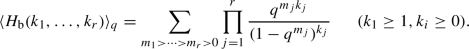
• (ii) The binomial model $\mathcal {F}=\textrm{b}$ corresponds to the so-called Schlesinger–Zudilin q-analogues of multiple zeta values [26, 33] given by

  

• (iii) Shifted binomial polynomials correspond to the q-analogues of multiple zeta values introduced by Bradley [11] and Zhao given by

  

The three products on the space of all functions on partitions naturally reduce to $\mathbb {P}$. That is, we obtain three commutative $\mathbb {Q}$-algebras $()$, and $(\mathbb {P}, \odot )$ with a natural involution, as stated in the following result.

Proposition 3.11

The space $\mathbb {P}$ of polynomial function on partitions

• (i) is closed under the conjugation $\iota$.

• (ii) is closed under the harmonic, shuffle and pointwise products , and $\odot$.

• (iii) has D (see Definition 2.3) as a derivation on both and .

• (iv) admits the algebra homomorphisms given in the following commutative diagram of differential $\mathbb {Q}$-algebras (with the derivation $q\frac{d}{dq}$ on $\mathcal {Z}_q$)

  

Proof

The first statement follows since the conjugate of $(r_1,\ldots , r_d)\times (m_1,\ldots , m_d)$ is given by $(m_1, m_{2}-m_1,\ldots ,m_d-m_{d-1})\times (r_1+\ldots +r_d,\ldots ,r_1)$ and therefore the conjugate of a polynomial in Stanley coordinates is again a polynomial in Stanley coordinates. Statement (ii) follows from Proposition 3.9 together with Corollary 3.8, since the harmonic, as well as the pointwise product, of two $\underline{u}$-brackets of can again be expressed as a linear combination of $\underline{u}$-brackets of . We will see this explicitly in Proposition 4.13. Together with (i) this then also shows that the space is closed under . Since D is the derivation on $\mathbb {Q}\llbracket u_1,u_2,\ldots \rrbracket$, defined on the generators by $D u_n =n u_n\,$, (iii) follows immediately by the fact that both  and  are defined via the $\underline{u}$-bracket. Finally (iv) follows from (i)–(iii) and the definition of  by the $\underline{u}$-bracket after setting $u_n = q^n$. $\square$

Remark 3.12

The space $\mathbb {M}\subset \mathbb {P}$ is also closed under $\iota$ and the products , . Moreover, since the space of quasimodular forms is closed under $q \frac{d}{dq}$, the space $\mathbb {M}$ is closed under D as well, i.e., $\mathbb {M}$ satisfies almost all properties of Proposition 3.11. But one can check that $\mathbb {M}$ is not closed under $\odot$. In general, it is not clear how $\mathbb {M}$ can be described explicitly as a subspace of $\mathbb {P}$. Since it contains the kernel of the q-bracket, it might be difficult to give an explicit description. In this note, we will give several examples of explicit elements in $\mathbb {M}$, but expect that there are many more (see, e.g., Example 5.2). Another open question is if there are other interesting subalgebras of $\mathbb {P}$, which satisfy (some of) the properties of Proposition 3.11.

Remark 3.13

The space $\mathbb {P}$ is not closed under the conjugation $\omega$. For example, for $\mathcal {F}$ well-normalized equals the biggest part of the partition $\lambda$. It is a small computation to verify that

$$\begin{aligned} \langle \lambda _1 \rangle _{\underline{u}} = - \sum _{\lambda \in \mathscr {P}} \mu (\lambda )\, \lambda _\ell \, u_{\lambda } \,\not \in \,\langle \mathbb {P}\rangle _{\underline{u}}\qquad (\ell =\ell (\lambda ) \text { is the } length~\text {of } \lambda ). \end{aligned}$$

The subspace $\Lambda ^*$ of $\mathbb {P}$, defined in the introduction, however, has the remarkable property that it is closed under $\omega$ but not under $\iota$.

Remark 3.14

For the Bernoulli–Seki model $\mathcal {F}=\textrm{s}$ the involution $\iota$ is explicitly given by

(3.6)

where for $\underline{a},\underline{b},\underline{d},\underline{k}\in \mathbb {Z}^r$ the constant $C^{\underline{a},\underline{k}}_{\underline{b},\underline{d}}$ is given by

$$\begin{aligned} C^{\underline{a},\underline{k}}_{\underline{b},\underline{d}} = (-1)^{|\underline{b}|}\prod _{j=1}^r\textstyle \left( {\begin{array}{c}s_j(\underline{d})-s^j(\underline{a})+j-1\\ a_{r-j+1}-1\end{array}}\right) \left( {\begin{array}{c}k_{r-j+1}-1\\ s_j(\underline{b})-s^j(\underline{k})+j-1\end{array}}\right) \frac{(a_j-1)!}{(k_j-1)!}(-1)^{s_j(\underline{k})+s^j(\underline{b})+j} \end{aligned}$$

and where for $\underline{\ell }\in \mathbb {Z}^r$ and $j=1,\ldots ,r$, we write

$$\begin{aligned} s_j(\underline{\ell }) = \sum _{i=1}^j \ell _i, \qquad s^j(\underline{\ell }) = \sum _{i=r-j+2}^r \ell _i. \end{aligned}$$

Since the q-bracket is $\iota$-invariant, (3.6) gives explicit linear relations among the q-brackets of the Bernoulli–Seki model (3.4). This corresponds to the partition relation in [2, Theorem 2.3]. There it was also conjectured that these families of relations together with the stuffle product are enough to write any q-series (3.4) as a linear combination of those with either $d_1=\dots =d_r=0$ or $k_1=\dots =k_r=1$. In our setup here this translates to the following model independent conjecture:

Conjecture 3.15

We have

$$\begin{aligned} \mathcal {Z}_q = \langle \mathbb {P}\rangle _q = \langle \mathbb {P}\cap \mathscr {H}\rangle _q = \langle \mathbb {P}\cap \!\mathscr {J}\rangle _q\,. \end{aligned}$$

Notice that the first equation here is known as explained in the remark at the beginning of Sect. 3.3 and the last equation is clear since $\iota (\mathbb {P}\cap \mathscr {H}) = \mathbb {P}\cap \mathscr {J}$. The functions in $\mathbb {P}\cap \mathscr {H}$ are exactly those polynomial functions on partitions where the polynomials in Definition 1.1 are independent of the variables $x_i$. This conjecture was also discussed in more detail for the Bernoulli–Seki model in [6] and [13].

3.4 Some remarks about the Möller transform

In contrast to the conjugation, products and derivation above, some natural operations on functions on partitions do not leave the space of polynomial functions invariant. One of the most interesting such operators is the Möller transform $\mathcal {M}:\mathbb {Q}^\mathscr {P}\rightarrow \mathbb {Q}^\mathscr {P}$ in [14]:

Definition 3.16

Given $f:\mathscr {P}\rightarrow \mathbb {Q}$, its Möller transform $\mathcal {M}f:\mathscr {P}\rightarrow \mathbb {Q}$ is the function given on a partition $\lambda$ of size n by

$$\begin{aligned} \mathcal {M}f(\lambda ) = \frac{1}{n!} \sum _{\mu \in \mathscr {P}(n)} |C_\mu |\,\chi _\lambda (\mu )^2 \, f(\mu ), \end{aligned}$$

where $|C_\mu |$ denotes the size of the conjugacy class associated to $\mu$ in the symmetric group $\mathfrak {S}_n\,$, and $\chi _\lambda (\mu )$ denotes value of the character of the irreducible representation of $\mathfrak {S}_n$ associated to $\lambda$ at any element in the conjugacy class associated to $\mu$.

The key property of the Möller transform (which follows directly from the second orthogonality relation for the characters of the symmetric group) is that for all $f:\mathscr {P}\rightarrow \mathbb {Q}$ one has

$$\begin{aligned} \langle \mathcal {M}f\rangle _q = \langle f \rangle _q. \end{aligned}$$

For the following subvectorspace of $\mathbb {P}$, the Möller transform is known to preserve the space of polynomial functions:

Proposition 3.17

Let $f\in \mathbb {P}$. Then $\mathcal {M}(f)\in \mathbb {P}$ if f is in the vector space generated by the constant function 1 and

for any $k\ge 2$ and $m\ge 0$.

Remark 3.18

As the statement of this proposition does not depend on the choice of $\mathcal {F}$, we also omit it from the notation.

Proof

For all $k\ge 1$, the Möller transform equals the hook-length moment $T_k\,$, given by

$$\begin{aligned} T_k(\lambda ):=\sum _{\xi \in Y_\lambda } h(\xi )^{k-2}, \end{aligned}$$

where $Y_\lambda$ denotes the Young diagram of $\lambda$, $\xi$ a cell in this diagram and $h(\xi )$ the hook-length of this cell. Note that for even k this function lies in the space of shifted symmetric functions defined in the introduction, as is shown in [14, Thm. 13.5]. For all $k\ge 2$, the results of Sect. 5.3 imply that is a polynomial function on partitions.

Also, any polynomial in $|\lambda |$, that is, any polynomial in with respect to $\odot$ is invariant under the Möller transform—as follows easily from the first orthogonality relation. In fact, from which the result follows. $\square$

Remark 3.19

For , the situation is totally different. In this case

As the q-bracket of a function and its Möller transform agree, we would expect this function to be of weight 1 as well, if it were a polynomial function on partitions. It is a matter of linear algebra to check that is not a polynomial function on partitions of weight $\le 1$.

In fact, the 233-dimensional vector space of polynomial functions on partitions of weight $\le 6$ only has a 10-dimensional subspace for which the Möller transform is again a polynomial function on partitions—this subspace is generated by 1, for $k=2,\ldots ,6$, and .

Lemma 3.20

For $f\in \mathbb {P}_{\le 6}$ the converse in Proposition 3.17 holds.

Note that this lemma can be proven by finding the kernel of a matrix containing at least $2\cdot 233+1$ values of all these polynomial functions as well as of their Möller transforms, as we did in Pari/GP. Hence, it seems the converse of Proposition 3.17 holds for all $f\in \mathbb {P}$.

4 From partitions to multiple zeta values

4.1 Weight and degree limits of partition analogues

For functions ${f\in \mathbb {P}}$, recall ${{\,\mathrm{Z^{{{\,\textrm{deg}\,}}}}\,}}(f)$ and $\textrm{deg}(f)$ are defined such that

$$\begin{aligned} (1-q)^{\textrm{deg}(f)}\langle f \rangle _q = {{\,\mathrm{Z^{{{\,\textrm{deg}\,}}}}\,}}(f) + O(1-q) \end{aligned}$$

asymptotically for real q. We will see that the degree is a non-negative integer bounded above by the weight of f. In this section, we prove Theorem 1.2. That is, we compute this degree and show that ${{\,\mathrm{Z^{{{\,\textrm{deg}\,}}}}\,}}(f)$ is a multiple zeta value, which justifies calling the elements of $\mathbb {P}$ partition analogues of multiple zeta values. From now on, we omit the well-normalized family $\mathcal {F}$ from the notation and write P instead of $P_\mathcal {F}$, unless the results depend on the choice of $\mathcal {F}$.

To get started we discuss two examples. First of all, we consider the degree of derivatives of polynomial functions on partitions.

Lemma 4.1

Given $f\in \mathbb {P}$, we have

$$\begin{aligned} \deg (Df) = \deg f +1, \qquad {{\,\mathrm{Z^{{{\,\textrm{deg}\,}}}}\,}}(Df) = \deg f \cdot {{\,\mathrm{Z^{{{\,\textrm{deg}\,}}}}\,}}(f). \end{aligned}$$

Proof

This follows directly from L’Hôpital’s rule, as for all $k\ne 0$ one has

$$\begin{aligned} \lim _{q\rightarrow 1} (1-q)^k \langle f\rangle _q&= \lim _{q\rightarrow 1} \frac{1}{k} (1-q)^{k+1} q\frac{\partial }{\partial q}\langle f\rangle _q = \lim _{q\rightarrow 1} \frac{1}{k} (1-q)^{k+1} \langle Df\rangle _q\,. \end{aligned}$$

$\square$

As another example, we consider polynomial functions on partitions of depth $\le 1$, corresponding to single zeta values. To calculate degree limits explicitly we define for $k\ge 1$ the (slightly modified) Eulerian polynomials $E_k$ by

$$\begin{aligned} \frac{E_k(X)}{(1-X)^k} :=\sum _{d\ge 1} \frac{d^{k-1}}{(k-1)!} X^d . \end{aligned}$$

(4.1)

Also, write $[n]_q=\frac{1-q^n}{1-q} = 1+q+\dots +q^{n-1}$.

Lemma 4.2

Let $k\ge 1, d\ge 0$. Then,

Proof

Consider the limit $q\rightarrow 1$ of the function $(1-q)^a \sum _{m,n} \frac{m^{k-1}}{(k-1)!}n^{d} q^{mn}$, which is the only term contributing to the degree limit for any well-normalized family. For $a=k$, this equals

$$\begin{aligned} \sum _{n\ge 1} n^d \,\frac{E_{k}(q^n)}{[n]_q^k}. \end{aligned}$$

(4.2)

By Proposition 4.5 below the terms in the sum (4.2) are bounded by $(k+1)n^{d-k}$ and therefore the sum converges absolutely if $k-d>1$. As $\lim _{q\rightarrow 1} \frac{E_k(q^n)}{[n]_q^k} = \frac{1}{n^k}$, in that case it follows that

Conversely, one obtains the case $k-d<1$ by the same argument interchanging the roles of k and d. Finally, in case $k-d=1$, a more careful analysis as in [25], shows the limit diverges—in accordance with the divergence of $\zeta (1)$. Also, after letting $a=k+\epsilon$ and $k-\epsilon$ for some $\epsilon >0$, the limit converges to 0 and diverges to $+\infty$ respectively. $\square$

Remark 4.3

Note that Lemma 4.1 and Lemma 4.2 are in agreement with the relation .

In the previous lemma, the proof of absolute convergence of the sum (4.2) was postponed. Note that by applying the techniques for asymptotics of sums of the form $\sum _{n} f(nt)$ in [31], as was previously observed in [34, Lemma 1], one obtains the following lemma (where the Eulerian polynomials $E_k$ are defined by (4.1)).

Lemma 4.4

For $k,n\ge 1$

$$\begin{aligned} \frac{E_k(q^n)}{[n]^k_q} = \frac{1}{n^k} + O(1-q), \qquad (q\rightarrow 1^{-}). \end{aligned}$$

We will give an upper bound for the left-hand side for all $q\in [0,1]$ in the following proposition. The special cases $k=1,2$ were obtained before in [5, Lemma 6.6(ii)].

Proposition 4.5

For $k,n\ge 1$ and $q\in [0,1]$ we have

$$\begin{aligned} \frac{E_{k}(q^{n})}{[n]_{q}^{k}} \,\le \, \frac{k+1}{n^{k}}. \end{aligned}$$

Proof

By continuity, we may assume $q\in (0,1)$. By definition, we have

$$\begin{aligned} \frac{E_{k}(q^{n})}{[n]_{q}^{k}} = \frac{E_{k}(q^{n})}{(1-q^{n})^{k}}\,(1-q)^{k} = \biggl (\sum _{d\ge 1}\frac{d^{k-1}}{(k-1)!}q^{dn}\biggr )(1-q)^{k}. \end{aligned}$$

Thus, it suffices to show

$$\begin{aligned} \biggl (\sum _{d\ge 1}\frac{d^{k-1}}{(k-1)!}q^{dn}\biggr )\,(1-q)^{k} \,\le \, \frac{k+1}{n^{k}} \qquad (k,n\ge 1, q\in (0,1)). \end{aligned}$$

We have

$$\begin{aligned} \sum _{d\ge 1}{d^{k-1}}\,q^{dn}&= \biggl (\log \frac{1}{q}\biggr )\, \sum _{d\ge 1}{d^{k-1}}\int _{dn}^{\infty }q^{u}\,du\\&= \biggl (\log \frac{1}{q}\biggr )\, \int _{n}^{\infty } \biggl (\sum _{1\le d\le u/n}{d^{k-1}}\biggr )\, q^{u}\,du, \end{aligned}$$

where interchanging the sum and integral is allowed since the sum $\sum _{d\ge 1}{d^{k-1}}q^{dn}$ converges (absolutely) for $q\in (0,1)$. For $u\ge n$, we now have

$$\begin{aligned} \sum _{1\le d\le u/n}{d^{k-1}} \,&= \sum _{1\le d\le \lfloor u/n\rfloor -1}\!\!{d^{k-1}} + \biggl (\frac{u}{n}\biggr )^{k-1}\\&\le \sum _{1\le d\le \lfloor u/n\rfloor -1}\int _{d}^{d+1}{y^{k-1}}\,dy + \biggl (\frac{u}{n}\biggr )^{k-1}\\&\le \, \int _{1}^{u/n}{y^{k-1}}\,dy + \biggl (\frac{u}{n}\biggr )^{k-1}\\&\le \, \frac{k+1}{k}\biggl (\frac{u}{n}\biggr )^{k}. \end{aligned}$$

We thus have

$$\begin{aligned} \begin{aligned} \sum _{d\ge 1}\frac{d^{k-1}}{(k-1)!}q^{dn} \,&\le \, \frac{k+1}{k!}\frac{1}{n^{k}} \biggl (\log \frac{1}{q}\biggr ) \int _{n}^{\infty } q^{u}\,u^{k}\,du\\&=\, \frac{k+1}{k!}\frac{1}{n^{k}} \biggl (\log \frac{1}{q}\biggr )^{-k} \int _{n\log \frac{1}{q}}^{\infty } e^{-u}\,u^{k}\,du\\&\le \, \frac{k+1}{k!}\frac{1}{n^{k}} \biggl (\log \frac{1}{q}\biggr )^{-k} \int _{0}^{\infty } e^{-u}\,u^{k}\,du\\&=\, \frac{k+1}{n^{k}} \biggl (\log \frac{1}{q}\biggr )^{-k}. \end{aligned} \end{aligned}$$

By using the bound

$$\begin{aligned}\log \frac{1}{q} = \int _{q}^{1}\frac{du}{u} \,\ge \, 1-q, \end{aligned}$$

we get

$$\begin{aligned} \biggl (\sum _{d\ge 1}\frac{d^{k-1}}{(k-1)!}q^{dn}\biggr )(1-q)^{k} \,\le \, \frac{k+1}{n^{k}}\, \biggl (\frac{1-q}{\log \frac{1}{q}}\biggr )^{k} \,\le \, \frac{k+1}{n^{k}}. \end{aligned}$$

$\square$

Remark 4.6

The stronger bound

$$\begin{aligned} \frac{E_{k}(q^{n})}{[n]_{q}^{k}} \,\le \, \frac{1}{n^{k}} \end{aligned}$$

(4.3)

fails for k divisible by 4, large n and q close to 1. Namely, setting $e^{-t}=q^n$, one finds that this inequality is equivalent to

$$\begin{aligned} \sum _{d\ge 1} \frac{d^{k-1}}{(k-1)!}\,e^{-dt}\,<\,\frac{1}{(n(1-e^{-t/n}))^k}. \end{aligned}$$

Note, $(n(1-e^{-t/n}))$ is bounded from below by t and converges to t as $n\rightarrow \infty$. As $t\downarrow 0$, one would deduce from this inequality that $\zeta (1-k) \,<\, 0$, which fails if $4\mid k$. Concretely, $k=4, q=e^{-10^{-4}}$ and $n=10^4$ provides a counterexample to (4.3).

To determine the degree of a polynomial function on partitions, we start with two estimates on this degree. Together, these statements are an improvement of the statement that the degree is bounded by the weight. In fact, in most cases, the degree is strictly smaller than the weight, so that the weight limit, defined below, vanishes in most cases.

Definition 4.7

For $f\in \mathbb {P}$ of weight $\le k$ which is not of weight $\le k-1$, the weight limit Z(f) is given by

$$\begin{aligned} Z(f) :=\lim _{q\rightarrow 1}(1-q)^{k}\langle f \rangle _q. \end{aligned}$$

Notice that Z is not a linear map.

Lemma 4.8

For all $\underline{k}$ and $\underline{d}$ one has

• (i)
• (ii)

Moreover, if there is no index t such that $k_i=1$ for all $i\le t$ and $d_i=0$ for all $i>t$, one has

Proof

Given $F\in \mathbb {Q}\llbracket q\rrbracket$, write $[q^n] F$ for the coefficient of $q^n$ in F. Forgetting the inequalities $m_1>m_2>\ldots >m_r\,$, one obtains

for all $n\in \mathbb {N}$, from which the first part of the statement follows using Lemma 4.2. The second statement follows by estimating $m_{i+1}^{d_{i+1}+1}\le m_{i+1}^{d_{i+1}}m_{i}\,$. Finally, if such a t does not exist, then the first two properties imply that the degree of the function at hand is strictly less than the weight, so that the weight limit vanishes. $\square$

We now prove Theorem 1.2, which determines the degree of a polynomial function

That is,

$$\begin{aligned} \textrm{deg}(f) = \max _{j\in \{0,\ldots ,r\}}\biggl \{\sum _{i\le j}(d_i+1) + \sum _{i> j}k_i\biggr \}. \end{aligned}$$

(4.4)

Recall that if $r=1$, by Lemma 4.2 the degree limit diverges if $k_1=d_1+1$. In general, this is the case when $k_a+\ldots +k_b = (d_a+1)+\ldots +(d_b+1)$ for some indices $a\le b$. If such indices do not exist, the maximum in (4.4) is unique and we show the corresponding degree limit is a sum of multiple zeta values. For this, we first show that multiple zeta values are also well-defined for certain indices with negative integers (cf., [22, Theorem 3]).

Lemma 4.9

For $r\ge 1$ and $\kappa _1,\ldots ,\kappa _r \in \mathbb {Z}$ with $\sum _{i=1}^j \kappa _i>j$ for all $j\ge 1$,

$$\begin{aligned} \zeta (\kappa _1,\ldots ,\kappa _r) :=\sum _{m_1>\cdots>m_r>0 }\frac{1}{m_1^{\kappa _1}\cdots m_r^{\kappa _r}} \end{aligned}$$

is a well-defined real number. Moreover, it is an element of $\mathcal {Z}_{\le |\kappa |}$.

Proof

First, we estimate $m_r^{-\kappa _r}$ by $m_{r-1}^{-\kappa _r+1}m_r^{-1}$ if $\kappa _r\le 0$ and obtain

$$\begin{aligned} 0\,<\,\zeta (\kappa _1,\ldots ,\kappa _r) \,\le \, \zeta (\kappa _1,\kappa _2,\ldots ,\kappa _{r-1}+\kappa _r-1,1) \end{aligned}$$

if $\kappa _r\le 0$. Iteratively (at most $r-1$ times) performing this procedure by estimating $m_i^{-\kappa _i'}$ by $m_{i-1}^{-\kappa _i'+1}m_i^{-1}$ for the largest index i for which the exponent $\kappa _i'$ of $m_i$ is non-positive, we find

$$\begin{aligned} 0<\zeta (\kappa _1,\ldots ,\kappa _r)\, \le \,\zeta (\kappa _1+\kappa _2+\ldots +\kappa _j-j+1,\ldots ) \, <\,\infty \end{aligned}$$

for some $j\ge 1$, where by the nature of this iterative process only the first entry may be non-positive. By our assumption $\sum _{i=1}^j \kappa _i>j$, we find that the first entry is at least equal to 2, from which we indeed conclude that $\zeta (\kappa _1,\ldots ,\kappa _r)$ is a well-defined real number.

By iteratively using that $\sum _{m=a}^b m^{-k}$ for $k\le 0$ is a polynomial in a and b, it is not hard to show that $\zeta (\kappa _1,\ldots ,\kappa _r)\in \mathcal {Z}_{\le |\underline{\kappa }|},$ with $|\underline{\kappa }|=\sum _{i}\kappa _i\,$. Observe, here, again we make use of the assumption $\sum _{i=1}^j \kappa _j>j$ to ensure all multiple zeta values in this linear combination are convergent. $\square$

Proof of Theorem 1.2

Let $j=t$ be the smallest index for which the maximum in (4.4) is attained. Write and We will show that ${{\,\mathrm{Z^{{{\,\textrm{deg}\,}}}}\,}}g$ and ${{\,\mathrm{Z^{{{\,\textrm{deg}\,}}}}\,}}h$ are multiple zeta values in case $j=t$ is the unique index for which the maximum in (4.4) is attained. In that case, we also show that ${{\,\mathrm{Z^{{{\,\textrm{deg}\,}}}}\,}}f = ({{\,\mathrm{Z^{{{\,\textrm{deg}\,}}}}\,}}g )( {{\,\mathrm{Z^{{{\,\textrm{deg}\,}}}}\,}}h).$

Since the degree limit only depends on the leading term we can choose any well-normalized family $\mathcal {F}$. Observe that if we choose the Bernoulli–Seki model we have

$$\begin{aligned} \langle h\rangle _q&= \sum _{m_{t+1}>\ldots>m_r>0} \prod _{i} m_i^{d_i} \frac{E_{k_i}(q^{m_i})}{(1-q^{m_i})^{k_i}}. \end{aligned}$$

(4.5)

By Lemma 4.4 we get for all i

$$\begin{aligned} \lim _{q\rightarrow 1} m_i^{d_i} (1-q)^{k_i}\frac{E_{k_i}(q^{m_i})}{(1-q^{m_i})^{k_i}} = m_i^{d_i-k_i}. \end{aligned}$$

First, assume $j=t$ is the unique index for which the maximum in (4.4) is attained. Then, we know that for all $t'> t$

$$\begin{aligned} \sum _{i=t+1}^{t'} k_i >\sum _{i=t+1}^{t'} (d_i+1). \end{aligned}$$

(4.6)

By Proposition 4.5 we find that the sum in (4.5) is absolutely bounded by a constant (depending on the $k_i$) times $\zeta (k_{t+1}-d_{t+1},\ldots ,k_r-d_r)$. Using (4.6), this multiple zeta value is well-defined by Lemma 4.9, so (4.5) converges absolutely. By interchanging the sum and limit, we conclude

$$\begin{aligned} {{\,\textrm{deg}\,}}h = \sum _{i=t+1}^r k_i \quad \text {and} \quad {{\,\mathrm{Z^{{{\,\textrm{deg}\,}}}}\,}}h = \zeta (k_{t+1}-d_{t+1},\ldots ,k_r-d_r). \end{aligned}$$

Hence, ${{\,\mathrm{Z^{{{\,\textrm{deg}\,}}}}\,}}h$ is a linear combination of multiple zeta values of weight $\le \sum _{i=t+1}^r k_i\,$.

In case the index $j=t$ is not unique, let $\epsilon >0$. Then, as

$$\begin{aligned} \lim _{q\rightarrow 1} m_i^{d_i} (1-q)^{k_i+\epsilon } \frac{E_{k_i}(q^{m_i})}{(1-q^{m_i})^{k_i}} \,\rightarrow \, 0 \end{aligned}$$

if $q\rightarrow 1$, we see that $\deg h \le \sum _{i=t+1}^r k_i$ in this case. Moreover, as

$$\begin{aligned} \lim _{q\rightarrow 1} m_i^{d_i} (1-q)^{k_i} \frac{E_{k_i}(q^{m_i})}{(1-q^{m_i})^{k_i}} = m_i^{d_i-k_i} \,>\,0, \end{aligned}$$

we conclude that also in this case we have $\deg h = \sum _{i=t+1}^r k_i$.

Next, (again working with the Bernoulli–Seki model) observe that

$$\begin{aligned} \langle g \rangle _q&= \sum _{\begin{array}{c} m_{1}>\ldots>m_t>0 \\ r_{1},\ldots ,r_t>0 \end{array}} \prod _{i} m_i^{d_i}r_i^{k_i-1} q^{m_i r_i} \\&= \sum _{\begin{array}{c} 0<r_{1}'<\ldots <r_t' \\ m_{1}',\ldots ,m_t'>0 \end{array}} \prod _{i} (m_i'+\ldots +m_t')^{d_i} (r_i'-r_{i-1}')^{k_i-1} q^{m_i' r_i'}, \end{aligned}$$

where we set $r_0'=0$. Given a ‘monomial’ $m_1^{d_1'}\cdots m_t^{d_t'}$, we have

$$\begin{aligned} \sum _{\begin{array}{c} 0<r_{1}<\ldots<r_t \\ m_{1},\ldots ,m_t>0 \end{array}} \prod _{i} m_i^{d_i'} q^{m_i r_i}&= \sum _{0<r_{1}<\ldots <r_t} \prod _{i} d_i'! \frac{E_{d_i'+1}(q^{r_i})}{(1-q^{r_i})^{d_i'+1}}, \end{aligned}$$

which is of degree $\sum _{i} (d_i'+1)$ and (in case $d_t'>0$) with degree limit $\zeta (d_t'+1,\ldots ,d_1'+1)$ (as follows from above). Hence, by expanding $\prod _{i}(m_i'+\ldots +m_t')^{d_i}$ in monomials, we see that

$$\begin{aligned} {{\,\textrm{deg}\,}}g = \sum _{i}(d_i+1), \end{aligned}$$

provided that the corresponding limit

$$\begin{aligned} L = \sum _{0<r_1<\ldots <r_t} \prod _i \frac{(r_i-r_{i-1})^{k_i-1}}{r_i}\cdot \Omega \biggl [\prod _{i=1}^t \Bigl (\frac{1}{r_i}+\ldots +\frac{1}{r_t}\Bigr )^{d_i}\biggr ], \end{aligned}$$

converges, where $\Omega :\mathbb {Q}[r_1^{-1},\ldots ,r_t^{-1}]\rightarrow \mathbb {Q}[r_1^{-1},\ldots ,r_t^{-1}]$ is the linear mapping (1.7), i.e.,

$$\begin{aligned} \Omega \Bigl [\frac{1}{r_1^{l_1}\cdots r_t^{l_t}}\Bigr ] :=\frac{l_1!\cdots l_r!}{r_1^{l_1}\cdots r_t^{l_t}} \qquad \qquad (l_i\in \mathbb {Z}_{\ge 0}). \end{aligned}$$

Note that $\langle g\rangle _q$ is bounded by a constant (only depending on the $d_i'$) times L, which justifies interchanging the sum and limit in this computation (if L converges). We estimate

$$\begin{aligned} r_i-r_{i-1}\le r_i \qquad \text {and} \qquad \frac{1}{r_i}+\ldots +\frac{1}{r_t}\le \frac{t}{r_i} \end{aligned}$$

to obtain

$$\begin{aligned} L \,\le \, \sum _{0<r_1<\ldots <r_t} \prod _i r_i^{k_i-d_i} t^{d_i} d_i! = \biggl (\prod _{i} t^{d_i}d_i!\biggr )\cdot \zeta (d_t-k_t,\ldots ,d_1-k_1). \end{aligned}$$

Note that if for some s we have that $\sum _{i=s}^t (d_i-k_i+1)\le 0$, then the sum (4.4) is also maximized for $j=s-1$, contradicting the definition of t. Hence, Lemma 4.9 implies that L is a well-defined real number. Therefore, $L={{\,\mathrm{Z^{{{\,\textrm{deg}\,}}}}\,}}g$ and ${{\,\mathrm{Z^{{{\,\textrm{deg}\,}}}}\,}}g$ is a well-defined linear combination of multiple zeta values of weight $\le \sum _{i=1}^t (d_i+1)$ (the latter one reads of from the definition of L).

Finally, we relate the degree and limits of g and h to the degree and limits of f. Consider the difference , and observe that (as ; see Proposition 2.5). First, we assume again that $j=t$ is the unique index for which the maximum in (4.4) is attained. In that case, we claim that is of smaller degree than . It follows from this claim that the function f has the same degree, as well as degree limit, as . Hence, in case $j=t$ is the unique index for which the maximum in (4.4) is attained, it suffices to prove the claim.

To prove the claim, we write this difference in terms of the basis elements of $\mathbb {P}$. Then, we will see it contains two types of terms. We show that all these terms are of degree smaller than the degree (4.4) in the statement.

First of all, there are terms in where the column with $k_t$ and $d_t$ is on the right of the column with $k_{t+1}$ and $d_{t+1}$ (note that possibly some other column is stuffled on the columns containing these values). We apply Lemma 4.8(ii) repeatedly, so that:

• The values $d_j$ are replaced by $d_j'$ such that $k_j\le d_{j}'+1$ if $j\le t$ and $k_t< d_{t}'+1$, and with $k_j\ge d_{j}'+1$ if $j>t$ and $k_{t+1}>d_{t+1}'+1$. That this is always possible follows from the construction of t. For the strict inequalities, we use the uniqueness of the maximum defining t.

• Additionally, the values $d_t'$ and $d_{t+1}'$ are replaced by $d_t'-1$ and $d_{t+1}'+1$ respectively.

Lemma 4.8(i) now implies that these terms are of lower degree.

Secondly, there are terms of depth $<r$, for which a certain column is given by $\left( {\begin{array}{c}k_t+k_{t+1}-a\\ d_t+d_{t+1}\end{array}}\right)$ for some $a\ge 0$. Then, similarly, Lemma 4.8 also implies that these terms are of lower degree.

Now, the case that $j=t$ is not the unique index for which the maximum in (4.4) is attained remains. By a similar argument as in Lemma 4.8(i), we have

$$\begin{aligned} \deg f \le \deg g + \deg h. \end{aligned}$$

Namely, for this inequality, we forget all inequalities $m_i>m_j$ if $i\le t$ and $j>t$.

Let $j=t'$ be the maximal index for which the maximum in (4.4) is obtained, and write

Now, we apply Lemma 4.8(ii) for $i=1,\ldots ,t'-1$, to obtain a lower bound for the degree of f. That is,

Here, the last equality holds as for $f'$ the maximum in (4.4) is uniquely attained at $j=t'$, and we already computed the degree and corresponding limit in that case. Hence, $\deg f$ is bounded from both sides by the value (4.4), which completes the proof in the case that $j=t$ is not the unique index for which the maximum in (4.4) is attained. $\square$

Recall that by Lemma 4.8 we have

if there is no index t such that $k_i=1$ for all $i\le t$ and $d_i=0$ for all $i>t$. By going through the proof above for those basis elements in $\mathbb {P}$ for which there does exist such a t, we find that the weight limits of such elements do not vanish:

Corollary 4.10

For all $d_1,\ldots ,d_{t-1}\ge 0, d_t\ge 1, k_{t+1}\ge 2$ and $k_{t+2},\ldots ,k_{r}\ge 1$, write

We have

$$\begin{aligned} {{\,\textrm{deg}\,}}f = \sum _{i=1}^t (d_i+1) + \sum _{i=t+1}^r k_i = {{\,\textrm{wt}\,}}f \end{aligned}$$

and

$$\begin{aligned} {{\,\mathrm{Z^{{{\,\textrm{deg}\,}}}}\,}}f = \xi (d_1,\dots ,d_t) \, \zeta (k_{t+1}, \dots , k_r) = Z f. \end{aligned}$$

4.2 Algebraic setup

We will now introduce the algebraic setup for our space $\mathbb {P}$ by generalizing the classical setup introduced by Hoffman in [17] and used in [20] for the regularization of multiple zeta values. For each model $\mathcal {F}=\{f_k\}_{k=0}^\infty$ of well-normalized polynomials we will describe the harmonic product as well as the shuffle product on the level of words in analogy to [17]. For the Bernoulli–Seki model the algebraic setup described here coincides with the one described in [2, Section 3]. Define the set A, also called the set of letters, by

We will define a product $*_{\mathcal {F}}$ on the space $\mathbb {Q}\langle A \rangle$ of non-commuting polynomials in A and we will call a monic monomial in $\mathbb {Q}\langle A \rangle$ a word. This product on the space of words will depend on a product $\diamond _{\mathcal {F}}$ on the space $\mathbb {Q}A$ of letters, which depends on $\mathcal {F}$. Recall that as $\mathcal {F}$ is well-normalized, the $f_k$ are polynomials of degree k with leading coefficient $\frac{1}{k!}$. Then, for $k_1,k_2 \ge 1$ and $1 \le j \le k_1+k_2-1$ there exist rational numbers $\alpha _\mathcal {F}(k_1,k_2,j) \in \mathbb {Q}$ such that for all $n \ge 1$

$$\begin{aligned} \sum _{\begin{array}{c} n_1+n_2=n\\ n_1,n_2\ge 1 \end{array}} \partial f_{k_1}(n_1)\, \partial f_{k_2}(n_2) = \partial f_{k_1+k_2}(n) + \sum _{j=1}^{k_1+k_2-1} \alpha _\mathcal {F}(k_1,k_2,j)\, \partial f_{j}(n)\,, \end{aligned}$$

(4.7)

where as before $\partial f(n)=f(n)-f(n-1)$ for integers $n\ge 1$.

Example 4.11

• (i) If $\mathcal {F}=\textrm{b}$ is the binomial model, i.e., $f_k(x)=\left( {\begin{array}{c}x\\ k\end{array}}\right)$, we have $\partial f_k(x) = \left( {\begin{array}{c}x-1\\ k-1\end{array}}\right)$ for $k\ge 1$ and since

  $$\begin{aligned} \sum _{\begin{array}{c} n_1+n_2=n\\ n_1,n_2\ge 1 \end{array}} \left( {\begin{array}{c}n_1-1\\ k_1-1\end{array}}\right) \left( {\begin{array}{c}n_2-1\\ k_2-1\end{array}}\right) = \left( {\begin{array}{c}n-1\\ k_1+k_2-1\end{array}}\right) \end{aligned}$$

  we obtain $\alpha _\textrm{b}(k_1,k_2,j)=0$.

• (ii) For the Bernoulli–Seki model $\mathcal {F}=\textrm{s}$ we find that $\alpha _\textrm{s}(k_1,k_2,j)$ equals

  $$\begin{aligned} -\left( \!(-1)^{k_1} \left( {\begin{array}{c}k_1+k_2-1-j\\ k_2 -j\end{array}}\right) + (-1)^{k_2} \left( {\begin{array}{c}k_1+k_2-1-j\\ k_1-j\end{array}}\right) \!\right) \frac{B_{k_1+k_2-j}}{(k_1+k_2-j)!} \,, \end{aligned}$$

  (4.8)

  which can be proven by using Bernoulli’s/Seki’s/Faulhaber’s formula for the sum of powers (see, e.g., [28, Lemma 6.1.2(ii)]).

On $\mathbb {Q}A$ we define the product $\diamond _{\mathcal {F}}$ for $k_1, k_2 \ge 1$ and $d_1,d_2 \ge 0$ by

(4.9)

In the case $\mathcal {F}=\textrm{b}$ we just write $\diamond = \diamond _{\textrm{b}}\,$, which is given by

For each well-normalized family of polynomials $\mathcal {F}$ this gives a commutative non-unital $\mathbb {Q}$-algebra $(\mathbb {Q}A, \diamond _{\mathcal {F}})$. We will be interested in $\mathbb {Q}$-linear combinations of words in the letters of A and we define

$$\begin{aligned} \mathfrak {P}= \mathbb {Q}\langle A \rangle \end{aligned}$$

In the following we will use for $k_1,\dots ,k_r\ge 1$, $d_1,\dots ,d_r\ge 0$ the following notation to write words in $\mathfrak {P}$:

where the product on the right is the usual non-commutative product in $\mathbb {Q}\langle A \rangle$.

Definition 4.12

For a well-normalized family of polynomials $\mathcal {F}$ we define the quasi-shuffle product $*_{\mathcal {F}}$ on $\mathfrak {P}$ as the $\mathbb {Q}$-bilinear product, which satisfies $1 *_{\mathcal {F}}w = w *_{\mathcal {F}}1 = w$ for any word $w\in \mathfrak {P}$ and

$$\begin{aligned} a w *_{\mathcal {F}}b v = a (w *_{\mathcal {F}}b v) + b (a w *_{\mathcal {F}}v) + (a \diamond _{\mathcal {F}}b) (w *v) \end{aligned}$$

(4.10)

for any letters $a,b \in A$ and words $w, v \in \mathfrak {P}$.

We obtain a commutative $\mathbb {Q}$-algebras $(\mathfrak {P},*_{\mathcal {F}})$, as shown in [17] (see also [19]). In the case $\mathcal {F}=\textrm{b}$ we just write $*= *_{\textrm{b}}\,$. As an example for the product (4.10) we have

The algebra $(\mathfrak {P},*)$ is graded by weight, where the weight is defined by

and it is filtered by depth, which is defined by

In general the algebra $(\mathfrak {P},*_{\mathcal {F}})$ is not graded but filtered by weight.

Proposition 4.13

For any well-normalized family of polynomials $\mathcal {F}$ the maps

and

are algebra-isomorphisms of filtered algebras. Recall that $\textrm{m}$ stands for the monomial model (see Table 1).

Proof

Assume $\mathcal {F}$ is a well-normalized family of polynomials. First, notice that whenever one has a sum of the form

$$\begin{aligned} \sum _{m_1> \dots> m_r > 0} \prod _{j=1}^r m_j^{d_j}\, h(m_j,k_j) \end{aligned}$$

(4.11)

in a $\mathbb {Q}$-algebra $(A,\times )$ with some function h satisfying

$$\begin{aligned} h(m,k_1)\times h(m,k_2) = h(m,k_1+k_2) + \sum _{j=1}^{k_1+k_2-1} \alpha _\mathcal {F}(k_1,k_2,j)\, h(m,j)\,, \end{aligned}$$

(4.12)

then the linear map $\varphi$ defined by sending the generators to (4.11) satisfies $\varphi (w) \times \varphi (v)=\varphi (w *_{\mathcal {F}}v)$ for all $w,v\in \mathfrak {P}$. This can be shown by truncating the sum over the $m_j$ by some M and then doing induction on M together with the definition of $*_{\mathcal {F}}$ (see for example [3, Lemma 2.18]). To show the first statement we consider the $\underline{u}$-bracket of a generator of $\mathbb {P}$, which by Proposition 3.9 is given by

(4.13)

Since the harmonic product  is defined by the $\underline{u}$-bracket (see Definition 2.3) we see that $\Xi _\mathcal {F}$ is an algebra homomorphism, as (4.13) is a sum of the form (4.11) with $h(m,k) = \sum _{n>0} \partial f_{k}(n)\, u_{m}^{n}$ and the property (4.12) is satisfied due to (4.7). With a similar argument, we see that also the second map is an algebra homomorphism since

is a sum of the form (4.11) with $h(m,k)=r_{m}(\lambda )^{k}$. All maps are also isomorphisms among the elements in $\mathfrak {P}$ and in $\mathbb {P}$ (Corollary 3.8). $\square$

As a direct consequence of describing the product in terms of a quasi-shuffle product is the following.

Proposition 4.14

For $k\ge 2, d\ge 0$ with $k+d$ even we have , i.e., their q-brackets are quasimodular forms (of mixed weight).

Proof

Suppose a $\mathbb {Q}$-algebra R and an algebra homomorphism $\varphi : (\mathfrak {P},*_{\mathcal {F}}) \rightarrow R$ are given. Using [19, (32)] (see also [3, (2.13)]) we have for $a\in A$ the following equation in $R\llbracket X \rrbracket$:

$$\begin{aligned} \exp \left( \sum _{n=1}^{\infty } (-1)^{n-1} \varphi ( a^{\diamond _\mathcal {F}n}) \frac{X^n}{n} \right) = 1+ \sum _{n=1}^{\infty } \varphi (a^n) X^n, \end{aligned}$$

(4.14)

where $a^{\diamond _\mathcal {F}n} = \overbrace{a \diamond _\mathcal {F}\dots \diamond _\mathcal {F}a }^n \in \mathbb {Q}A$ and $a^n = \overbrace{a\cdots a}^n \in \mathfrak {P}$.

Now, let $R=\mathbb {Q}\llbracket q \rrbracket$ and let $\varphi$ be the composition of the algebra homomorphism $\Xi _\mathcal {F}$ in Proposition 4.13 with the q-bracket, so that we obtain an algebra homomorphism $\varphi : (\mathfrak {P},*_{\mathcal {F}}) \rightarrow \mathbb {Q}\llbracket q \rrbracket$ (see Proposition 3.11). We call a letter even if ${k\ge 2}$, ${d\ge 0}$ and $k+d$ is even. In the case $\mathcal {F}=\textrm{s}$ one then checks using (4.8) and (4.9) that for two even letters $a,a'\in A$, the product $a \diamond _\textrm{s} a'$ is again a linear combination of some even letters (the Bernoulli numbers $B_k$ for $k\ge 3$ odd vanish). This inductively gives that for an even letter a the element $a^{\diamond _\mathcal {F}n}$ is also a linear combination of even letters. Then (4.14) implies that the q-bracket of , which is $\varphi (a^n)$ for , can be written as a polynomial in the q-brackets of with $k'+d'$ even. By (3.5) for $\mathcal {F}=\textrm{s}$ these are exactly given by derivatives of Eisenstein series and therefore we obtain a quasimodular form (of mixed weight). $\square$

Example 4.15

For example, in the case $k=2$, $d=0$ we get in depth two

where we used .

The above algebraic setup can be seen as a generalization of the algebra $\mathfrak {H}^1$ defined in [17], as we explain now. Setting for $k\ge 1$ we define

$$\begin{aligned} \mathfrak {H}^1 = \mathbb {Q}+ \langle z_{k_1}\dots z_{k_r} \mid r\ge 1 , k_1,\dots ,k_r \ge 1\rangle _\mathbb {Q}\,\subset \, \mathfrak {P}\end{aligned}$$

and its subspace of admissible words

$$\begin{aligned} \mathfrak {H}^0 = \mathbb {Q}+ \langle z_{k_1}\dots z_{k_r} \in \mathfrak {H}^1 \mid r\ge 1 , k_1 \ge 2\rangle _\mathbb {Q}\,. \end{aligned}$$

The quasi-shuffle product on $\mathfrak {P}$ reduces to a product on $\mathfrak {H}^1$ and on $\mathfrak {H}^0$. Moreover, the product $*$ reduces to the classical harmonic product introduced in [17]. One can then define the following $\mathbb {Q}$-linear map²

$$\begin{aligned} \zeta : \mathfrak {H}^0&\longrightarrow \mathcal {Z}\nonumber \\ z_{k_1}\dots z_{k_r}&\longmapsto \zeta (k_1,\dots ,k_r)\,. \end{aligned}$$

(4.15)

By the definition of multiple zeta values (1.5) as nested sum one then checks that this map is an algebra homomorphism from $(\mathfrak {H}^0, *)$ to the algebra of multiple zeta values $\mathcal {Z}$. Since $\mathfrak {H}^1 = \mathfrak {H}^0[ z_1]$ ([20, Proposition 1]) one can extend this algebra homomorphism uniquely to an algebra homomorphism $\zeta ^*: (\mathfrak {H}^1, *) \rightarrow \mathcal {Z}[T]$ which satisfies $\zeta ^*(z_1)=T$ and $\zeta ^*_{\mid \mathfrak {H}^0} = \zeta$. This gives the definition of (harmonic) regularized multiple zeta values for $k_1,\dots ,k_r\ge 1$.

In the following we will generalize this result and the goal is to obtain an algebra homomorphism $(\mathfrak {P}, *) \rightarrow \mathcal {Z}[T]$. First, we define the analogue of admissible words in our larger space $\mathfrak {P}$.

Definition 4.16

• (i) For $d\ge 0$ set . As an counterpart of $\mathfrak {H}^1$ and $\mathfrak {H}^0$ we define

  $$\begin{aligned} \mathfrak {J}^1&= \mathbb {Q}+ \langle v_{d_1}\dots v_{d_r} \mid r\ge 1 , d_1,\dots ,d_r \ge 0\rangle _\mathbb {Q}\,\subset \, \mathfrak {P}\\ \mathfrak {J}^0&= \mathbb {Q}+ \langle v_{d_1}\dots v_{d_r} \in \mathfrak {J}^1 \mid r\ge 1 , d_r \ge 1\rangle _\mathbb {Q}\,. \end{aligned}$$

• (ii) We set $\mathfrak {P}^1:= \mathfrak {J}^1 \mathfrak {H}^1$, which is the space spanned by all words of the form

  

  (4.16)

  for some $j \ge 0$, $m,r \ge 0$, $d_m\ge 1$ (if $m\ge 1$), and $k_1\ge 2$ (if $r\ge 1$).

• (iii) A word $w\in \mathfrak {P}^1$ of the form (4.16) is called admissible if $j=0$. The subspace of admissible words will be denoted by

  $$\begin{aligned} \mathfrak {P}^0 :=\mathfrak {J}^0 \mathfrak {H}^0 = \langle w \in \mathfrak {P}^1 \mid w \text { is admissible} \rangle _\mathbb {Q}\,. \end{aligned}$$

Notice that this notion of admissibility coincides with the classical notion of admissibility on the subspace $\mathfrak {H}^1$, namely, we have $\mathfrak {H}^0 = \mathfrak {H}^1 \cap \mathfrak {P}^0$. However, in contrast to the classical setup, the spaces $\mathfrak {P}^1$ and $\mathfrak {P}^0$ are not closed under $*$ (or any $*_{\mathcal {F}}$) and therefore they are not subalgebras of $\mathfrak {P}$.

Lemma 4.17

Let $\mathfrak {N}$ be the subspace of $\mathfrak {P}$ spanned by all words in $\mathfrak {P}{\setminus } \mathfrak {P}^1$. Then $\mathfrak {N}$ is an ideal in $(\mathfrak {P}, *)$.

Proof

We need to show that for any $w \in \mathfrak {P}$ which is not of the form (4.16) the product $w *v$ is in $\mathfrak {N}$ for any $v \in \mathfrak {P}$. If $w \in \mathfrak {P}$ is not of the form (4.16) then w either contains a letter or it contains a letter  which is on the left of a letter  with $k\ge 2$ and $d\ge 1$ in both cases. In the first case, the product of w with any element v will be a sum of words which also contain either a letter  or a with some other letter b of v. Since $\diamond$ is the component-wise addition we see that each word therefore also contains a letter with top entry $\ge 2$ and bottom entry $\ge 1$. In the second case, all words either also have a letter  which is on the left of a letter , or a letter on the left of a letter , where b, c are letters of v, etc. In all cases, the words are not of the form (4.16) and are therefore elements in $\mathfrak {N}$. $\square$

As a generalization of $\mathfrak {H}^1 = \mathfrak {H}^0[ z_1]$, we will now show that any element in $\mathfrak {P}^1$ can be written as a polynomial with respect to the quasi-shuffle product $*$ with coefficients in $\mathfrak {P}^0$ up to elements in the ideal $\mathfrak {N}$. We write

Proposition 4.18

For any word $w \in \mathfrak {P}^1$ of length r there exist unique $w_j \in \mathfrak {P}^0$ such that

(4.17)

Moreover, if ${{\,\textrm{wt}\,}}(w)=k$ then the $w_j$ are linear combinations of words of weight $k-j$.

Proof

A word in $w\in \mathfrak {P}^1$ can be written as

Write and with $d_m>0$ and $k_1>1$. By definition of the quasi-shuffle product $*$ for $j\ge 1$ we have that equals

Here every displayed term, except for jw, is either an element in $\mathfrak {N}$ or is of the form , where $u'\in \mathfrak {J}^0$ and $v'\in \mathfrak {H}^0$ and $j'\le j-1$. By induction on j we therefore see that w can be written as in (4.17).

For the uniqueness assume that for some $w_j \in \mathfrak {P}^0$. Then the term is the only summand which contains classes of the form (4.16) with $j=r$. Since there are no relations among elements in $\mathfrak {P}^1$ modulo $\mathfrak {N}$ we immediately obtain $w_r = 0$ and therefore $w_j=0$ for all $j=1,\dots ,r$. $\square$

Example 4.19

For $k\ge 2,d\ge 1$ we have

Here $w_0,w_1 \in \mathfrak {P}^0$ and the last term is in $\mathfrak {N}$ due to the 2 in the top left entry.

We end this subsection by defining an analogue of the involution $\iota$ on the space $\mathfrak {P}$. Since Proposition 4.13 gives as for any well-normalized family of polynomials $\mathcal {F}$ an isomorphism we give the following definition.

Definition 4.20

For any well-normalized family of polynomials $\mathcal {F}$ we define the linear map $\iota _\mathcal {F}$ by

$$\begin{aligned} \iota _\mathcal {F}: \mathfrak {P}&\longrightarrow \mathfrak {P}\\ w&\longmapsto (\Xi _\mathcal {F}^{-1} \circ \iota \circ \Xi _\mathcal {F})(w)\,. \end{aligned}$$

When we choose the Bernoulli–Seki model $\mathcal {F}= \textrm{s}$, then the involution $\iota _\textrm{s}$ can be described nicely using generating series. That is, given a depth $r\ge 1$ we write $\mathfrak {A}$ for the formal power series in $\mathfrak {P}\llbracket X_1,Y_1,\dots ,X_r,Y_r\rrbracket$ given by

(4.18)

Proposition 4.21

We have

where the involution $\iota _\textrm{s}$ on the left is applied coefficient-wise.

Proof

This can be proven by using the same change of variables as it was done in [2, Theorem 2.3] by replacing the q-series there with the $\underline{u}$-bracket of $P_\textrm{s}$ and then using the explicit description of $\iota$ mentioned in the proof of Lemma 2.7. $\square$

4.3 Bi-multiple zeta values

We now combine the results of Sect. 4.1 and 4.2 to define a bi-variant of multiple zeta values. These can be seen as regularized limits of polynomial functions on partitions, since they are defined for arbitrary words $w \in \mathfrak {P}$.

Definition 4.22

We define the linear map

as follows:

• (i) For $w \in \mathfrak {N}$ we set $\zeta (w) = 0$.

• (ii) For $w\in \mathfrak {P}^0$ we write and set

  

  where $k_1\ge 2$, $d_m\ge 1$ and where $\xi$ is the conjugated multiple zeta value defined in Definition 1.3.

• (iii) For with $w_j \in \mathfrak {P}^0$ we set

  $$\begin{aligned} \zeta (w) = \sum _{j=0}^r \zeta (w_j) \,T^j\,. \end{aligned}$$

Notice that due to Proposition 4.18 and part (i) the value $\zeta (w)$ in (iii) is well-defined.

Theorem 4.23

For any well-normalized family of polynomials $\mathcal {F}$ the map

$$\begin{aligned} \zeta : (\mathfrak {P},*) \longrightarrow \mathcal {Z}[T] \end{aligned}$$

is an $\iota _\mathcal {F}$-invariant algebra homomorphism.

Proof

First, we show that $\zeta$ is an algebra homomorphism. Since $\mathfrak {N}$ is an ideal (Lemma 4.17) and $\zeta (w) = 0$ for $w \in \mathfrak {N}$, we can restrict to the case when $w \notin \mathfrak {N}$, i.e., $w \in \mathfrak {P}^1$. Moreover, we can restrict to the elements in $\mathfrak {P}^0$ due to the definition in (iii). If $w \in \mathfrak {P}^0$ we can assume that we can write with $d_m\ge 1$ (or $m=0$) and $k_1\ge 2$ (or $r=0$). Then we have by Corollary 4.10 that

(4.19)

where the weight limit Z is introduced in Definition 4.7. Now for $k\ge 1$ and $f \in \mathbb {P}$ set

$$\begin{aligned} Z_k(f) = \lim _{q\rightarrow 1}(1-q)^{k}\langle f \rangle _q\,, \end{aligned}$$

i.e., if k is the weight of f then $Z_k(f)$ is exactly the weight limit of f.

Let $w_1,w_2 \in \mathfrak {P}^0$ be given and write $k_1={{\,\textrm{wt}\,}}(w_1)$, $k_2= {{\,\textrm{wt}\,}}(w_2)$ and $k=k_1+k_2$. Then, we have by Proposition 4.13 that and . Comparing the definition of $*=*_\textrm{b}$ and $*_\textrm{s}\,$, we see that they are the same up to lower weight terms. In particular, their image under $Z_k$ is the same. Moreover, since $Z_k$ is defined via the q-bracket, which is an algebra homomorphism with respect to (Proposition 3.11), we get

But this also equals $\zeta (w_1 *w_2)$, since $w_1 *w_2$ is a linear combination of words which are either in $\mathfrak {P}^0$ (i.e., they can be written as in (4.19)) or which are in $\mathfrak {N}$. For the latter, the weight limit, and therefore the image under $Z_k\,$, vanishes as seen in Lemma 4.8.

It remains to show that $\zeta$ is $\iota _\mathcal {F}$-invariant for any well-normalized family of polynomials $\mathcal {F}$. Let with $w_j \in \mathfrak {P}^0$ and define the $\tilde{w}_j \in \mathfrak {P}^0$ by . We need to show that $\zeta (w_j) = \zeta (\tilde{w}_j)$ for all $j=0,\dots ,r$. Since the q-bracket is $\iota$ invariant we have $\langle \Xi _\mathcal {F}(w) \rangle _q = \langle \Xi _\mathcal {F}( \iota _\mathcal {F}(w)) \rangle _q\,$, i.e., we get, up to q-series which vanish under the weight limit (elements in $\langle \iota _\mathcal {F}(\mathfrak {N}) \rangle _q$), that

For any well-normalized family of polynomials $\mathcal {F}$ we have

Since³$\sum _{n>0} \frac{q^n}{1-q^n} \asymp -\frac{\log (1-q)}{(1-q)}$ (see [25]) and $\langle \Xi _\mathcal {F}(w_j) \rangle _q \asymp \frac{1}{(1-q)^{{{\,\textrm{wt}\,}}(w_j)}}$ (by Sect. 4.1) as $q\rightarrow 1$, we see that for $j\ge 0$ the weight limits of $\langle \Xi _\mathcal {F}(w_j) \rangle _q$ and $\langle \Xi _\mathcal {F}(\tilde{w_j}) \rangle _q$ are equal. By the discussion above applying $\zeta$ to words in $\mathfrak {P}^0$ exactly yields the weight limits, which are also independent of the choice of (well-normalized) $\mathcal {F}$, from which we deduce $\zeta (w_j) = \zeta (\tilde{w}_j)$ for all $j=1,\dots ,r$. $\square$

5 Induced relations among multiple zeta values

Here we interpret and provide relations among multiple zeta values using our partition analogues.

5.1 Double shuffle relations

In this section, we want to explain why the relations for any $f,g\in \mathbb {Q}^\mathscr {P}$ (see Proposition 2.5) can be seen as an analogue of the double shuffle relations for multiple zeta values. For this, we first try to indicate why the product  can be seen as the correct analogue of the shuffle product of multiple zeta values. We first recall the classical shuffle product. Setting $\mathfrak {H}=\mathbb {Q}\langle x,y\rangle$ the spaces $\mathfrak {H}^1$ and $\mathfrak {H}^0$ from the previous section can be identified with the subspaces $\mathbb {Q}+\mathfrak {H}y$ and $\mathbb {Q}+ x \mathfrak {H}y$ of $\mathfrak {H}$ via $z_k = x^{k-1}y$. On these spaces, one can then define the shuffle product as the $\mathbb {Q}$-bilinear product, which satisfies for any word $w\in \mathfrak {H}$ and

for any letters $a_1, a_2 \in \{x,y\}$ and words $w_1,w_2 \in \mathfrak {H}$. The spaces $\mathfrak {H}^1$ and $\mathfrak {H}^0$ are closed under this product and a classical result is (see [3, Corollary 2.10]) that the $\mathbb {Q}$-linear map $\zeta : \mathfrak {H}^0 \rightarrow \mathcal {Z}$ defined in (4.15) is also an algebra homomorphism with respect to the shuffle product . For $w,v\in \mathfrak {H}^0$ this then implies the (finite) double shuffle relations .

By the definition of together with Proposition 4.13 and Theorem 4.23, it becomes clear why can be seen as the analogue of the stuffle product. On the other hand, the definition of  in Definition 2.3 as is completely different to the definition of above and it is not obvious why this is the correct analogue. This was recently shown by Brindle in [12], in a slightly different context, by showing that the involution $\iota$ (which is called the partition relation) corresponds to a certain duality introduced by Singer in [27]. With this one can then show (see [12, Theorem 3.46]) that the product defined by combining this duality with the stuffle product indeed gives the correct analogue of the shuffle product.

In [4] it will be shown that one not only gets the finite double shuffle relations, but also the extended double shuffle relations, i.e., conjecturally all relations among multiple zeta values.

We will leave out the details here and just indicate this with two examples.

Example 5.1

The harmonic product of $z_2$ and $z_3$ is given by $z_2 *z_3 = z_2 z_3 + z_3 z_2 + z_3$, i.e., $\zeta (2) \zeta (3) = \zeta (2,3)+\zeta (3,2)+\zeta (5)$. The harmonic product  of and is given by

which gives exactly the harmonic product among multiple zeta values after applying the weight 5 limit (defined by Definition 4.7), since the last term vanishes. The shuffle product of $z_2$ and $z_3$ is given by . In particular, this implies the following shuffle relation for multiple zeta values

$$\begin{aligned} \zeta (2) \zeta (3) = \zeta (2,3) + 3\zeta (3,2) + 6 \zeta (4,1)\,. \end{aligned}$$

(5.1)

The shuffle product  of and is given by

From the results in Sect. 4 we see that this exactly implies the shuffle product (5.1) by taking the weight 5 limit (observe that the weight 5 limit of and of vanish).

Example 5.2

Recall ${{\,\mathrm{Z^{{{\,\textrm{deg}\,}}}}\,}}(f)$ is a rational multiple of an even power of $\pi$ for $f\in \mathbb {M}$. Therefore, having diagram (1.6) in mind, given a linear combination of multiple zeta values which is a rational multiple of $\pi ^k$, one might ask if there exists a ‘natural lift’ to a polynomial function in $\mathbb {P}$ whose q-bracket is quasimodular. One such family is given by a special case of Proposition 4.14, since is quasimodular for $m\ge 1$ with limit $\zeta (2\,m,\cdots ,2\,m) =\zeta (\{2\,m\}^n)\in \mathbb {Q}\pi ^{2mn}$. Another famous family of multiple zeta values which evaluates to a rational multiple of $\pi ^k$ are given by the 3-1-formula, which states that for any $n\ge 1$ we have

$$\begin{aligned} \zeta (3,1,\dots ,3,1) = \zeta (\{3,1\}^n) = \frac{2 \pi ^{4n}}{(4n+2)!}. \end{aligned}$$

The proof of this fact was first conjectured by Zagier, then proven in [9], and later reduced to the following argument [10] using the shuffle product. One can show that one has the following identity in the algebra

(5.2)

The statement then follows after using $\zeta (2,\dots ,2) = \frac{\pi ^{2n}}{(2n+1)!}$. We can consider the left-hand side of this expression in our setup and get, by using again Proposition 4.14, that for any $n\ge 1$ the q-bracket of

is quasimodular. Similar to (5.2) this sum evaluates to plus some extra terms with vanishing weight 4n limit. For example, we have

5.2 Bloch–Okounkov relations

The exponential isomorphism, introduced in [18] (see also [19]), maps any quasi-shuffle algebra to a shuffle algebra on the same words. We give an analogous definition of an exponential map on our space of polynomial functions on partitions. It turns out that the corresponding basis is convenient for expressing shifted symmetric functions as elements of $\mathbb {P}$ (see, also, [1]).

Definition 5.3

Given $\underline{m}\in \mathbb {Z}^n$, let ${{\,\textrm{Aut}\,}}(\underline{m})=\prod _{j\in \mathbb {Z}} r_j(\underline{m})!$ with $r_j(\underline{m})$ the number of indices i with $m_i=j$. This allows us to define $\exp :\mathbb {P}\rightarrow \mathbb {P}$ by

Recall the Bernoulli polynomial $B_k$ ($k\ge 0$) is the unique polynomial such that

$$\begin{aligned} \int _{x}^{x+1} B_k(u) \,du = x^k. \end{aligned}$$

Then, $B_k$ is of degree k with as constant term $B_k(0)=B_k$ the k-th Bernoulli number.

Proposition 5.4

For all $k\ge 2$ we have

where $Q_k$ is a shifted symmetric function defined in (1.3).

Proof

Given $m>0$, abbreviate $\sum _{m'>m}r_{m'}(\lambda )$ by $r_{>m}\,$. If $\lambda _i=m$, then $r_{>m}< i \le r_{>m-1}\,$, hence

$$\begin{aligned} p_k(\lambda )&:=\sum _{i\ge 1} \bigl ( (\lambda _i-i+\tfrac{1}{2})^k-(-i+\tfrac{1}{2})^k\bigr ) \\&= \sum _{m=1}^\infty \sum _{j=1}^{r_m(\lambda )}\bigl ((m-r_{>m}-j+\tfrac{1}{2})^{k}-(-r_{>m}-j+\tfrac{1}{2})^k\bigr ). \end{aligned}$$

Therefore, letting

$$\begin{aligned}t_b(m,\lambda ) :=\sum _{j=1}^{r_m(\lambda )}(r_{>m}+j-\tfrac{1}{2})^b,\end{aligned}$$

one finds

$$\begin{aligned}p_k(\lambda ) = \sum _{m=1}^\infty \sum _{i=0}^{k-1}\left( {\begin{array}{c}k\\ i\end{array}}\right) m^{k-i}(-1)^i\, t_i(m,\lambda ).\end{aligned}$$

Expanding $t_b(m,\lambda )$ we have

$$\begin{aligned} t_b(m,\lambda ) = \sum _{j=1}^{r_m(\lambda )}\sum _{l=0}^b\left( {\begin{array}{c}b\\ l\end{array}}\right) (r_{>m})^l(j-\tfrac{1}{2})^{b-l}. \end{aligned}$$

By computing the generating series $\sum _{m\ge 0} \sum _{j=1}^n (j-\tfrac{1}{2})^{m}\frac{z^m}{m!}$, one finds that

$$\begin{aligned} \sum _{j=1}^n (j-\tfrac{1}{2})^{m} = \frac{1}{m+1} \sum _{j=0}^m (-1)^j\left( {\begin{array}{c}m+1\\ j\end{array}}\right) B_j(\tfrac{1}{2})\,n^{m+1-j}, \end{aligned}$$

so that

$$\begin{aligned} t_b(m,\lambda )&= \sum _{l=0}^b\sum _{j=0}^{b-l}\left( {\begin{array}{c}b\\ l\end{array}}\right) (r_{>m})^l\frac{1}{b-l+1}(-1)^j\left( {\begin{array}{c}b-l+1\\ j\end{array}}\right) B_j(\tfrac{1}{2})r_m(\lambda )^{b-l+1-j}\nonumber \\&= \sum _{l=0}^b\sum _{j=0}^{b-l}\frac{b!}{l!(b-l+1-j)!j!}(-1)^jB_j(\tfrac{1}{2})\nonumber \\&\quad \left( \sum _{m_1,\ldots ,m_l>m}r_{m_1}(\lambda )\cdots r_{m_l}(\lambda )\!\right) r_m(\lambda )^{b-l+1-j}. \end{aligned}$$

Write $\underline{m}=(m_1,\ldots ,m_{b-j+1})$. Then,

$$\begin{aligned} t_b(m,\lambda )&= \sum _{l=0}^b\sum _{j=0}^{b-l}\frac{b!}{j!}(-1)^jB_j(\tfrac{1}{2})\left( \sum _{\begin{array}{c} m_1\ge \ldots \ge m_l>m\\ m_{l+1}=\ldots =m_{b-j+1}=m \end{array}}\!\frac{r_{m_1}(\lambda )\cdots r_{m_{b-j+1}}(\lambda )}{{{\,\textrm{Aut}\,}}(\underline{m})}\right) \nonumber \\&= \sum _{j=0}^{b}\frac{b!}{j!}(-1)^jB_j(\tfrac{1}{2})\left( \sum _{\begin{array}{c} m_1\ge \ldots \ge m_{b-j+1}=m \end{array}}\frac{r_{m_1}(\lambda )\cdots r_{m_{b-j+1}}(\lambda )}{{{\,\textrm{Aut}\,}}(\underline{m})}\right) , \end{aligned}$$

(5.3)

where we recall ${{\,\textrm{Aut}\,}}(\underline{m})=\prod _{j\in \mathbb {Z}} r_j(\underline{m})!$. Hence,

By definition $Q_k(\lambda )=\beta _k+\frac{p_{k-1}(\lambda )}{(k-1)!}$, which finishes the proof. $\square$

Corollary 5.5

We have

$$\begin{aligned} \sum _{k\ge 2}\sum _{i=0}^{k-2}\frac{(-1)^{i}}{(k-1-i)!} \,\xi ({\underbrace{0,\ldots ,0}_{i},k-1-i})\,z^k&= \exp \left( \sum _{n\ge 2} \zeta (n)\frac{z^n+(-z)^n}{n}\right) -1 \\&= \sum _{k\ge 2}\sum _{i=0}^{k-2}(-1)^{i}\,\zeta (k-i,\underbrace{1,\ldots ,1}_{i})\,z^k. \end{aligned}$$

Proof

The first equality follows directly from Proposition 5.4 by taking the weight limit. Note that for all $f\in \mathbb {P}$ we have $Z\exp f=Z f$. Moreover, for computing the weight limit of $Q_k$ we make use of the Bloch–Okounkov theorem, which expresses the generating series of the $Q_k$ as a certain Jacobi form [8, Theorem 6.1], i.e.,

$$\begin{aligned} \sum _{k\ge 0} \langle Q_k\rangle _q\, z^{k-1} = \frac{1}{\Theta (q,z)} :=\frac{1}{z}\exp \biggl (2\sum _{\begin{array}{c} k\ge 2 \\ k \text { even} \end{array}} G_k(q) \,\frac{z^k}{k} \biggr ). \end{aligned}$$

Recall that the Eisenstein series in this work are normalized such that the weight limit of $G_k$ equals $\zeta (k)$.

For the second equality, we combine Proposition 5.4 with the explicit formula for $\iota$ in Remark 3.14 to find that

Then, similarly, the second equality follows by taking the weight limit. $\square$

Remark 5.6

• (i) The second equality in the above formula is a special case of the Ohno–Zagier relations [24, Theorem 1] after setting $s=1$ and $x=-y$, which goes back to unpublished results of Zagier from 1995.

• (ii) By calculating the q-bracket (instead of the weight limit) of both sides of the equality in Proposition 5.4 one obtains Ohno–Zagier relations for q-analogues of multiple zeta values. These might give special cases of the relations proven in [23].

The relation in the corollary above follows from exploiting the facts that $\langle Q_k\rangle _q$ is a quasimodular form, as well as that $Q_k$ is a polynomial function on partitions. The same holds for any shifted symmetric function, i.e., any polynomial in the generators $Q_k\,$. We illustrate this by considering $Q_4Q_3$:

Example 5.7

Recall that by computing the weight limit of $Q_3$ and $Q_4\,$, cf. Corollary 5.5, we obtain $\zeta (3)-\zeta (2,1)=0$ and $\zeta (4)-\zeta (3,1)+\zeta (2,1,1)=0$ respectively. If we proceed in the same way computing the weight limit of $Q_3Q_4\,$, we find (the trivial statement) that the shuffle product of $\zeta (3)-\zeta (2,1)$ and $\zeta (4)-\zeta (3,1)+\zeta (2,1,1)$ vanishes as well. We can, however, do more.

Instead, consider

The q-bracket of this function vanishes, as can be seen from the fact that $Q_3(\lambda ) = -\omega (Q_3)(\lambda )$. The degree is equal to 6, whereas the weight is 7. Computing the degree-6 limit we obtain

$$\begin{aligned} -10&\zeta (5)+\zeta (2,3)+3\zeta (3,2)+16\zeta (4,1)+\\&-16\zeta (3,1,1)-3\zeta (2,2,1)-\zeta (2,1,2)+10\zeta (2,1,1,1)=0,\end{aligned}$$

a formula which easily follows from the duality relations for multiple zeta values. Hence, we see that not only the weight limits but also the degree limits of polynomial functions on partitions give rise to interesting (families of) relations between multiple zeta values.

5.3 Zagier’s arm-leg moments

In [30, Theorem 8] it is shown that for any even polynomial $g \in \mathbb {Q}[x,y]$ the q-bracket of the function $\mathcal {A}_g: \mathscr {P}\rightarrow \mathbb {Q}$ defined by

$$\begin{aligned} \mathcal {A}_g(\lambda ) :=\sum _{\xi \in Y_\lambda } g( \underline{a}(\xi ), \underline{b}(\xi ) ) \end{aligned}$$

(5.4)

has a quasimodular q-bracket. Here the sum is over all cells $\xi$ of the Young diagram of $\lambda$ and $\underline{a}(\xi )=a(\xi )+\frac{1}{2}$, $\underline{b}(\xi )=b(\xi )+\frac{1}{2}$, where $a(\xi )$ and $b(\xi )$ denote the arm- and leg-lengths of the cell $\xi$.

We now show that, in fact, $\mathcal {A}_g\in \mathbb {M}$, and that by computing its weight limits we obtain the sum formula for multiple zeta values.

Theorem 5.8

For all polynomials $g\in \mathbb {Q}[x,y]$, we have $\mathcal {A}_g\in \mathbb {M}$ and the weight of $\mathcal {A}_g$ is $\le \deg g+2$. For $g(x,y)=\frac{x^a y^b}{a!b!}$ the difference

(5.5)

is of weight $\le \deg g + 1$. Here, $\exp :\mathbb {P}\rightarrow \mathbb {P}$ is defined in Definition 5.3.

Proof

Suppose $\xi =(x,y)\in Y_\lambda \,$. Then, we write $m=\lambda _x$ and $j=1-x+r_{\ge m}(\lambda )$, where we denote $r_{\ge \ell }(\lambda ) = \sum _{\ell '\ge \ell } r_{\ell '}(\lambda )$. Note that $1\le j \le r_{m}(\lambda )$. We can rewrite (5.4) as

$$\begin{aligned} \mathcal {A}_g(\lambda ) = \sum _{m \ge y \ge 1} \sum _{j=1}^{r_{m}(\lambda )} g\bigl (m - y + \tfrac{1}{2}, r_{\ge y}(\lambda )-r_{\ge m}(\lambda ) + j - \tfrac{1}{2} \bigr )\,. \end{aligned}$$

In particular, we see that for any polynomial g we have $\mathcal {A}_g \in \mathbb {P}$.

Analogous to (5.3), for $b\ge 0$ we have

$$\begin{aligned}{} & {} \sum _{j=1}^{r_m(\lambda )}(r_{\ge y}(\lambda )-r_{\ge m}(\lambda ) + j - \tfrac{1}{2})^b \\{} & {} \quad = \sum _{j=0}^{b}\frac{b!}{j!}(-1)^jB_j(\tfrac{1}{2})\left( \sum _{\begin{array}{c} m=m_1\ge \ldots \ge m_{b-j+1}\ge y \end{array}}\frac{r_{m_1}(\lambda )\cdots r_{m_{b-j+1}}(\lambda )}{{{\,\textrm{Aut}\,}}(\underline{m})}\right) . \end{aligned}$$

Hence, in the special case $g(x,y)=\frac{x^ay^b}{a!b!}$ we get

$$\begin{aligned} \mathcal {A}_g&= \sum _{j=0}^{b}\sum _{\begin{array}{c} m_1\ge \ldots \ge m_{b-j+1}\ge y\ge 1 \end{array}} \frac{(-1)^j}{a!j!}B_j(\tfrac{1}{2}) (m_1-y+\tfrac{1}{2})^a \frac{r_{m_1}\cdots r_{m_{b-j+1}}}{{{\,\textrm{Aut}\,}}(\underline{m})} \nonumber \\&= \sum _{j=0}^{b}\sum _{\begin{array}{c} m_1\ge \ldots \ge m_{b-j+1}\ge 1 \end{array}} \frac{(-1)^j}{a!j!}B_j(\tfrac{1}{2})(\tilde{\textrm{s}}_{a+1}(m_1)-\tilde{\textrm{s}}_{a+1}(m_1-m_{b-j+1}))\nonumber \\&\quad \frac{r_{m_1}\cdots r_{m_{b-j+1}}}{{{\,\textrm{Aut}\,}}(\underline{m})}, \end{aligned}$$

(5.6)

where $\tilde{\textrm{s}}_{a+1}(n) = \sum _{i=1}^n (i-\tfrac{1}{2})^a.$ As $\tilde{\textrm{s}}_{a+1}(n)$ is a polynomial in n of degree $a+1$ and with leading coefficient $\frac{1}{a+1}$, we have that

$$\begin{aligned} \tilde{\textrm{s}}_{a+1}(u)-\tilde{\textrm{s}}_{a+1}(u-v)&= \frac{1}{a+1}\sum _{i=0}^a \left( {\begin{array}{c}a+1\\ i\end{array}}\right) (-1)^{a-i} u^i v^{a-i+1} + \ldots , \end{aligned}$$

(5.7)

where the ommited terms are of total degree at most a. Substituting (5.7) in (5.6) for $u=m_1$ and $v=m_b$ gives the desired result. $\square$

Corollary 5.9

(Sum formula) For all $a,b\ge 0$, we have

$$\begin{aligned}&\sum _{i=0}^a \frac{(-1)^{a-i}}{i!(a+1-i)!}\, \xi (i,\underbrace{0,\ldots ,0}_{b-1},a-i+1)=\zeta (a+b+2)\nonumber \\&\quad =\!\sum _{\begin{array}{c} k_1+\ldots +k_{b+1}=a+b+2\\ k_1\ge 2,\,k_i\ge 1 \end{array}}\!\! \zeta (k_1,\ldots ,k_{b+1}). \end{aligned}$$

(5.8)

Proof

We compute the weight limit of (5.5). By [30, p. 367] we have

$$\begin{aligned} \langle \mathcal {A}_g \rangle _q = \sum _{n=1}^\infty \sum _{i=0}^{n-1} g(i+\tfrac{1}{2},n-i-\tfrac{1}{2})\, \frac{q^n}{1-q^n} \end{aligned}$$

for all $g\in \mathbb {Q}[x,y]$. Now let $g(x,y)=\frac{x^ay^b}{a!b!}$. Then, as

$$\begin{aligned} \sum _{i=0}^{n-1}g(i+\tfrac{1}{2},n-i-\tfrac{1}{2}) = \frac{1}{(a+b+1)!}n^{a+b+1}+ O(n^{a+b}), \end{aligned}$$

we find $Z(\mathcal {A}_g) = \zeta (a+b+2),$ which proves the first equality.

The second equality follows by applying the involution $\iota$. Namely, the left hand side of (5.8) is the coefficient of $X^{a+1}$ in

where $\mathfrak {A}$ is defined by (4.18). By Proposition 4.21, together with Theorem 4.23 by which we know that $\zeta$ is $\iota _{\textrm{s}}$-invariant, this equals

The coefficients of $X^{a+1}$ in the latter expression is the sum over all admissible multiple zeta values in weight ${a+b+2}$. $\square$

References

Alexandersson, P., Féray, V.: Shifted symmetric functions and multirectangular coordinates of Young diagrams. J. Algebra 483, 262–305 (2017)
Bachmann, H.: The algebra of bi-brackets and regularized multiple Eisenstein series. J. Number Theory 200, 260–294 (2019)
Bachmann, H.: Multiple Zeta Values and Modular Forms. Lecture notes (Ver. 5.4). Nagoya University (2020). Available online at https://henrikbachmann.com/mzv2020.html
Bachmann, H., van Ittersum, J.-W.: Formal multiple Eisenstein series and their derivations, with an appendix by N. Matthes (in preparation)
Bachmann, H., Kühn, U.: The algebra of generating functions for multiple divisor sums and applications to multiple zeta values. Ramanujan J. 40, 605–648 (2016)
Bachmann, H., Kühn, U.: A dimension conjecture for \(q\)-analogues of multiple zeta values, Periods in Quantum Field Theory and Arithmetic, Springer Proc. Math. Stat. 314, 237–258 (2020)
Bachmann, H., Kühn, U., Matthes, N.: Realizations of the formal double Eisenstein space, preprint (2021). arXiv:2109.04267
Bloch, S., Okounkov, A.: The character of the infinite wedge representation. Adv. Math. 149(1), 1–60 (2000)
Borwein, J.M., Bradley, D.M., Broadhurst, D.J., Lisonek, P.: Special values of multidimensional polylogarithms. Trans. Am. Math. Soc. 353, 907–941 (2001)
Borwein, J.M., Bradley, D.M., Broadhurst, D.J., Lisonek, P.: Combinatorial aspects of multiple zeta values. Electron. J. Combin. 5, 12 (1998)
Bradley, D.M.: Multiple q-zeta values. J. Algebra 283, 752–798 (2005)
Brindle, B.: Dualities of \(q\)-analogues of multiple zeta values. Master thesis, Universität Hamburg (2021). https://sites.google.com/view/benjamin-brindle/research
Brindle, B.: A unified approach to qMZVs, preprint (2021). arXiv:2111.00051
Chen, D., Möller, M., Zagier, D.: Quasimodularity and large genus limits of Siegel–Veech constants. J. Am. Math. Soc. 31(4), 1059–1163 (2018)
Dijkgraaf, R.: Mirror symmetry and elliptic curves, In The moduli space of curves (Texel Island, 1994), pp. 149–163. Progr. Math., 129, Birkhäuser Boston, Boston, MA (1995)
Delecroix, V., Goujard, E., Zograf, P.: Contribution of one-cylinder square-tiled surfaces to Masur-Veech volumes, with an appendix by P. Engel. Astérisque 415, 223–274 (2020)
Hoffman, M.E.: The algebra of multiple harmonic series. J. Algebra 194, 477–495 (1997)
Hoffman, M.E.: Quasi-shuffle products. J. Algebraic Combin. 11, 49–68 (2000)
Hoffman, M.E., Ihara, K.: Quasi-shuffle products revisited. J. Algebra 481, 293–326 (2017)
Ihara, K., Kaneko, M., Zagier, D.: Derivation and double shuffle relations for multiple zeta values. Compos. Math. 142, 307–338 (2006)
Kaneko, M., Zagier, D.: A generalized Jacobi theta function and quasimodular forms. In: The Moduli Space of Curves (Texel Island, 1994) (pp. 149–163). Progr. Math., 129, Birkhäuser Boston, Boston, MA (1995)
Matsumoto, K.: On analytic continuation of various multiple zeta-functions. Number Theory for the Millenium, II (Urbana, 2000), A. K. Peters, Natick, MA, pp. 417–440 (2002)
Okuda, J., Takeyama, Y.: On relations for the multiple q-zeta values. Ramanujan J. 14, 379–387 (2007)
Ohno, Y., Zagier, D.: Multiple zeta values of fixed weight, depth, and height. Indag. Math. 12(4), 483–487 (2001)
Pupyrev, Y.: Linear and algebraic independence of q-zeta values. Math. Notes 78(4), 563–568 (2005). Translated from Matematicheskie Zametki, 78(4), 2005, pp. 608–613
Schlesinger, K.: Some remarks on q-deformed multiple polylogarithms, preprint (2011). arXiv:math/0111022
Singer, J.: \(q\)-Analogues of Multiple Zeta Values and their application in renormalization, Dissertation, Erlangen-Nürnberg University (2017)
van Ittersum, J.W.M.: A symmetric Bloch–Okounkov Theorem. Res. Math. Sci. 8(19), 42 (2021)
van Ittersum, J.W.M.: The Bloch–Okounkov theorem for congruence subgroups and Taylor coefficients of quasi-Jacobi forms. Res. Math. Sci. 10(5), 45 (2023)
Zagier, D.: Partitions, quasimodular forms, and the Bloch–Okounkov theorem. Ramanujan J. 41(1–3), 345–368 (2016)
Zagier, D.: The Mellin transform and other useful analytic techniques, Appendix to E. Zeidler, Quantum Field Theory I: Basics in Mathematics and Physics. A Bridge Between Mathematicians and Physicists, pp. 305–323. Springer-Verlag, Berlin-Heidelberg-New York (2006)
Zhao, J.: Uniform approach to double shuffle and duality relations of various \(q\)-analogs of multiple zeta values via Rota-Baxter algebras. Periods in Quantum Field Theory and Arithmetic, Springer Proceedings in Mathematics & Statistics 314, 259–292 (2020)
Zudilin, V.V.: Algebraic relations for multiple zeta values. Uspekhi Mat. Nauk 58, 1(349), 3–32 (2013)
Zudilin, V.V.: Multiple \(q\)-zeta brackets. Mathematics 3, 119–130 (2015)
Acknowledgements
This project was partially supported by JSPS KAKENHI Grants 19K14499 and 21K13771. Part of the work has been carried out during a visit of the second author at Nagoya, and he would like to thank Nagoya University for its hospitality and support. He also thanks Utrecht University, where he carried out most of this work, and the Max Planck Institute for Mathematics, where he finished this work. We would like to thank the referee for helpful comments and corrections and Nobuo Sato and Yuta Suzuki for the idea of the proof of Proposition 4.5 and Remark 4.6.
Funding
Open Access funding enabled and organized by Projekt DEAL.
Author information
Authors and Affiliations
Corresponding author
Additional information
Publisher's Note
Springer Nature remains neutral with regard to jurisdictional claims in published maps and institutional affiliations.
Rights and permissions
Open Access This article is licensed under a Creative Commons Attribution 4.0 International License, which permits use, sharing, adaptation, distribution and reproduction in any medium or format, as long as you give appropriate credit to the original author(s) and the source, provide a link to the Creative Commons licence, and indicate if changes were made. The images or other third party material in this article are included in the article’s Creative Commons licence, unless indicated otherwise in a credit line to the material. If material is not included in the article’s Creative Commons licence and your intended use is not permitted by statutory regulation or exceeds the permitted use, you will need to obtain permission directly from the copyright holder. To view a copy of this licence, visit http://creativecommons.org/licenses/by/4.0/.
About this article
Cite this article
Bachmann, H., van Ittersum, JW. Partitions, multiple zeta values and the q-bracket. Sel. Math. New Ser. 30, 3 (2024). https://doi.org/10.1007/s00029-023-00893-4
Accepted:
Published:
DOI: https://doi.org/10.1007/s00029-023-00893-4