Conjugations on $L^2$ Space on the Real Line

Abstract

Influenced by PT operators (parity and time reversal operators) the general conjugations acting in the ${\varvec{L}}^\textbf{2}$ space on the real line with the Lebesgue measure are studied. The behaviour of conjugations with respect to multiplication operators and translations is investigated. We consider conjugations defined as the convolution of the Fourier transform of a given unimodular (even) function and test functions. We characterize all conjugations commuting (intertwining) with all translation operators on the real line. The conjugations leaving kernels of Toeplitz operators (a generalization of model spaces) on ${\varvec{H}}^\textbf{2}$ space on the upper half plane invariant are also characterized. Analogous results are obtained for conjugations and kernels of Wiener–Hopf operators.

1 Introduction

The aim of this paper is to study conjugations on $L^2({\mathbb {R}})$. One of the most important examples of such conjugations is the PT operator, where P is the parity operator and T is the time-reversal operator (which is also a conjugation). The PT operator appears in the context of non-Hermitian Hamiltonians, which have been studied in the last years. Indeed, one example of such Hamiltonians are PT symmetric (commuting with PT) Hamiltonians (see [1,2,3, 15]). Conjugations T and PT satisfy two natural commuting and intertwining relations with any translation operator

$$\begin{aligned} T \tau _x&= \tau _x T ,\quad x \in {\mathbb {R}}, \end{aligned}$$

(1.1)

$$\begin{aligned} P\, T \tau _x&= \tau _{-x} P\, T,\quad x \in {\mathbb {R}}, \end{aligned}$$

(1.2)

where $(\tau _x f)(t)=f(t-x)$, for $t\in {\mathbb {R}}$. Our goal is to determine all conjugations on $L^2({\mathbb {R}})$, which satisfy on the above relations.

On the other hand, the theory of conjugations on $L^2({\mathbb {T}})$, where ${\mathbb {T}}$ denotes the unit circle on the complex plane, is well-developed (see [4, 5, 10, 11]). In particular, the characterization of all conjugations commuting (or intertwining) with the operator of multiplication by the independent variable is known [4, Theorem 2.2 and Theorem 2.4]. These theorems, used as the main tool, allow us to characterize in Theorems 5.8 and 5.9 all conjugations on $L^2({\mathbb {R}})$ commuting (intertwining) with some multiplication operators. Next, we apply the Fourier transform and get a desired characterization of all conjugations satisfying (1.1) or (1.2). These conjugations can be regarded as the convolution of a distribution and a function from $L^2({\mathbb {R}})$ space (see Sect. 7). In particular, they have the following form

$$\begin{aligned} {\widehat{{{\,\textrm{C}\,}}}}_{\nu }f= \nu *{\bar{f}} \quad \text {and} \quad {\widehat{{{\,\textrm{C}\,}}}}^\#_{\nu }f= \nu *\bar{\check{f}},\quad f \in {\mathcal {D}}\end{aligned}$$

(1.3)

(${\mathcal {D}}$ is the space of test functions, for more notations see Sect. 7). This gives a link between distributions and conjugations. In the next part of the article we consider a few examples of conjugations on $L^2({\mathbb {R}})$, whose symbols are the Fourier transform of a unimodular (even) functions. In particular, one of the simplest unimodular functions – the signum function, gives us the conjugation $-i\textrm{H} PT$, where $\textrm{H}$ is the well-known Hilbert transform (see [13, 14] for the theory and applications of the Hilbert transform).

The structure of the paper is as follows. In Sect. 2, we recall some preliminary results about Hardy spaces on the unit disc and the upper half plane denoted by $H^2({\mathbb {T}})$ and $H^2({\mathbb {C}}_+)$, respectively. Next, we present a unitary operator, which gives the unitary equivalence of $L^2({\mathbb {R}})$ with $L^2({\mathbb {T}})$ and $H^2({\mathbb {T}})$ with $H^2({\mathbb {C}}_+)$, respectively. Moreover, we recall the relation between Toeplitz operators acting on these two Hardy spaces. In Sect. 3, we recall the characterization of conjugations on $L^2({\mathbb {T}})$ leaving Toeplitz kernels invariant (Theorems 3.4 and 3.5). In Sect. 5, conjugations on $L^2({\mathbb {R}})$ are investigated. We characterize all conjugations commuting or intertwining with any bounded multiplication operator (Theorems 5.8 and 5.9). In Sect. 6, we characterize conjugations on $L^2({\mathbb {R}})$ leaving kernels of Toeplitz operators on $H^2({\mathbb {C}}_+)$ invariant (Theorems 6.3 and 6.8). In Sect. 7, we consider objects defined as the convolution of a distribution and some natural conjugation, see (7.2). We show that this definition gives a conjugation on $L^2({\mathbb {R}})$ if and only if distribution is tempered (Theorem 7.8). Examples (7.10, 7.11, 7.12) of interesting conjugations (including composition with Hilbert transform) are given. Next, we characterize all conjugations commuting (intertwining) with all translation operators (Theorem 7.15). Finally, using a very specific inner function, we characterize all conjugations on $L^2({\mathbb {R}})$ commuting (intertwining) with all translations, which map $L^2$ space on a given interval into another $L^2$ space on an interval (Propositions 7.17 and 7.18). Finally, in Sect. 8, we give counterparts of theorems characterizing conjugations, which leave kernels of Toeplitz operators invariant, in the context of Wiener-Hopf operators. Sometimes we recall known facts because the paper touches many subjects and our aim was to make the paper self–contained to some extent.

Throughout the paper we will define several conjugations acting on $L^2({\mathbb {T}})$ or $L^2({\mathbb {R}})$. In Tables 1 and 2, we gather necessary definitions of mappings, definitions of conjugations and their counterparts in $L^2({\mathbb {T}})$, $L^2({\mathbb {R}})$ and $L^2({\mathbb {R}})$ space transformed by the Fourier transform respectively.

Table 1 Definitions of funtions used in the paper

Table 2 Definitions of conjugations (in blue) and their counterparts in appropriate spaces, ($C_{\mathbb {T}}$ on $L^2({\mathbb {T}})$, $C_{\mathbb {R}}$ on $L^2({\mathbb {R}})$ and $\widehat{C}_{\mathbb {R}}$ on $L^2({\mathbb {R}})$ after applying the Fourier transform), making the diagram commutative

2 Preliminaries

Let $(X,\mu )$ be a measure space. By $L^2(X,\mu )$ and $L^\infty (X,\mu )$ we denote sets of all functions $f:X \rightarrow {\mathbb {C}}$, which are square summable or essentially bounded with respect to the measure $\mu$, respectively. Let $\psi \in L^\infty (X,\mu )$. By $M_\psi$ we denote the multiplication operator

$$\begin{aligned} M_\psi :L^2(X,\mu ) \rightarrow L^2(X,\mu ), \quad (M_{\psi } f)(x) = \psi (x) f(x). \end{aligned}$$

We use symbols $\text {d}x$ and $\text {d}m$ to denote the Lebesgue measure on ${\mathbb {R}}$ and the normalized Lebesgue measure on ${\mathbb {T}}$, respectively. By default $L^2({\mathbb {R}}) = L^2({\mathbb {R}}, \text {d}x)$, $L^2({\mathbb {T}}) = L^2({\mathbb {T}}, \text {d}m)$.

Let ${\mathcal {H}}$ be a complex Hilbert space and $B({\mathcal {H}})$ be the set of all bounded linear operators on ${\mathcal {H}}$. A bounded, antilinear operator $C :{\mathcal {H}}\rightarrow {\mathcal {H}}$ is said to be a conjugation if $C^2 = I$ and $\langle C f, C g \rangle = \langle g, f \rangle$ for every f, $g \in {\mathcal {H}}$. The following lemma gives a different description of conjugations.

Lemma 2.1

Let $C:{\mathcal {H}}\rightarrow {\mathcal {H}}$. Then C is a conjugation if and only if

• (a) C is antilinear,

• (b) $C^2=I$,

• (c) $\Vert Cx\Vert =\Vert x\Vert$ for every $x \in {\mathcal {H}}$.

First, let us consider conjugations on $L^2({\mathbb {T}})$. In the space $L^2({\mathbb {T}})$ there are plenty of conjugation operators. We distinguish two of them, which seem very natural for this space. First of them is J–pointwise complex conjugation

$$\begin{aligned} (J f)(z) = \overline{f(z)}, \quad f \in L^2({\mathbb {T}}). \end{aligned}$$

(2.1)

The second one is $J^\#$, which conjugates the Fourier coefficients of a function, namely

$$\begin{aligned} (J^\# f)(z):=f^\#_{\mathbb {T}}(z)=\overline{f({\bar{z}})}, \quad f \in L^2({\mathbb {T}}). \end{aligned}$$

(2.2)

We always skip ${\mathbb {T}}$ and write $f^\#$, if it is clear that $f\in L^2({\mathbb {T}})$.

Notice that the conjugation $J^\#$ leaves the $H^2({\mathbb {T}})$ space invariant ($J^\#H^2({\mathbb {T}})=H^2({\mathbb {T}})$), while $JH^2({\mathbb {T}})={\overline{H^2({\mathbb {T}})}}$. The behavior of J and $J^\#$ with respect to the multiplication operator $M_z$ is also completely different. Namely,

$$\begin{aligned} JM_z=M_{{{\bar{z}}}}J\qquad \text {and}\qquad J^\#M_z=M_{ z}J^\#. \end{aligned}$$

(2.3)

Now, following [4, 5], we say that a conjugation C on $L^2({\mathbb {T}})$ is an $M_z$–conjugation if $CM_z=M_{{{\bar{z}}}}C$. In turn, C is called an $M_z$–commuting conjugation if $CM_z=M_{ z}C$.

Recall also some other conjugations on $L^2({\mathbb {T}})$. For any inner function $\theta$ there is a conjugation, denoted by $C_\theta$, which plays an important role in the theory of truncated Toeplitz operators on the model space $K_\theta :=H^2({\mathbb {T}})\ominus \theta H^2({\mathbb {T}})$, see [4, 9, 21]. It is defined by the formula

$$\begin{aligned} C_\theta f= {\bar{z}}\theta {\bar{f}}, \quad f \in L^2({\mathbb {T}})\end{aligned}$$

(2.4)

and satisfies $C_\theta K_\theta =K_\theta$. Moreover, for every unimodular function $\psi \in L^\infty ({\mathbb {T}})$, the operator

$$\begin{aligned} C_{\psi ,{\mathbb {T}}}:=M_\psi J =J M_{\bar{\psi }} \end{aligned}$$

(2.5)

is a conjugation on $L^2({\mathbb {T}})$. If in addition $\psi$ is symmetric, which means that $\psi (z)=\psi ({{\bar{z}}})$ a.e. on ${\mathbb {T}}$, then

$$\begin{aligned} C^\#_{\psi ,{\mathbb {T}}}:=M_\psi J^\# = J^\#M_{\psi ^\#} \end{aligned}$$

(2.6)

is also a conjugation on $L^2({\mathbb {T}})$. Clearly $C_{\theta } = C_{\theta {{\bar{z}}},{\mathbb {T}}}$.

It is easy to check that $C_{\psi ,{\mathbb {T}}}$ (hence also $C_\theta$) is an $M_z$–conjugation and $C^{\#}_{\psi ,{\mathbb {T}}}$ is an $M_z$–commuting conjugation.

Let $\varphi \in L^\infty ({\mathbb {T}})$. Then the Toeplitz operator $T_\varphi :H^2({\mathbb {T}})\rightarrow H^2({\mathbb {T}})$ is defined by

$$\begin{aligned} T_\varphi f=P_{H^2({\mathbb {T}})}(\varphi f), \quad f\in H^2({\mathbb {T}}), \end{aligned}$$

where $P_{H^2({\mathbb {T}})}$ is the orthogonal projection from $L^2({\mathbb {T}})$ to $H^2({\mathbb {T}})$. In particular, for any inner function $\theta$, the model space $K_\theta$ can be regarded as the Toeplitz kernel $\ker T_{\bar{\theta }}$ (see [9, Proposition 5.8]). We denote the set of all Toeplitz operators on the unit circle by ${\mathcal {T}}({\mathbb {T}})$.

For the purpose of investigating conjugations on $L^2({\mathbb {R}})$, we will use a conformal map - a function $\gamma$ - between the real line and the unit circle without one point. The following properties of the function $\gamma$ are well-known (see e.g. [19, Chapter 5]).

Lemma 2.2

Let $\gamma :{\mathbb {C}}{\setminus } \{-i\}\rightarrow {\mathbb {C}}{\setminus } \{1\}$ be a function defined by the formula

$$\begin{aligned} \gamma (z)=\tfrac{z-i}{z+i}, \quad z\in {\mathbb {C}}{\setminus } \{-i\}. \end{aligned}$$

Then

• (a) $\gamma$ is a holomorphic, conformal map and the inverse function is given by

  $$\begin{aligned} \gamma ^{-1}(z)=i\cdot \tfrac{1+z}{1-z}, \quad z\ne 1, \end{aligned}$$

• (b) $\gamma ({\mathbb {C}}_+)={\mathbb {D}}$, where ${\mathbb {C}}_+=\{z\in {\mathbb {C}}:\textrm{Im}\, z>0\}$,

• (c) $\gamma ({\mathbb {R}}) = {\mathbb {T}}{\setminus } \{1\}$,

• (d) $\gamma (z)\gamma (-z) =1$, $z \notin \{i,-i\}$,

• (e) $\gamma (-t)=\overline{\gamma (t)}$, $t\in {\mathbb {R}}$.

The function $\gamma$ enables us to define a unitary operator as follows (see [18, Chapter 6.1]):

$$\begin{aligned} \begin{aligned} U_2&:L^2({\mathbb {T}}) \rightarrow L^2({\mathbb {R}}) \\ \big (U_2 f\big )(t)&=\frac{1}{\sqrt{\pi }}\frac{1}{t+i}f\big (\gamma (t)\big ), \quad f\in L^2({\mathbb {T}}). \end{aligned} \end{aligned}$$

(2.7)

This operator induces a spatial isomorphism between $B\big (L^2({\mathbb {T}})\big )$ and $B\big (L^2({\mathbb {R}})\big )$ given by

$$\begin{aligned} \begin{aligned} \widetilde{U_2}&:B\big (L^2({\mathbb {T}})\big ) \rightarrow B\big (L^2({\mathbb {R}})\big ) \\ \widetilde{U_2} A&= U_2 A U_2^{-1}, \quad A \in B\big (L^2({\mathbb {T}})\big ). \end{aligned} \end{aligned}$$

(2.8)

In particular, recall from [17, Lemma 4.1] that multiplication operators on $L^2({\mathbb {T}})$ are unitarily equivalent to multiplication operators on $L^2({\mathbb {R}})$. Namely

$$\begin{aligned} U_2 M_\psi U_2^{-1}=M_{\psi \circ \gamma }\quad \text {for}\quad \psi \in L^\infty ({\mathbb {T}}). \end{aligned}$$

(2.9)

A homeomorphism between $L^\infty ({\mathbb {T}})$ and $L^\infty ({\mathbb {R}})$ spaces is given by the operator $U_\infty :L^\infty ({\mathbb {T}}) \rightarrow L^\infty ({\mathbb {R}})$ where $U_\infty f = f \circ \gamma$.

Let us denote by $H^2({\mathbb {C}}_+)$ the Hardy space on the upper half-plane – the space of all holomorphic functions $F :{\mathbb {C}}_+\rightarrow {\mathbb {C}}$ such that

$$\begin{aligned} \Vert F\Vert _{H^2({\mathbb {C}}_+)}:=\sup _{y>0} \Big ( \int _{\mathbb {R}}|F(x+iy)|^2 \text {d}x \Big )^\frac{1}{2}<\infty . \end{aligned}$$

For any function $G \in L^\infty ({\mathbb {R}})$, let $T_G$ be the Toeplitz operator on the space $H^2({\mathbb {C}}_+)\subset L^2({\mathbb {R}})$, i.e.

$$\begin{aligned} T_G :H^2({\mathbb {C}}_+)\rightarrow H^2({\mathbb {C}}_+), \quad T_G(F) = P_{H^2({\mathbb {C}}_+)}(G\cdot F), \, F\in H^2({\mathbb {C}}_+). \end{aligned}$$

The space of all Toeplitz operators on the upper half plane is denoted by ${\mathcal {T}}({\mathbb {C}}_+)$. Then, for any function $g \in L^\infty ({\mathbb {T}})$, we have $T_{g\circ \gamma }\in {\mathcal {T}}({\mathbb {C}}_+)$ and

$$\begin{aligned} U_2 T_g U_2^{-1} = T_{g \circ \gamma }. \end{aligned}$$

Let

$$\begin{aligned} \xi&:L^\infty ({\mathbb {T}}) \rightarrow {\mathcal {T}}({\mathbb {T}}), \quad \xi (\varphi )= T_\varphi , \\ \eta&:L^\infty ({\mathbb {R}}) \rightarrow {\mathcal {T}}({\mathbb {C}}_+), \quad \eta (\Phi ) = T_\Phi . \end{aligned}$$

Then the following diagram commutes

Finally, let us recall the definition of the parity operator P and the time-reversal operator T. For every $f \in L^2({\mathbb {R}})$, we have

$$\begin{aligned} Pf = {\bar{f}}\quad \text { and }\quad (Tf)(t) = f(-t), \quad t \in {\mathbb {R}}. \end{aligned}$$

3 Conjugations and Toeplitz kernels on $L^2({\mathbb {T}})$

Let us introduce after [8] a relation, which is a generalization of the classical inequality between two inner functions.

Definition 3.1

Let $v_1$, $v_2 \in L^\infty ({\mathbb {T}})$ be unimodular functions on ${\mathbb {T}}$. Then we write

$$\begin{aligned} v_1\leqslant v_2 \text { if and only if } \tfrac{v_2}{v_1}\in H^\infty ({\mathbb {T}}). \end{aligned}$$

Below, we recall basic properties of this inequality (see [6, Corollary 7.7]).

Lemma 3.2

Let $v_1$, $v_2$, $v_3$ be unimodular functions in $L^\infty ({\mathbb {T}})$. Then:

• (a) $v_1 \leqslant v_2 \text { and } v_2 \leqslant v_1 \Longleftrightarrow v_1 = v_2 \,(\text {up to a constant of modulus one})$,

• (b) if $v_1 \leqslant v_2$ and $v_2 \leqslant v_3$, then $v_1 \leqslant v_3$,

• (c) $v_3\, v_1 \leqslant v_3\, v_2 \Longrightarrow v_1 \leqslant v_2$,

• (d) $v_1 \leqslant v_2$ if and only if $\overline{v_2}\leqslant \overline{v_1}$,

• (e) if $\ker T_{v_1} \ne 0$, then

  $$\begin{aligned} v_1\leqslant v_2 \text { if and only if } \ker T_{v_2}\subset \ker T_{v_1}. \end{aligned}$$

Notice that if $v_1\leqslant v_2$ and $v_2 \leqslant v_1$, then $\ker T_{v_1} = \ker T_{v_2}$. From this point of view we will identify two unimodular functions differing up to a constant of modulus one.

Definition 3.3

Let $v \in L^\infty ({\mathbb {T}})$ be unimodular. We say that v is self–reflected if $v\leqslant v^\#$ and $v^\# \leqslant v$. In turn, v is called completely non–self–reflected if for any inner function $\alpha \in H^\infty ({\mathbb {T}})$

$$\begin{aligned} \alpha \leqslant v, \quad \alpha \leqslant v^\# \Longrightarrow \alpha \text { is constant}. \end{aligned}$$

Natural subspaces of $H^2({\mathbb {T}})$ are model spaces or kernels of Toeplitz operators. In [4, 5, 8] the behaviour of $M_z$–conjugations and $M_z$–commuting conjugations leaving invariant model spaces or Toeplitz kernels have been completely characterized. In the case of Toeplitz kernels it is enough to consider unimodular symbols as it was observed in [8, 16]. For $M_z$–conjugations, the following theorem was proved in [8].

Theorem 3.4

Let $v_1$, $v_2$, $\eta _1$, $\eta _2 \in L^\infty ({\mathbb {T}})$ be unimodular functions, where $\ker T_{v_1} \ne \{0\}$, and let C be an $M_z$–conjugation on $L^2({\mathbb {T}})$. Then the following conditions are equivalent:

• (a) $C(\eta _1\ker T_{v_1}) \subset \eta _2\ker T_{v_2}$,

• (b) $C = C_{\psi ,{\mathbb {T}}}$ for some unimodular function $\psi \in L^\infty ({\mathbb {T}})$ such that

  $$\begin{aligned} \eta _1\eta _2\overline{ v_1z} \leqslant \psi \leqslant \eta _1 \eta _2\overline{ v_2z}. \end{aligned}$$

Moreover, there exists a conjugation C fulfilling (a) if and only if $v_2\leqslant v_1$.

In [8], an analogue of the above theorem was also proved for $M_z$-commuting conjugations. Conditions for the existence of a conjugation, which satisfies some invariance condition, are more complex due to the fact that the symbol of an $M_z$-commuting conjugation is not only unimodular, but also symmetric.

Theorem 3.5

Let $v_1$, $v_2$, $\eta _1$, $\eta _2 \in L^\infty ({\mathbb {T}})$ be unimodular functions and let C be an $M_z$–commuting conjugation on $L^2({\mathbb {T}})$. Assume that $\ker T_{v_1} \ne \{0\}$. Then the following conditions are equivalent:

• (a) $C(\eta _1 \ker T_{v_1}) \subset \eta _2 \ker T_{v_2}$,

• (b) there is a symmetric, unimodular function $u\in L^\infty ({\mathbb {T}})$ such that

  $$\begin{aligned} \overline{\eta _1}{\eta _2^\#} \leqslant {{\bar{u}}} \leqslant \overline{\eta _1}{\eta _2^\#}\ {v_1}\overline{v_2}^{\#} \end{aligned}$$

  (3.1)

  and $C = C^\#_{u, {\mathbb {T}}}= M_u J^\#$.

Moreover, there exists an $M_z$–commuting conjugations C fulfilling (a) if and only if the following three conditions hold:

• (i) $v_2^\#\leqslant v_1$,

• (ii) $\eta _1\, \eta _1^\#\,\overline{\eta _2}\, \overline{\eta _2}^\#$ is an inner function with even multiplicity for each (if any) real zeros,

• (iii) $\eta _1\, \eta _1^\#\,\overline{\eta _2}\, \overline{\eta _2}^\#\leqslant v_1\, v_1^\#\,\overline{v_2}\, \overline{v_2}^\#$.

In particular, if conditions (i)–(iii) are fulfilled and $v_1 \overline{v_2}^\#$ is completely non–self–reflected, then there is exactly one function u for which (3.1) holds.

4 Semi-Groups of Operators on $L^2({\mathbb {T}})$

The results of this section will be used in the next one. For any $\lambda \in {\mathbb {R}}$, we define the function

$$\begin{aligned} g_\lambda (z) = e^{\lambda \frac{z+1}{z-1}}, \quad z \in {\mathbb {T}}{\setminus } {\{1\}}. \end{aligned}$$

(4.1)

For every $\lambda >0$, the function $g_\lambda$ is inner and $\overline{g_\lambda } = g_{-\lambda }$.

It follows from [23, Chapter 3, Theorem 8.1] that the set

$$\begin{aligned} {\mathcal {G}}= \{M_{g_\lambda } :\lambda \geqslant 0\} \subset B\big (L^2({\mathbb {T}})\big ) \end{aligned}$$

is a continuous semi-group of operators. The following lemma describes its generator and cogenerator.

Lemma 4.1

The operator $M_{\frac{z+1}{z-1}}$ is the generator of ${\mathcal {G}}$ and $M_z$ is the cogenerator of ${\mathcal {G}}$.

Proof

Let A and T be the generator and the cogenerator of ${\mathcal {G}}$, respectively. Then

$$\begin{aligned} A h = \lim _{\lambda \rightarrow 0^+} \tfrac{1}{\lambda }(M_{g_\lambda } - I)h, \quad h \in D(A). \end{aligned}$$

Moreover, by [20, Theorem 13.38], A is normal. Let $f(z) = \frac{z+1}{z-1}$ and let D be the space of all functions in $L^2({\mathbb {T}})$ which vanish in some neighbourhood of 1. For any $h \in D$ let C be the maximum of f on the support of h. Then

$$\begin{aligned} \lim _{\lambda \rightarrow 0^+} \Big \Vert \tfrac{1}{\lambda }(M_{g_\lambda } - I)h - f \cdot h\Big \Vert&= \lim _{\lambda \rightarrow 0^+} \Big \Vert \frac{h\cdot ( e^{\lambda f} -1 - \lambda f)}{\lambda }\Big \Vert \\ {}&= \lim _{\lambda \rightarrow 0^+} \Big \Vert h \cdot \sum _{n=2}^\infty \frac{\lambda ^{n-1}}{n!} f^n\Big \Vert \\ {}&= \lim _{\lambda \rightarrow 0^+} \lambda \Big \Vert h \cdot \sum _{n=2}^\infty \frac{\lambda ^{n-2}}{n!} f^n\Big \Vert \\ {}&\leqslant C^2\Vert h\Vert \lim _{\lambda \rightarrow 0^+} \lambda \sum _{n=0}^\infty \frac{(C\lambda )^n}{(n+2)!}\\ {}&\leqslant C^2\Vert h\Vert \lim _{\lambda \rightarrow 0^+} \lambda e^{C\lambda } =0. \end{aligned}$$

Thus $A|_{D}=M_{\frac{z+1}{z-1}}|_{D}$. Applying [22, Theorem 4.13 (iii)], we get that D is a core of $M_{\frac{z+1}{z-1}}$. Then

$$\begin{aligned} M_{\frac{z+1}{z-1}}=\overline{ M_{\frac{z+1}{z-1}}}=\overline{ M_{\frac{z+1}{z-1}}|_D}=\overline{A|_D}\subset A. \end{aligned}$$

Referring to [22, Proposition 3.26 (iv)] and the fact that both operators are normal, we get the equality $A =M_{\frac{z+1}{z-1}}$.

To prove that $M_z$ is the cogenerator of ${\mathcal {G}}$ we use the connection between the generator and the cogenerator [23, p. 143]

$$\begin{aligned} T = (A+I)(A-I)^{-1}. \end{aligned}$$

Then

$$\begin{aligned} (Th)(z) = \Big ((A+I)(A-I)^{-1}h\Big )(z) = \Big (\tfrac{z+1}{z-1} + 1\Big )\tfrac{z-1}{2} h(z) = z h(z), \quad h \in L^2({\mathbb {T}}). \end{aligned}$$

$\square$

Remark 4.2

Let $T_z$ be the multiplication operator by the independent variable on $H^2({\mathbb {T}})$. Then $T_z$ is a unilateral shift and all elements from the semi-group generated by $T_z$ have a form $g_\lambda (T_z)=T_{g_\lambda }$ for $\lambda \geqslant 0$. In addition, the generator A of this semi-group equals $A=T_{\frac{z+1}{z-1}}$. It is known [23, Chapter 3, Theorem 8.1] that the cogenerator T is equal to $(A+I)(A-I)^{-1}=T_z$.

5 Conjugations on $L^2({\mathbb {R}})$

There are two natural conjugations on $L^2({\mathbb {R}})$. Namely,

$$\begin{aligned} J_{\mathbb {R}}f={{\bar{f}}} \quad \text {and}\quad (J^\#_{\mathbb {R}}f) = \bar{\check{f}}=:f^\#, \quad \quad f\in L^2({\mathbb {R}}), \end{aligned}$$

(5.1)

where $\check{f}(t)=f(-t)$ for $t\in {\mathbb {R}}$. It is worth to notice that

$$\begin{aligned} J_{\mathbb {R}}=P \quad \text {and} \quad J_{\mathbb {R}}^\# = PT, \end{aligned}$$

where P is the parity operator and T is the time-reversal operator.

Lemma 5.1

The operators $J_{\mathbb {R}}$ and $J^\#_{\mathbb {R}}$ satisfy the following properties:

• (a) $J_{\mathbb {R}}\big (H^2({\mathbb {C}}_+)\big )=H^2({\mathbb {C}}_+)^\perp$,

• (b) $J^\#_{\mathbb {R}}\big (H^2({\mathbb {C}}_+)\big )=H^2({\mathbb {C}}_+)$,

• (c) $J_{\mathbb {R}}\big (L^2(0,\infty )\big )=L^2(0,\infty )$,

• (d) $J^\#_{\mathbb {R}}\big (L^2(0,\infty )\big )=L^2(-\infty ,0)$.

These two conjugations composed with a wide subset of multiplication operators define also conjugations. In particular, for every unimodular function $\Psi \in L^\infty ({\mathbb {R}})$, the operator

$$\begin{aligned} C_{\Psi , {\mathbb {R}}} f := M_\Psi J_{\mathbb {R}}f=\Psi \, {\bar{f}}, \quad f \in L^2({\mathbb {R}})\end{aligned}$$

(5.2)

is a conjugation. In addition, if $\Psi \in L^\infty ({\mathbb {R}})$ is even (i.e. $\Psi (t)=\check{\Psi }(t)=\Psi (-t)$ a.e. on ${\mathbb {R}}$), then

$$\begin{aligned} C^\#_{\Psi , {\mathbb {R}}} f := M_\Psi J^\#_{\mathbb {R}}f=\Psi \, \bar{\check{f}}, \quad f \in L^2({\mathbb {R}})\end{aligned}$$

(5.3)

is also a conjugation.

Remark 5.2

Note that, for $\Psi \in L^\infty ({\mathbb {R}})$, we have

We are now ready to formulate a proposition which gives a correspondence between natural conjugations on $L^2({\mathbb {T}})$ and $L^2({\mathbb {R}})$. See Table 2 for more details.

Proposition 5.3

Let $\psi \in L^\infty ({\mathbb {T}})$ be a unimodular function. Then

• (a) $C_{\psi \circ \gamma ,{\mathbb {R}}}\, U_2=U_2\, C_{{{\bar{z}}}\psi ,{\mathbb {T}}}$,

• (b) $C^\#_{\psi \circ \gamma ,{\mathbb {R}}}\, U_2=U_2\, C^\#_{-\psi ,{\mathbb {T}}}$, if $\psi$ is symmetric.

Proof

For every function $f \in L^2({\mathbb {R}})$ and $t \in {\mathbb {R}}$, the following equalities hold

$$\begin{aligned} \Big (C_{\psi \circ \gamma ,{\mathbb {R}}}\ U_2 f\Big )(t)&= \psi \big (\gamma (t)\big )\ \overline{U_2f(t)} = \tfrac{1}{\sqrt{\pi }}\tfrac{1}{t-i}\ \psi \big (\gamma (t)\big )\ \overline{f\big (\gamma (t)\big )},\\&= \tfrac{1}{\sqrt{\pi }}\tfrac{1}{t+i}\ \overline{\gamma (t)}\ \psi (\gamma (t)) \ \overline{f(\gamma (t))}= \tfrac{1}{\sqrt{\pi }}\tfrac{1}{t+i}\ (C_{{{\bar{z}}}\psi ,{\mathbb {T}}} f)(\gamma (t))\\ {}&= \Big (U_2 C_{{{\bar{z}}}\psi ,{\mathbb {T}}} f\Big )(t), \end{aligned}$$

which shows (a). For (b), note that $\psi \circ \gamma$ is even by Lemma 2.2(e). Then

$$\begin{aligned} \Big (C^\#_{\psi \circ \gamma ,{\mathbb {R}}} U_2f\Big )(t)&= \psi (\gamma (t))\ \overline{(U_2f)(-t)} = \psi (\gamma (t))\ \tfrac{1}{\sqrt{\pi }} \overline{\tfrac{1}{-t+i}\ f\big ( \gamma (-t)\big )} \\ {}&= -\tfrac{1}{\sqrt{\pi }} \tfrac{1}{t+i}\ \psi (\gamma (t))\ \overline{f(\gamma (-t))}=- \tfrac{1}{\sqrt{\pi }} \tfrac{1}{t+i}\ \psi (\gamma (t))\ \overline{f(\overline{\gamma (t)})} \\ {}&= \tfrac{1}{\sqrt{\pi }}\tfrac{1}{t+i}\ (C^\#_{-\psi ,{\mathbb {T}}}f)(\gamma (t))=(U_2 C^\#_{-\psi ,{\mathbb {T}}} f)(t). \end{aligned}$$

$\square$

Applying Proposition 5.3 to the functions $\psi = z$ and $\psi =1$, we get the following.

Corollary 5.4

The following equations hold:

• (a) $U_2 \,J=C_{\gamma ,{\mathbb {R}}}U_2$,

• (b) $J_{\mathbb {R}}\, U_2=U_2\, C_{{{\bar{z}}},{\mathbb {T}}}$,

• (c) $J^\#_{\mathbb {R}}\, U_2 =-U_2\,J^\#$.

For $L^2({\mathbb {R}})$, an analogue of the function $g_\lambda$ (see (4.1)), where $\lambda \in {\mathbb {R}}$, is given by

$$\begin{aligned} G_\lambda (t)=(g_\lambda \circ \gamma )(t)=e^{i\lambda t}, \quad t\in {\mathbb {R}}. \end{aligned}$$

If $\lambda >0$, then $G_\lambda$ is an inner function.

Lemma 5.5

For any $\lambda \in {\mathbb {R}}$ the following hold:

• (a) $\overline{G_\lambda }={ G_{-\lambda }}$,

• (b) $G_\lambda ^\# = G_\lambda$,

• (c) $U_2M_{g_\lambda }=M_{G_\lambda }U_2$.

Proof

Conditions (a) and (b) are trivial and (c) is a consequence of (2.9) since $g_\lambda$ is an inner function. $\square$

Remark 5.6

Consider the space $H^2({\mathbb {C}}_+)$ and recall that $\widetilde{U_2}T_z= T_\gamma$ where $\gamma (t)=\frac{t-i}{t+i}$. Then the operators $T_\gamma$ and $T_{it}$ are the cogenerator and the generator of the semi–group consisting of operators $g_\lambda (T_\gamma )=T_{G_\lambda }=\widetilde{U_2}T_{g_\lambda }$, $\lambda \geqslant 0$, respectively.

Remark 5.7

Let $C_{\mathbb {R}}$ be a conjugation on $L^2({\mathbb {R}})$, $C_{\mathbb {T}}= U_2^{-1} C_{\mathbb {R}}U_2$, and $\lambda >0$. Then

• (a) $M_{G_\lambda } C_{\mathbb {R}}= C_{\mathbb {R}}M_{\overline{G_\lambda }}$ if and only if $M_{g_\lambda } C_{\mathbb {T}}= C_{\mathbb {T}}M_{g_{-\lambda } }$,

• (b) $M_{G_\lambda } C_{\mathbb {R}}= C_{\mathbb {R}}M_{G_\lambda }$ if and only if $M_{g_\lambda } C_{\mathbb {T}}= C_{\mathbb {T}}M_{g_{\lambda } }$.

If the equalities in (a) or (b) hold for all $\lambda >0$, then also

$$\begin{aligned} M_z C_{\mathbb {T}}= C_{\mathbb {T}}M_{{{\bar{z}}}} \quad \text {or}\quad M_z C_{\mathbb {T}}= C_{\mathbb {T}}M_z, \text { respectively}. \end{aligned}$$

Indeed, by Lemma 4.1, $M_z$ is the cogenerator of semi-group $\{M_{g_\lambda }:\lambda \geqslant 0\}$. The unitary equivalence of intertwining and commutation relation of the cogenerator and the semi–group follows from [23, Chapter 3, Theorem 8.1].

Now, we present an analogue of [4, Theorem 2.2].

Theorem 5.8

Let $C_{\mathbb {R}}$ be a conjugation on $L^2({\mathbb {R}})$. Then the following conditions are equivalent:

• (i) $M_{G_\lambda }\,C_{\mathbb {R}}=C_{\mathbb {R}}\, M_{\overline{G_\lambda }}$ for all $\lambda >0$,

• (ii) $M_{\gamma _{|{\mathbb {R}}}}\,C_{\mathbb {R}}=C_{\mathbb {R}}\, M_{\overline{\gamma _{|{\mathbb {R}}}}}$,

• (iii) $M_\Phi \,C_{\mathbb {R}}=C_{\mathbb {R}}\, M_{\bar{\Phi }}$ for all $\Phi \in L^\infty ({\mathbb {R}})$,

• (iv) there is $\Psi \in L^\infty ({\mathbb {R}})$, with $\vert \Psi \vert =1$, such that $C_{\mathbb {R}}=M_\Psi J_{\mathbb {R}}$,

• (v) there is $\Psi \in L^\infty ({\mathbb {R}})$, with $\vert \Psi \vert =1$, such that $C_{\mathbb {R}}=J_{\mathbb {R}}M_\Psi$.

Proof

Remark 5.7 and (2.9) give us the implication from (i) to (ii), the implication from (iii) to (i) is obvious. The remaining part of the theorem is guaranteed by the equivalence of conditions (ii)–(v) for $C_{\mathbb {R}}$ with the appropriate conditions in [5, Theorem 2.2] for $U_2^{-1} C_{\mathbb {R}}U_2$. In particular, by Proposition 5.3(a), $U_2^{-1} C_{\mathbb {R}}U_2=C_{\psi ,{\mathbb {T}}}$, where $\psi \in L^\infty ({\mathbb {T}})$ is unimodular, if and only if $C_{\mathbb {R}}=C_{\Psi ,{\mathbb {R}}}$ with $\Psi =\gamma \cdot ( \psi \circ \gamma )$, which is also unimodular. $\square$

Now, we are ready to prove $L^2({\mathbb {R}})$ version of [4, Theorem 2.4].

Theorem 5.9

Let $C_{\mathbb {R}}$ be a conjugation on $L^2({\mathbb {R}})$. Then the following conditions are equivalent:

• (i) $M_{G_\lambda }\,C_{\mathbb {R}}=C_{\mathbb {R}}\,M_{G_\lambda }$ for all $\lambda >0$,

• (ii) $M_{\gamma |_{{\mathbb {R}}}}\,C_{\mathbb {R}}=C_{\mathbb {R}}\,M_{\gamma |_{{\mathbb {R}}}}$,

• (iii) $M_{\check{\Phi }}\, C_{\mathbb {R}}=C_{\mathbb {R}}\,M_{\bar{\Phi }}$ for all $\Phi \in L^\infty ({\mathbb {R}})$,

• (iv) there is an even unimodular function $\Psi \in L^\infty ({\mathbb {R}})$ such that $C_{\mathbb {R}}=M_\Psi J^\#_{\mathbb {R}}$,

• (v) there is an even unimodular function $\Psi \in L^\infty ({\mathbb {R}})$ such that $C_{\mathbb {R}}=J^\#_{\mathbb {R}}M_\Psi$.

Proof

Similarly as in the previous proof, Remark 5.7 gives us the equivalence of (i), (ii), and (iii). Moreover, conditions (ii)-(v) for $C_{\mathbb {R}}$ are equivalent to the conditions in [5, Theorem 2.4] for $U_2^{-1} C_{\mathbb {R}}U_2$. Similarly as in the proof of Theorem 5.8, taking Lemma 2.2(e) into account, (iv) is equivalent to the equality $U_2^{-1} C_{\mathbb {R}}U_2=C_{\psi ,{\mathbb {T}}}$ for some unimodular, symmetric $\psi \in L^\infty ({\mathbb {T}})$. $\square$

6 Toeplitz Kernels in $H^2({\mathbb {C}}_+)$ and Conjugations

Following Definition 3.1, we introduce an inequality for unimodular functions defined on ${\mathbb {R}}$.

Definition 6.1

Let $H_1$ and $H_2$ be unimodular functions in $L^\infty ({\mathbb {R}})$. Then we write

$$\begin{aligned} H_1\leqslant H_2 \text { if and only if } \frac{H_2}{H_1}\in H^\infty ({\mathbb {C}}_+). \end{aligned}$$

This inequality can be translated from $L^\infty ({\mathbb {R}})$ to $L^\infty ({\mathbb {T}})$ by the function $\gamma$.

Lemma 6.2

Let $H_1$, $H_2$ be unimodular functions in $L^\infty ({\mathbb {R}})$ and let

$$\begin{aligned} v_1 =U_\infty ^{-1}(H_1)= H_1 \circ \gamma ^{-1}, \quad v_2 =U_\infty ^{-1}(H_2)= H_2 \circ \gamma ^{-1}. \end{aligned}$$

Then $v_1$, $v_2 \in L^\infty ({\mathbb {T}})$ are unimodular. Moreover, $H_1 \leqslant H_2$ if and only if $v_1 \leqslant v_2$.

Now, we are ready to transfer Theorem 3.4 to the $L^2({\mathbb {R}})$ context.

Theorem 6.3

Let $H_1$, $H_2$, $\Gamma _1$, $\Gamma _2$ be unimodular functions in $L^\infty ({\mathbb {R}})$, such that $\ker T_{H_1}\ne \{0\}$. Let $C_{\mathbb {R}}$ be a conjugation on $L^2({\mathbb {R}})$ satisfying

$$\begin{aligned} M_{G_\lambda } C_{{\mathbb {R}}} = C_{\mathbb {R}}M_{G_{-\lambda }}, \ \lambda >0. \end{aligned}$$

(6.1)

Then the following conditions are equivalent:

• (a) $C_{\mathbb {R}}(\Gamma _1\ker T_{H_1}) \subset \Gamma _2\ker T_{H_2}$,

• (b) $C_{\mathbb {R}}= C_{B,{\mathbb {R}}}$ for some unimodular function $B\in L^\infty ({\mathbb {R}})$ such that

  $$\begin{aligned} \Gamma _1\Gamma _2 \overline{H_1} \leqslant B \leqslant \Gamma _1\Gamma _2 \overline{H_2}. \end{aligned}$$

Moreover, there exists a conjugation $C_{\mathbb {R}}$ fulfilling (a) if and only if $H_2\leqslant H_1$.

Proof

Assume (a). Let

$$\begin{aligned} v_j=H_j\circ \gamma ^{-1} \text{ and } \eta _j=\Gamma _j\circ \gamma ^{-1} \text { for } j=1,2. \end{aligned}$$

(6.2)

Consider the conjugation $C_{\mathbb {T}}=U_2^{-1}C_{{\mathbb {R}}}U_2$, acting in $L^2({\mathbb {T}})$. Then, by [17, Theorem 4.4] and [17, Lemma 4.1],

$$\begin{aligned} \eta _2\ker T_{v_2}&= \eta _2 U_2^{-1}(\ker T_{H_2}) \\&= U_2^{-1}(\Gamma _2 \ker T_{H_2}) \\&\supset U_2^{-1}C_{{\mathbb {R}}}U_2 U_2^{-1} \big ( \Gamma _1 \ker T_{H_1} \big )\\&= C_{\mathbb {T}}U_2^{-1} M_{\Gamma _1} \ker T_{H_1} \\&= C_{\mathbb {T}}U_2^{-1} M_{\Gamma _1} U_2 U_2^{-1} \ker T_{H_1} \\&= C_{\mathbb {T}}M_{\Gamma _1 \circ \gamma ^{-1}} U_2^{-1} \ker T_{H_1}\\&=C_{\mathbb {T}}M_{\Gamma _1 \circ \gamma ^{-1}} \ker T_{v_1}\\&= C_{\mathbb {T}}(\eta _1 \ker T_{v_1}). \end{aligned}$$

By (6.1) and Remark 5.7, we get

$$\begin{aligned} M_{z}C_{\mathbb {T}}= C_{\mathbb {T}}M_{{{\bar{z}}}}. \end{aligned}$$

By Theorem 3.4, there exists a unimodular function $u \in L^\infty ({\mathbb {T}})$ such that $C_{\mathbb {T}}=U_2^{-1}C_{{\mathbb {R}}}U_2= C_{u,{\mathbb {T}}}$ with

$$\begin{aligned} \eta _1\eta _2\overline{v_1}\leqslant z u \leqslant \eta _1\eta _2\overline{v_2} \text { and } v_2\leqslant v_1. \end{aligned}$$

Let $B=\gamma \cdot (u\circ \gamma )$. Applying Lemma 6.2 and Proposition 5.3, we have $H_2 \leqslant H_1$ and $C_{\mathbb {R}}= C_{B,{\mathbb {R}}}=M_B\,J_{\mathbb {R}}$ with $\Gamma _1\Gamma _2 \overline{H_1} \leqslant B \leqslant \Gamma _1\Gamma _2 \overline{H_2}$. This proves (b).

Now, for (b)$\implies$(a), assume that $B\in L^\infty ({\mathbb {R}})$ is a unimodular function such that $\Gamma _1\Gamma _2 \overline{H_1} \leqslant B \leqslant \Gamma _1\Gamma _2 \overline{H_2}$, which imply that

$$\begin{aligned} \overline{\Gamma _2}\overline{\Gamma _1} B H_2\in \overline{H^\infty ({\mathbb {C}}_+)} \text { and } \overline{\Gamma _2}\overline{\Gamma _1} B H_1\in {H^\infty ({\mathbb {C}}_+)}. \end{aligned}$$

Let $C_{B,{\mathbb {R}}}=M_B\,J_{\mathbb {R}}$. Take $F\in \ker T_{H_1}\subset H^2({\mathbb {C}}_+)$, then

$$\begin{aligned} \overline{\Gamma _2}\overline{\Gamma _1} B \overline{F}=(\overline{\Gamma _2}\overline{\Gamma _1} B H_1) (\overline{ H_1}{\overline{F}})\in H^\infty ({\mathbb {C}}_+) H^2({\mathbb {C}}_+)\subset H^2({\mathbb {C}}_+) \end{aligned}$$

and $(\overline{\Gamma _2}\overline{\Gamma _1} B H_2){\overline{F}}\in \overline{H^\infty ({\mathbb {C}}_+)}\, \overline{H^2({\mathbb {C}}_+)}= \overline{H^2({\mathbb {C}}_+)}$. Hence $\overline{\Gamma _2}C_{B,{\mathbb {R}}}(\Gamma _1F)\in \ker T_{H_2}$. $\square$

Corollary 6.4

Let $H_1$, $H_2$ be unimodular functions in $L^\infty ({\mathbb {R}})$ with $\ker T_{H_1}\ne \{0\}$. Let $C_{\mathbb {R}}$ be a conjugation on $L^2({\mathbb {R}})$ satisfying

$$\begin{aligned} M_{G_\lambda } C_{{\mathbb {R}}} = C_{\mathbb {R}}M_{G_{-\lambda }}, \ \lambda >0. \end{aligned}$$

(6.3)

Then the following conditions are equivalent:

• (a) $C_{\mathbb {R}}(\ker T_{H_1}) \subset \ker T_{H_2}$,

• (b) $C_{\mathbb {R}}= C_{B,{\mathbb {R}}}$ for some unimodular function $B\in L^\infty ({\mathbb {R}})$ such that

  $$\begin{aligned} {H_2} \leqslant \overline{B} \leqslant {H_1}. \end{aligned}$$

Moreover, there exists a conjugation $C_{\mathbb {R}}$ fulfilling (a) if and only if $H_2\leqslant H_1$.

Moreover, as a consequence, we obtain an analogue of [8, Corollary 5.9-$-$5.12]. Instead of that we give some examples.

Example 6.5

Recall that $G_\lambda (t)=(g_\lambda \circ \gamma )(t)=e^{i\lambda t}$. Consider model spaces

$$\begin{aligned} K_{G_{{\lambda }_1}}= \ker T_{{\overline{ G_{\lambda _1}}}}, \quad K_{G_{\lambda _2}}= \ker T_{{\overline{G_{\lambda _2}}}}, \quad \lambda _1>0, \ \lambda _2>0. \end{aligned}$$

Let $C_{\mathbb {R}}$ be a conjugation fulfilling

$$\begin{aligned} M_{G_\lambda } C_{{\mathbb {R}}} = C_{\mathbb {R}}M_{G_{-\lambda }}, \ \lambda >0. \end{aligned}$$

Let $\gamma _1,\gamma _2\in {\mathbb {R}}$ and assume that

$$\begin{aligned} C_{\mathbb {R}}(G_{\gamma _1} K_{G_{{\lambda }_1}}) \subset G_{\gamma _2}K_{G_{{\lambda }_2}}. \end{aligned}$$

Applying Theorem 6.3 we get $\overline{G_{{\lambda }_2}}\leqslant \overline{G_{{\lambda }_1}}$, which shows that $\lambda _1\leqslant \lambda _2$. Moreover $C_{\mathbb {R}}=C_{B,{\mathbb {R}}}$ where

$$\begin{aligned} G_{\gamma _1}G_{\gamma _2}G_{{\lambda }_1} \leqslant B \leqslant G_{{\gamma }_1}G_{{\gamma }_2} G_{{\lambda }_2}. \end{aligned}$$

Thus $B=G_{b+{\gamma }_1+{\gamma }_2}$ for some $b\in [\lambda _1, \lambda _2]$ and $C_{\mathbb {R}}=M_{G_{b+{\gamma }_1+{\gamma }_2}}J_{\mathbb {R}}$.

Example 6.6

Consider a special case of Example 6.5. Assume that a conjugation $C_{\mathbb {R}}$ fulfills conditions

$$\begin{aligned} M_{G_\lambda } C_{{\mathbb {R}}} = C_{\mathbb {R}}M_{G_{-\lambda }}, \ \lambda >0 \text { and } C_{\mathbb {R}}( K_{G_{{\lambda }_1}}) \subset K_{G_{{\lambda }_2}}. \end{aligned}$$

Then $C_{\mathbb {R}}=C_{G_b,{\mathbb {R}}}$ where ${\lambda }_1\leqslant b\leqslant {\lambda }_2$. In a special case when ${\lambda }_1= {\lambda }_2=\lambda$, we get $C_{\mathbb {R}}=C_{G_{\lambda },{\mathbb {R}}}$ and the conjugation is unique up to a constant.

Now we can investigate conjugations commuting with $M_{G_\lambda }$.

Definition 6.7

Let $H \in L^\infty ({\mathbb {R}})$ be unimodular. We say that H is self–reflected if $H\leqslant H^\#$ and $H^\# \leqslant H$. In turn, H is called completely non–self–reflected if for any inner function $\Theta \in L^\infty ({\mathbb {R}})$

$$\begin{aligned} \Theta \leqslant H, \quad \Theta \leqslant H^\# \Longrightarrow \Theta \text { is constant}. \end{aligned}$$

Theorem 6.8

Let $H_1$, $H_2$, $\Gamma _1$, $\Gamma _2 \in L^\infty ({\mathbb {R}})$ be unimodular functions. Assume that $\ker T_{H_1} \ne \{0\}$. Let $C_{\mathbb {R}}$ be a conjugation on $L^2({\mathbb {R}})$ satisfying

$$\begin{aligned} M_{G_\lambda } C_{{\mathbb {R}}} = C_{\mathbb {R}}M_{G_{\lambda }}, \ \lambda >0. \end{aligned}$$

(6.4)

Then the following conditions are equivalent:

• (a) $C_{\mathbb {R}}(\Gamma _1 \ker T_{H_1}) \subset \Gamma _2 \ker T_{H_2}$,

• (b) there is an even unimodular function $B\in L^\infty ({\mathbb {R}})$ such that

  $$\begin{aligned} \overline{\Gamma _1}{\Gamma _2^\#} \leqslant {\overline{B}} \leqslant \overline{\Gamma _1}{\Gamma _2^\#}\ {H_1}\overline{H_2}^{\#} \end{aligned}$$

  (6.5)

  and $C_{\mathbb {R}}= C^\#_{B, {\mathbb {R}}}= M_B J^\#$.

Moreover, there exists an $M_z$–commuting conjugations $C_{\mathbb {R}}$ fulfilling (a) if and only if the following three conditions hold:

• (i) $H_2^\#\leqslant H_1$,

• (ii) $\Gamma _1\, \Gamma _1^\#\,\overline{\Gamma _2}\, \overline{\Gamma _2}^\#$ is an inner function with even multiplicity for each (if any) pure imaginary zeros,

• (iii) $\Gamma _1\, \Gamma _1^\#\,\overline{\Gamma _2}\, \overline{\Gamma _2}^\#\leqslant H_1\, H_1^\#\,\overline{H_2}\, \overline{H_2}^\#$.

In particular, if conditions (i)–(iii) are fulfilled and $H_1 \overline{H_2}^\#$ is completely non–self–reflected, then there is exactly one function B for which (6.5) holds.

Proof

To prove (a)$\implies$(b), consider $C_{\mathbb {T}}=U_2^{-1}C_{{\mathbb {R}}}U_2$. We see that

$$\begin{aligned} C_{\mathbb {T}}(\eta _1 \ker T_{v_1}) \subset \eta _2 \ker T_{v_2}, \end{aligned}$$

where all functions are defined by (6.2). From Remark  5.7 we get

$$\begin{aligned} M_{z}C_{\mathbb {T}}= C_{\mathbb {T}}M_{z}. \end{aligned}$$

By Theorem 3.5, there exists a unimodular function $u \in L^\infty ({\mathbb {T}})$ such that

$$\begin{aligned} C_{\mathbb {T}}= U_2^{-1} C_{\mathbb {R}}U_2 = C^\#_{u,{\mathbb {T}}} \end{aligned}$$

with $\overline{v_1} v_2^{\#}\eta _1\overline{\eta _2^\#} \leqslant u \leqslant \eta _1\overline{\eta _2^\#}$ and $v_2^\# \leqslant v_1$. Note also that $H_2^\#=v_2^\#\circ \gamma$ and $\Gamma _2^\#=\eta _2^\#\circ \gamma$. Hence, for $B=- u\circ \gamma$, from Proposition 5.3, we have

$$\begin{aligned} C_{\mathbb {R}}= C_{B,{\mathbb {R}}}^\#=M_B\,J_{\mathbb {R}}^\# \end{aligned}$$

with $\overline{H_1} H_2^\#\Gamma _1 \overline{\Gamma _2^\#} \leqslant B \leqslant \Gamma _1 \overline{\Gamma _2^\#}$. The implication (b)$\implies$(a) can be done similarly as in Theorem 6.3. The remaining part of the proof is a consequence of Lemma 6.2 and Theorem 3.5. $\square$

Corollary 6.9

Let $H_1$, $H_2$ be unimodular functions in $L^\infty ({\mathbb {R}})$ with $\ker T_{H_1}\ne \{0\}$. Let $C_{\mathbb {R}}$ be a conjugation on $L^2({\mathbb {R}})$ satisfying

$$\begin{aligned} M_{G_\lambda } C_{{\mathbb {R}}} = C_{\mathbb {R}}M_{G_{\lambda }}, \ \lambda >0. \end{aligned}$$

(6.6)

Then the following conditions are equivalent:

• (a) $C_{\mathbb {R}}(\ker T_{H_1}) \subset \ker T_{H_2}$,

• (b) $H_2^\#\leqslant H_1$ and $C=J^\#_{\mathbb {R}}$ (up to a multiple by a constant).

Proof

Assuming (a) and applying Theorem 6.8 with $\Gamma _1=\Gamma _2=1$, we get that $H_2^\#\le H_1$ and there is an even unimodular function $B \in L^\infty ({\mathbb {R}})$ such that $1\leqslant {{\bar{B}}}\leqslant H_1 \overline{H_2^\#}$. Thus ${{\bar{B}}}\in H^\infty ({\mathbb {C}}_+)$ and ${{\bar{B}}}\circ \gamma ^{-1}\in H^\infty ({\mathbb {T}})\subset L^2({\mathbb {T}})$. Since B is even, ${{\bar{B}}}\circ \gamma ^{-1}({{\bar{z}}})=\bar{B}\circ \gamma ^{-1}(z)$. Hence B has to be constant, which shows that $C_R= J_{\mathbb {R}}^\#$. The reverse direction is a consequence of the inclusions $J^\#_{\mathbb {R}}\ker T_{H_1}\subset \ker T_{H^\#_1}\subset \ker T_{H_2}$, which follow from $H_2\leqslant H_1^\#$. $\square$

Example 6.10

Again, consider model spaces

$$\begin{aligned} K_{G_{{\lambda }_1}}= \ker T_{{\overline{ G}_{{\lambda }_1}}}, \quad K_{G_{{\lambda }_2}}= \ker T_{{\overline{G}_{{\lambda }_2}}}, \lambda _1>0, \ \lambda _2>0. \end{aligned}$$

Let $C_{\mathbb {R}}$ be a conjugation fulfilling

$$\begin{aligned} M_{G_\lambda } C_{{\mathbb {R}}} = C_{\mathbb {R}}M_{G_{\lambda }}, \ \lambda >0. \end{aligned}$$

Let $\gamma _1,\gamma _2\in {\mathbb {R}}$ and assume that

$$\begin{aligned} C_{\mathbb {R}}(G_{\gamma _1} K_{G_{{\lambda }_1}}) \subset G_{\gamma _2}K_{G_{{\lambda }_2}}. \end{aligned}$$

(6.7)

Applying Theorem 6.8 (i) we get $\overline{G}^\#_{{\lambda }_2}\leqslant \overline{G}_{{\lambda }_1}$, which shows that $\lambda _1\leqslant \lambda _2$. Conditions (ii) and (iii) give $0\leqslant \gamma _1- \gamma _2\leqslant \lambda _2-\lambda _1$. Condition (6.5) gives $\overline{G_{\gamma _1-\gamma _2}}\leqslant {{\bar{B}}}\leqslant G_{\lambda _2-\lambda _1-\gamma _1+\gamma _2}$. The only even function fulfilling this is the constant function 1. On the other hand, $G_{\lambda _2-\lambda _1}$ is completely non–self–reflected. Hence, $C_{\mathbb {R}}=J^\#_{\mathbb {R}}$ is a unique conjugation fulfilling (6.7). Even special cases of the above are interesting. For instance, if we assume $C_{\mathbb {R}}( K_{G_{{\lambda }_1}}) \subset K_{G_{{\lambda }_2}}$ with $\lambda _1\leqslant \lambda _2$, then the only one possible conjugation is $C_{\mathbb {R}}=J^\#_{\mathbb {R}}$.

Let us observe that Theorem 6.8 allows us to find nontrivial conjugations fulfilling (6.5).

Example 6.11

Let $\zeta \in {\mathbb {C}}_+$ and $B_\zeta (z)=\tfrac{|\zeta ^2+1|}{\zeta ^2+1}\tfrac{z-\zeta }{z-\bar{\zeta }}\in H^\infty ({\mathbb {C}}_+)$ be a Blaschke factor. Denote $\zeta ^-=-\bar{\zeta }$ and note that the product $\overline{B_\zeta }B_{\zeta ^-}$ is an even function. Let $S(z)=\exp \tfrac{1}{iz}$ be the singular inner function given by the Dirac delta at 0. Let

$$\begin{aligned} H_1=B_\zeta B_{\zeta ^-}{\overline{S}},\quad H_2={\overline{S}}, \quad \Gamma _1=B_{\zeta ^-},\quad \Gamma _2=1. \end{aligned}$$

We would like to find all conjugations $C_{\mathbb {R}}$ fulfilling

$$\begin{aligned} M_{G_\lambda } C_{{\mathbb {R}}} = C_{\mathbb {R}}M_{G_{\lambda }}, \ \lambda >0, \nonumber \\ C_{\mathbb {R}}(\Gamma _1 \ker T_{H_1}) \subset \Gamma _2 \ker T_{H_2}. \end{aligned}$$

(6.8)

Note that

$$\begin{aligned} H_1\overline{ H_2}^\#&=B_\zeta B_{\zeta ^-}\in H^\infty ({\mathbb {R}}),\\ \Gamma _1\, \Gamma _1^\#\,\overline{\Gamma _2}\, \overline{\Gamma _2}^\#&=B_\zeta B_{\zeta ^-} \leqslant (B_\zeta )^2 (B_{\zeta ^-})^2= H_1\, H_1^\#\,\overline{H_2}\, \overline{H_2}^\#. \end{aligned}$$

Furthermore, the conditions (i)–(iii) in Theorem 6.8 are fulfilled, but the function $H_1\overline{ H_2}^\#=B_\zeta B_{\zeta ^-}$ is not completely non–self–reflected. In this setting, there are exactly two even unimodular functions B such that

$$\begin{aligned} \overline{\Gamma _1}{\Gamma _2^\#}=\overline{B_{\zeta ^-}} \le {{\bar{B}}} \le B_\zeta =\overline{\Gamma _1}{\Gamma _2^\#}\ {H_1}\overline{H_2}^{\#}. \end{aligned}$$

Namely, $B\equiv 1$ or $B=\overline{B_\zeta }B_{\zeta ^-}$. Hence, only two conjugations – $J_{\mathbb {R}}^\#$ and $C^\#_{\overline{B_\zeta }B_{\zeta ^-},{\mathbb {R}}}$ – fulfill (6.4) and (6.8).

7 Distributions, Convolution and Conjugations

We begin this section by recalling some basic facts concerning the Fourier transform. For a function $f \in L^2({\mathbb {R}})$, we define its Fourier transform by the formula

$$\begin{aligned} ({\mathcal {F}}f)(z) = \frac{1}{\sqrt{2\pi }} \int _{\mathbb {R}}f(x) e^{-ixz} \text {d}x, \quad z \in {\mathbb {R}}. \end{aligned}$$

The integral denotes $L^2({\mathbb {R}})$ limits of the partial transforms $\frac{1}{\sqrt{2\pi }} \int _{-s}^s f(x) e^{-ixz} \text {d}x$, where $s\rightarrow \infty$. The inverse of the Fourier transform is the function [20, Theorem 7.7]

$$\begin{aligned} ({\mathcal {F}}^{-1} f)(z) = \frac{1}{\sqrt{2\pi }} \int _{\mathbb {R}}f(x) e^{ixz} \text {d}x, \quad z \in {\mathbb {R}}. \end{aligned}$$

Let us recall that the convolution of two functions f, $g \in L^1({\mathbb {R}})$ is the function

$$\begin{aligned} \big (f *g \big )(t) = \frac{1}{\sqrt{2\pi }}\int _{\mathbb {R}}f(s)g(t-s) \text {d}s. \end{aligned}$$

A link between convolutions and the Fourier transform is given by the convolution theorem [12, Theorem 5.6]

$$\begin{aligned} {\mathcal {F}}(f *g) = {\mathcal {F}}f \cdot {\mathcal {F}}g, \quad f, \, g \in L^1({\mathbb {R}}). \end{aligned}$$

For a function $f:{\mathbb {R}}\rightarrow {\mathbb {C}}$ and for any $x\in {\mathbb {R}}$, we define the translation operator $(\tau _x f)(t)=f(t-x)$ for $t\in {\mathbb {R}}$. Below, we remind well-known properties of the Fourier transform.

Lemma 7.1

Let $f \in L^2({\mathbb {R}})$. Then

• (a) $\overline{{\mathcal {F}}f} = {\mathcal {F}}\bar{ \check{f}}$,

• (b) ${\mathcal {F}}\overline{{\mathcal {F}}f} = {\bar{f}}$,

• (c) $\tau _x{\mathcal {F}}={\mathcal {F}}M_{G_x}$, $x \in {\mathbb {R}}$,

• (d) ${\mathcal {F}}\tau _x= M_{G_{-x}}{\mathcal {F}}$, $x \in {\mathbb {R}}$.

Proposition 7.2

The following equalities are satisfied:

• (a) ${J}_{\mathbb {R}}{\mathcal {F}}= {\mathcal {F}}J_{\mathbb {R}}^\#$,

• (b) ${J}^\#_{\mathbb {R}}{\mathcal {F}}= {\mathcal {F}}J_{\mathbb {R}}$.

Proof

(a) follows directly from Lemma 7.1(a). To see (b) note that by Lemma 7.1(a)

$\square$

Let ${\mathcal {D}}$, ${\mathcal {D}}'$, ${\mathcal {S}}$, ${\mathcal {S}}'$ denote the set of all test functions, the set of all distributions, the set of all rapidly decreasing functions on ${\mathbb {R}}$ and the set of all tempered distributions, respectively. It is well known that ${\mathcal {S}}\supset {\mathcal {D}}$ and ${\mathcal {S}}' \subset {\mathcal {D}}'$. Let us recall that any $f\in L^p({\mathbb {R}})$, where $1\leqslant p\leqslant \infty$, can be uniquely identified with the tempered distribution (functional) given by [20, Example 7.12c]

$$\begin{aligned} {\mathcal {S}}\ni \varphi \mapsto \frac{1}{\sqrt{2\pi }}\int _{\mathbb {R}}f \cdot \varphi \, \text {d}x. \end{aligned}$$

From the fact that ${\mathcal {F}}{\mathcal {S}}\subset {\mathcal {S}}$, the Fourier transform can be extended to tempered distributions ( [12, Def 5.16]) by the formula

$$\begin{aligned} ({\mathcal {F}}\nu )(\varphi )=\nu ({\mathcal {F}}\varphi ) \text { for } \nu \in {\mathcal {S}}', \, \varphi \in {\mathcal {S}}. \end{aligned}$$

For any distribution-function pair $(\nu , \varphi )\in ({\mathcal {D}}'\times {\mathcal {D}}) \cup ({\mathcal {S}}'\times {\mathcal {S}})$ the convolution of $\nu$ and $\varphi$ is defined as (see [20, Definition 6.29, Definition 7.18])

$$\begin{aligned} (\nu *\varphi )(x) =\nu (\tau _x \check{\varphi }). \end{aligned}$$

Such defined $\nu *\varphi$ is a $C^\infty$–function. It turns out that the convolution theorem is also valid for tempered distributions (see [12, Theorem 5.18]). Indeed ${\mathcal {F}}({\mathcal {S}}') \subset {\mathcal {S}}'$ and

$$\begin{aligned} {\mathcal {F}}(\nu *\varphi )=({\mathcal {F}}\nu )\cdot ({\mathcal {F}}\varphi )\quad \text {for}\quad \nu \in {\mathcal {S}}',\, \varphi \in {\mathcal {S}}, \end{aligned}$$

(7.1)

where the multiplication of a distribution $\nu \in {\mathcal {S}}'$ by a function $f \in {\mathcal {S}}$ is defined by the formula

$$\begin{aligned} (\nu \cdot f) (\varphi ) = \nu (f \cdot \varphi ), \quad \varphi \in {\mathcal {S}}. \end{aligned}$$

For $\nu \in {\mathcal {S}}'$, we extend the symbol of “time reversing” by

$$\begin{aligned} \check{\nu }(\varphi ) = \nu (\check{\varphi }), \quad \varphi \in {\mathcal {S}}. \end{aligned}$$

We say that a distribution $\nu$ is even if $\nu =\check{\nu }$. It is easy to observe that and hence

Since the convolution of a distribution and a test function is properly defined [20, Definition 6.29], the following definition makes sense.

Definition 7.3

For any distribution $\nu \in {\mathcal {D}}'$, we define

$$\begin{aligned} {\widehat{{{\,\textrm{C}\,}}}}_{\nu }f= \nu *{\bar{f}} \quad \text {and} \quad {\widehat{{{\,\textrm{C}\,}}}}^\#_{\nu }f= \nu *\bar{\check{f}}, \quad f \in {\mathcal {D}}. \end{aligned}$$

(7.2)

For simplicity we sometimes write

$$\begin{aligned} {\widehat{{{\,\textrm{C}\,}}}}_{\nu }= \nu *J_{\mathbb {R}}\quad \text {and} \quad {\widehat{{{\,\textrm{C}\,}}}}^\#_{\nu }= \nu *J^\#_{\mathbb {R}}. \end{aligned}$$

Clearly both ${\widehat{{{\,\textrm{C}\,}}}}_{\nu }$ and ${\widehat{{{\,\textrm{C}\,}}}}^\#_{\nu }$ are antilinear.

Example 7.4

Let $\nu = \delta _a$. Then, for every $f \in {\mathcal {D}}$, we have

$$\begin{aligned} \big ({\widehat{{{\,\textrm{C}\,}}}}_{\delta _a} f\big ) (x)&= (\delta _a * {\bar{f}})(x) = \delta _a(\tau _x \bar{\check{{f}}}) = \bar{\check{{f}}}(a-x) = \overline{f(x-a)} = \tau _a \overline{f(x)} \end{aligned}$$

and thus ${\widehat{{{\,\textrm{C}\,}}}}_{\delta _a} \subset \tau _a J_{\mathbb {R}}$. Moreover,

$$\begin{aligned} \big ({\widehat{{{\,\textrm{C}\,}}}}^\#_{\delta _a} f\big ) (x)&= (\delta _a * \bar{\check{{f}}})(x) = \delta _a(\tau _x {\bar{f}}) = \overline{f(a-x)} = (\tau _a \bar{\check{{f}}})(x) \end{aligned}$$

and hence ${\widehat{{{\,\textrm{C}\,}}}}_{\delta _a}^\# \subset \tau _a J^\#_{\mathbb {R}}$. In particular, ${\widehat{{{\,\textrm{C}\,}}}}_{\delta _0} \subset J_{\mathbb {R}}$ and ${\widehat{{{\,\textrm{C}\,}}}}^\#_{\delta _0} \subset J_{\mathbb {R}}^\#$. This means that both ${\widehat{{{\,\textrm{C}\,}}}}_{\delta _0}$ and ${\widehat{{{\,\textrm{C}\,}}}}^\#_{\delta _0}$ extend to conjugations. On the other hand, ${\widehat{{{\,\textrm{C}\,}}}}_{\delta _a}^2 \subset \tau _{2a}$. Thus, for $a\ne 0$, ${\widehat{{{\,\textrm{C}\,}}}}_{\delta _a}$ can not be extended to a conjugation on $L^2({\mathbb {R}})$.

We will investigate when ${\widehat{{{\,\textrm{C}\,}}}}_{\nu }$, ${\widehat{{{\,\textrm{C}\,}}}}^\#_{\nu }$ operators can be extended to conjugations. First step is to show that if such operators are given by (7.2), then their distribution symbols have to be tempered. For this, we are going to recall important operators.

Definition 7.5

For any $n \in {\mathbb {N}}_0$, the operator $\partial ^{n}:{\mathcal {D}}'\rightarrow {\mathcal {D}}'$, is given by ( [12, Definition 3.5])

$$\begin{aligned} (\partial ^n \nu )(\varphi )=(-1)^n \, \nu (\partial ^n \varphi ), \quad \nu \in {\mathcal {D}}',\, \varphi \in {\mathcal {D}}. \end{aligned}$$

Lemma 7.6

Let $\nu \in {\mathcal {D}}'$ be a distribution such that ${\widehat{{{\,\textrm{C}\,}}}}_{\nu }$ can be extended to a bounded operator on $L^2({\mathbb {R}})$. Then, for any $n \in {\mathbb {N}}$,

$$\begin{aligned} \partial ^n\, {\widehat{{{\,\textrm{C}\,}}}}_{\nu }f = {\widehat{{{\,\textrm{C}\,}}}}_{\nu }\, \partial ^n f, \quad f \in {\mathcal {S}}. \end{aligned}$$

(7.3)

In addition, for every $f \in {\mathcal {S}}$, there exists a function $g \in C^\infty ({\mathbb {R}})$ such that

$$\begin{aligned} {\widehat{{{\,\textrm{C}\,}}}}_{\nu }f = g \text { a.e. } [\text {d}x]. \end{aligned}$$

Proof

Let $n \in {\mathbb {N}}$, $f\in {\mathcal {S}}$, and let $\{f_k\}\subset {\mathcal {D}}$ be such that $f_k\overset{{\mathcal {S}}}{\longrightarrow }f$. Then $\partial ^nf_k\overset{{\mathcal {S}}}{\longrightarrow }\partial ^n f$. In particular, $\partial ^n f\in L^2({\mathbb {R}})$, $\partial ^n f_k\in L^2({\mathbb {R}})$ for any $k\in {\mathbb {N}}$, and $\partial ^nf_k\overset{L^2}{\longrightarrow }\partial ^n f$. Then, by the assumption, all functions ${\widehat{{{\,\textrm{C}\,}}}}_{\nu }f$ and ${\widehat{{{\,\textrm{C}\,}}}}_{\nu }f_k$, $k=1,2,\dots$ are in $L^2({\mathbb {R}})$ and

$$\begin{aligned} {\widehat{{{\,\textrm{C}\,}}}}_{\nu }(\partial ^nf_k)\overset{L^2}{\longrightarrow }{\widehat{{{\,\textrm{C}\,}}}}_{\nu }(\partial ^n f). \end{aligned}$$

Then, by the definition of the distributive derivative of a function, Hölder inequality, integration by parts and [20, Theorem 6.30], for every $\varphi \in {\mathcal {D}}$, we have

$$\begin{aligned} \sqrt{2\pi } \big (\partial ^n{\widehat{{{\,\textrm{C}\,}}}}_{\nu }f\big )(\varphi )&= (-1)^n \int _{\mathbb {R}}{\widehat{{{\,\textrm{C}\,}}}}_{\nu }f \cdot \partial ^n \varphi \, \text {d}x = (-1)^n \lim _{k \rightarrow \infty } \int _{\mathbb {R}}{\widehat{{{\,\textrm{C}\,}}}}_{\nu }f_k \cdot \partial ^n \varphi \, \text {d}x \\&= \lim _{k \rightarrow \infty } \int _{\mathbb {R}}\partial ^n {\widehat{{{\,\textrm{C}\,}}}}_{\nu }f_k \cdot \varphi \, \text {d}x = \lim _{k \rightarrow \infty } \int _{\mathbb {R}}\partial ^n ( \nu *\overline{f_k}) \cdot \varphi \, \text {d}x \\&= \lim _{k \rightarrow \infty } \int _{\mathbb {R}}\big (\nu *(\partial ^n \overline{f_k}) \big )\cdot \varphi \, \text {d}x = \lim _{k \rightarrow \infty } \int _{\mathbb {R}}{\widehat{{{\,\textrm{C}\,}}}}_{\nu }(\partial ^n f_k) \cdot \varphi \, \text {d}x \\&= \int _{\mathbb {R}}{\widehat{{{\,\textrm{C}\,}}}}_{\nu }(\partial ^n f) \cdot \varphi \, \text {d}x, \end{aligned}$$

which gives (7.3). Equality (7.3) shows that $\partial ^n ({\widehat{{{\,\textrm{C}\,}}}}_{\nu }f) \in L^2({\mathbb {R}})$ for every $n\in {\mathbb {N}}_0$. This combined with [20, Theorem 7.25] gives the claim. $\square$

Proposition 7.7

Let $\nu \in {\mathcal {D}}'$ and assume that ${\widehat{{{\,\textrm{C}\,}}}}_{\nu }$ or ${\widehat{{{\,\textrm{C}\,}}}}^\#_{\nu }$ can be extended to a bounded operator on $L^2({\mathbb {R}})$. Then $\nu \in {\mathcal {S}}'$.

Proof

We will use Lemma 7.6 to show that $\nu$ can be extended to a continuous linear functional on ${\mathcal {S}}$. For any function $f \in {\mathcal {S}}$, we define

$$\begin{aligned} \tilde{\nu }(f) = g_f(0), \text { where } g_f\in C^\infty ({\mathbb {R}}) \text { and } g_f ={\widehat{{{\,\textrm{C}\,}}}}_{\nu }(\bar{\check{{f}}}) \text { a.e. } [\text {d}x]. \end{aligned}$$

By the anti-linearity of ${\widehat{{{\,\textrm{C}\,}}}}_{\nu }$, $\tilde{\nu }$ is a linear functional on ${\mathcal {S}}$. Let us notice that for any $f \in {\mathcal {D}}$, the convolution $\nu *\check{f}$ is a $C^\infty ({\mathbb {R}})$ function. Since $g_f$ is also a $C^\infty ({\mathbb {R}})$ function and $g_f = \nu *\check{f}$ a.e. $[\text {d}x]$, $g_f(0) = (\nu *\check{f})(0)$. Moreover, by the definition of the convolution, we have

$$\begin{aligned} \tilde{\nu }(f) = g_{f}(0) = (\nu *\check{f})(0) = \nu (\tau _0 \check{\check{f}}) = \nu (f), \quad f \in {\mathcal {D}}. \end{aligned}$$

In order to prove that $\tilde{\nu }$ is continuous, take $f \in {\mathcal {S}}$ and any sequence $\{f_k\} \subset {\mathcal {S}}$ such that $f_k \overset{{\mathcal {S}}}{\longrightarrow }\ f$. Then $\partial ^n f_k \overset{{\mathcal {S}}}{\longrightarrow }\ \partial ^n f$, $n\in {\mathbb {N}}_0$. In particular, $\partial ^n\bar{\check{f_k}} \overset{L^2}{\longrightarrow }\ \partial ^n\bar{\check{f}}$, $n\in {\mathbb {N}}_0$. Hence, by the assumption and Lemma 7.6,

$$\begin{aligned} \partial ^n({\widehat{{{\,\textrm{C}\,}}}}_{\nu }\bar{\check{f_k}})={\widehat{{{\,\textrm{C}\,}}}}_{\nu }(\partial ^n\bar{\check{f_k}}) \overset{L^2}{\longrightarrow } {\widehat{{{\,\textrm{C}\,}}}}_{\nu }(\partial ^n\bar{\check{f}})=\partial ^n ({\widehat{{{\,\textrm{C}\,}}}}_{\nu }\bar{\check{f}}), \quad n\in {\mathbb {N}}_0. \end{aligned}$$

(7.4)

In particular, for $n=0$, ${\widehat{{{\,\textrm{C}\,}}}}_{\nu }\bar{\check{{f_k}}} \longrightarrow {\widehat{{{\,\textrm{C}\,}}}}_{\nu }\bar{\check{{f}}}$ a.e. $[\text {d}x]$. This means that $g_{f_k}\longrightarrow g_{f}$ a.e. $[\text {d}x]$.

Now, let $x_0$ be such that $g_{f_k}(x_0)\rightarrow g_{f}(x_0)$. Then, using (7.4) with $n=1$, we have

$$\begin{aligned} g_f(0) - g_f(x_0) = \int _{x_0}^0 \partial g_f \, \text {d}m = \lim _{k \rightarrow \infty } \int _{x_0}^0 \partial g_{f_k} \, \text {d}m = \lim _{k \rightarrow \infty } (g_{f_k}(0) - g_{f_k}(x_0)). \end{aligned}$$

Hence $g_f(0) = \lim \nolimits _{k\rightarrow \infty } g_{f_k}(0)$, which gives the continuity of $\tilde{\nu }$. The proof for ${\widehat{{{\,\textrm{C}\,}}}}^\#_{\nu }$ is similar. $\square$

Theorem 7.8

Let ${\widehat{{{\,\textrm{C}\,}}}}_{\nu }$ and ${\widehat{{{\,\textrm{C}\,}}}}^\#_{\nu }$ be defined as in Definition 7.3. Then

• (a) ${\widehat{{{\,\textrm{C}\,}}}}_{\nu }$ can be extended to a conjugation on $L^2({\mathbb {R}})$ if and only if $\nu$ is a tempered distribution and ${\mathcal {F}}(\nu )$ is a unimodular and even function. Moreover,

  

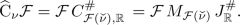  (7.5)

• (b) ${\widehat{{{\,\textrm{C}\,}}}}^\#_{\nu }$ can be extended to a conjugation on $L^2({\mathbb {R}})$ if and only if $\nu$ is a tempered distribution and ${\mathcal {F}}(\nu )$ is a unimodular function. Moreover,

  

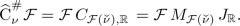  (7.6)

Proof

If ${\widehat{{{\,\textrm{C}\,}}}}_{\nu }$ is a conjugation, then by Proposition 7.7, $\nu \in {\mathcal {S}}'$ and

$$\begin{aligned} {\widetilde{C}}_{\mathbb {R}}:L^2({\mathbb {R}})\ni h \mapsto {\mathcal {F}}^{-1}{\widehat{{{\,\textrm{C}\,}}}}_{\nu }{\mathcal {F}}h \in L^2({\mathbb {R}})\end{aligned}$$

is also a conjugation since ${\mathcal {F}}$ is a unitary operator. Then, for any function $h \in {\mathcal {S}}$, $\nu *\overline{{\mathcal {F}}{h}}$ is well-defined since $\nu$ is tempered. Moreover, from Lemma 7.1 and (7.1) we have

This shows that ${\mathcal {F}}(\check{\nu })$ is a unimodular function and . Hence, by Theorem 5.9, function has to be even. Conversely, if $\nu \in {\mathcal {S}}'$ and ${\mathcal {F}}(\nu )$ is unimodular and even, then (7.5) defines an extension of ${\widehat{{{\,\textrm{C}\,}}}}_{\nu }$ and (a) is proved.

To see (b), we define

$$\begin{aligned} {\widetilde{C}}_{\mathbb {R}}:L^2({\mathbb {R}})\ni h \mapsto {\mathcal {F}}^{-1}{\widehat{{{\,\textrm{C}\,}}}}^\#_{\nu }{\mathcal {F}}h \in L^2({\mathbb {R}}). \end{aligned}$$

Similarly, the following equalities hold for $h\in {\mathcal {S}}$

$$\begin{aligned} {\widetilde{C}}_{\mathbb {R}}h&= {\mathcal {F}}^{-1}{\widehat{{{\,\textrm{C}\,}}}}^\#_{\nu }{\mathcal {F}}h = {\mathcal {F}}^{-1}\Big (\nu *\overline{\big ({\mathcal {F}}h\big )\check{}}\Big ) = {\mathcal {F}}\Big (\big (\nu *\Big (\overline{{\mathcal {F}}h}\Big )\check{}\big )\check{}\Big ) = {\mathcal {F}}\big (\check{\nu }*\big ({\mathcal {F}}\bar{\check{{h}}})\big ) \\&= {\mathcal {F}}(\check{\nu }) \cdot {\mathcal {F}}({\mathcal {F}}(\bar{\check{h}})) = {\mathcal {F}}(\check{\nu }) \cdot {\bar{h}}=C_{{\mathcal {F}}(\check{\nu }),{\mathbb {R}}}h. \end{aligned}$$

By (5.3), we get that ${\mathcal {F}}(\nu )$ is unimodular. $\square$

Remark 7.9

In order to define a conjugation, it is easier to start with a function - not a distribution. Indeed, let $\nu = {\mathcal {F}}(\Psi )$, where $\Psi \in L^\infty ({\mathbb {R}})$ is a unimodular function. Then $\nu \in {\mathcal {S}}'$ and

for every $\varphi \in {\mathcal {D}}$. Thus ${\mathcal {F}}(\check{\nu })=\Psi$ is unimodular. In such case ${\widehat{{{\,\textrm{C}\,}}}}^\#_{\nu }$ is a conjugation and

$$\begin{aligned} {\widehat{{{\,\textrm{C}\,}}}}^\#_{\nu }f = {\mathcal {F}}(\Psi ) *\bar{\check{{f}}}, \quad f \in {\mathcal {D}}. \end{aligned}$$

If in addition $\Psi$ is even, then ${\mathcal {F}}(\nu )$ is also even. Then ${\widehat{{{\,\textrm{C}\,}}}}_{\nu }$ is also a conjugation and

$$\begin{aligned} {\widehat{{{\,\textrm{C}\,}}}}_{\nu }f = {\mathcal {F}}(\Psi )*{\bar{f}}, \quad f \in {\mathcal {D}}. \end{aligned}$$

Now, we will use Remark 7.9 to present a few examples of conjugations, which may be treated as a convolution of the Fourier transform of a unimodular function with another function. The first example comes from one of the simplest unimodular functions one may think of.

Example 7.10

Let $\Psi ={{\,\textrm{sgn}\,}}$. Then $\Psi$ is unimodular and its Fourier transform is equal to [12, Exercise 5.11]

$$\begin{aligned} {\mathcal {F}}(\Psi ) = -i\sqrt{\tfrac{2}{\pi }}{{\,\mathrm{P.V.}\,}}\Big (\tfrac{1}{x}\Big ), \end{aligned}$$

where $\text {P. V.}$ denotes the principal value of a function. Finally,

$$\begin{aligned} {\widehat{{{\,\textrm{C}\,}}}}^\#_{{\mathcal {F}}(\Psi )} (f) = -i\sqrt{\tfrac{2}{\pi }}{{\,\mathrm{P.V.}\,}}\Big (\tfrac{1}{x}\Big ) *\bar{\check{{f}}} = -i\sqrt{2\pi } \frac{1}{\pi }{{\,\mathrm{P.V.}\,}}\Big (\tfrac{1}{x}\Big ) *\bar{\check{{f}}} = -i\, {\mathcal {H}}(\bar{\check{{f}}}), \quad f\in {\mathcal {D}}, \end{aligned}$$

where ${\mathcal {H}}$ is the Hilbert transform (see [7, Problem 14.49]¹).

Example 7.11

Let $\Psi =2\chi _{[-a,a]}-1$ for $a>0$. Then $\Psi$ is even and unimodular and from [7, Example 14.1]

$$\begin{aligned} {\mathcal {F}}(\Psi ) = \frac{4 \sin (ax)}{\sqrt{2\pi }x} - \delta _0 = \frac{4a{{\,\textrm{sinc}\,}}(ax)}{\sqrt{2\pi }}-\delta _0. \end{aligned}$$

Hence, for any $f \in {\mathcal {D}}$,

$$\begin{aligned} {\widehat{{{\,\textrm{C}\,}}}}^\#_{{\mathcal {F}}(\Psi )} (f)&=\frac{4a{{\,\textrm{sinc}\,}}(ax)}{\sqrt{2\pi }} *\bar{\check{{f}}}- \delta _0 *\bar{\check{{f}}} = \tfrac{2\sqrt{2}a}{\sqrt{\pi }}\,{{\,\textrm{sinc}\,}}(ax) *\bar{\check{{f}}}- \overline{f(0)}, \\ {\widehat{{{\,\textrm{C}\,}}}}_{{\mathcal {F}}(\Psi )} (f)&=\frac{4a{{\,\textrm{sinc}\,}}(ax)}{\sqrt{2\pi }} *{{\bar{f}}}- \delta _0 *{{\bar{f}}} = \tfrac{2\sqrt{2}a}{\sqrt{\pi }}\,{{{\,\textrm{sinc}\,}}(ax)} *{{\bar{f}}}- \overline{f(0)}. \end{aligned}$$

Example 7.12

Let $a>0$ and $\Psi (x)=e^{-iax^2}$, $x\in {\mathbb {R}}$. Then

$$\begin{aligned} {\mathcal {F}}(\Psi )=\tfrac{1}{\sqrt{2a}}\ e^{\frac{x^2}{4a}-\frac{\pi }{4}}. \end{aligned}$$

Thus, for $f \in {\mathcal {D}}$,

$$\begin{aligned} {\widehat{{{\,\textrm{C}\,}}}}^\#_{{\mathcal {F}}(\Psi )} (f)&=\tfrac{1}{\sqrt{2a}}\ e^{\frac{x^2}{4a}-\frac{\pi }{4}}*\bar{\check{{f}}},\\ {\widehat{{{\,\textrm{C}\,}}}}_{{\mathcal {F}}(\Psi )} (f)&=\tfrac{1}{\sqrt{2a}}\ e^{\frac{x^2}{4a}-\frac{\pi }{4}}*{\bar{f}}. \end{aligned}$$

Example 7.13

Let $\Psi (t)={{\,\textrm{sgn}\,}}(\cos \,t)$. Then $\Psi$ is a unimodular even function. Since ${\mathcal {F}}(\chi _{[a,b]})=i\frac{e^{-ibx}-e^{-iax}}{\sqrt{2\pi }x}$ [7, Example 14.1] for every a, $b\in {\mathbb {R}}$, $a<b$, by the dominated convergence theorem and the definition of the Fourier transform for any $\varphi \in {\mathcal {S}}$ we get

$$\begin{aligned} \left[ {\mathcal {F}}({{\,\textrm{sgn}\,}}(\cos t))\right] (\varphi )&= \frac{1}{\sqrt{2\pi }}\int _{\mathbb {R}}{{\,\textrm{sgn}\,}}(\cos t) \cdot {\mathcal {F}}(\varphi ) dx \\&= \frac{1}{\sqrt{2\pi }}\sum _{k \in {\mathbb {Z}}}\int _{-\frac{\pi }{2}+k\pi }^{\frac{\pi }{2}+k\pi } (-1)^k \cdot {\mathcal {F}}(\varphi ) dx \\ {}&= \sum _{k \in {\mathbb {Z}}}(-1)^k \frac{1}{\sqrt{2\pi }} \int _{\mathbb {R}}\chi _{[-\frac{\pi }{2} +k\pi ,\frac{\pi }{2} +k\pi ]} \cdot {\mathcal {F}}(\varphi )dx\\&= \sum _{k \in {\mathbb {Z}}}(-1)^k \left[ {\mathcal {F}}(\chi _{[-\frac{\pi }{2} +k\pi ,\frac{\pi }{2} +k\pi ]}) \right] (\varphi )\\&= \frac{1}{2\pi }\sum _{k \in {\mathbb {Z}}}(-1)^k \int _{\mathbb {R}}2 {{\,\textrm{sinc}\,}}\big (\tfrac{\pi }{2} x\big ) \cdot e^{-ikx} \cdot \varphi (x) dx. \end{aligned}$$

Hence

$$\begin{aligned} {\widehat{{{\,\textrm{C}\,}}}}^\#_{{\mathcal {F}}(\Psi )} (f) = \frac{2}{\sqrt{\pi }}\left( \sum _{k \in {\mathbb {Z}}}(-1)^k {{\,\textrm{sinc}\,}}\bigg (\tfrac{\pi }{2} x\bigg ) e^{-ikx}\right) *\bar{\check{{f}}}, \quad f \in {\mathcal {S}}. \end{aligned}$$

The next proposition shows that operators ${\widehat{{{\,\textrm{C}\,}}}}^\#_{\nu }$ and ${\widehat{{{\,\textrm{C}\,}}}}_{\nu }$, which are defined in terms of convolution, satisfy some commuting relations with translation operators.

Proposition 7.14

Let $x\in {\mathbb {R}}$. For conjugations ${\widehat{{{\,\textrm{C}\,}}}}^\#_{\nu }$, ${\widehat{{{\,\textrm{C}\,}}}}_{\nu }$ the following holds:

• (a) $\tau _x {\widehat{{{\,\textrm{C}\,}}}}^\#_{\nu }={\widehat{{{\,\textrm{C}\,}}}}^\#_{\nu }\tau _{-x}$,

• (b) $\tau _x {\widehat{{{\,\textrm{C}\,}}}}_{\nu }={\widehat{{{\,\textrm{C}\,}}}}_{\nu }\tau _{x}$.

In particular, $\tau _x J^\#_{\mathbb {R}}=J^\#_{\mathbb {R}}\tau _{-x}$ and $\tau _x J_{\mathbb {R}}=J_{\mathbb {R}}\tau _{x}$.

Proof

Let $f\in {\mathcal {D}}$. Then, for every $t \in {\mathbb {R}}$, we have

$$\begin{aligned} (\tau _x {\widehat{{{\,\textrm{C}\,}}}}^\#_{\nu }\tau _x f)(t)&= \big ({\widehat{{{\,\textrm{C}\,}}}}^\#_{\nu }\tau _x f\big )(t-x) = \big (\nu *\overline{\check{\tau _x f}}\big )(t-x) \\&= \nu \Big (\tau _{t-x} \big (\check{\overline{\check{\tau _x f}}}\big )\Big )= \nu (\tau _{t-x} \overline{\tau _x f}) = \nu (\tau _t {\bar{f}}) = (\nu *\bar{\check{{f}}})(t) = ({\widehat{{{\,\textrm{C}\,}}}}^\#_{\nu }f) (t) \end{aligned}$$

and

$$\begin{aligned} (\tau _x {\widehat{{{\,\textrm{C}\,}}}}_{\nu }\tau _{-x} f)(t)&= \big ({\widehat{{{\,\textrm{C}\,}}}}_{\nu }\tau _{-x} f\big )(t-x) = \big (\nu *\overline{\tau _{-x} f}\big )(t-x) \\&= \nu \Big (\tau _{t-x} \big (\overline{\check{\tau _{-x} f}}\big )\Big )= \nu (\tau _{t-x} \overline{\tau _x \check{f}}) = \nu (\tau _t \bar{\check{{f}}}) = (\nu *{\bar{f}})(t) = ({\widehat{{{\,\textrm{C}\,}}}}_{\nu }f) (t) \end{aligned}$$

which gives the claim. $\square$

Now, we are ready to characterize all conjugations on ${\mathbb {R}}$ that satisfy commuting relations with translations.

Theorem 7.15

Let ${\widehat{{{\,\textrm{C}\,}}}}$ be a conjugation on $L^2({\mathbb {R}})$. Then

• (a) $\tau _x{\widehat{{{\,\textrm{C}\,}}}}={\widehat{{{\,\textrm{C}\,}}}}\tau _{-x}$ for all $x\in {\mathbb {R}}$ if and only if there exists a unimodular function $\Psi \in L^\infty ({\mathbb {R}})$ such that ${\widehat{{{\,\textrm{C}\,}}}}= {\widehat{C}}^\#_{{\mathcal {F}}(\Psi )}={\mathcal {F}}(\Psi )*J^\#_{\mathbb {R}}$,

• (b) $\tau _x{\widehat{{{\,\textrm{C}\,}}}}={\widehat{{{\,\textrm{C}\,}}}}\tau _{x}$ for all $x\in {\mathbb {R}}$ if and only if there exists a unimodular even function $\Psi \in L^\infty ({\mathbb {R}})$ such that ${\widehat{{{\,\textrm{C}\,}}}}= {\widehat{C}}_{{\mathcal {F}}(\Psi )}={\mathcal {F}}(\Psi )*J_{\mathbb {R}}$.

Proof

The equality $\tau _x{\widehat{{{\,\textrm{C}\,}}}}={\widehat{{{\,\textrm{C}\,}}}}\tau _{-x}$, $x\in {\mathbb {R}}$, combined with Lemma 7.1 (c), gives us

$$\begin{aligned} M_{G_x}{\mathcal {F}}^{-1}{\widehat{{{\,\textrm{C}\,}}}}{\mathcal {F}}={\mathcal {F}}^{-1}\tau _x{\widehat{{{\,\textrm{C}\,}}}}{\mathcal {F}}={\mathcal {F}}^{-1}{\widehat{{{\,\textrm{C}\,}}}}\tau _{-x}{\mathcal {F}}={\mathcal {F}}^{-1}{\widehat{{{\,\textrm{C}\,}}}}{\mathcal {F}}M_{G_{-x}}, \quad x \in {\mathbb {R}}. \nonumber \\ \end{aligned}$$

(7.7)

By Theorem 5.8, there exists a unimodular function $\Psi \in L^\infty ({\mathbb {R}})$ such that

$$\begin{aligned} {\mathcal {F}}^{-1}{\widehat{{{\,\textrm{C}\,}}}}{\mathcal {F}}=M_{\Psi }J_{\mathbb {R}}. \end{aligned}$$

On the other hand, by Theorem 7.8(b), $\widehat{C}^\#_{{\mathcal {F}}(\Psi )}{\mathcal {F}}={\mathcal {F}}M_\Psi J_{\mathbb {R}}$. Hence, $\widehat{C}^\#_{{\mathcal {F}}(\Psi )}={\widehat{{{\,\textrm{C}\,}}}}$, which gives us the first part of the equivalence in (a). The second part of the equivalence in (a) is guaranteed by Proposition 7.14.

In order to prove (b), we show that

$$\begin{aligned} M_{G_x}{\mathcal {F}}^{-1}{\widehat{{{\,\textrm{C}\,}}}}{\mathcal {F}}={\mathcal {F}}^{-1}{\widehat{{{\,\textrm{C}\,}}}}{\mathcal {F}}M_{G_{x}}, \quad x\in {\mathbb {R}}\end{aligned}$$

(7.8)

and then, similarly as in the proof of (a), we use Theorem 5.9, Theorem 7.8, and Proposition 7.14. $\square$

Remark 7.16

A bounded linear operator $\Phi$ on $L^2({\mathbb {R}})$ is called a stationary filter if

$$\begin{aligned} \Phi \tau _s = \tau _s \Phi \quad \text {for every } s\in {\mathbb {R}}. \end{aligned}$$

It was shown (see [18, Section 7.5.3(c)]) that such operator is a convolution operator, i.e., $\Phi f=\nu *f$ for $f\in L^2({\mathbb {R}})$, where $\nu$ is a tempered distribution. The idea of the proof of the aforementioned property consisted of the following steps

• transform $\Phi$ to $M = {\mathcal {F}}\Phi {\mathcal {F}}^{-1}$

• transfer the operator M to the unit circle by taking $U_2M U_2^{-1}$,

• use the description of the commutant of the multiplication operator $M_z$ on the unit circle.

The description of the commutant of $M_z$ was also a main tool in the proof of [4, Theorem 2.2 and Theorem 2.4], which was a starting point in our paper. We used the transformation $\widetilde{U}_2$ and the Fourier transform ${\mathcal {F}}$ to characterize conjugations on $L^2({\mathbb {R}})$ in Theorems 5.8, 5.9, 7.8 and 7.15. On the other hand, it is also possible to obtain some of these theorems by applying [18, Section 7.5.3(c)].

Indeed, we will show that Theorem 7.15 can be obtained in a different way. Assume that

$$\begin{aligned} \Phi _1&={\widehat{{{\,\textrm{C}\,}}}}_1 J^\#_{\mathbb {R}}, \text { where } {\widehat{{{\,\textrm{C}\,}}}}_1 \text { satisfies condition }\tau _x {\widehat{{{\,\textrm{C}\,}}}}_1 = {\widehat{{{\,\textrm{C}\,}}}}_1 \tau _{-x},\, x\in {\mathbb {R}},\\ \Phi _2&={\widehat{{{\,\textrm{C}\,}}}}_2 J_{\mathbb {R}}, \text { where } {\widehat{{{\,\textrm{C}\,}}}}_2 \text { satisfies condition } \tau _x {\widehat{{{\,\textrm{C}\,}}}}_2 = {\widehat{{{\,\textrm{C}\,}}}}_2 \tau _{x},\, x\in {\mathbb {R}}. \end{aligned}$$

Then $\Phi _1$, $\Phi _2$ are bounded linear operators on $L^2({\mathbb {R}})$. For any $x\in {\mathbb {R}}$ the following holds

$$\begin{aligned} \tau _x\Phi _1&= \tau _x{\widehat{{{\,\textrm{C}\,}}}}_1 J^\#_{\mathbb {R}}={\widehat{{{\,\textrm{C}\,}}}}_1\tau _{-x} J^\#_{\mathbb {R}}={\widehat{{{\,\textrm{C}\,}}}}_1 J^\#_{\mathbb {R}}\tau _x=\Phi _1 \tau _x, \\ \tau _x\Phi _2&=\tau _x{\widehat{{{\,\textrm{C}\,}}}}_2 J_{\mathbb {R}}={\widehat{{{\,\textrm{C}\,}}}}_2\tau _{x} J_{\mathbb {R}}={\widehat{{{\,\textrm{C}\,}}}}_2 J_{\mathbb {R}}\tau _x=\Phi _2 \tau _x . \end{aligned}$$

Theorem [18, Section 7.5.3(c)] guarantees that there are distributions $\nu _1$, $\nu _2$ such that $\nu _1={\mathcal {F}}(\Psi _1)$, $\nu _2={\mathcal {F}}(\Psi _2)$, for some $\Psi _1$, $\Psi _2\in L^\infty ({\mathbb {R}})$, and

$$\begin{aligned} \Phi _1 f=\nu _1*f\quad \text {and}\quad \Phi _2 f=\nu _2*f\quad \text {for}\ f\in {\mathcal {S}}. \end{aligned}$$

Since $J_{\mathbb {R}}$, $J^\#_{\mathbb {R}}$ are conjugations, for $f\in {\mathcal {S}}$, we have

$$\begin{aligned} {\widehat{{{\,\textrm{C}\,}}}}_1 f&=\Phi _1 J^\#_{\mathbb {R}}f=\Phi _1(\bar{\check{f}})= \nu _1*\bar{\check{f}} ={\mathcal {F}}(\Psi _1)*\bar{\check{f}},\\ {\widehat{{{\,\textrm{C}\,}}}}_2 f&=\Phi _2 J_{\mathbb {R}}f=\Phi _2({\bar{f}})= \nu _2*{\bar{f}} ={\mathcal {F}}(\Psi _2)*{\bar{f}}. \end{aligned}$$

Now, using for example the Fourier transform, we can show the appropriate attributes of $\Psi _1$ and $\Psi _2$.

An application of Theorem 7.15 gives the following two propositions characterizing conjugations on $L^2({\mathbb {R}})$ commuting (intertwining) with translations, which map one $L^2$ space on an interval into another $L^2$ space on an interval.

Proposition 7.17

Let ${\widehat{{{\,\textrm{C}\,}}}}$ be a conjugation on $L^2({\mathbb {R}})$ such that $\tau _x{\widehat{{{\,\textrm{C}\,}}}}={\widehat{{{\,\textrm{C}\,}}}}\tau _{-x}$ for all $x\in {\mathbb {R}}$. Assume that $a_1<b_1$. Then

$$\begin{aligned} {\widehat{{{\,\textrm{C}\,}}}}\Big (L^2(a_1, b_1)\Big )\subset L^2(a_2,b_2) \end{aligned}$$

(7.9)

if and only if

$$\begin{aligned} b_1-a_1\leqslant b_2-a_2 \text { and } {\widehat{{{\,\textrm{C}\,}}}}=\delta _\mu *J^\#_{\mathbb {R}}\text { for some } \mu \in [a_2+b_1, a_1+b_2]. \end{aligned}$$

In particular, if $b_1-a_1=b_2-a_2$, then the conjugation ${\widehat{{{\,\textrm{C}\,}}}}$ is unique and ${\widehat{{{\,\textrm{C}\,}}}}=\delta _{b_1+a_2}*J^\#_{\mathbb {R}}$.

Proof

For $\lambda >0$ let us consider the model space

$$\begin{aligned} K_{G_\lambda }=H^2({\mathbb {C}}_+)\ominus G_{\lambda }H^2({\mathbb {C}}_+)\subset L^2({\mathbb {R}}). \end{aligned}$$

Recall that ${\mathcal {F}}H^2({\mathbb {C}}_+)=L^2(0,\infty )$. Then, by Lemma 7.1,

$$\begin{aligned} {\mathcal {F}}G_{\lambda } H^2({\mathbb {C}}_+)=\tau _\lambda {\mathcal {F}}H^2({\mathbb {C}}_+)=\tau _\lambda L^2(0,\infty )=L^2(\lambda ,\infty ). \end{aligned}$$

Thus ${\mathcal {F}}K_{G_\lambda }= L^2(0,\lambda )$. In addition, Lemma 7.1 gives us

$$\begin{aligned} {\mathcal {F}}G_\mu K_{G_\lambda }= \tau _\mu {\mathcal {F}}K_{G_\lambda }= \tau _\mu L^2(0,\lambda )= L^2(\mu ,\mu +\lambda ) \end{aligned}$$

for any $\mu \in {\mathbb {R}}$.

Now, we apply Theorem 7.15 to ${\widehat{{{\,\textrm{C}\,}}}}$ and get a unimodular function $\Psi \in L^\infty ({\mathbb {R}})$ such that ${\widehat{{{\,\textrm{C}\,}}}}={\mathcal {F}}(\Psi )*J^\#_{\mathbb {R}}$. Hence, by Theorem 7.8, the following holds

$$\begin{aligned} {\mathcal {F}}^{-1}{\widehat{{{\,\textrm{C}\,}}}}\big (L^2(a_1, b_1)\big )&= {\mathcal {F}}^{-1}\big ({\mathcal {F}}(\Psi )*J^\#_{\mathbb {R}}\big ){\mathcal {F}}{\mathcal {F}}^{-1} L^2\big (a_1, a_1+(b_1-a_1)\big ) \\ {}&= C_{\Psi ,{\mathbb {R}}} G_{a_1}K_{G_{b_1- a_1}}. \end{aligned}$$

On the other hand, ${\mathcal {F}}^{-1} L^2(a_2, b_2)= G_{a_2}K_{G_{b_2- a_2}}$ and therefore inclusion (7.9) is equivalent to

$$\begin{aligned} C_{\Psi ,{\mathbb {R}}} \Big (G_{a_1}K_{G_{b_1- a_1}}\Big ) \subset G_{a_2}K_{G_{b_2- a_2}}. \end{aligned}$$

Example 6.5 shows that this is possible if and only if $b_1-a_1\leqslant b_2-a_2$. If so $\Psi =G_{\mu }$ for some $a_2+b_1\leqslant \mu \leqslant a_1+b_2$. Finally, since ${\mathcal {F}}(G_{\mu })=\delta _\mu$, we get ${\widehat{{{\,\textrm{C}\,}}}}=\delta _\mu *J^\#_{\mathbb {R}}$. The reverse implication is clear. $\square$

Proposition 7.18

Let ${\widehat{{{\,\textrm{C}\,}}}}$ be a conjugation on $L^2({\mathbb {R}})$ such that $\tau _x{\widehat{{{\,\textrm{C}\,}}}}={\widehat{{{\,\textrm{C}\,}}}}\tau _{x}$ for all $x\in {\mathbb {R}}$. Assume that $a_1<b_1$. Then

$$\begin{aligned} {\widehat{{{\,\textrm{C}\,}}}}\Big (L^2(a_1, b_1)\Big )\subset L^2(a_2,b_2) \end{aligned}$$

(7.10)

if and only if $a_2\leqslant a_1<b_1\leqslant b_2$ and ${\widehat{{{\,\textrm{C}\,}}}}=J^\#_{\mathbb {R}}$.

Proof

As above, by Theorem 7.15, there is a unimodular even function $\Psi \in L^\infty ({\mathbb {R}})$ such that ${\widehat{{{\,\textrm{C}\,}}}}={\mathcal {F}}(\Psi )*J_{\mathbb {R}}$. By Theorem 7.8, we have

$$\begin{aligned} {\mathcal {F}}^{-1}{\widehat{{{\,\textrm{C}\,}}}}(L^2(a_j, b_j)){} & {} ={\mathcal {F}}^{-1}\big ({\mathcal {F}}(\Psi )*J_{\mathbb {R}}\big ){\mathcal {F}}{\mathcal {F}}^{-1} L^2(a_j, a_j +(b_j- a_j))\\ {}{} & {} =C^\#_{\Psi ,{\mathbb {R}}} G_{a_j}K_{G_{b_j- a_j}} \end{aligned}$$

for $j=1,2$. Hence (7.10) is equivalent to

$$\begin{aligned} C^\#_{\Psi ,{\mathbb {R}}} \Big (G_{a_1}K_{G_{b_1- a_1}}\Big ) \subset G_{a_2}K_{G_{b_2- a_2}}. \end{aligned}$$

Now, by Example 6.10, any such $C^\#_{\Psi ,{\mathbb {R}}}$ (equivalently ${\widehat{{{\,\textrm{C}\,}}}}$) exists if and only if $a_2\leqslant a_1<b_1\leqslant b_2$ and ${\widehat{{{\,\textrm{C}\,}}}}=J^\#_{\mathbb {R}}$. Again, the reverse implication is clear.$\square$

8 Kernels of Wiener-Hopf Operators

Let $\Psi \in L^\infty ({\mathbb {R}})$. Following [18, Part B, Section 4.6.4], we define the Wiener-Hopf operator with a symbol $\Psi$ by the formula

$$\begin{aligned} (W_\Psi f)(x){} & {} = \chi _{{\mathbb {R}}_+} ({\mathcal {F}}( \Psi ) *f)(x)\\{} & {} = \int _{{\mathbb {R}}_+} ({\mathcal {F}}(\Psi ))(x-y) f(y) \text {d}y, \quad x \in {\mathbb {R}}_+, \quad f \in L^2({\mathbb {R}}_+). \end{aligned}$$

It is worth to notice that Toeplitz operators and Wiener-Hopf operators are unitarily equivalent, i.e.

$$\begin{aligned} W_\Psi = {\mathcal {F}}T_\Psi {\mathcal {F}}^{-1},\quad \Psi \in L^\infty ({\mathbb {R}}). \end{aligned}$$

In other words the following diagram commutes

In particular, $\ker W_\Psi = {\mathcal {F}}(\ker T_\Psi )$. Consequently, the following lemma holds.

Lemma 8.1

Let ${\widehat{{{\,\textrm{C}\,}}}}$ be a conjugation on $L^2({\mathbb {R}})$ and let $\Psi _1$, $\Psi _2 \in L^\infty ({\mathbb {R}})$. Then ${\widehat{{{\,\textrm{C}\,}}}}(\ker T_{\Psi _1}) \subset \ker (T_{\Psi _2})$ if and only if ${\mathcal {F}}{\widehat{{{\,\textrm{C}\,}}}}{\mathcal {F}}^{-1} (\ker W_{\Psi _1}) \subset \ker W_{\Psi _2}$.

Combining Theorem 6.3 and Theorem 6.8 with Lemma 8.1, we get the following two theorems.

Theorem 8.2

Let $H_1$, $H_2$ be unimodular functions in $L^\infty ({\mathbb {R}})$, such that $\ker W_{H_1}\ne \{0\}$. Let ${\widehat{{{\,\textrm{C}\,}}}}$ be a conjugation on $L^2({\mathbb {R}})$ satisfying

$$\begin{aligned} \tau _x {\widehat{{{\,\textrm{C}\,}}}}= {\widehat{{{\,\textrm{C}\,}}}}\tau _{-x} \text { for any }x >0. \end{aligned}$$

Then the following conditions are equivalent:

• (a) ${\widehat{{{\,\textrm{C}\,}}}}(\ker W_{H_1}) \subset \ker W_{H_2}$,

• (b) $H_2\leqslant H_1$ and ${\widehat{{{\,\textrm{C}\,}}}}= {\widehat{{{\,\textrm{C}\,}}}}^\#_{{\mathcal {F}}(B)}={\mathcal {F}}(B)* J_{{\mathbb {R}}}^\#$, where $\overline{H_1} \leqslant B \leqslant \overline{H_2}$.

Theorem 8.3

Let $H_1$, $H_2$ be unimodular functions in $L^\infty ({\mathbb {R}})$, such that $\ker W_{H_1}\ne \{0\}$. Let ${\widehat{{{\,\textrm{C}\,}}}}$ be a conjugation on $L^2({\mathbb {R}})$ such that

$$\begin{aligned} \tau _x {\widehat{{{\,\textrm{C}\,}}}}= {\widehat{{{\,\textrm{C}\,}}}}\tau _{x}\quad \text { for any }\ \ x >0. \end{aligned}$$

Then the following conditions are equivalent:

• (a) ${\widehat{{{\,\textrm{C}\,}}}}(\ker W_{H_1}) \subset \ker W_{H_2}$,

• (b) $H_2^\#\leqslant H_1$ and ${\widehat{{{\,\textrm{C}\,}}}}=J_{{\mathbb {R}}}$.

References

Bender, C.M.: Making sense of non-Hermitian hamiltonians. Rep. Progr. Phys. 70(6), 947–1018 (2007)
Bender, C.M., Boettcher, S.: Real spectra in non-hermitian hamiltonians having \(\mathscr{P}\mathscr{T}\) symmetry. Phys. Rev. Lett. 80, 5243–5246 (1998)
Caliceti, E., Graffi, S., Maioli, M.: Perturbation theory of odd anharmonic oscillators. Commun. Math. Phys. 75(1), 51–66 (1980)
Câmara, C., Kliś-Garlicka, K., Łanucha, B., Ptak, M.: Conjugations in \(l^2\) and their invariants. Anal. Math. Phis. 10 (2020)
Câmara, C., Kliś-Garlicka, K., Ptak, M.: Asymmetric truncated toeplitz operators and conjugations. Filomat 33, 3697–3710 (2019)
Câmara, C., Partington, J.R.: Toeplitz Kernels and Model Spaces, The Diversity and Beauty of Applied Operator Theory. Oper. Theory Adv. Appl., vol. 465, pp. 139–153. Birkhäuser/Springer, Cham (2018). https://doi.org/10.1007/978-3-319-75996-8_7
Duistermaat, J.J., Kolk, J.A.C.: Distributions. Theory and Applications. Birkhäuser Boston Inc, Boston, MA (2010)
Dymek, P., Płaneta, A., Ptak, M.: Conjugations Preserving Toeplitz Kernels. Integr. Eq. Oper. Theory 94, 39 (2022). https://doi.org/10.1007/s00020-022-02714-3
Garcia, S.R., Mashreghi, J., Ross, W.T.: Introduction to Model Spaces and Their Operators. Cambridge Studies in Advanced Mathematics. Cambridge University Press, Cambridge (2016)
Garcia, S.R., Prodan, E., Putinar, M.: Mathematical and physical aspects of complex symmetric operators. J. Phis. A, Math Theor 47, 1–54 (2014)
Garcia, S.R., Putinar, M.: Complex symmetric operators and applications. Trans. Amer. Math. Soc. 358, 1285–1315 (2006)
Grubb, G.: Distributions and Operators. Springer, New York, NY (2009)
King, F.W.: Hilbert Transforms. Encyclopedia of Mathematics and its Applications, vol. 1. Cambridge University Press, Cambridge (2009)
King, F.W.: Hilbert Transforms. Encyclopedia of Mathematics and its Applications, vol. 2. Cambridge University Press, Cambridge (2009)
Kuzhel’, S.O., Patsyuk, O.M.: On the theory of pt-symmetric operators. Ukrainian Math. J. 64, 35–55 (2012)
Makarov, N., Poltoratski, A.: Meromorphic inner functions, toeplitz kernels and the uncertainty principle, perspectives in analysis. Math. Phys. Stud. 27, 185–252 (2005)
Młocek, W., Ptak, M.: On the reflexivity of subspaces of toeplitz operators on the hardy space on the upper half-plane. Czechoslovak Math. J. 63, 421–434 (2013)
Nikolski, N.K.: Operators, Functions, and Systems: An Easy Reading, Volume I: Hardy, Hankel, and Toeplitz. Mathematical Surveys and Monographs, vol. 92. American Mathematical Society, Providence, RI (2002)
Rosenblum, M., Rovnyak, J.: Topics in Hardy Classes and Univalent Functions. Birkhäuser Verlag, Basel, Basel (1994)
Rudin, W.: Functional Analysis. McGraw-Hill Inc, New York, New York NY (1991)
Sarason, D.: Algebraic properties of truncated toeplitz operators. Operat. Matrices 1, 491–526 (2007)
Schmüdgen, K.: Unbounded Self-adjoint Operators on Hilbert Space. Graduate Texts in Mathematics, vol. 265. Springer, Dordrecht (2012)
Sz.-Nagy, B., Foias, C., Bercovici, H., Kérchy, L.: Harmonic analysis of operators on hilbert space. Springer, New York, NY (2010)
Funding
The authors declare that no funds, grants, or other support were received during the preparation of this manuscript.
Author information
Authors and Affiliations
Corresponding author
Ethics declarations
Conflict of interest
The authors have no relevant financial or non-financial interests to disclose.
Additional information
Publisher's Note
Springer Nature remains neutral with regard to jurisdictional claims in published maps and institutional affiliations.
Rights and permissions
Open Access This article is licensed under a Creative Commons Attribution 4.0 International License, which permits use, sharing, adaptation, distribution and reproduction in any medium or format, as long as you give appropriate credit to the original author(s) and the source, provide a link to the Creative Commons licence, and indicate if changes were made. The images or other third party material in this article are included in the article’s Creative Commons licence, unless indicated otherwise in a credit line to the material. If material is not included in the article’s Creative Commons licence and your intended use is not permitted by statutory regulation or exceeds the permitted use, you will need to obtain permission directly from the copyright holder. To view a copy of this licence, visit http://creativecommons.org/licenses/by/4.0/.
About this article
Cite this article
Dymek, P., Płaneta, A. & Ptak, M. Conjugations on \(L^2\) Space on the Real Line. Results Math 79, 39 (2024). https://doi.org/10.1007/s00025-023-02046-7
Received:
Accepted:
Published:
DOI: https://doi.org/10.1007/s00025-023-02046-7