Performance Benchmarking of Tsunami-HySEA Model for NTHMP’s Inundation Mapping Activities

Abstract

The Tsunami-HySEA model is used to perform some of the numerical benchmark problems proposed and documented in the “Proceedings and results of the 2011 NTHMP Model Benchmarking Workshop”. The final aim is to obtain the approval for Tsunami-HySEA to be used in projects funded by the National Tsunami Hazard Mitigation Program (NTHMP). Therefore, this work contains the numerical results and comparisons for the five benchmark problems (1, 4, 6, 7, and 9) required for such aim. This set of benchmarks considers analytical, laboratory, and field data test cases. In particular, the analytical solution of a solitary wave runup on a simple beach, and its laboratory counterpart, two more laboratory tests: the runup of a solitary wave on a conically shaped island and the runup onto a complex 3D beach (Monai Valley) and, finally, a field data benchmark based on data from the 1993 Hokkaido Nansei-Oki tsunami.

1 Introduction

According to the 2006 Tsunami Warning and Education Act, all inundation models used in National Tsunami Hazard Mitigation Program (NTHMP) projects must meet benchmarking standards and be approved by the NTHMP Mapping and Modeling Subcommittee (MMS). To this end, a workshop was held in 2011 by the MMS, and participating models whose results were approved for tsunami inundation modeling were documented in the “Proceedings and results of the 2011 NTHMP Model Benchmarking Workshop” (NTHMP 2012). Since then, other models have been subjected to the benchmark problems used in the workshop, and their approval and use subsequently requested for NTHMP projects. For those currently wishing to benchmark their tsunami inundation models, a first step consists of completing benchmark problems 1, 4, 6, 7, and 9 in NTHMP (2012). This is the aim of the present benchmarking study for the case of the Tsunami-HySEA model. Another preliminary requirement for achieving MMS approval for tsunami inundation models is that all models being used by US federal, state, territory, and commonwealth governments should be provided to the public as open source. A freely accessible open source version of Tsunami-HySEA can be downloaded from the website https://edanya.uma.es/hysea.

Besides NTHMP (2012) and references therein, for NTHMP-benchmarked tsunami models, other authors have performed similar benchmarking efforts as the one presented here with their particular models, as is the case of Nicolsky et al. (2011), Apotsos et al. (2011) or Tolkova (2014). In addition, a model intercomparison of eight NTHMP models for benchmarks 4 (laboratory simple beach) and 6 (conical island) can be found in the study by Horrillo et al. (2015).

2 The Tsunami-HySEA Model

HySEA (Hyperbolic Systems and Efficient Algorithms) software consists of a family of geophysical codes based on either single-layer, two-layer stratified systems or multilayer shallow-water models. HySEA codes have been developed by EDANYA Group (https://edanya.uma.es) from the Universidad de Málaga (UMA) for more than a decade and they are in continuous evolution and upgrading. Tsunami-HySEA is the numerical model specifically designed for tsunami simulations. It combines robustness, reliability, and good accuracy in a model based on a GPU faster than real-time (FTRT) implementation. It has been thoroughly tested, and in particular has passed not only all tests by Synolakis et al. (2008), but also other laboratory tests and proposed benchmark problems. Some of them can be found in the studies by Castro et al. (2005, 2006, 2012), Gallardo et al. (2007), de la Asunción et al. (2013), and NTHMP (2016).

2.1 Model Equations

Tsunami-HySEA solves the well-known 2D non-linear one-layer shallow-water system in both spherical and Cartesian coordinates. For the sake of brevity and simplicity, only the latter system is written:

$$\begin{aligned} \frac{\partial h}{\partial t} + \frac{{\partial \left( {hu} \right)}}{\partial x} + \frac{{\partial \left( {hv} \right)}}{\partial y} = 0, \hfill \\ \frac{{\partial \left( {hu} \right)}}{\partial t} + \frac{\partial }{\partial x}\left( {hu^{2} + \frac{1}{2}gh^{2} } \right) + \frac{{\partial \left( {huv} \right)}}{\partial y} = gh\frac{\partial H}{\partial x} + S_{x} , \hfill \\ \frac{\partial (hv)}{\partial t} + \frac{\partial }{\partial y}\left( {hv^{2} + \frac{1}{2}gh^{2} } \right) + \frac{{\partial \left( {huv} \right)}}{\partial x} = gh\frac{\partial H}{\partial y} + S_{y} . \hfill \\ \end{aligned}$$

In the previous set of equations, $h\left( {\varvec{x},t} \right)$ denotes the thickness of the water layer at point $\varvec{x} \in D \subset {\mathbb{R}}^{2}$ at time $t$, with $D$ being the horizontal projection of the 3D domain where tsunami takes place. $H\left( \varvec{x} \right)$ is the depth of the bottom at point $\varvec{x}$ measured from a fixed level of reference. $u\left( {\varvec{x},t} \right)$ and $v\left( {\varvec{x},t} \right)$ are the height-averaged velocity in the x- and y-directions, respectively, and g denotes gravity. Let us also define the function $\eta \left( {\varvec{x},\varvec{t}} \right) = h\left( {\varvec{x},t} \right) - H(\varvec{x})$ that corresponds to the free surface of the fluid.

The terms $S_{x}$ and $S_{y}$ parameterize the friction effects and two different laws are considered:

• 1. The Manning law:

  $$S_{x} = - \frac{{ghM_{n}^{2} u\|(u,v)\|}}{{h^{4/3} }},$$
  $$S_{y} = - \frac{{ghM_{n}^{2} v\|(u,v)\|}}{{h^{4/3} }},$$

where $M_{n} > 0$ is the manning coefficient.

• 2. A quadratic law:

  $$S_{x} = - c_{f} u \|(u,v)\|, S_{y} = - c_{f} v \|(u,v)\|,$$

where $c_{f} > 0$ is the friction coefficient. In all the numerical tests presented in this study the Manning law is used.

Finally, to perform the BP4 (runup in a simple beach-experimental) and BP6 (conical island), a version of the code including dispersion was used. Dispersive model equations are written as follows:

$$\begin{aligned} \frac{\partial h}{\partial t} + \frac{{\partial \left( {hu} \right)}}{\partial x} + \frac{{\partial \left( {hv} \right)}}{\partial y} = 0, \hfill \\ \frac{{\partial \left( {hu} \right)}}{\partial t} + \frac{\partial }{\partial x}\left( {hu^{2} + \frac{1}{2}gh^{2} + \frac{1}{2}hp} \right) + \frac{{\partial \left( {huv} \right)}}{\partial y} = (gh + p)\frac{\partial H}{\partial x} + S_{x} , \hfill \\ \frac{\partial (hv)}{\partial t} + \frac{\partial }{\partial y}\left( {hv^{2} + \frac{1}{2}gh^{2} + \frac{1}{2}hp} \right) + \frac{{\partial \left( {huv} \right)}}{\partial x} = (gh + p)\frac{\partial H}{\partial y} + S_{y} , \hfill \\ \frac{{\partial \left( {hw} \right)}}{\partial t} = p, \hfill \\ h\frac{\partial (hu)}{\partial x} - hu\frac{{\partial \left( {2\eta - h} \right)}}{\partial x} + h\frac{{\partial \left( {hv} \right)}}{\partial y} - hv\frac{{\partial \left( {2\eta - h} \right)}}{\partial y} + 2hw = 0. \hfill \\ \end{aligned}$$

The dispersive system implemented can be interpreted as a generalized Yamazaki model (Yamazaki et al. 2009) where the term $\frac{\partial h}{\partial t}w$ is not neglected in the equation for the vertical velocity. The free divergence equation has been multiplied by $h^{2}$ to write it with the conserved variables $hu$ and $hv$. In addition, due to the rewriting of the last equation, no special treatment is required in the presence of wet–dry fronts. The breaking criteria employed is similar to the criteria presented by Roeber et al. (2010), based on an “eddy viscosity” approach.

2.2 Numerical Solution Method

Tsunami-HySEA solves the two-dimensional shallow-water system using a high-order (second and third order) path-conservative finite-volume method. Values of $h, hu$ and $hv$ at each grid cell represent cell averages of the water depth and momentum components. The numerical scheme is conservative for both mass and momentum in flat bathymetries and, in general, is mass preserving for arbitrary bathymetries. High order is achieved by a non-linear total variation diminishing (TVD) reconstruction operator of the unknowns $h, hu, hv$ and $\eta = h - H$. Then, the reconstruction of $H$ is recovered using the reconstruction of $h$ and $\eta$. Moreover, in the reconstruction procedure, the positivity of the water depth is ensured. Tsunami-HySEA implements several reconstruction operators: MUSCL (Monotonic Upstream-Centered Scheme for Conservation Laws, see van Leer 1979) that achieves second order, the hyperbolic Marquina’s reconstruction (see Marquina 1994) that achieves third order, and a TVD combination of piecewise parabolic and linear 2D reconstructions that also achieves third order [see Gallardo et al. (2011)]. The high-order time discretization is performed using the second- or third-order TVD Runge–Kutta method described in Gottlieb and Shu (1998). At each cell interface, Tsunami-HySEA uses Godunov’s method based on the approximation of 1D projected Riemann problems along the normal direction to each edge. In particular Tsunami-HySEA implements a PVM-type (polynomial viscosity matrix) method that uses the fastest and the slowest wave speeds, similar to HLL (Harten–Lax–van Leer) method (see Castro and Fernández-Nieto 2012). A general overview of the derivation of the high-order methods is shown by Castro et al. 2009. For large computational domains and in the framework of Tsunami Early Warning Systems, Tsunami-HySEA also implements a two-step scheme similar to leap-frog for the deep-water propagation step and a second-order TVD-weighted averaged flux (WAF) flux-limiter scheme, described by de la Asunción et al. 2013, for close to coast propagation/inundation step. The combination of both schemes guaranties the mass conservation in the complete domain and prevents the generation of spurious high-frequency oscillations near discontinuities generated by leap-frog type schemes. At the same time, this numerical scheme reduces computational times compared with other numerical schemes, while the amplitude of the first tsunami wave is preserved.

Concerning the wet–dry fronts discretization, Tsunami-HySEA implements the numerical treatment described by Castro et al. (2005) and Gallardo et al. (2007) that consists of locally replacing the 1D Riemann solver used during the propagation step, by another 1D Riemann solver that takes into account the presence of a dry cell. Moreover, the reconstruction step is also modified to preserve the positivity of the water depth. The resulting schemes are well balanced for the water at rest, that is, they exactly preserve the water at rest solutions, and are second- or third-order accurate, depending on the reconstruction operator and the time stepping method. Finally, the numerical implementation of Tsunami-HySEA has been performed on GPU clusters (de la Asunción et al. 2011, 2013, Castro et al. 2011) and nested-grids configurations are available (Macías et al. 2013, 2014, 2015, 2016). These facts allow to speed up the computations, being able to perform complex simulations, in very large domains, much faster than real time (Macías et al. 2013, 2014, 2016).

The dispersive model implements a formal second-order well-balanced hybrid finite-volume/difference (FV/FD) numerical scheme. The non-hydrostatic system can be split into two parts: one corresponding to the non-linear shallow-water component in conservative form and the other corresponding to the non-hydrostatic terms. The hyperbolic part of the system is discretized using a PVM path-conservative finite-volume method (Castro and Fernández-Nieto 2012 and Parés 2006), and the dispersive terms are discretized with compact finite differences. The resulting ODE system in time is discretized using a TVD Runge–Kutta method (Gottlieb and Shu 1998).

3 Benchmark Problem Comparisons

This section contains the Tsunami-HySEA results for each of the five benchmark problems that are required by the NTHMP Tsunami Inundation Model Approval Process (July 2015). The specific version of Tsunami-HySEA code benchmarked in the present study is the second order with MUSCL reconstruction and its second-order dispersive counterpart when dispersion is required. Detailed descriptions of all benchmarks, as well as topography data when required and laboratory or field data for comparison when applicable, can be found in the repository of benchmark problems https://gitub.com/rjleveque/nthmp-benchmark-problems for NTHMP, or in the NCTR repository http://nctr.pmel.noaa.gov/benchmark/. Results from model participating in original 2011 workshop can be found at NTHMP (2012). For the sake of completeness, a brief description of each benchmark problem is provided. For BP#1 and BP#4, dealing with analytical solutions or very simple laboratory 1D configurations, non-dimensional variables are used everywhere. For problems dealing with 2D complex laboratory experiments (BP#6 and BP#7) scaled dimensional problems are solved. Finally, BP#9 dealing with field data is solved in real-world not-scaled dimensional variables.

3.1 Benchmark Problem #1: Simple Wave on a Simple Beach—analytical—CASE H/d = 0.019

In this section, we compare numerical results for solitary wave shoaling on a plane beach to an analytic solution based on the shallow-water equations. The benchmark data for comparison are obtained from NTHMP (2012) or Synolakis et al. (2008). In the present case, the model has been run in non-linear, non-dispersive, and no friction mode as requested for comparison and verification purposes. In this problem, the wave of height H is initially centered at distance L from the beach toe and the shape for the bathymetry consists of an area of constant depth d, connected to a plane sloping beach of angle β = arccot(19.85) as schematically shown in Fig. 1.

Fig. 1

Non-scaled sketch of a canonical 1D simple beach with a solitary wave (X ₀ = d cot β)

3.1.1 Problem Setup

Problem setup is defined by the following items (all the variables in this BP are non-dimensional and the computations have been performed in non-dimensional variables):

• Friction: no friction (as required).

• Parameters: d = 1, g = 1, and H = 0.019 (see Fig. 1 for d and H).

• Computational domain: the computational domain in x spanned from x = −10 to x = 70.

• Boundary conditions: a non-reflective boundary condition at the right side of the computational domain is imposed (beach slope is located to the left).

• Initial condition: the prescribed soliton at time t = 0 with the proposed correction for the initial velocity. These initial data were given by:

  $$\eta \left( {x,0} \right) = H { \sec }h^{2} (\gamma (x - {\text{X}}_{ 1} )/d),$$

  where $X_{1} = X_{0} + L$, with $L = {\text{arccosh}}(\sqrt {20} )/\gamma$ the half-length of the solitary wave, and $\gamma = \sqrt {3H/4d}$ the water wave elevation and

  $$u\left( {x,0} \right) = - \sqrt {\frac{g}{d}} \eta (x,0)$$

  for the initial velocity (the minus sign meaning approaching the coast, that in the numerical test is on the left-hand side).

• Grid resolution: the numerical results presented are for a computational mesh composed of 800 cells, i.e., Δx = 0.1 = d/10. For the convergence analysis of the maximum runup, two other increased resolutions have been used, Δx = 0.05 = d/20 and Δx = 0.025 = d/40 with 1600 and 3200 cells, respectively.

• Time stepping: variable time stepping based on a CFL condition is used.

• CFL: CFL number is set to 0.9.

• Versions of the code: Tsunami-HySEA third-order (with Marquina’s reconstruction) and second-order (with MUSCL reconstruction) models have been benchmarked using this particular problem. Both models give nearly identical results.

3.1.2 Tasks to be Performed

To accomplish this benchmark the following four tasks were suggested:

• 1. Numerically compute the maximum runup of the solitary wave.

• 2. Compare the numerically and analytically computed water level profiles at t = 25 (d/g)^1/2, t = 35 (d/g)^1/2, t = 45 (d/g)^1/2, t = 55 (d/g)^1/2, and t = 65 (d/g)^1/2. Note that as we used the MATLAB scripts and data provided by Juan Horrillo on behalf of the NTHMP, the numerical vs analytical comparison is performed at the times given in the provided data and depicted by the corresponding MATLAB script that does not correspond exactly with all the time instants given in BP1 description. More precisely, they do correspond to t = 35:5:65 (d/g)^1/2. Therefore, t = 25 (d/g)^1/2 is missing and t = 40, 50, and 60 (d/g)^1/2 are shown.

• 3. Compare the numerically and analytically computed water level dynamics at locations x/d = 0.25 and x/d = 9.95 during propagation and reflection of the wave.

• 4. Demonstrate scalability of the code.

Figures 2, 3, 4, 5 and 6 show the plots corresponding to these four tasks.

Fig. 2

Water level profiles during runup of the non-breaking wave in the case H/d = 0.019 at time t = 55 (d/g)^1/2 for three different numerical resolutions. Comparison with the analytical solution

Fig. 3

Maximum runup as a function of time for the three resolutions considered. The black dot showing the analytical maximum runup at t = 55 s

Fig. 4

Water level profiles during runup of the non-breaking wave in the case H/d = 0.019 on the 1:19.85 beach (at times t = 35 (d/g)^1/2, t = 40 (d/g)^1/2, t = 45 (d/g)^1/2, and t = 50 (d/g)^1/2. Normalized root mean square deviation (NRMSD) and maximum wave amplitude error (ERR) are computed and shown for each time

Fig. 5

Water level profiles during runup of the non-breaking wave in the case H/d = 0.019 on the 1:19.85 beach at times t = 55 (d/g)^1/2, t = 60 (d/g)^1/2, and t = 65 (d/g)^1/2. NRMSD normalized root mean square deviation, MAX maximum amplitude or runup error

Fig. 6

Water level time series at location x/d = 9.95 (upper panel) and at location x/d = 0.25 (lower panel). Mesh resolution is 800 points

3.1.3 Numerical Results

In this section, we present the numerical results obtained using Tsunami-HySEA for BP1 according to the tasks to be performed as given in the benchmark description.

3.1.3.1 Maximum Runup

The maximum runup is reached at t = 55 (d/g)^1/2. In the case of the reference numerical experiment with Δx = 0.1 and 800 cells, the value for the maximum runup is 0.08724. For the refined mesh experiments with Δx = 0.05 and Δx = 0.025, the computed runups are 0.09102 and 0.9165, respectively. Comparison of the numerical solutions with the analytical reference is depicted in Fig. 2 showing the convergence of the maximum runup to the analytical value as mesh size is reduced. It must be noted that for the analytical solution at time t = 55 (d/g)^1/2 and location x = −1.8 water surface is located at 0.0909, but this is not the value of the analytical runup (that must be a value slightly above 0.92), as can be seen in Fig. 2.

Figure 3 depicts the time evolution for the maximum runup simulated for the three spatial resolutions considered. The black dot marks the approximate location of the analytical maximum runup.

3.1.3.2 Water Level at t = 35:5:65 (d/g)^1/2. (MATLAB Script and Data from J. Horrillo)

The next two figures show the water level profiles during the runup of the non-breaking wave in the case H/d = 0.019 on the 1:19.85 beach at times t = 35:5:50 (d/g)^1/2 in Fig. 4 and times t = 55:5:65 (d/g)^1/2 in Fig. 5. For a quantitative comparison with the analytical solution, normalized root mean square deviation (NRMSD) and maximum wave amplitude error (ERR) are computed and shown for each time.

Table 1 presents the values that measure model surface profile errors with respect to the analytical solution for H = 0.019 at considered times. The error value for a particular time is rounded towards the nearest integer. The mean values are computed exactly, using the exact values for all times. Mean values for the eight models in NTHMP (2012) report are presented for comparison (taken from Tables 1–7 a in p. 38).

Table 1 Tsunami-HySEA model surface profile errors with respect to the analytical solution for H = 0.019 at times t = 35:5:65 (d/g)^1/2. Comparison with the mean value for NTHMP models in NTHMP (2012)

3.1.3.3 Water Level at Locations x/d = 0.25 and x/d = 9.95

Figure 6 depicts the comparison of the water level time series of numerical results at both locations, x/d = 0.25 and x/d = 9.95, with the analytical solution. Table 2 collects the values that measure model sea level time series errors with respect to the analytical solution for H = 0.019 at locations x = 9.95 and x = 0.25 . The error value for each location is rounded towards the nearest integer. Mean values for Tsunami-HySEA are computed exactly. Mean values for the eight models in NTHMP (2012) report are presented for comparison (taken from Tables 1–7 b in p. 38).

Table 2 Tsunami-HySEA model sea level time series errors with respect to the analytical solution for H = 0.019 at x = 9.95 and x = 0.25. Comparison with the mean value for NTHMP models in NTHMP (2012), taken from Tables 1–7 b in p. 38

3.1.3.4 Scalability

Tsunami-HySEA has the option of solving dimensionless problems, and this is an option commonly used. When dimensionless problems are solved, it makes no sense to perform any test of scalability as the dimensionless problems to be solved for the different scaled problems will (if scaled to unity) always be the same.

3.2 Benchmark Problem #4: Simple Wave on a Simple Beach—Laboratory

This benchmark is the lab counterpart of BP1 (analytical benchmarking comparison). In this laboratory test, the 31.73-m-long, 60.96-cm-deep, and 39.97-cm-wide wave tank located at the California Institute of Technology, Pasadena was used with water of varying depths. The set of laboratory data obtained has been extensively used for many code validations. In this BP4, the datasets for the H/d = 0.0185 non-breaking and H/d = 0.30 breaking solitary waves are used for code validation. The model has been first run in non-linear, non-dispersive mode. Then a dispersive version of Tsunami-HySEA has also been used to assess the influence of dispersive terms in both, non-breaking and breaking cases, and in both wave shape evolution and maximum runup estimation.

3.2.1 Problem Setup

Problem setup is defined by the following items (all the variables in this BP are non-dimensional and the computations have been performed in non-dimensional variables):

• Friction: Manning coefficient was set to 0.03 for the non-dispersive model and slightly adjusted for the dispersive model (0.036 for the H/d = 0.30 and 0.032 for H/d = 0.0185).

• Parameters: d = 1, g = 1, and H = 0.0185 for the non-breaking Case And H = 0.30 for the breaking case.

• Computational domain: the computational domain in x spanned from x = −10 to x = 70.

• Boundary conditions: a non-reflective boundary condition at the right side of the computational domain is imposed.

• Initial condition: the prescribed soliton at time t = 0 with the proposed initial velocity. These are the same conditions as for previous benchmark problem.

• Grid resolution: the numerical results presented are for a computational mesh composed of 1600 cells, i.e., Δx = 0.05 = d/20.

• Time stepping: variable time stepping based on a CFL condition.

• CFL: CFL number is set to 0.9

• Versions of the code: Tsunami-HySEA third-order (with Marquina’s reconstruction) and second-order (with MUSCL reconstruction) non-dispersive models and second-order (with MUSCL reconstruction) dispersive model have been benchmarked using this particular problem. Both non-dispersive models give nearly identical results. In this case, dispersion plays an important role.

3.2.2 Tasks to be Performed

To accomplish this BP, the four following tasks had to be performed:

• 1. Compare numerically calculated surface profiles at t/T = 30:10:70 for the non-breaking case H/d = 0.0185 with the lab data (Case A).

• 2. Compare numerically calculated surface profiles at t/T = 15:5:30 for the breaking case H/d = 0.3 with the lab data (Case C).

• 3. Numerically compute maximum runup (Case A and C).

• 4. Numerically compute maximum runup R/d vs. H/d.

3.2.3 Numerical Results

In this section, we present the numerical results obtained using Tsunami-HySEA for BP4 according to the tasks to be performed as given in the benchmark description.

3.2.3.1 Water Level at Times t = 30, 40, 50, 60, and 70 (d/g)^1/2 for Case A (H/d = 0.0185)

Figure 7 shows the numerical results for Task 1 comparing the computed and measured surface profiles for the low-amplitude case (A) using the non-dispersive version of Tsunami-HySEA. Figure 8 presents the same comparison but for the dispersive version of the code. Table 3 gathers the values for the normalized root mean square deviation (NRMSD) and the maximum amplitude or runup error (MAX) for this case for both non-dispersive and dispersive models and compares them with the mean of the eight models in NTHMP (2012) performing this benchmark problem. For comparison purpose, models in NTHMP (2012) have also been split into dispersive (five of them) and non-dispersive (three), and the mean values for the errors are presented in Table 3. Values for NTHMP models are extracted or computed from data in Tables 1–8 a in p. 41.

Fig. 7

Comparison of numerically calculated free surface profiles at various dimensionless times for the non-breaking case H/d = 0.0185 with the lab data. Non-dispersive Tsunami-HySEA model

Fig. 8

Comparison of numerically calculated free surface profiles at various dimensionless time for the non-breaking case H/d = 0.0185 with the lab data. Dispersive Tsunami-HySEA model

Table 3 Tsunami-HySEA model surface profile errors with respect to the lab experiment for Case A, H = 0.0185 at times t = 30:10:70 (d/g)^1/2. The values for NTHMP models are taken or computed from data in Table 1–8 a in p. 41 in NTHMP (2012)

3.2.3.2 Water Level at Times t = 10, 15, 20, 25, and 30 (d/g)^1/2 for Case C (H/d = 0.3)

Figure 9 shows the numerical results for Task 2, comparing the computed and measured surface profiles for the high-amplitude case (C) using the non-dispersive version of Tsunami-HySEA. Figure 10 presents the same comparison but for the dispersive version of the code. Table 4 gathers the values for the normalized root mean square deviation (NRMSD) and the maximum amplitude or runup error (MAX) for this case for both non-dispersive and dispersive models and compares them with the mean of the four non-dispersive models in NTHMP (2012) that presented their results for this test (ATFM, BOSZ, FUNWAVE, and NEOWAVE). The models in NTHMP (2102) not including dispersive terms did not present results for this test (data extracted from Tables 1–8 b in p. 41).

Fig. 9

Comparison of numerically calculated free surface profiles at various dimensionless times for the breaking case H/d = 0.3 with the lab data. Non-dispersive model

Fig. 10

Comparison of numerically calculated free surface profiles at various dimensionless times for the breaking case H/d = 0.3 with the lab data. Dispersive model

Table 4 Tsunami-HySEA model surface profile errors with respect to the lab experiment for Case C, H = 0.30 at times t = 15:5:30 (d/g)^1/2. Non-dispersive, dispersive model results and the mean of the four models with dispersion in NTHMP (2012) that presented results for this test are collected in this table. The values for NTHMP models are taken from data in Tables 1–8 b in p. 41 in NTHMP (2012)

3.2.3.3 Maximum runup (Case A and C)

Figure 11 shows the maximum runup as a function of time for Case A (upper panel) and Case C (lower panel). Numerical results for models without and with dispersion are presented superimposed in each figure for comparison. The maximum simulated runup is marked in the time series. In case (A) the maximum runup of 0.08066 is reached at time t = 56–56.5 s for the non-dispersive model and at time t = 56.5 s for a height of 0.0802 for the dispersive model. In case (C) a maximum runup height of 0.5117 is reached at time t = 42–42.5 s for the non-dispersive model and of 0.512 at t = 43.5 s for the dispersive model. These values are marked with red and green dots (respectively) in Fig. 11.

Fig. 11

Maximum runup as a function of time. Upper panel Case A. Lower panel Case C. Red dots mark the maximum runup over time for non-dispersive model and green dots for the dispersive model

3.2.3.4 Maximum Runup R/d vs. H/d

Figure 12 shows the maximum runup, R/d, as a function of H/d for the numerical simulations performed without dispersion (red dots) and including dispersion (green dots). For the two numerical experiments, with H/d = 0.30 and H/d = 0.0185, the computed values for the maximum runup computed without and with dispersion cannot be distinguished in the graphics as the values only differ slightly. In the same figure a scatter plot of more than 40 lab experiments conducted by Y. Joseph Zhan are depicted (Synolakis 1987).

Fig. 12

Scatter plot of non-dimensional maximum runup, R/d, versus non-dimensional incident wave height, H/d, resulting from a total of more than 40 experiments conducted by Y. Joseph Zhan. Red dots indicate the non-dispersive numerical simulations and the green dots the results for the dispersive model. Numerically they are slightly different but in the graphic they superimpose

It can be observed that both non-dispersive and dispersive models perform well in the case of the non-breaking wave. Nevertheless, this same behavior does not occur for the breaking wave case. It can be seen, from Fig. 9, that the non-dispersive model is not able to capture the time evolution of the wave in this particular case, tending to produce a shock wave that travels faster than the actual dispersive wave. Nevertheless, we observe that when the propagation phase ends and the inundation step takes place, the non-dispersive model closely reproduces the observed new wave. Finally, regardless of whether we are simulating the breaking or non-breaking wave, if we simply look at the runup time evolution we observed that both non-dispersive and dispersive models produce quite close simulated time series (Fig. 11).

3.3 Benchmark Problem #6: Solitary Wave on a Conical Island—Laboratory

The goal of this benchmark problem is to compare computed model results with laboratory measurements obtained during a physical modeling experiment conducted at the Coastal and Hydraulic Laboratory, Engineering Research and Development Center of the US: Army Corps of Engineers (Briggs et al. 1995). The laboratory physical model was constructed as an idealized representation of Babi Island, in the Flores Sea, Indonesia, to compare with Babi Island runup measured shortly after the 12 December 1992 Flores Island tsunami (see Fig. 13 for a schematic picture).

Fig. 13

Basin geometry and coordinate system. Solid lines represent approximate basin and wavemaker surfaces. Circles along walls and dashed lines represent wave absorbing material. Red dots represent gage locations for time series comparison. (Figure taken from benchmark description)

Three cases (A, B, and C) were performed corresponding to three wavemaker paddle trajectories.

To accomplish this benchmark, it is suggested that for

• CASE B: water depth, d = 32.0 cm, target H = 0.10, measured H = 0.096 (this case was formerly optional).

• CASE C: water depth, d = 32.0 cm, target H = 0.20, measured H = 0.181.

To perform the tasks described below in Sect. 3.3.2.

The Case A, that was formerly mandatory, now is not included:

• CASE A: water depth, d = 32.0 cm, target H = 0.05, measured H = 0.045

In any case, we will include the three cases for all the tasks but for the splitting–colliding item.

3.3.1 Problem Setup

The main features describing the numerical setup of the problem are:

• Friction: Manning coefficient is set to 0.015 for the non-dispersive model and to 0.02 for the dispersive model.

• Computational domain: [−5, 23] × [0, 28] in meters.

• Boundary conditions: open boundary conditions.

• Initial condition: the prescribed soliton centered at x = 0 with the proposed correction for the initial velocity (same expression as in BP1 and BP4, but extended to two dimensions, with wave elevation constant and zero velocity in the y-direction).

• Grid resolution: for the non-dispersive model a spatial grid resolution of 5 cm is used for Case A and a 2-cm resolution grid for Cases B and C. Dispersive model uses a 2-cm resolution for the three cases.

• Time stepping: variable time stepping based on a CFL condition.

• CFL: 0.9

• Versions of the code: Tsunami-HySEA second order with MUSCL reconstruction (non-dispersive) and second-order dispersive with MUSCL reconstruction codes have been used.

3.3.2 Tasks to be Performed

Model simulations must be conducted to address the following objectives (for cases B and C):

• 1. Demonstrate that two wavefronts split in front of the island and collide behind it;

• 2. Compare computed water level with laboratory data at gauges 9, 16, and 22 (see Fig. 13 for graphical location and Table 5 for actual coordinates);

  Table 5 Laboratory gage positions. See Fig. 13 for graphical location

• 3. Compare computed island runup with laboratory gage data.

3.3.3 Numerical Results

Note that as we used the MATLAB scripts and data provided by J. Horrillo (Texas A&M University), we decided to perform numerical experiments for all the three cases A, B, and C, and also to present water level at gauge 6, although not included as mandatory requirements. For this benchmark, we have used Tsunami-HySEA non-dispersive and dispersive codes and have compared shape wave evolution and final maximum runup.

3.3.3.1 Wave Splitting and Colliding

Figure 14 presents snapshots at different times for Case B (in upper panel) and Case C (in lower panel) showing how two wavefronts split in front of the island (Task 1). For Case B times t = 31, 31.5, and 32 are shown and for Case C times t = 29.5, 30.5, and 31 are presented.

Fig. 14

Snapshots at several times showing the wavefront splitting in front of the island for Case B (upper panel) at times t = 31, 31.5, and 32 s; and for Case C (lower panel) at times t = 29.5, 30.5, and 31 s. Water elevation in meters

Figure 15 presents snapshots at different times for Case B (upper panel) and Case C (lower panel) showing how two wavefronts, after splitting, collide behind the island (Task 1). For Case B times t = 34, 35, and 35.5 s are shown and for Case C times t = 32, 33, and 34 s are presented.

Fig. 15

Snapshots at several times for the numerical simulation showing the wavefronts collide behind the island. Upper panel for Case B (times shown t = 34, 35 and 35.5 s) and lower panel for Case C (times shown t = 32, 33 and 34 s). Water surface elevation in meters

3.3.3.2 Water Level at Gauges

In this section, we present the comparison of the computed and measured water level at gauges 6, 9, 16, and 22 for the cases (A), (B), and (C), respectively. For each case, first the results for the non-dispersive model are presented, then the results for the dispersive code. Figures 16 and 17 show the comparison for case (A) of the computed with Tsunami-HySEA non-dispersive and dispersive model and measured data, respectively. Figures 18 and 19 present the comparison for case (B) and Figs. 20 and 21 for case (C). Tables 6, 7, and 8 gather the sea level time series Tsunami-HySEA non-dispersive and dispersive models’ error with respect to laboratory experiment data for Case A, B, and C, respectively. Comparison with the mean value obtained for the eight models performing this benchmark in NTHMP (2012) split into non-dispersive and dispersive models is also included.

Fig. 16

Comparison between the computed and measured water level at gauges 6, 9, 16, and 22 for an incident solitary wave in the Case A (H = 0.045). Tsunami-HySEA non-dispersive model

Fig. 17

Comparison between the computed and measured water level at gauges 6, 9, 16, and 22 for an incident solitary wave in the Case A (H = 0.096). Tsunami-HySEA dispersive model

Fig. 18

Comparison between the computed and measured water level at gauges 6, 9, 16, and 22 for an incident solitary wave in the Case B (H = 0.096). Tsunami-HySEA non-dispersive model

Fig. 19

Comparison between the computed and measured water level at gauges 6, 9, 16, and 22 for an incident solitary wave in the Case B (H = 0.096). Tsunami-HySEA dispersive model

Fig. 20

Comparison between the computed and measured water level at gauges 6, 9, 16, and 22 for an incident solitary wave in the Case C (H = 0.181). Tsunami-HySEA non-dispersive model

Fig. 21

Comparison between the computed and measured water level at gauges 6, 9, 16, and 22 for an incident solitary wave in the Case C (H = 0.181). Tsunami-HySEA dispersive model

Table 6 Sea level time series Tsunami-HySEA model error with respect to laboratory experiment data for Case A (H = 0.045). Comparison with the mean value obtained for the eight models performing this benchmark in NTHMP (2012) separated among non-dispersive (Alaska, Geoclaw, and MOST) and dispersive models (ATFM, BOSZ, FUNWAVE, NEOWAVE, and SELFE), for a more precise comparison. The values for NTHMP models are taken from data in Tables 1–9 a in p. 46

Table 7 Sea level time series Tsunami-HySEA model error with respect to laboratory experiment data for Case B (H = 0.096). Comparison with the mean value obtained for the eight models performing this benchmark in NTHMP (2012) separated among non-dispersive (Alaska, Geoclaw, and MOST) and dispersive models (ATFM, BOSZ, FUNWAVE, NEOWAVE, and SELFE), for a more precise comparison. The values for NTHMP models are taken from data in Tables 1–9 b in p. 46

Table 8 Sea level time series Tsunami-HySEA model error with respect to laboratory experiment data for Case C (H = 0.181). Comparison with the mean value obtained for the eight models performing this benchmark in NTHMP (2012) separated among non-dispersive (Alaska, Geoclaw, and MOST) and dispersive models (ATFM, BOSZ, FUNWAVE, NEOWAVE, and SELFE), for a more precise comparison. The values for NTHMP models are taken from data in Tables 1–9 c in p. 46

It can be observed that as we increase the value of H moving from Case A to B and Case C, the mismatch between the simulated wave and the measured one increases for the non-dispersive model. The differences mostly increase in the leading wave. On the other hand, the dispersive model performs equally well in all the three cases.

3.3.3.3 Runup Around the Island

Figure 22 presents the runup numerically computed around the island with the non-dispersive model, compared against the experimental data for the three cases. Figure 23 shows the same comparison but for the dispersive model. The values for the NRMSD and maximum error runup are computed and shown in the figures. Table 9 gathers the values for these errors for Tsunami-HySEA (dispersive and non-dispersive) and compared them with the mean of the model in NTHMP (2012) split in non-dispersive and dispersive models too.

Fig. 22

Comparison between the computed and measured runup around the island for the three cases. Non-dispersive results

Fig. 23

Comparison between the computed and measured runup around the island for the three cases. Tsunami-HySEA dispersive model

Table 9 Runup Tsunami-HySEA model error with respect to laboratory experiment data for all Cases A, B, and C. Comparison with the mean value obtained for the eight models performing this benchmark in NTHMP (2012) separated among non-dispersive (Alaska, Geoclaw, and MOST) and dispersive models (ATFM, BOSZ, FUNWAVE, NEOWAVE, and SELFE), for a more precise comparison. The values for NTHMP models are taken from data in Tables 1–10 in p. 47

In this benchmark, the observed behavior of the simulated maximum runup for non-dispersive and dispersive models through the three cases considered is not so easily explained. Now for cases A and B, in the extremes, both models perform similarly well. In Case B, the non-dispersive model performs clearly worse, while the dispersive model performs equally well.

3.4 Benchmark Problem #7: The Tsunami Runup onto a Complex Three-Dimensional Model of the Monai Valley Beach—Laboratory

A laboratory experiment using a large-scale tank at the central Research Institute for Electric Power Industry in Abiko, Japan was focused on modeling the runup of a long wave on a complex beach near the village of Monai (Liu et al. 2008). The beach in the laboratory wave tank was a 1:400-scale model of the bathymetry and topography around a very narrow gully, where extreme runup was measured. More information regarding this benchmark can be found in the study by Synolakis et al. (2008). Figure 24 shows the computational domain and the bathymetry.

Fig. 24

Computational domain with bathymetry and gauge locations of the scaled model (units in meters)

3.4.1 Problem Setup

The main items describing the numerical setup of this problem are:

• Friction: Manning coefficient is set to 0.03

• Computational domain: [0, 5.488] × [0, 3.402] (units in meters).

• Boundary conditions: the given initial wave (Fig. 25) was used to specify the boundary condition at the left boundary up to time t = 22.5 s; after time t = 22.5 s, non-reflective boundary conditions. Solid wall boundary conditions were used at the top and bottom boundaries.

  Fig. 25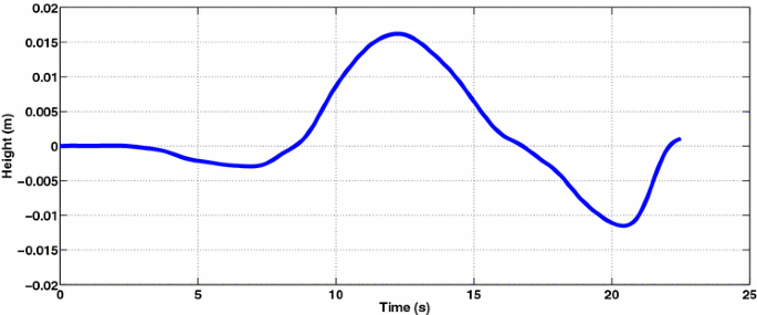

  

  Prescribed input wave for the left boundary condition, defined from t = 0 to t = 22.5 s

• Initial condition: water at rest.

• Grid resolution: a 393 × 244-size mesh was used, with the same resolution (0.014 m) as the bathymetry. Table 10 collects grid information.

  Table 10 Mesh information showing grid resolution, number of cells and computing time needed for a 200-s simulation

• Time stepping: variable time stepping based on a CFL condition.

• CFL: 0.9

• Versions of the code: Tsunami-HySEA second order with MUSCL reconstruction and WAF models used for this benchmark. Second-order model results are presented.

3.4.2 Tasks to be Performed

To accomplish this benchmark, the following tasks had to be performed:

• 1. Model the propagation of the incident and reflective wave according to the benchmark-specified boundary condition.

• 2. Compare the numerical and laboratory-measured water level dynamics at gauges 5, 7, and 9 (in Fig. 24).

• 3. Show snapshots of the numerically computed water level at time synchronous with those of the video frames; it is recommended that each modeler finds times of the snapshots that best fit the data.

• 4. Compute maximum runup in the narrow valley.

3.4.3 Numerical Result

In this section, we present the numerical results for BP7 as simulated by Tsunami-HySEA according to the tasks to be performed as given in the benchmark description.

3.4.3.1 Gauge Comparison

Figure 26 shows a comparison of Tsunami-HySEA results with the laboratory values for the three requested gauges from t = 0 to t = 30 s. Superimposed is the normalized root mean square deviation (NRMSD). A mean value of 7.66% for the NRMSD is obtained for all the three gauges for the time series simulating the first 30 s.

Fig. 26

Comparison experimental and simulated water level at gauges 5, 7, and 9 from t = 0 to t = 30 s

3.4.3.2 Frame Comparisons

In the laboratory experiment, the evolution of the wave was recorded. Five frames (Frames 10, 25, 40, 55, and 70) extracted from the video record of the lab experiment with 0.5-s interval are shown in the left column of Fig. 27. These frames focus on the narrow gully where the highest runup is observed. On the right-hand side of Fig. 27, snapshots of the numerically computed water level at times t = 15, 15.5, 16, 16.5, and 17 in seconds are presented for comparison. A good agreement of the numerical solution to observations in time and space is revealed, and it can be observed how the numerical model is able to capture the rapid runup/rundown sequence in this particular key location.

Fig. 27

Comparison of snapshots of the laboratory experiment with the numerical simulation. a Frame 10—time 15 s, b frame 25—time 15.5 s, c frame 40—time 16 s, d frame 55—time 16.5 s, e frame 70—time 17 s

3.4.3.3 Runup in the Valley

A maximum simulated runup height of 0.0891 (compared with the 0.08958 experimentally measured) is reached at time t = 16.3 s at point (5.1559, 1.8896). Figure 28 shows the frame corresponding to time t = 16.3 s, where the computed maximum runup location is marked with a red dot.

Fig. 28

Maximum simulated runup, reached at time t = 16.3 s, at point (5.15592, 1.88961), reaching a maximum height of 0.0891 (versus the 0.08958 experimentally measured)

3.5 Benchmark Problem #9: Okushiri Island Tsunami—Field

The goal of this benchmark problem is to compare computed model results with field measurements gathered after the 12 July 1993 Hokkaido Nansei-Oki tsunami (also commonly referred to as the Okushiri tsunami).

3.5.1 Problem setup

The main items describing the setup of the numerical problem are:

• Friction: Manning coefficient 0.03.

• Boundary conditions: non-reflective boundary conditions at open sea, at coastal areas inundation is computed.

• Computational domain: a nested mesh technique is used with four levels (i.e., the global mesh with three levels of refinement, see Figs. 29 and 30).

  Fig. 29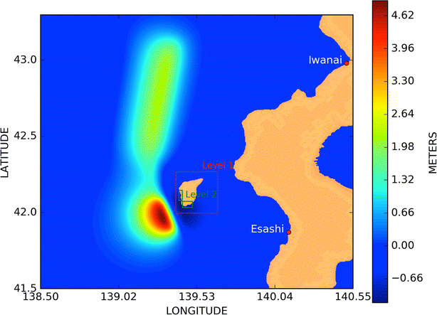

  

  Computational domain considered (level 0) showing the initial condition for Benchmark problem #9. Nested meshes level 1 and level 2 (the latter composed of two submeshes) are also depicted

  Fig. 30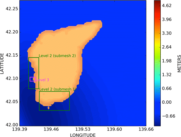

  

  Level 1 nested mesh computational domain containing the two level 2 submeshes, the region to the South including Aonae and Hamatsumae areas and the coastal region to the West containing Monai area, refined with one level 3 nested mesh around Monai Valley

  • Global mesh coverage in lon/lat [138.504, 140.552] × [41.5017, 43.2984].

    • Number of cells: 1152 × 1011 = 1,164,672.

    • Resolution: 6.4 arc-sec (≈192 m).

  • Level 1. Spatial coverage [139.39, 139.664] × [41.9963, 42.2702].

    • Refinement ratio: 4.

    • Number of cells: 616 × 616 = 379,456.

    • Resolution: 1.6 arc-sec (≈40 m).

  • Level 2. Refinement ratio: 4. Resolution: 0.4 arc-sec (≈12 m).

    • Submesh 1: large area around Monai.

      • Spatial coverage [139.434, 139,499] × [42.0315, 42.0724].

      • Number of cells: 584 × 368 = 214,912.

    • Submesh 2: Aonae cape and Hamatsumae region.

      • Spatial coverage [139.411, 139.433] × [42.0782, 42.1455].

      • Number of cells: 196 × 604 = 118,384.

  • Level 3 (Monai region). Spatial coverage [139.414, 139.426] × [42.0947, 42.1033].

    • Refinement ratio: 16.

    • Number of cells: 1744 × 1248 = 2,216,448.

    • Resolution: 0.025 arc-sec (≈0.75 m).

• Initial condition: generated by DCRC (Disaster Control Research Center), Japan. Hipocenter depth 37 km at 139.32°E and 42.76°N, M _w 7.8 (Takahashi 1996) (Fig. 29, source model DCRC 17a).

• Topobatymetric data: Kansai University.

• CFL: 0.9.

• Version of the code: Tsunami-HySEA WAF.

3.5.2 Tasks to be Performed

To evaluate performance requirements for this benchmark, the following tasks had to be performed:

• 1. Compute runup around Aonae.

• 2. Compute arrival of the first wave to Aonae.

• 3. Show two waves at Aonae approximately 10 min apart; the first wave came from the west, the second wave came from the east.

• 4. Compute water level at Iwanai and Esashi tide gauges.

• 5. Maximum modeled runup distribution around Okushiri Island.

• 6. Modeled runup height at Hamatsumae.

• 7. Modeled runup height at a valley north of Monai.

3.5.3 Numerical Results

In this section, the numerical results obtained with Tsunami-HySEA for BP9 are presented.

3.5.3.1 Runup Around Aonae

Figure 31 shows the inundation level around Aonae peninsula. The figure includes 4-m contours of bathymetry and topography. The contours allow to determine that the maximum runup height is below 12 m in the eastern part of the peninsula where the tsunami inundation is mainly produced by the second wave and where the topography is flatter producing, despite the lower runup, a further penetration. The opposite situation occurs in the western part of the peninsula: a higher runup ranging from 16 to 20 m, within a narrower strip, mainly flooded by the first wave arriving from the west. The southern part of the peninsula is inundated with a runup height of 16 meters and a large inundated area, suffering both impacts of the western and eastern tsunami wave.

Fig. 31

Inundation map of the Aonae Peninsula. This is for t < 12.59 min. The color map shows the maximum fluid depth over entire computation. 4-m contours of bathymetry and topography are shown

3.5.3.2 First Wave to Aoane

Figure 32 shows the arrival of the first wave, coming from the west, to the Aonae peninsula at times t = 4.75 min and t = 5 min. From this figure, we can conclude the time of arrival of this first wave to Aoane takes place at approximately t = 5 min. Within 15 s the wave is close to reaching the western coastline of the peninsula and at t = 5 min it has already impacted, from north to south, along all the western seashore.

Fig. 32

Zoom on the Aonae Peninsula showing the arrival of the first wave coming from the west at times t = 4.75 min and t = 5 min. We observe that this first wave impacts the west coast of the Aonae Peninsula at time close to 5 min after the tsunami generation

3.5.3.3 Waves Arriving to Aonae

Figure 33 depicts two snapshots of the arrival of two tsunami waves at the Aonae peninsula. The first wave arrival, from the west, is seen at about t = 5 min, as is shown in Fig. 32. The second major wave arrives from the east at about 9.5 min. Snapshots at time t = 5.25 min and t = 9.75 min are presented in Fig. 33.

Fig. 33

Zoom on the Aonae peninsula showing the first wave arriving from the west at time t = 5.25 min and the second wave coming from the east at time t = 9.75 min

3.5.3.4 Tide gauges at Iwanai and Esashi

Figure 34 shows the comparison between the computed and observed water levels at two tide stations located along the west coast of Hokkaido Island, Iwanai and Esashi. Besides, the maximum error in the maximum wave amplitude and the normalized root mean square deviation (NRMSD) is depicted for both time series. The errors in the maximum amplitude, although high (36 and 41%) are analogous to the mean of the models collected in NTHMP (2012) report (36 and 43%, respectively). No values were given for the NRMSD there.

Fig. 34

Computed and observed water levels at two tide stations located along the west coast of Hokkaido Island, Iwanai in upper panel and Esashi in lower panel. Observations from Yeh et al. (1996)

3.5.3.5 Maximum Runup Around Okushiri

Figure 35 shows a bar plot that compares model runup at 19 regions around Okushiri Island with measured data. In the NTHMP-provided script, runup error is evaluated by a comparison between computed and measured sets of minimal, maximal, and mean runup values in unspecified surroundings of prescribed reference points. We have searched for the set of observations used for each region to compute the minimal, maximal, and mean values (these are the three values required for generating Fig. 35). For each of these observed values the closer or the two closer model values were considered for the computation of the minimum, maximum, and the average in the given region. When only one measured data were available in a region, then the three closer model discretized points were taken (this means a larger spread in simulated values than in measured data that can be observed in regions 3, 4,5, 7, 15, and 17). This procedure was used in all cases, but in the regions with refined meshes (regions 6, 9, 10, and 11), where all computed values were used.

Fig. 35

Computed and observed runup in meters at 19 regions along the coast of Okushiri Island after 1993 Okushiri tsunami. Observations from Kato and Tsuji (1994)

In Table 11 the location of the points identifying these 19 regions are gathered and for each region the number of observations used to determine minimal, maximal, and mean values are given in column #OBS. Finally, this table also presents Tsunami-HySEA runup error at each location compared with the mean of models in NTHMP (2012). The main question that arises when regarding this table is why there are locations with such a good agreement with observed data and for other regions the agreement is so poor. First of all, we are dealing with discrete observed values taken at locations that we do not know why or how were chosen. This is a first source of uncertainty. Second, bathymetry data resolution is very inhomogeneous: where bathymetry data are finer, closer model vs observed data comparisons are obtained. Large errors are associated with low bathymetry data resolution regions. Finally, numerical resolution also varies, and besides it is finer in regions with higher resolution bathymetry data and coarser in regions with low-resolution bathymetry. Besides, as pointed out in NTHMP (2012), the accuracy of the seismic source being used and the accuracy in some of the field observations and tide gauges may also play an important role to explain the observed discrepancies. A detailed study trying to clarify these aspects is needed.

Table 11 Tsunami-HySEA model relative error with respect to field measurement data for runup around Okushiri Island. Comparison with average error values for models in NTHMP (2102). #OBS gives the number of observations used to compute the error bars in Fig. 37

3.5.3.6 Runup Height at Hamatsumae

Figure 36 shows the maximum inundation on the Hamatsumae region computed for [0, 14] min. The color map shows the maximum fluid depth along the entire simulation. The figure also depicts 4-m contours of bathymetry and topography. Maximum runups are between 8 and 16 meters, with increasing values from west to east.

Fig. 36

Inundation map of the Hamatsumae neighborhood. For t < 14 min. The color map shows the maximum fluid depth along the entire simulation. 4-m contours of bathymetry and topography are shown

3.5.3.7 Runup Height at a Valley North of Monai

Figure 37 shows the maximum inundation at a valley north of Monai, computed for [0, 4.5] min. The color map shows the maximum fluid depth along the entire simulation. The 4-m contours of topography allow to determine maximum runups that range between 8 and 12 m to the south, around 16 to the north and up to the 31.753 m of maximum computed runup, very close to the observed value, 31.7 m.

Fig. 37

Inundation map of the valley north of Monai. 4-m contours of bathymetry and topography are shown

4 Conclusions

The Tsunami-HySEA numerical model is validated and verified using NOAA standards and criteria for inundation. The numerical solutions are tested against analytical predictions (BP1, solitary wave on a simple beach), laboratory measurements (BP4, solitary wave on a simple beach; BP6, solitary wave on a conical island; and BP7, runup on Monai Valley beach), and against field observations (BP9, Okushiri island tsunami). In the numerical experiments modeling the propagation and runup of a solitary wave on a canonical beach, numerical results are clearly below the established errors by the NTHMP in their 2011 report. For BP1, the mean errors measured are below 1% in all cases. In the case of BP4, several conclusions can be extracted. For the non-breaking case with H = 0.0185 the non-dispersive model produces accurate wave forms with NRMSD errors, in most cases, very close to the dispersive model results. For the breaking wave case with H = 0.30 it can be observed that the shape of the (dispersive) wave cannot be well captured by the non-dispersive model, producing large NRMSD errors at the times when the NLSW model tends to produce a shock. Nevertheless, the agreement is still high for times when non-steep profiles are present. Despite this (a dispersive model is absolutely necessary if we want to accurately reproduce the time evolution of the wave in the breaking case) we have observed that measured runup is accurately reproduced by both models in the two studied cases. On the other hand, the dispersive version of Tsunami-HySEA produces very good results in both the breaking and non-breaking cases. For BP6, dealing with the impact of a solitary wave on a conical island, again non-dispersive and dispersive Tsunami-HySEA models have been used. Wave splitting and colliding are clearly observed. Numerical results are very similar for Case A (A/h = 0.045) and Case B (A/h = 0.096) for wave shape. Larger differences are evident in Case C (A/h = 0.181), where dispersive model performs better for wave shape, but not for the computed runup. It is noteworthy that the computed maximum runups for Cases A and C are very close for both models but they clearly differ for Case B. Tsunami-HySEA model figures have been compared with figures in NTHMP (2012), performing in general better than the mean when comparing by class of model (dispersive and non-dispersive). BP7, the laboratory experiment dealing with the tsunami runup onto a complex 3D model of the Monai Valley beach, was studied in detail in (Gallardo et al. 2007). A mean value of 7.66% for the NRMSD is obtained for all the three gauges for the times series simulating the first 30 s. The snapshots of the simulation agree well with the experimental frames and, finally, a maximum simulated runup height of 0.0891 is obtained compared with the 0.08958 experimentally measured. Comparison of BP9 with Okushiri island tsunami observed data is performed using nested meshes with two level 2 meshes located one in the South of the island, covering Aoane and Hamatsumae areas and the second one to the West containing Monai area. Finally, one level 3 refined mesh is located covering the Monai area. Computed runup and arrival times are in good agreement with observations. Water level time series at Iwanai and Esashi tide gauges show large NRMSD and large errors in the maximum amplitude (36 and 41% for ERR) but analogous to the mean of the models in NTHMP (2012) (36 and 43% for ERR). For the maximum runup at 19 regions around Okushiri Island a mean error of 15% is obtained, the same as the mean of models in NTHMP (2012), with 10 regions with errors below 10%. Regions located in areas with refined meshes perform much better than regions located in coarse mesh areas.

References

Apotsos, A., Buckley, M., Gelfenbaum, G., Jafe, B., & Vatvani, D. (2011). Pure and Applied Geophysics, 168(11), 2097–2119. doi:10.1007/s00024-011-0291-5.
Briggs, M., Synolakis, C., Harkins, G., & Green, D. (1995). Laboratory experiments of tsunami runup in a circular island. Pure and Applied Geophysics, 144, 569–593.
Castro, M.J., de la Asunción, M., Macías, J., Parés, C., Fernández-Nieto, E.D., González-Vida, J.M., Morales, T. (2012). IFCP Riemann solver: Application to tsunami modelling using GPUs. In E. Vázquez, A. Hidalgo, P. García, L. Cea eds. CRC Press. Chapter 5, 237–244.
Castro, M. J., & Fernández-Nieto, E. D. (2012). A class of computationally fast first order finite volume solvers: PVM methods. SIAM Journal on Scientific Computing, 34, A2173–A2196.
Castro, M. J., Fernández-Nieto, E. D., Ferreiro, A. M., García-Rodríguez, J. A., & Parés, C. (2009). High order extensions of Roe schemes for two-dimensional non-conservative hyperbolic systems. Journal of Scientific Computing, 39(1), 67–114.
Castro, M. J., Ferreiro, A., García, J. A., González, J. M., Macías, J., Parés, C., et al. (2005). On the numerical treatment of wet/dry fronts in shallow flows: applications to one-layer and two-layer systems. Mathematical and Computer Modelling, 42(3–4), 419–439.
Castro, M. J., González, J. M., & Parés, C. (2006). Numerical treatment of wet/dry fronts in shallow flows with a modified Roe scheme. Mathematical Models and Methods in Applied Sciences, 16(6), 897–931.
Castro, M. J., Ortega, S., Asunción, M., Mantas, J. M., & Gallardo, J. M. (2011). GPU computing for shallow water flow simulation based on finite volume schemes. Comptes Rendus Mécanique, 339, 165–184.
de la Asunción, M., Castro, M. J., Fernández-Nieto, E. D., Mantas, J. M., Ortega, S., & González-Vida, J. M. (2013). Efficient GPU implementation of a two waves TVD-WAF method for the two-dimensional one layer shallow water system on structured meshes. Computers & Fluids, 80, 441–452.
de la Asunción, M., Mantas, J. M., & Castro, M. J. (2011). Simulation of one-layer shallow water systems on multicore and CUDA architectures. The Journal of Supercomputing, 58, 206–214.
Gallardo, J. M., Ortega, S., de la Asunción, M., & Mantas, J. M. (2011). Two-dimensional compact third-order polynomial reconstructions. Solving non-conservative hyperbolic systems using GPUs. Journal of Scientific Computing, 48, 141–163.
Gallardo, J. M., Parés, C., & Castro, M. J. (2007). On a well-balanced high-order finite volume scheme for shallow water equations with topography and dry areas. Journal of Computational Physics, 227, 574–601.
Gottlieb, S., & Shu, C. W. (1998). Total variation diminishing Runge-Kutta schemes. Mathematics of Computation, 67, 73–85.
Horrillo, J., Grilli, S. T., Nicolsky, D., Roeber, V., & Zhang, J. (2015). Performance benchmarking Tsunami models for nthmp’s inundation mapping activities. Pure and Applied Geophysics, 172(3), 869–884. doi:10.1007/s00024-014-0891-y.
Kato, H., & Tsuji, Y. (1994). Estimation of fault parameters of the 1993 Hokkaido-Nansei-Oki earthquake and tsunami characteristics. Bulletin of the Earthquake Research Institute, 69, 39–66.
Liu, P.L.-F., Yeh, H., & Synolakis, C. (2008). Advanced numerical models for simulating Tsunami waves and runup. Advances in coastal and ocean engineering (vol. 10). New Jersey: World Scientific.
Macías, J., Castro, M.J., González-Vida, J.M., de la Asunción, M., and Ortega, S. (2014). HySEA: An operational GPU-based model for Tsunami Early Warning Systems. EGU 2014.
Macías, J., Castro, M.J., González-Vida, and J.M., Ortega, S. (2013). Non-linear Shallow Water Models for coastal run-up simulations. EGU 2013.
Macías, J., Castro, M.J., González-Vida, J.M., Ortega, S., and de la Asunción, M. (2013). HySEA tsunami GPU-based model. Application to FTRT simulations. International Tsunami Symposium (ITS2013). Göcek (Turkey). 25–28 September 2013.
Macías, J., Castro, M.J., Ortega, S., Escalante, C., and González-Vida, J.M. (2016). Tsunami-HySEA Benchmark results. In NTHMP report for the MMS Benchmarking Workshop: Tsunami Currents.
Macías, J., Mercado, A., González-Vida, J.M., Ortega, S., and Castro, M.J. (2015). Comparison and numerical performance of Tsunami-HySEA and MOST models for LANTEX 2013 scenario. Impact assessment on Puerto Rico coasts. Pure and Applied Geophysics. doi:10.1007/s00024-016-1387-8.
Marquina, A. (1994). Local piecewise hyperbolic reconstructions for nonlinear scalar conservation laws. SIAM Journal of Scientific Computing, 15, 892–915.
National Tsunami Hazard Mitigation Program (NTHMP). 2012. Proceedings and Results of the 2011 NTHMP Model Benchmarking Workshop. Boulder: U.S. Department of Commerce/NOAA/NTHMP; NOAA Special Report. p. 436.
National Tsunami Hazard Mitigation Program (NTHMP). 2016. Report on the 2015 NTHMP Current Modeling Workshop. Portland, Oregon. p. 202.
Nicolsky, D. J., Suleimani, E. N., & Hansen, R. A. (2011). Validation and verification of a numerical model for Tsunami propagation and runup. Pure and Applied Geophysics, 168(6), 1199–1222.
Parés, C. (2006). Numerical methods for nonconservative hyperbolic systems: a theoretical framework. SIAM Journal on Numerical Analysis, 44(1), 300–321.
Roeber, V., Cheung, K. F., & Kobayashi, M. H. (2010). Shock-capturing Boussinesq-type model for nearshore wave processes. Coastal Engineering, 57, 407–423.
Synolakis, C. E. (1987). The runup of long waves. Journal of Fluid Mechanics, 185, 523–545.
Synolakis, C. E., Bernard, E. N., Titov, V. V., Kânoğlu, U., & González, F. I. (2008). Validation and verification of tsunami numerical models. Pure and Applied Geophysics, 165(11–12), 2197–2228.
Takahashi, T., 1996. Benchmark Problem 4. The 1993 Okushiri tsunami. Data, Conditions and Phenomena. In: H. Yeh, P. Liu, C. Synolakis (eds.): Long wave runup models. Singapore: World Scientific Publishing Co. Pte. Ltd., pp. 384–403.
Tolkova, E. (2014). Land-water boundary treatment for a tsunami model with dimensional splitting. Pure and Applied Geophysics, 171(9), 2289–2314.
van Leer, B. (1979). Towards the Ultimate Conservative Difference Scheme, V. A Second Order Sequel to Godunov’s Method. Journal of Computational Physics, 32, 101–136.
Yamazaki, Y., Kowalik, Z., & Cheung, K. F. (2009). Depth-integrated, non-hydrostatic model for wave breaking and run-up. International Journal for Numerical Methods in Fluids, 61(5), 473–497.
Yeh, H., Liu, P., Synolakis, C., editors (1996). Benchmark problem 4. The 1993 Okushiri Data, Conditions and Phenomena. Singapore: World Scientific Publishing Co. Pte. Ltd.
Acknowledgements
This research has been partially supported by the Spanish Government Research project SIMURISK (MTM2015-70490-C2-1-R), the Junta de Andalucía research project TESELA (P11-RNM7069), and Universidad de Málaga, Campus de Excelencia Internacional Andalucía Tech. The GPU and multi-GPU computations were performed at the Unit of Numerical Methods (UNM) of the Research Support Central Services (SCAI) of the University of Malaga.
Author information
Authors and Affiliations
Corresponding author
Rights and permissions
Open Access This article is distributed under the terms of the Creative Commons Attribution 4.0 International License (http://creativecommons.org/licenses/by/4.0/), which permits unrestricted use, distribution, and reproduction in any medium, provided you give appropriate credit to the original author(s) and the source, provide a link to the Creative Commons license, and indicate if changes were made.
About this article
Cite this article
Macías, J., Castro, M.J., Ortega, S. et al. Performance Benchmarking of Tsunami-HySEA Model for NTHMP’s Inundation Mapping Activities. Pure Appl. Geophys. 174, 3147–3183 (2017). https://doi.org/10.1007/s00024-017-1583-1
Received:
Revised:
Accepted:
Published:
Issue Date:
DOI: https://doi.org/10.1007/s00024-017-1583-1