n-Laplacians on Metric Graphs and Almost Periodic Functions: I

Abstract

The spectra of n-Laplacian operators $(-\Delta )^n$ on finite metric graphs are studied. An effective secular equation is derived and the spectral asymptotics are analysed, exploiting the fact that the secular function is close to a trigonometric polynomial. The notion of the quasispectrum is introduced, and its uniqueness is proved using the theory of almost periodic functions. To achieve this, new results concerning roots of functions close to almost periodic functions are proved. The results obtained on almost periodic functions are of general interest outside the theory of differential operators.

1 Introduction

1.1 Motivation

Quantum graphs have proved to be an important area of research in both physics and mathematics. By quantum graphs, one understands ordinary differential equations on metric graphs, coupled by matching conditions at the vertices. Most works on the subject consider second-order (Schrödinger) differential operators (see, for example, [8, 20, 21, 25, 28, 34, 36, 40, 41, 45, 51]), but the methods developed can be generalised to differential expressions of arbitrary order. This has already been done in the case of first-order (Dirac and momentum) and to some extent fourth-order operators (e.g. [11, 13, 22, 27, 32]). The recent status of research in this area is well reflected in the monographs [8, 41].

Recent development in spectral theory of Schrödinger operators on metric graphs has seen a connection with trigonometric polynomials and the classical theory of almost periodic functions (see [12, 47]). These studies were based on the Gutkin–Kottos–Smilansky formula for the secular equation for the Laplacian [28, 35]

$$\begin{aligned} \det \left[ {\mathbf {S}}_\text {e} (k){\mathbf {S}}_\text {v} (k) - {\mathbf {I}} \right] = 0 , \end{aligned}$$

(1.1)

where ${\mathbf {S}}_\text {e}$ and ${\mathbf {S}}_\text {v}$ are the edge and vertex scattering matrices (see Sect. 5), respectively. For scaling-invariant vertex conditions, ${\mathbf {S}}_\text {v}$ is independent of the energy, whilst the entries of ${\mathbf {S}}_\text {e}$ are given by exponentials with real frequencies; hence, the secular function is a trigonometric polynomial of the form

$$\begin{aligned} p(k) = \sum _{j \in J} a_j \mathrm{e}^{i r_j k}, \end{aligned}$$

(1.2)

where $a_j \in {\mathbb {C}}$ and $r_j \in {\mathbb {R}}$, not necessarily rationally dependent. For general vertex conditions and Schrödinger operators with nonzero potentials, the eigenvalues are not given by zeros of trigonometric polynomials, but are asymptotically close to such zeros, leading to the notion of asymptotic isospectrality. The approximating trigonometric polynomials correspond to Laplacians with uniquely determined scaling-invariant vertex conditions. Due to the rigidity of zeros of trigonometric polynomials, one may not only describe spectral asymptotics, but also solve certain inverse problems.

The present paper is devoted to the spectral theory of higher-order differential operators on metric graphs, more precisely of n-Laplacians associated with the differential expression $\left( - \frac{\mathrm{d}^2}{\mathrm{d}x^2} \right) ^n$ on the edges. Our goal is twofold:

• to derive an efficient parameterisation of all self-adjoint vertex conditions leading to an explicit secular equation generalising (1.1);

• to study spectral asymptotics for n-Laplacians with scaling-invariant conditions,

postponing the analysis of general vertex conditions to the second part of our study.

It appears that even the spectra of n-Laplacians with scaling-invariant vertex conditions are hardly ever described by trigonometric polynomials or, even more generally, almost periodic functions. Nevertheless, we show that such functions do play an important role in their spectral analysis. In particular we introduce the notion of the quasispectrum, which not only asymptotically approximates the actual spectrum but is also unique. The quasispectrum coincides with the (2nth root of the) spectrum of a certain Dirac operator on the same metric graph which itself is therefore described by zeros of a trigonometric polynomial. This is akin to determining the Laplacian spectrum from the eigenvalues of the Schrödinger operator in earlier works. This once again illustrates the power of almost periodic functions and the rigidity of their zeros.

A key ingredient in all of this is the study of roots of a certain class of functions which are close to almost periodic functions, holomorphic perturbations as we call them: we show that the roots of a holomorphic perturbation of an almost periodic function are aymptotically close to those of the almost periodic function. One can prove a kind of equivalence relation between such functions, which has the consequence that two n-Laplacians are asymptotically isospectral if and only if they have the same quasispectrum. For this purpose, new results concerning (classical) almost periodic functions are proved; we believe that these results have wider applications.

To understand why it is unavoidable to use almost periodic functions, as opposed to more conventional approaches, we recall the asympotics for the Schrödinger operator. The eigenvalues (discrete and accumulating towards $+ \infty$) satisfy Weyl’s law [8, 41]

$$\begin{aligned} \lambda _j = k_j^2 \sim \Big ( \frac{\pi }{{\mathcal {L}}} \Big )^2 j^2, \end{aligned}$$

with ${\mathcal {L}}$ being the total length of the graph. However, no further refinement of the asymptotics of the form $k_j = \frac{\pi }{{\mathcal {L}}} j + c_0 + c_{-1} j^{-1} + \cdots$ is possible unless the graph is an interval or a loop. One may derive certain asymptotic expansions of this type, but just for subsequences of eigenvalues like in [16].

In the first half of this paper, we revise the issue of vertex conditions. There is already a well-established theory for parameterising self-adjoint extensions of symmetric operators by unitary matrices using boundary triples (see [14, 18, 19, 26, 33]). Equivalent, more classical approaches include von Neumann extension theory (see [56]) or Birman–Krein–Vishik theory (see [1]). For Schrödinger operators on metric graphs, parameterisation of vertex conditions via the scattering matrix has proved to be useful, not least due to clear physical interpretation of the parameter. Our first goal was thus to establish a similar approach for n-Laplacians. Using unitary parameterisation via boundary triples, one can easily describe which conditions are scaling-invariant, or non-Robin, but the corresponding secular equation is difficult to analyse. Therefore, we develop an alternative approach via the so-called vertex transmission matrix which leads to a more effective secular equation, allowing one to study spectral asymptotics. Note that in the case of the Laplacian ($n=1$), the two approaches are identical, and the parameter coincides with the vertex scattering matrix. Surprisingly the secular equation for higher-order operators has not been written in any form yet.

In the second half of the paper, the focus turns to almost periodic functions, and from this, we establish spectral asymptotics for n-Laplacians with scaling-invariant vertex conditions by comparing the secular equation with a certain reference trigonometric polynomial, the set of whose positive roots we identify as the quasispectum. As we have already mentioned, the quasispectrum is unique and can be interpreted as the spectrum of a Dirac operator. This operator replaces the reference Laplacian (denoted $L_0^{{\mathbf {S}}_{\mathrm{v}} (\infty )}$ in [47]) used to describe the asymptotics for the Schrödinger equation.

Throughout this paper, we are focused on the 2nth derivative $(-\Delta )^n$, but the results obtained open the way to studying spectral asymptotics for arbitrary ordinary differential operators on graphs with the most general vertex conditions and variable coefficients.

1.2 Vertex Conditions and Spectral Asymptotics

From a mathematical point of view, quantum graphs is a perfect area for experiment relating to extension theory of symmetric operators. The most general vertex conditions for self-adjoint extensions of symmetric operators can be described using the theory of boundary triples [6], also [26, 33]. For Laplacians on metric graphs, all possible vertex conditions were first described in [34]; this approach resembles our formula (2.5) and has the disadvantage of being non-unique—multiplying all matrices $A_r$ by an invertible matrix does not change the linear solution subspace. Two alternative but complementing approaches leading to unique set of parameters were suggested in [36] (in terms of a linear subspace and a Hermitian matrix) and [45] (in terms of the vertex scattering matrix). The first approach is efficient when working with the quadratic form and therefore is efficient in proving spectral estimates, whilst the vertex scattering matrix used in the second approach directly appears in the secular equation. Methods for estimating eigenvalues, such as graph surgery, are discussed in [7, 23, 30, 31, 42, 43, 52], and properties of the ground state in the presence of a potential in [39, 46]. Spectral asymptotics are discussed in [16, 37, 47, 48]. The notion of isospectrality for these operators was first discussed in [28] and then in [4, 5, 53], and asymptotic isospectrality in [47]. Inverse problems are addressed in [2, 3, 38, 43, 48, 54, 55].

In the case of bi-Laplacians, a characterisation of all vertex conditions corresponding to self-adjoint operators can be found in [27]. More detailed expositions involving spectra (e.g. Weyl asymptotics) for bi-Laplacians with selected vertex conditions can be found for instance in [17]. See also [49] for physical and [32] for mathematical interpretations of certain conditions. Vertex conditions for differential operators of arbitrary order have been derived in [15]; the parameterisation again resembles our formula (2.5).

2 Differential Operators on Metric Graphs

Matrices of various sizes in terms of the natural numbers d and n, recurring throughout this paper, will play a range of roles. The most important matrices have sizes $d\times d$, which for consistency we denote in bold, e.g. ${\mathbf {A}}$, and $nd\times nd$, which are double-struck, e.g. ${\mathbb {A}}$. Those of other sizes have no special notation, e.g. A, and in that case the dimensions are always specified.

2.1 Differential Operators: Metric Graphs and Vertex Conditions

Let E be a finite set of edges, that is, intervals taken from different copies of ${\mathbb {R}}$. Let $N:=|E|$ be the total number of edges, and d the total number of endpoints. For the majority of this paper, we consider only compact graphs, so the intervals are all bounded, in which case $d=2N$. Labelling the edges in E as $e_1,\dots e_N$, we shall label the endpoints $x_1,\dots ,x_d$ to satisfy $e_j=[x_j,x_{N+j}]$ for $j=1,\dots ,N$.¹ Under this labelling, if $j\le N$ then we call $x_j$ (the smallest value in the interval) a left endpoint, whilst for $N<j\le d$, we call $x_j$ (the largest value in the interval) a right endpoint. Where necessary, we denote by $e(x_j)$ the edge that has $x_j$ as an endpoint.

Consider the set of all endpoints $\left\{ x_j \right\} _{j=1}^d$ and its partition into M equivalence classes v forming the vertex set V:

$$\begin{aligned} \begin{array}{l} \displaystyle v' \cap v'' = \emptyset , \quad v' \ne v'', \\ \displaystyle \bigcup _{v \in V} v = \left\{ x_j \right\} _{j=1}^{2N}. \end{array} \end{aligned}$$

The set of vertices induces an equivalence relation $\sim$ on the disjoint union of edges as follows: given $x,y\in \bigsqcup _{e\in E}e$, we say that $x\sim y$ if and only if either

• (i) x and y belong to the same edge $e\in E$ and $x=y$, or

• (ii) x and y are endpoints that belong to the same vertex v.

This equivalence relation yields a metric graph

$$\begin{aligned} \Gamma :=\bigsqcup _{e\in E}e\Bigg /\sim . \end{aligned}$$

(2.1)

Given a metric graph $\Gamma$, we are interested in operators in the Hilbert space $L_2(\Gamma ):=\bigoplus _{e\in E} L_2(e)$. The inner product associated with this space is the sum of standard $L_2$ inner products on each edge $e\in E$. Explicitly, that is

$$\begin{aligned} \langle \phi ,\psi \rangle =\langle \phi ,\psi \rangle _{L_2(\Gamma )}:=\sum _{e\in E}\int _e\overline{\phi (x)}\psi (x)\,\mathrm {d}x,\qquad \phi ,\psi \in L_2(\Gamma ). \end{aligned}$$

(2.2)

We usually omit the subscript when writing the $L_2(\Gamma )$ inner product.

The focus of this paper is on differential operators in $L_2(\Gamma )$ with formal expression ${\mathfrak {p}}^{2n}$ for some $n\in {\mathbb {N}}$, where ${\mathfrak {p}}:=-\mathrm {i}\frac{\mathrm {d}}{\mathrm {d}x}$. However, for later convenience, the following conventions are stated more generally permitting $n\in \frac{1}{2}{\mathbb {N}}$. The functions in the domain of such an operator are all from the Sobolev space ${{\widetilde{H}}}^{2n}(\Gamma )$, which is the set of functions in $L_2(\Gamma )$ which on each edge e are contained in the Sobolev space $H^{2n}(e)=W_2^{2n}(e)$. In general, we shall impose further restrictions on the domain in the form of linear conditions at the endpoints. To be able to write such conditions independently of the direction of parameterisation of the edges, we define for each $r=0,1,...,2n-1$ the normal r th derivative of $\psi \in {{\widetilde{H}}}^{2n}(\Gamma )$ at the endpoint $x_j$ to be

$$\begin{aligned} \partial ^r\psi (x_j):=\sigma (x_j)^r\lim _{x\rightarrow x_j}\frac{\mathrm {d}^r}{\mathrm {d}x^r}\psi (x), \end{aligned}$$

(2.3)

where

$$\begin{aligned} \sigma (x_j):= {\left\{ \begin{array}{ll} +1&{}\quad \text {if }x_j\text { is a left endpoint,}\\ -1&{}\quad \text {if }x_j\text { is a right endpoint.}\end{array}\right. } \end{aligned}$$

(2.4)

We then denote by $\partial ^r\varvec{\Psi }$ the vector of normal rth derivatives at all endpoints of E (ordered according to the indices of the endpoints). We usually write $\varvec{\Psi }:=\partial ^0\varvec{\Psi }$.

Given $n\in \frac{1}{2}{\mathbb {N}}$, the most general (linear) boundary conditions that can be imposed on functions in ${{\widetilde{H}}}^{2n}(\Gamma )$ are of the form

$$\begin{aligned} \sum _{r=0}^{2n-1} A_r\partial ^r\varvec{\Psi }=0, \end{aligned}$$

(2.5)

where $A_0, A_1,\dots , A_{2n-1}$ are arbitrary $l\times d$ matrices for a certain $l\in {\mathbb {N}}$. Without loss of generality, it may be assumed that $l\le 2nd$ since otherwise there will certainly be redundancies. Taking $l=2nd$ is thus sufficient to express all possible conditions using matrices of consistent dimensions.

The domain of an operator in $L_2(\Gamma )$ given by with boundary conditions (2.5) is

(2.6)

The conditions governed by (2.5) are called the vertex conditions for . Note that the matrices $A_r$ are not uniquely determined by the solution space for (2.5). For integer n, it will be established in Sect. 3.1 that any vertex conditions leading to self-adjoint operators can be written in this form with $l=nd$.

The Hilbert spaces $L_2(\Gamma )$ and ${{\widetilde{H}}}^{2n}(\Gamma )$ are independent of the vertex structure, i.e. how the edges are connected to one another. In other words, one could substitute $\Gamma$ with any other metric graph with the same edges, and the Hilbert spaces would be the same. However, it is natural to assume that the vertex conditions (2.5) of an operator in $L_2(\Gamma )$ respect the vertex structure of $\Gamma$. This means that the conditions can be written separately connecting boundary values associated with each vertex v. In other words, considering equivalent conditions and simultaneously permuting the endpoints from ${\mathbb {C}}^d$, all matrices $A_r$ can be put into the same block diagonal form determined by the vertices. Moreover, such representation should be minimal in the sense that it is impossible to write equivalent vertex conditions with a finer partition of the endpoints into equivalence classes.

Everything that has been said so far can clearly be adapted for more general linear differential expressions ${\mathfrak {a}}$, but one would have to be more careful when stating the admissible domains.

2.2 First-Order Operators

The first-order differential operators in $L_2(\Gamma )$ with expression ${\mathfrak {p}}$ are the only odd-ordered operators that will play a significant role in our studies (see for instance [22]). Fixing $l\ge d$, vertex conditions of any such operator with differential expression ${\mathfrak {p}}$ can be expressed in the form $A_0\varvec{\Psi }=0$ for some $l\times d$ matrix $A_0$.² Given such a matrix $A_0$, denote by $[ A_0]$ its equivalence class modulo left multiplication by invertible $l\times l$ matrices. The vertex conditions corresponding to any element of this class are equivalent. Denote by the operator with these vertex conditions. Defining the sign matrix

$$\begin{aligned} \varvec{\Sigma }:=\text {diag}(\sigma (x_1),\dots ,\sigma (x_d)), \end{aligned}$$

(2.7)

and $\sigma (x_j)$ is given by (2.4), the following simple result holds.

Lemma 2.1

The adjoint of the operator is given by

(2.8)

where $B_0$ is any $l\times d$ matrix with $rank (B_0)=d-rank ( A_0 )$ and such that $A_0B_0^*=0$.

Proof

The domain of is the set of $\phi \in L_2(\Gamma )$ for which is bounded among $\psi \in \text {dom}(A)$ with respect to the $L_2$-norm. Taking $\psi \in C_0^\infty (e)$, we see that is contained in $\bigoplus _e W_2^1 (e).$ For $\phi \in \bigoplus _e W_2^1 (e)$, the inner product equates to $\langle {\mathfrak {p}}\phi ,\psi \rangle -\mathrm {i}\langle \varvec{\Sigma }\varvec{\Phi },\varvec{\Psi }\rangle _{{\mathbb {C}}^d}$. As $\ker A_0=\text {ran}\,B_0^*$ for any matrix $B_0$ like in the statement of the lemma, this form is bounded if and only if $\langle \varvec{\Sigma }\varvec{\Phi },\varvec{\Psi }\rangle _{{\mathbb {C}}^d}=0$ for all $\varvec{\Psi }\in \text {ran}\,B_0^*$, that is if and only if $\varvec{\Sigma }\varvec{\Phi }\in \ker B_0$. $\square$

For instance, the minimal operator is related to the maximal operator via . The product is a Laplacian with Dirichlet vertex conditions at all endpoints, whilst has Neumann vertex conditions at all endpoints. The metric graphs whose vertex structure is respected by the vertex conditions of these operators have all their edges disconnected. On the other hand, given a metric graph $\Gamma$, if is the operator which imposes continuity of functions in its domain at the vertices of $\Gamma$, then is the operator which imposes the condition that $\sum _{x_j\in v}\sigma (x_j)\psi (x_j)=0$ at each vertex v. Then the domain of the Laplacian

(2.9)

consists of functions $\psi \in {{\widetilde{H}}}^{2n}(\Gamma )$ satisfying continuity and the Kirchhoff condition $\sum _{x_j\in v}\partial \psi (x_j)=0$ at every vertex v: these vertex conditions for this operator are frequently referred to in the literature as (among other names) standard vertex conditions for $\Gamma$ (see [45]). Note that representation (2.9) was used in [24], leading to interesting results.

3 n-Laplacians on Metric Graphs

An n -Laplacian on $\Gamma$ is an operator in $L_2(\Gamma )$ with differential expression $(-\Delta )^n$, where $-\Delta :={\mathfrak {p}}^2=-\frac{\mathrm {d}^2}{\mathrm {d}x^2}$ and $n\in {\mathbb {N}}$: it shall always be assumed that it has vertex conditions of the form (2.5). One may choose to assume in everything which follows that the n-Laplacians in $L_2(\Gamma )$ respect the vertex structure of $\Gamma$, except where explicitly stated otherwise. Our first task is to establish which vertex conditions lead to self-adjoint operators.

3.1 Self-Adjoint n-Laplacians

To establish which vertex conditions correspond to self-adjoint n-Laplacians, we define the minimal n -Laplacian in $L_2(\Gamma )$ to be the operator which has differential expression $(-\Delta )^n$ and domain given by

This is the symmetric n-Laplacian in $L_2(\Gamma )$ with the smallest domain characterised by imposing vertex conditions on functions in ${{\widetilde{H}}}^{2n}(\Gamma )$. We refer to its adjoint as the maximal n -Laplacian in $L_2(\Gamma )$, having the same differential expression, but with the domain . Generically, neither of these operators respect the vertex structure of $\Gamma$. Every self-adjoint n-Laplacian in $L_2(\Gamma )$ is an extension of and a restriction of . To describe all such self-adjoint operators, one may use the formalism of boundary triples.

Given a symmetric operator in a Hilbert space ${\mathfrak {H}}$, a boundary triple $({\mathcal {H}},\varvec{\Gamma }_0,\varvec{\Gamma }_1)$ for consists of a Hilbert space ${\mathcal {H}}$ called the boundary space, together with two boundary maps such that

for some real constant c. The dimension of ${\mathcal {H}}$ must be equal to the defect index of (Theorem 1.5, Ch. 3, [26]); for n-Laplacians in $L_2(\Gamma )$, this will be nd.

Proposition 3.1

(Theorem 1.6, Ch. 3, [26]). Let $({\mathcal {H}},\varvec{\Gamma }_0,\varvec{\Gamma }_1)$ be a boundary triple for an operator on a Hilbert space ${\mathfrak {H}}$. Then an extension of is self-adjoint if and only if there exists a $\dim ({\mathcal {H}})\times \dim ({\mathcal {H}})$ unitary matrix ${\mathbb {U}}$ such that is the largest subset of on which

$$\begin{aligned} \mathrm {i}({\mathbb {U}}-{\mathbb {I}})\varvec{\Gamma }_0=({\mathbb {U}} +{\mathbb {I}})\varvec{\Gamma }_1 \end{aligned}$$

holds.

The sesquilinear boundary form for the n-Laplacian is given by $\Omega (\phi ,\psi )=\langle \phi , (-\Delta )^n \psi \rangle -\langle (-\Delta )^n \phi ,\psi \rangle$ for all . To derive an explicit expression, we define for each $k\in {\mathbb {R}}\backslash \{0\}$ the boundary maps $\varvec{\Gamma }_0(k),\varvec{\Gamma }_1(k): {{\widetilde{H}}}^{2n}(\Gamma )\rightarrow {\mathbb {C}}^{nd}$ by

(3.1)

Here, ${\mathbb {C}}^{nd}$ is the boundary space. Integration by parts implies that

$$\begin{aligned} \Omega (\phi ,\psi )=-\frac{1}{k^{2n-1}}\left\{ \langle \varvec{\Gamma }_0(k) \phi ,\varvec{\Gamma }_1(k)\psi \rangle _{{\mathbb {C}}^{nd}} -\langle \varvec{\Gamma }_1(k)\phi ,\varvec{\Gamma }_0(k) \psi \rangle _{{\mathbb {C}}^{nd}}\right\} , \end{aligned}$$

(3.2)

for , independently of k. Thus, $({\mathbb {C}}^{nd},\varvec{\Gamma }_0(k),\varvec{\Gamma }_1(k))$ is a boundary triple for for any real $k \ne 0$ .

The following type of result is a standard ingredient in the theory of boundary triples. For Schrödinger operators on metric graphs, see Lemma 2.2, [34], equation (10), [29], Theorem 6, [36], and Theorem 2.6, [45]; these results are summarised in Theorem 1.4.4, [8]. Our theorem can be seen as a generalisation of these results in the Laplacian case, together with Theorem 3.1, [27] for bi-Laplacians, and Theorem 3.4, [15] for higher-order operators. Operators here are not required to respect the vertex structure of $\Gamma$.

Theorem 3.2

Let be an n-Laplacian in $L_2(\Gamma )$ with fixed vertex conditions. For any given $k\in {\mathbb {R}}\backslash \{0\}$, let $\varvec{\Gamma }_0(k),\varvec{\Gamma }_1(k): {{\widetilde{H}}}^{2n}(\Gamma )\rightarrow {\mathbb {C}}^{nd}$ be the boundary maps (3.1). Then, the following are equivalent:

• (a) is self-adjoint;

• (b) there exists an $nd\times nd$ unitary matrix ${\mathbb {U}}(k)$ such that if and only if

  $$\begin{aligned} \mathrm {i}({\mathbb {U}}(k)-{\mathbb {I}})\varvec{\Gamma }_0(k) \psi =({\mathbb {U}}(k)+{\mathbb {I}})\varvec{\Gamma }_1(k)\psi ; \end{aligned}$$

  (3.3)

• (c) there exist a subspace $X\subseteq {\mathbb {C}}^{nd}$ and a Hermitian linear map $T\in {\mathcal {L}}(X)$ such that if and only if

  $$\begin{aligned} \varvec{\Gamma }_0(1)\psi \in X,\qquad \varvec{\Gamma }_1(1) \psi +T\varvec{\Gamma }_0(1)\psi \in X^\perp ; \end{aligned}$$

  (3.4)

• (d) there exist matrices $A_0, A_1,\dots , A_{2n-1}$ of size $nd\times d$ for which

  $$\begin{aligned} \sum _{j=0}^{n-1}(-1)^j A_j A_{2n-1-j}^* \end{aligned}$$

  (3.5)

  is Hermitian and the concatenated matrix $\left( A_0\Bigg | A_1\Bigg |\ldots \Bigg | A_{2n-1}\right)$ has maximal rank nd, such that if and only if

  $$\begin{aligned} \sum _{s=0}^{2n-1} A_s\partial ^s\varvec{\Psi }=0. \end{aligned}$$

  (3.6)

Proof

See “Appendix A.” $\square$

Remark

The concatenated matrix $\left( A_0\Bigg | A_1\Bigg |\ldots \Bigg | A_{2n-1}\right)$ defining the vertex conditions (3.6) of a self-adjoint n-Laplacian is unique up to left multiplication by an invertible $nd\times nd$ matrix.

Example 3.3

A bi-Laplacian in $L_2(\Gamma )$ is self-adjoint if and only if its vertex conditions can be written in the form $A_0\varvec{\Psi }+A_1\partial \varvec{\Psi }+A_2\partial ^2\varvec{\Psi }+A_3\partial ^3\varvec{\Psi }=0$ for some $2d\times d$ matrices $A_0,A_1,A_2,A_3$ such that $A_0A_3^*-A_1A_2^*$ is Hermitian and $\text {rank}\left( A_0\Bigg |A_1\Bigg |A_2\Bigg |A_3\right) =2d$.

For any prescribed $k\in {\mathbb {R}}\backslash \{0\}$, the unitary matrix ${\mathbb {U}}(k)$ serves as a parameter for all self-adjoint n-Laplacians in $L_2(\Gamma )$. More precisely, writing to avoid ambiguity, the map gives a bijection between the set of unitary $nd\times nd$ matrices and the set of all self-adjoint n-Laplacians on graphs formed of the edges in E (not just those which respect the vertex structure). The unitary parameter can be computed explicitly using formula (A.5) in “Appendix A,” given the vertex conditions written in the form (3.6), and is a unitary matrix-valued holomorphic function of k. For Laplacians, ${\mathbb {U}}(k)$ is just the vertex scattering matrix from the existing literature (see [45]). For higher n, it serves as an analogue purely by virtue of equation (3.3), although is not itself a scattering matrix for the associated n-Laplacian in any rigorous physical or mathematical sense. The matrix which better fits that role is introduced in Sect. 4.2.

As in the Laplacian ($n=1$) case, the unitary parameter easily allows one to determine which endpoints are connected via the vertex conditions and therefore to understand whether the vertex conditions are consistent with the vertex structure or not. The vertices in the graph are determined by the irreducible decomposition of ${\mathbb {U}}(k)$. More precisely, given a specific graph $\Gamma$, the unitary matrices corresponding to self-adjoint n-Laplacians in $L_2(\Gamma )$ are precisely those which have an irreducible block diagonal structure with respect to the vertices; that is to say, if we reorder the rows and columns of ${\mathbb {U}}(k)$ to group all boundary values of functions and derivatives at the same vertex together, then ${\mathbb {U}}(k)$ should be block diagonal, and it should not be possible to form smaller blocks by just permutations of endpoints. For instance, if the unitary matrix is irreducible, then all endpoints are joined together in a single vertex. In such a way, one can place restrictions on the unitary parameter so as to only parameterise self-adjoint n-Laplacians which preserve the vertex structure.

To ensure that in what follows we are dealing only with self-adjoint n-Laplacians in $L_2(\Gamma )$, according to Theorem 3.2, we shall work from now on under the following assumption:

Assumption 3.4

The vertex conditions can be written in the form (3.3) for some $k\in {\mathbb {R}}\backslash \{0\}$ and some $nd\times nd$ unitary matrix ${\mathbb {U}}(k)$.

3.2 Elementary Spectral Properties

Having identified the self-adjoint Laplacians, our next goal is to analyse their spectra. Everything that follows concerns only compact graphs, with the exceptions of the constructions of the vertex transmission matrix and vertex scattering matrix in Sects. 4.1 and 4.2, respectively, which is valid even for finite non-compact graphs.

Given an operator with a real, discrete spectrum which is bounded below, we shall denote its eigenvalues, counting multiplicities, by . For $\lambda \in {\mathbb {R}}$, denote by the eigenvalue counting function of , that is the number of eigenvalues of of value at most equal to $\lambda$. Owing, in part, to the fact that finite rank perturbations in the resolvent sense preserve the discreteness of the spectrum, one deduces the following theorem; the reader is likely to be familiar with these results for other operators, for which reason the proof is deferred to “Appendix A.”

Theorem 3.5

Let be an n-Laplacian in $L_2(\Gamma )$, and suppose that $\Gamma$ is compact. Under Assumption 3.4:

• (i) the spectrum of is pure discrete;

• (ii) if E has d endpoints and total length ${\mathcal {L}}$, then for $\lambda >0$,

  

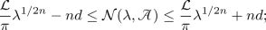  (3.7)

• (iii) the eigenvalues of satisfy the Weyl law

  

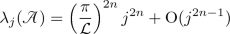  (3.8)

  as $j\rightarrow \infty$.

Proof

See “Appendix A.” $\square$

4 Transmission Matrices and the Secular Equation for n-Laplacians

In the spectral theory of Laplace operators on metric graphs, the main ingredient of the scattering matrix approach to parameterising the vertex conditions is that solutions to the equation $-\Delta \psi =k^2\psi$ on the edges can be written in a certain basis of incoming and outgoing waves: the corresponding amplitudes are related via the unitary vertex scattering matrix (see [35, 45]). For self-adjoint n-Laplacians, one may also introduce a $d\times d$ vertex scattering matrix (see Sect. 4.2), but for $n\ge 2$ it does not work as a parameter: vertex conditions are described by $n^2 d^2$ real parameters, whilst vertex scattering matrices contain just $d^2$ real parameters.

4.1 The Vertex Transmission Matrix

Let be an n-Laplacian in $L_2(\Gamma )$ satisfying Assumption 3.4. Throughout the rest of this paper, write $\omega :=\mathrm {e}^{\pi \mathrm {i}/n}$. Any function $\psi \in {{\widetilde{H}}}^{2n}(\Gamma )$ which satisfies the formal differential equation

$$\begin{aligned} (-\Delta )^n\psi =k^{2n}\psi \end{aligned}$$

(4.1)

on the edge $e(x_j)$ can be written in the form

$$\begin{aligned} \psi (x)=\sum _{l=0}^{n-1}a_j^l\mathrm {e}^{\mathrm {i}\omega ^lk|x-x_j|} +\sum _{l=0}^{n-1}b_j^l\mathrm {e}^{-\mathrm {i}\omega ^lk|x-x_j|},\qquad x\in e(x_j), \end{aligned}$$

(4.2)

for some amplitudes $a_j^l,b_j^l\in {\mathbb {C}}$ corresponding to the endpoint $x_j$. The terms with amplitudes $a_j^l$ serve as analogues of the incoming waves to the endpoint $x_j$ (from the scattering theory of Laplacians), and in the same way, the terms with amplitudes $b_j^l$ are the analogues of outgoing waves. Note that this analogy is purely formal since only the amplitudes with $l=0$ actually correspond to plane waves. Writing the amplitudes as column vectors ${\mathbf {a}}^l:=\{a_j^l\}_{j=1}^d$ and ${\mathbf {b}}^l:=\{b_j^l\}_{j=1}^d$ for $l=0,1,\dots ,n-1$, we can introduce a formal analogue of the vertex scattering matrix for general $n\in {\mathbb {N}}$, called the vertex transmission matrix. This is defined to be the $nd\times nd$ matrix ${\mathbb {T}}_\text {v}(k)$ such that a function $\psi$, which for each j has the form (4.2) in x in a neighbourhood of $x_j$, satisfies the vertex conditions of if and only if the amplitudes solve

$$\begin{aligned} \begin{pmatrix} {\mathbf {a}}^0\\ {\mathbf {a}}^1\\ \vdots \\ {\mathbf {a}}^{n-1} \end{pmatrix}={\mathbb {T}}_\text {v}(k)\begin{pmatrix}{\mathbf {b}}^0 \\ {\mathbf {b}}^1\\ \vdots \\ {\mathbf {b}}^{n-1}\end{pmatrix}. \end{aligned}$$

(4.3)

Note that this definition takes into account the vertex conditions only, and so we consider the amplitudes independently of whether they correspond to different endpoints of the same edge. This is necessary in order to be able to determine ${\mathbb {T}}_\text {v}(k)$ uniquely. We may write to avoid ambiguity.

The matrix can be constructed explicitly as follows: let $\psi \in L_2(\Gamma )$ be any function which in a neighbourhood of each vertex $x_j$ has the form (4.2). Then from the vertex conditions (3.6), we get the system of equations

$$\begin{aligned} {\mathbb {Y}}(k)\begin{pmatrix}{\mathbf {a}}^0\\ {\mathbf {a}}^1\\ \vdots \\ {\mathbf {a}}^{n-1}\end{pmatrix}=-{\mathbb {Y}}(-k)\begin{pmatrix}{\mathbf {b}}^0\\ {\mathbf {b}}^1\\ \vdots \\ {\mathbf {b}}^{n-1}\end{pmatrix}, \end{aligned}$$

(4.4)

where the $nd\times nd$ matrix ${\mathbb {Y}}(k)$ is defined for all $k\in {\mathbb {C}}$ by

$$\begin{aligned} {\mathbb {Y}}(k):=\left( \sum _{s=0}^{2n-1}(\mathrm {i}k)^s A_s\Bigg |\sum _{s=0}^{2n-1}(\mathrm {i}\omega k)^s A_s\Bigg |\cdots \Bigg |\sum _{s=0}^{2n-1}(\mathrm {i}\omega ^{n-1}k)^s A_s\right) . \end{aligned}$$

(4.5)

This matrix is clearly not unique for , but the associated linear relation (4.4) is uniquely determined. Wherever ${\mathbb {Y}}(k)$ is invertible, we then have

$$\begin{aligned} {\mathbb {T}}_\text {v}(k)=-{\mathbb {Y}}(k)^{-1}{\mathbb {Y}}(-k). \end{aligned}$$

(4.6)

In general, $\det {\mathbb {Y}}(k)$ may have nonzero roots which could be real, and thus, ${\mathbb {T}}_\text {v}(k)$ may be not everywhere defined on ${\mathbb {R}}$. Denote by the set of values of $k\in {\mathbb {C}}$ at which ${\mathbb {Y}}(k)$ is not invertible; it contains all singularities of ${\mathbb {T}}_\text {v}(k)$, but it should be noted that some of these singularities may be removable. We shall show that this set is finite.

Example 4.1

Consider the bi-Laplacian in $L_2([0,\infty ))$ with vertex conditions (3.6), where , , . It follows from Example 3.3 that it is self-adjoint. The matrix (4.5) is

$$\begin{aligned} {\mathbb {Y}}(k)=\begin{pmatrix}(1+\mathrm {i}k)(1-k^2) &{}\quad (1-k)(1+k^2) \\ \mathrm {i}k(1+k^2) &{}\quad -k(1-k^2)\end{pmatrix}. \end{aligned}$$

Now, $\det {\mathbb {Y}}(k)$ is a polynomial of degree five and has five distinct roots forming the set . It is clear for instance that , and one finds that this is a singularity of ${\mathbb {T}}_\text {v}$ which is not removable.

Lemma 4.2

Let be an n-Laplacian in $L_2(\Gamma )$. Under Assumption 3.4,

• (i) if $k\in {\mathbb {C}}\backslash \{0\}$, then if and only if there exists a non-trivial solution of (4.4) with ${\mathbf {b}}^l={\mathbf {0}}$ for all $l=0,\dots , n-1$;

• (ii) ,

• (iii) .

Proof

• (i): For $k\ne 0$, the matrix ${\mathbb {Y}}(k)$ is not invertible if and only if there exists a nonzero vector ${\mathbf {a}}$ such that ${\mathbb {Y}}(k){\mathbf {a}}={\mathbf {0}}$.

• (ii): It is clear from (4.5) that . Consider the d-star graph and on it the n-Laplacian with vertex conditions determined by . Suppose for a contradiction that is such that $\arg k\in (0,\frac{1}{2}\arg \omega )\cup (\frac{1}{2}\arg \omega ,\arg \omega )$. Now, part (i) implies that there exists a vector ${\mathbf {a}}$ satisfying (4.4) with ${\mathbf {b}}={\mathbf {0}}.$ By assumption, $\mathfrak {Re}[\mathrm {i}\omega ^lk]<0$ for all $l=0,\dots ,n-1$, so every $\psi$ decays exponentially along every half line (it is not identically zero on at least one of these). Thus, $\psi$ is an eigenfunction of the n-Laplacian operator on the d-star graph with the aforementioned vertex conditions. But by self-adjointness, the spectrum of this operator is real, and so, we get a contradiction since $k^{2n}\notin {\mathbb {R}}$.

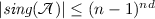
• (iii): By definition (4.5), it follows that $\det {\mathbb {Y}}(k)$ is a polynomial of degree at most $(n-1)^{nd}$. By part (ii), $\det {\mathbb {Y}}(k)\not \equiv 0$, and thus, it has at most $(n-1)^{nd}$ roots.

$\square$

Remark

Given a bi-Laplacian in $L_2(\Gamma )$, one can show that for , the operator is self-adjoint if and only if for some matrices ${\mathbf {S}},{\mathbf {B}},{\mathbf {C}},{\mathbf {D}}$ such that ${\mathbf {S}}{\mathbf {S}}^*={\mathbf {I}}$, ${\mathbf {S}}{\mathbf {C}}^*=\mathrm {i}{\mathbf {B}}$ and ${\mathbf {C}}{\mathbf {C}}^*=\mathrm {i}({\mathbf {D}}-{\mathbf {D}}^*)$. In principle, this can be generalised to parameterise higher-order n-Laplacians by ${\mathbb {T}}_\text {v}(k)$, but ${\mathbb {U}}(k)$ is a much more convenient parameter.

4.2 The Vertex Scattering Matrix

Given an n-Laplacian in $L_2(\Gamma )$ satisfying Assumption 3.4, denote by ${\mathbf {S}}_\text {v}(k)$ the upper left $d\times d$ block of ${\mathbb {T}}_\text {v}(k)$:

$$\begin{aligned} {\mathbb {T}}_\text {v}(k)=\begin{pmatrix}{\mathbf {S}}_\text {v}(k)&{}\quad *&{}\quad \ldots \\ *&{}\quad *&{}\quad \ldots \\ \vdots &{}\quad \vdots &{}\quad \ddots \end{pmatrix}. \end{aligned}$$

(4.7)

This is the matrix which relates the amplitudes ${\mathbf {a}}^0$ and ${\mathbf {b}}^0$ of classical incoming and outgoing plane waves $\mathrm {e}^{\mathrm {i}k|x-x_j|}$ and $\mathrm {e}^{-\mathrm {i}k|x-x_j|}$, respectively. We refer to ${\mathbf {S}}_\text {v}(k)$ as the vertex scattering matrix of . If there is ambiguity, we may write it as . One can show that it is unitary on ${\mathbb {R}}$ and is thus defined even when ${\mathbb {T}}_\text {v}(k)$ is not: since each entry of ${\mathbf {S}}_\text {v}(k)$ is then a bounded rational function of k on , it can be extended to all of ${\mathbb {R}}$ by taking limits. The proof of this is elementary but messy, so we defer it to “Appendix B.”

Theorem 4.3

Let be an n-Laplacian in $L_2(\Gamma )$. Under Assumption 3.4, the vertex scattering matrix ${\mathbf {S}}_v (k)$ is unitary for all $k\in {\mathbb {R}}$.

Proof

See “Appendix B.” $\square$

This fact is not surprising since the vertex scattering matrix as we define it coincides with the scattering matrix from the mathematical scattering theory (see [57]) for a certain pair of operators on the non-compact star graph with different vertex conditions. This matrix will play a key role in analysing the spectral asymptotics (see Sect. 6). In the case of the bi-Laplacian ($n=2$) for instance, given a physical network of beams, it should be possible to measure ${\mathbf {S}}_\text {v}(k)$ for certain values of k by generating plane waves far along each beam and measuring how these are scattered: for solutions with ${\mathbf {b}}^1 = {\mathbf {0}}$, we have ${\mathbf {a}}^0={\mathbf {S}}_\text {v}(k){\mathbf {b}}^0$. However, unlike in the Laplacian case, in general for $n\ge 2$, knowledge of ${\mathbf {S}}_\text {v}(k)$ alone is not sufficient to determine the vertex conditions. Nevertheless, if one can be sure that the vertex conditions are scaling-invariant (Sect. 5), then one can determine a lot more about the vertex conditions from ${\mathbf {S}}_\text {v}(k)$ (e.g. Corollary 5.4) even though we shall see that for such conditions the matrix is constant.

4.3 The Edge Transmission Matrix

Let be an n-Laplacian in $L_2(\Gamma )$ satisfying Assumption 3.4, and suppose, as we shall for the remainder of the paper, that all $N=d/2$ edges are compact. A function $\psi$ is an eigenfunction of if and only if it satisfies the differential equation (4.1) on the edges, together with the vertex conditions. Every such function can be written as (4.2) for all $x\in e(x_j)$. The amplitudes $a_j^l, b_j^l$ are not independent: one connection comes from the vertex conditions (c.f. (4.3)); the other comes from the edges. On each (compact) edge, $\psi$ has two expressions, one associated with each endpoint. These expressions match if and only if

$$\begin{aligned} \begin{aligned} a_j^l&=b_{j+N}^l\mathrm {e}^{-\mathrm {i}\omega ^lk\ell _j},\\ b_j^l&= a_{j+N}^l\mathrm {e}^{+\mathrm {i}\omega ^lk\ell _j}, \end{aligned} \end{aligned}$$

(4.8)

for all $j=1,\dots ,N=d/2$, where $\ell _j$ is the length of edge $e_j$ (c.f., for example, [28]). This can be encoded into an $nd\times nd$ matrix ${\mathbb {T}}_\text {e}(k)$ (like the edge scattering matrix for Laplacians, c.f. [45]) such that the expressions match if and only if

$$\begin{aligned} {\mathbb {T}}_\text {e}(k)\begin{pmatrix}{\mathbf {a}}^0\\ {\mathbf {a}}^1\\ \vdots \\ {\mathbf {a}}^{n-1}\end{pmatrix} =\begin{pmatrix}{\mathbf {b}}^0\\ {\mathbf {b}}^1\\ \vdots \\ {\mathbf {b}}^{n-1}\end{pmatrix}. \end{aligned}$$

(4.9)

We refer to ${\mathbb {T}}_\text {e}(k)$ as the edge transmission matrix corresponding to the set of edges E. It is independent of the vertex conditions of and hence also independent of the topology of the induced graph . It is clear from (4.8) that this matrix is given explicitly by

$$\begin{aligned} {\mathbb {T}}_\text {e}(k)=\begin{pmatrix}{\mathbf {S}}_\text {e}(k)&{}\quad 0&{}\quad \ldots &{}\quad 0\\ 0&{}\quad {\mathbf {S}}_\text {e}(\omega k)&{}\quad \ldots &{}\quad 0\\ \vdots &{}\quad \vdots &{}\quad \ddots &{}\quad \vdots \\ 0&{}\quad 0&{}\quad \ldots &{}\quad {\mathbf {S}}_\text {e}(\omega ^{n-1}k)\end{pmatrix}, \end{aligned}$$

(4.10)

where

$$\begin{aligned} {\mathbf {S}}_\text {e}(k):=\begin{pmatrix}0&{}\quad \mathrm {e}^{\mathrm {i}k\Lambda }\\ \mathrm {e}^{\mathrm {i}k\Lambda }&{}\quad 0\end{pmatrix}, \end{aligned}$$

(4.11)

and $\Lambda :=\text {diag}(\ell _1,\dots ,\ell _N)$ is the diagonal matrix whose nonzero entries are the lengths of the (compact) edges. Comparing with [45], we see that ${\mathbf {S}}_\text {e}(k)$ is precisely the edge scattering matrix for Laplacians on the same set E of edges.

4.4 The Secular Equation

Theorem 4.4

Let be an n-Laplacian in $L_2(\Gamma )$, and suppose that all of the edges in E are compact. Under Assumption 3.4, nonzero spectrum of is given by the set of solutions $\lambda =k^{2n}$ to the equation

$$\begin{aligned} \det [{\mathbb {Y}}(k)+{\mathbb {Y}}(-k){\mathbb {T}}_e (k)]=0, \end{aligned}$$

(4.12)

where ${\mathbb {Y}}(k)$ is expressed as (4.5) in terms of the vertex conditions (3.6), and the geometric multiplicity of $\lambda$ equals the dimension of $\ker [{\mathbb {Y}}(k)+{\mathbb {Y}}(-k){\mathbb {T}}_\text {e}(k)]$. Those values of k that are not in are equivalently the solutions of

$$\begin{aligned} \det [{\mathbb {I}}-{\mathbb {T}}_v (k){\mathbb {T}}_e (k)]=0. \end{aligned}$$

(4.13)

Proof

We saw in Sect. 4.1 that a nonzero function $\psi$ of the form (4.2) in a neighbourhood of each endpoint $x_j$ satisfies the vertex conditions of if and only if the amplitudes satisfy (4.4). Moreover, as all edges are compact, we saw in Sect. 4.2 that (4.9) must hold. Thus, $\psi$ is an eigenvector of if and only if both of these hold, equivalently, if and only if

$$\begin{aligned} {[}{\mathbb {Y}}(k)+{\mathbb {Y}}(-k){\mathbb {T}}_\text {e}(k)] \begin{pmatrix}{\mathbf {a}}^0\\ \vdots \\ {\mathbf {a}}^{n-1}\end{pmatrix}=0. \end{aligned}$$

(4.14)

A non-trivial vector solution of this equations exists if and only if k solves (4.12). In other words, $\lambda \ne 0$ is an eigenvalue of if and only $\lambda =k^{2n}$ for some solution k of (4.12) which one may assume without loss of generality is such that $\arg k\in [0,\pi /n)$.

It remains only to check multiplicities. On each edge $e_j$, where $j=1,\dots ,N$ ($=d/2$), there is a bijection between the amplitudes $a_j^0\dots ,a_j^{n-1},b_j^0,\dots ,b_j^{n-1}$ and solutions of the eigenvalue problem $(-\Delta )^n\psi _j=\lambda \psi _j$ on that edge. Moreover, it follows from the relations (4.8) that there is a bijective correspondence between the amplitudes $a_j^0,a_{j+N}^0,\dots ,a_j^{n-1},a_{j+N}^{n-1}$ associated with that edge and the solutions of the eigenvalue problem along that edge via (4.2). Hence, the vector solutions of equation (4.14) for fixed $\arg k$ are in bijection with the $\lambda =k^{2n}$ eigenstates of the n-Laplacian. $\square$

Example 4.5

Consider the bi-Laplacian in $L_2([0,\ell ])$ with the same vertex conditions as the operator from Example 4.1, but now applied at both endpoints. One has

$$\begin{aligned} {\mathbb {Y}}(k)&=\begin{pmatrix}(1+\mathrm {i}k)(1-k^2){\mathbf {I}} &{}\quad (1-k)(1+k^2){\mathbf {I}} \\ \mathrm {i}k(1+k^2){\mathbf {I}} &{}\quad -k(1-k^2){\mathbf {I}}\end{pmatrix},\\ {\mathbb {T}}_\text {e}(k)&=\begin{pmatrix}0&{}\quad \mathrm {e}^{\mathrm {i}k\ell }&{}\quad 0&{}\quad 0\\ \mathrm {e}^{\mathrm {i}k\ell }&{}\quad 0&{}\quad 0&{}\quad 0\\ 0&{}\quad 0&{}\quad 0&{}\quad \mathrm {e}^{-k\ell }\\ 0&{}\quad 0&{}\quad \mathrm {e}^{-k\ell }&{}\quad 0\end{pmatrix}. \end{aligned}$$

The nonzero eigenvalues are then the values $k^2$ for which k solves (4.12). It follows from Example 4.1 that $k=1$ is an irremovable singularity of ${\mathbb {T}}_\text {v}(k)$ for this operator as well. However, one finds that if $\ell =\pi$, then $k=1$ will be a root of (4.12). Hence, in this case, one could not pick up the eigenvalue 1 using the alternative equation (4.13).

Equation (4.13) serves as a secular equation for , although the finite number of possible instances where solutions of (4.12) coincide with singularities of ${\mathbb {T}}_\text {v}(k)$ must be taken into account. It is a generalisation of the secular equation for self-adjoint Laplacians which has the form $\det [{\mathbf {I}}-{\mathbf {S}}_\text {v}(k){\mathbf {S}}_\text {e}(k)]=0$, where ${\mathbf {S}}_\text {v}(k)$ and ${\mathbf {S}}_\text {e}(k)$ are the vertex scattering matrix and the edge scattering matrix respectivey for (see, for example, [28, 35, 44]). Much more can be said about the spectrum of in the case that ${\mathbf {S}}_\text {v}$ is independent of k—corresponding to so-called scaling-invariant vertex conditions—which is largely due to the fact that in this case, the determinant is a trigonometric polynomial (see, for example, [47]). It would then be a natural step to study the n-Laplacians whose vertex conditions are such that ${\mathbb {T}}_\text {v}$ is independent of k. In that case, so equation (4.13) would give all of the (nonzero) eigenvalues of .

Remark

Whilst one could similarly derive a secular equation in terms of the unitary parameter ${\mathbb {U}}$, thereby avoiding the issue of singularities, the corresponding (non-unitary) matrix for the edges is less versatile than ${\mathbb {T}}_\text {e}$ due to the particular choice of basis of solutions of (4.1) needed (c.f. “Appendix B”).

5 Scaling-Invariant Vertex Conditions

Definition

The vertex conditions of differential operator in $L_2(\Gamma )$ are called scaling-invariant if and only if, for any $c>0$, $\psi (x)$ satisfies the vertex conditions on $\Gamma$ whenever $\psi (cx)$ does on $c\Gamma$.

Scaling-invariant vertex conditions have the characterising property that $\lambda$ is an eigenvalue of an n-Laplacian on E with such conditions if and only if $c^{2n}\lambda$ is an eigenvalue of the n-Laplacian on cE with the same vertex conditions.

Given an n-Laplacian in $L_2(\Gamma )$, not necessarily self-adjoint, its vertex conditions (2.5) are scaling-invariant (i.e. hold independently of the choice of scaling $c>0$) if and only if they can equivalently be written

$$\begin{aligned}&\sum _{r=0}^{2n-1} c^r A_r \partial ^r \Psi = 0,\quad \forall c>0 \nonumber \\&\quad \Rightarrow A_0\varvec{\Psi }= A_1\partial \varvec{\Psi }=\dots = A_{2n-1}\partial ^{2n-1}\varvec{\Psi }=0. \end{aligned}$$

(5.1)

Thus, is a product of first-order differential operators, and in the notation of Sect. 2.2, it can be expressed as

On the other hand, any operator of this form is an n-Laplacian with scaling-invariant vertex conditions. We seek the subset of these which are also self-adjoint.

Remark

For Laplacians ($n=1$), the vertex conditions are scaling-invariant if and only if the so-called Robin part of the associated quadratic form vanishes (Theorem 2.1.6, [8]): these are precisely the Laplacians which can be written as a product of a first-order operator and its adjoint. More generally, we claim (though shall not prove in this paper) that self-adjoint n-Laplacians with non-Robin vertex conditions are those which can be written in the form for some nth derivative operator . Then the following theorem will imply that for $n\ge 2$ scaling-invariant vertex conditions do not give all non-Robin n-Laplacians.

Theorem 5.1

Let be an n-Laplacian in $L_2(\Gamma )$ with vertex conditions (3.6) and let $k\in {\mathbb {R}}\backslash \{0\}$. Under Assumption 3.4, the following are equivalent:

• (a) has scaling-invariant vertex conditions,

• (b) for some first-order differential operators in $L_2(\Gamma )$,³

• (c) $A_0 A_{2n-1}^*= A_1 A_{2n-2}^*=\dots = A_{n-1} A_n^*=0$,

• (d) ${\mathbb {U}}$ is independent of k,

• (e) ${\mathbb {T}}_v$ is independent of k,

• (f) there exist $d\times d$ unitary Hermitian matrices ${\mathbf {U}}_1,\dots ,{\mathbf {U}}_n$ such that

  $$\begin{aligned} {\mathbb {U}}(k)=\begin{pmatrix}{\mathbf {U}}_1&{}\quad 0&{}\quad \ldots &{}\quad 0\\ 0&{}\quad -{\mathbf {U}}_2&{}\quad \ldots &{}\quad 0\\ \vdots &{}\quad \vdots &{}\quad \ddots &{}\quad \vdots \\ 0&{}\quad 0&{}\quad \ldots &{}\quad (-1)^{n-1}{\mathbf {U}}_n\end{pmatrix}. \end{aligned}$$

  (5.2)

In this case, ${\mathbf {U}}_j$ is the vertex scattering matrix of the Laplacian

Proof

(a)$\Leftrightarrow$(b)$\Leftrightarrow$(c): Recall that has scaling-invariant vertex conditions if and only if the operator can be decomposed in the following way:

in the notation of Sect. 2.2. Then is self-adjoint and scaling-invariant if and only if additionally for all j, which by Lemma 2.1 is if and only if $A_j A_{2n-1-j}^*=0$ (and $\text {rank}( A_j)+\text {rank}( A_{2n-1-j})=d$).

(c)$\Rightarrow$(d),(f): The vertex conditions can be written ${\mathbb {A}}(k)\varvec{\Gamma }_0(k)\psi ={\mathbb {B}}(k)\varvec{\Gamma }_1(k)\psi$ for each $k\in {\mathbb {R}}\backslash \{0\}$, where ${\mathbb {A}}(k),{\mathbb {B}}(k)$ are defined by (A.2) in the proof of Theorem 3.2. If (c) holds, then one can assume without loss of generality that the ${\mathbb {A}}(k),{\mathbb {B}}(k)$ are block diagonal with blocks of size $d\times d$, and in particular, ${\mathbb {A}}(k){\mathbb {B}}(k)^*=0$. But since these vertex conditions are also equivalent to (3.3), there exists ${\mathbb {X}}\in \text {GL}(nd)$ such that ${\mathbb {X}}{\mathbb {A}}(k)=\mathrm {i}({\mathbb {U}}(k)-{\mathbb {I}})$ and ${\mathbb {X}}{\mathbb {B}}(k)={\mathbb {U}}(k)+{\mathbb {I}}$. Then ${\mathbb {A}}(k){\mathbb {B}}(k)^*=0$ implies that ${\mathbb {U}}(k)={\mathbb {U}}(k)^*$. It then follows from (A.5) that ${\mathbb {U}}(k)$ has the form (5.2). Moreover, (c) implies that in fact (A.3) and (A.4) hold for all (complex) $k\in {\mathbb {C}}\backslash \{0\}$, whence ${\mathbb {U}}(k)$ is unitary for all $k\in {\mathbb {C}}$, and by (A.5), it is holomorphic. Liouville’s theorem then implies that it must be constant.

(d)$\Leftrightarrow$(e): See Corollary B.2.

(d)$\Rightarrow$(a): By Theorem 3.2, the vertex conditions can be written in the form $\mathrm {i}({\mathbb {U}}(k)-{\mathbb {I}})\varvec{\Gamma }_0(k) \psi =({\mathbb {U}}(k)+{\mathbb {I}})\varvec{\Gamma }_1(k)\psi$ for every $k\in {\mathbb {R}}\backslash \{0\}$. If ${\mathbb {U}}$ is independent of k, then this implies that ${\mathbb {U}}$ must be block diagonal, consisting of blocks of size $d\times d$, and that in fact $\mathrm {i}({\mathbb {U}}-{\mathbb {I}})\varvec{\Gamma }_0(k)\psi =({\mathbb {U}} +{\mathbb {I}})\varvec{\Gamma }_1(k)\psi =0$ for all $k\in {\mathbb {R}}\backslash \{0\}$. Hence, the vertex conditions are scaling-invariant (c.f. (5.1)).

(f)$\Rightarrow$(a): If ${\mathbb {U}}(k)$ is of the form (5.2), then it is clear from the fact that the vertex conditions can be written in the form (3.3) that they are scaling-invariant (c.f. (5.1)).

Finally, suppose that any and thus all of the above hold. Then we have for some first-order operators . Now, the vertex conditions for can be written explicitly as

$$\begin{aligned} \begin{aligned} ({\mathbf {U}}_1-{\mathbf {I}})\varvec{\Psi }&=({\mathbf {U}}_1+{\mathbf {I}})\partial ^{2n-1}\varvec{\Psi }=0,\\ ({\mathbf {U}}_2-{\mathbf {I}})\partial ^{2n-2}\varvec{\Psi }&=({\mathbf {U}}_2+{\mathbf {I}})\partial \varvec{\Psi }=0,\\ ({\mathbf {U}}_3-{\mathbf {I}})\partial ^2\varvec{\Psi }&=({\mathbf {U}}_3+{\mathbf {I}})\partial ^{2n-3}\varvec{\Psi }=0,\\&\vdots \\ \end{aligned} \end{aligned}$$

and the non-Robin Laplacians have vertex conditions

$$\begin{aligned} ({\mathbf {U}}_1-{\mathbf {I}})\varvec{\Psi }&=({\mathbf {U}}_1+{\mathbf {I}})\partial \varvec{\Psi }=0,\\ ({\mathbf {U}}_2-{\mathbf {I}})\varvec{\Psi }&=({\mathbf {U}}_2+{\mathbf {I}})\partial \varvec{\Psi }=0,\\ ({\mathbf {U}}_3-{\mathbf {I}})\varvec{\Psi }&=({\mathbf {U}}_3+{\mathbf {I}})\partial \varvec{\Psi }=0,\\&\vdots \end{aligned}$$

respectively. Thus, ${\mathbf {U}}_1,{\mathbf {U}}_2,{\mathbf {U}}_3,\dots$ must be their respective vertex scattering matrices (c.f. Theorem 3.2, or specifically for Laplacians: Theorem 2.1 in [45]). $\square$

Example 5.2

Let $\Gamma$ be a compact finite metric graph with vertices V, and let be the bi-Laplacian in $L_2(\Gamma )$ with vertex conditions:

$$\begin{aligned} \left\{ \begin{array}{l}\psi (x_j)=\psi (x_{j'})\ \forall x_j,x_{j'}\in v_m,\\ \partial \psi (x_j)=0\ \forall x_j\in v_m,\\ \partial ^2\psi (x_j)\text { arbitrary }\forall x_j\in v_m,\\ \sum _{x_j\in v_m}\partial ^3\psi (x_j)=0,\end{array}\right. \end{aligned}$$

for all vertices $v_m\in V$. Note that no conditions are imposed on the second derivates. This operator is the Friedrichs extension of the symmetric operator whose only conditions are continuity of functions at the vertices of $\Gamma$ (see Example 4.5 in [27]). Clearly these vertex conditions are scaling-invariant: in particular using the notation from Sect. 2.2. The unitary parameter for is

where ${\mathbf {S}}_\text {st}$ is the vertex scattering matrix for the standard Laplacian mentioned in Sect. 2.2.

The remainder of the paper is focused on the situation in which the vertex transmission matrix ${\mathbb {T}}_\text {v}$ is independent of k. To ensure that this is the case, according to Theorem 5.1, we shall work with n-Laplacians satisfying Assumption 3.4 together with the following:

Assumption 5.3

The vertex conditions are scaling-invariant, and all edges are compact.

For bi-Laplacians satisfying these assumptions, one can establish the following relationship between the unitary parameter ${\mathbb {U}}$ and the vertex scattering matrix ${\mathbf {S}}_\text {v}$. It can be generalised for higher-order operators, but the computations become more involved so we do not present that here.

Corollary 5.4

Let be a bi-Laplacian in $L_2(\Gamma )$ satisfying Assumptions 3.4 and 5.3. Let ${\mathbf {S}}_v$ be the vertex scattering matrix for , and let ${\mathbf {U}}_1$ and $-{\mathbf {U}}_2$ be the unitary Hermitian diagonal blocks of the unitary parameter ${\mathbb {U}}$ as given by (5.2). Then $\mathrm {i}{\mathbf {I}}+{\mathbf {S}}_v$ is invertible, and

$$\begin{aligned} {\mathbf {U}}_1+{\mathbf {U}}_2=-2\mathrm {i}(\mathrm {i}{\mathbf {I}} -{\mathbf {S}}_v )(\mathrm {i}{\mathbf {I}}+{\mathbf {S}}_v )^{-1}. \end{aligned}$$

(5.3)

In particular, ${\mathbf {S}}_v$ is the vertex scattering matrix for a self-adjoint scaling-invariant bi-Laplacian if and only if there exist unitary Hermitian matrices ${\mathbf {U}}_1$ and ${\mathbf {U}}_2$ such that ${\mathbf {S}}_v =\mathrm {i}\{2{\mathbf {I}}+\mathrm {i}({\mathbf {U}}_1 +{\mathbf {U}}_2)\}^{-1}\{2{\mathbf {I}}-\mathrm {i}({\mathbf {U}}_1+{\mathbf {U}}_2)\}$. It is determined uniquely by the sum ${\mathbf {U}}_1+{\mathbf {U}}_2$ and thus corresponds to every bi-Laplacian with unitary Hermitian parameter such that (5.3) holds. Moreover:

• (i) ${\mathbf {S}}_v ={\mathbf {S}}_v ^*$ if and only if ${\mathbf {U}}_1={\mathbf {U}}_2$, and in this case ${\mathbf {S}}_v ={\mathbf {U}}_1={\mathbf {U}}_2$,

• (ii) ${\mathbf {S}}_v =\mathrm {i}{\mathbf {I}}$ if and only if ${\mathbf {U}}_1=-{\mathbf {U}}_2$.

Proof

See “Appendix B.” $\square$

Remark

If ${\mathbf {U}}_1$ and ${\mathbf {U}}_2$ are unitary Hermitian matrices, then $({\mathbf {U}}_1-{\mathbf {U}}_2)^2=4{\mathbf {I}} -({\mathbf {U}}_1+{\mathbf {U}}_2)^2$. Hence, one can use equation (5.3) to compute $({\mathbf {U}}_1-{\mathbf {U}}_2)^2$ in terms of ${\mathbf {S}}_\text {v}$. However, in general this is not sufficient to obtain ${\mathbf {U}}_1$ and ${\mathbf {U}}_2$, and so, ${\mathbf {S}}_\text {v}$ does not uniquely determine the corresponding bi-Laplacian.

6 The Secular Equation for Scaling-Invariant Vertex Conditions

6.1 More on the Secular Equation

For an n-Laplacian in $L_2(\Gamma )$ satisfying Assumptions 3.4 and 5.3, the vertex transmission matrix ${\mathbb {T}}_\text {v}$ is independent of k (Theorem 5.1), in which case the ‘secular equations’ (4.12) and (4.13) from Theorem 4.4 are completely equivalent. We thus refer to the function

(6.1)

as the secular function for , and the equation $\chi =0$ as the secular equation.

Let us decompose the transmission matrices ${\mathbb {T}}_\text {v}$ and ${\mathbb {T}}_\text {e}(k)$ into blocks in the following way:

$$\begin{aligned} {\mathbb {T}}_\text {v}=\begin{pmatrix}{\mathbf {S}}_\text {v}&{}\quad B_\text {v}\\ C_\text {v}&{} \quad {\tilde{T}}_\text {v}\end{pmatrix},\qquad {\mathbb {T}}_\text {e}(k) =\begin{pmatrix}{\mathbf {S}}_\text {e}(k)&{}\quad 0\\ 0&{}\quad {\tilde{T}}_\text {e}(k)\end{pmatrix}. \end{aligned}$$

(6.2)

The $(n-1)d\times (n-1)d$ matrix ${\tilde{T}}_\text {e}(k)$ consists of sub-blocks of the form ${\mathbf {S}}_\text {e}(\omega ^lk)$ for $l\ge 1$, where we recall that $\omega :=\mathrm {e}^{\pi \mathrm {i}/n}$. This means that if $n\ge 2$, then the secular function is in general not a trigonometric polynomial like it is for Laplacians. The upside is that only ${\mathbf {S}}_\text {e}(k)$ has much influence on the secular equation for large k since ${\tilde{T}}_\text {e}(k)\rightarrow 0$ exponentially as $k\rightarrow \infty$. Indeed, dividing $\chi (k)$ by an appropriate function (see Lemma 6.1) we get

(6.3)

where . One needs to be careful in specifying where F is well defined, but then equation $F=0$ is almost equivalent to the secular equation:

Lemma 6.1

Let be an n-Laplacian in $L_2(\Gamma )$. Under Assumptions 3.4 and 5.3, for any $\theta \in (0,\frac{\pi }{n})$, there exists $\gamma _\theta \ge 0$ such that the function F is well defined in the sector $\{z\in {\mathbb {C}}:|\arg (z-\gamma _\theta )|<\theta \}$, and has the same roots as the secular function $\chi$ counting multiplicities.

Proof

For $l=1,\dots ,n-1$, we have $|\mathrm {e}^{\mathrm {i}\omega ^lk}|=\mathrm {e}^{-|k|\sin (\frac{\pi l}{n}+\arg k)}\le \mathrm {e}^{-|k|\sin (\frac{\pi }{n}-\theta )}$ on the sector $|\arg k|<\theta$. Then ${\tilde{T}}_\text {e}(k)$ consists of exponentially decreasing blocks ${\mathbf {S}}_\text {e}(\omega ^lk)$ for $l=1,\dots ,n-1$, so as ${\tilde{T}}_\text {v}$ is independent of k, there certainly exists $\gamma _\theta >0$ such that the function

$$\begin{aligned} {\tilde{F}}(k):=\det [I_{(n-1)d}-{\tilde{T}}_\text {v}{\tilde{T}}_\text {e}(k)] \end{aligned}$$

(6.4)

is bounded below by $\frac{1}{2}$ on the shifted sector $|\arg (z-\gamma _\theta )|\le \theta$ and thus has no zeros there. Then ${\mathbf {X}}(k)$ is well defined in this sector, and hence so is F. Since $\chi (k)=F(k){\tilde{F}}(k)$, the result follows. $\square$

6.2 The Associated Trigonometric Polynomial and Dirac Operator

Due to the exponentially decreasing nature of the matrix ${\mathbf {X}}(k)$, the function F(k) is in some sense very close to the trigonometric polynomial

(6.5)

This looks very much like the secular function for a self-adjoint Laplacian, but in general this is not the case: despite being a constant unitary matrix, ${\mathbf {S}}_\text {v}$ is not necessarily Hermitian (c.f. Theorem 2.1.6, [8]). For instance, by Corollary 5.4, the scattering matrix for a self-adjoint bi-Laplacian with scaling-invariant conditions is Hermitian if and only if is the square of a Laplacian. Nevertheless, the equation $G=0$ is still the secular equation of a self-adjoint differential operator: given a $d\times d$ unitary matrix ${\mathbf {U}}$, consider the Dirac operator

(6.6)

Its spectrum is given by the roots of the secular function $\det [{\mathbf {I}}-{\mathbf {U}}{\mathbf {S}}_\text {e}(k)]$. In the case that ${\mathbf {U}}:={\mathbf {S}}_\text {v}$ (6.5) is its secular function.

As G is a trigonometric polynomial with fewer terms, its roots are easier to compute than those of F, and one would hope to be able to use them to asymptotically approximate the eigenvalues of . More precisely, one would expect that the roots of F become asymptotically closer to the roots of G. To prove such a result for two functions f and g, we would need to compute integrals of $f'/f-g'/g$ along progressively smaller contours around more and more distant roots, and show that these are zero. One would therefore hope that they satisfy

$$\begin{aligned} \lim _{\begin{array}{c} |z|\rightarrow \infty \\ z\in {\mathcal {U}} \end{array}}|f(z)-g(z)|=0, \qquad \lim _{\begin{array}{c} |z|\rightarrow \infty \\ z\in {\mathcal {U}} \end{array}}|f'(z)-g'(z)|=0 \end{aligned}$$

(6.7)

for some appropriate (unbounded) open set ${\mathcal {U}}$. The sort of ‘appropriate set’ that we shall work with is what we refer to as a right half strip, namely anything of the form

$$\begin{aligned} {\mathcal {U}}=\{z\in {\mathbb {C}}:\mathfrak {Re}\,z>\gamma ,\,a<\mathfrak {Im}\,z<b\}, \end{aligned}$$

(6.8)

for $a,b,\gamma \in {\mathbb {R}}$.

Definition

If g is a trigonometric polynomial, or more generally an almost periodic function, then we shall refer to any holomorphic function f satisfying (6.7) as a holomorphic perturbation of g on ${\mathcal {U}}$.

For a complete proof of convergence of the roots of such functions, we need some results from the theory of almost periodic functions (see Sect. 7). The next lemma ensures that this theory would indeed be applicable to F and G.

Lemma 6.2

Let be an n-Laplacian in $L_2(\Gamma )$. Under Assumptions 3.4 and 5.3, the function is a holomorphic perturbation of on any right half strip ${\mathcal {U}}$.

Proof

Fix $\theta \in (0,\frac{\pi }{n})$. It is sufficient to prove this result for any half strip which is contained in the sector $\{z\in {\mathbb {C}}:|\arg (z-\gamma _\theta )|\le \theta \}$; recall from Lemma 6.1 that $\gamma _\theta \ge 0$ was chosen such that the function ${\tilde{F}}$ defined by (6.4) satisfies $|{\tilde{F}}|\ge \frac{1}{2}$ here.

Let ${\mathcal {Q}}$ be the following set of holomorphic functions defined on this sector:

$$\begin{aligned} {\mathcal {Q}}:=\left\{ k\mapsto \frac{1}{{\tilde{F}}(k)^a}\sum _{m=1}^Mc_m\mathrm {e}^{\mathrm {i}\zeta _mk}\;\Bigg |\;\begin{array}{l} a,M\in {\mathbb {N}},\\ c_m\in {\mathbb {C}},\\ \zeta _m\in {\mathbb {H}}_+ \end{array} \right\} , \end{aligned}$$

where ${\mathbb {H}}_+$ denotes the upper half plane. Observe that ${\mathcal {Q}}$ is invariant under differentiation and multiplication by trigonometric polynomials. Given some $h(k)={\tilde{F}}(k)^{-a}\sum _{m=1}^Mc_m\mathrm {e}^{\mathrm {i}\zeta _mk}\in {\mathcal {Q}}$, as $\mathfrak {Im}\,k$ is bounded on ${\mathcal {U}}$ there exists a constant $C_{h}>0$ such that $|\mathrm {e}^{\mathrm {i}(\mathfrak {Re}\,\zeta _m)k}|=\mathrm {e}^{-(\mathfrak {Re}\,\zeta _m)\mathfrak {Im}\,k}\le C_{h}$ for $m=1,\dots ,M$ whenever $k\in {\mathcal {U}}$. Then $|h(k)|\le 2^aC_{h}\sum _{m=1}^M |c_m| \mathrm {e}^{-(\mathfrak {Im}\,\zeta _m)\mathfrak {Re}\,k}$, so $h\rightarrow 0$ as $|k|\rightarrow 0$ on ${\mathcal {U}}$. To complete the proof, it is thus sufficient to show that $F-G\in {\mathcal {Q}}$.

Recall from definitions (6.3) and (6.5) that $F(k)=\det [({\mathbf {I}}-{\mathbf {S}}_\text {v}{\mathbf {S}}_\text {e}(k))-{\mathbf {X}}(k)]$ and $G(k)=\det [{\mathbf {I}}-{\mathbf {S}}_\text {v}{\mathbf {S}}_\text {e}(k)]$. The entries of the matrix ${\mathbf {X}}(k)$ are all from ${\mathcal {Q}}$, whilst all entries of ${\mathbf {I}}-{\mathbf {S}}_\text {v}{\mathbf {S}}_\text {e}(k)$ are trigonometric polynomials. Now, the expression

$$\begin{aligned} \det [({\mathbf {I}}-{\mathbf {S}}_\text {v}{\mathbf {S}}_\text {e}(k))-{\mathbf {X}}(k)] \end{aligned}$$

can be written as a sum of determinants of matrices formed from combinations of rows of ${\mathbf {I}}-{\mathbf {S}}_\text {v}{\mathbf {S}}_\text {e}(k)$ and ${\mathbf {X}}(k)$. The only one of these determinants which does not involve rows of ${\mathbf {X}}(k)$ is equal to G(k) itself; the other determinants are thus all elements of ${\mathcal {Q}}$. Then $F-G\in {\mathcal {Q}}$ as required. $\square$

6.3 Multiplicity of Eigenvalues

Given an eigenvalue $\lambda =k^{2n}$ of , we refer to the dimension of the $\lambda$ eigenspace as the geometric multiplicity of $\lambda$ and the order of k as a root of the secular function as the algebraic multiplicity of $\lambda$.⁴ As usual, assume that satisfies Assumption 5.3. Now, Lemma 6.1 implies that the algebraic multiplicity is equal to the order of k as a root of F, provided that $k>\gamma _\theta$. Ideally, one would prove that the latter equals the geometric multiplicity of the eigenvalue. Of course, one can easily show that geometric multiplicity is at most equal to algebraic multiplicity:

Lemma 6.3

Let be an n-Laplacian in $L_2(\Gamma )$. Under Assumptions 3.4 and 5.3, the geometric multiplicity of any positive eigenvalue $\lambda >0$ of is at most equal to its algebraic multiplicity.

Proof

Let $\lambda =k_0^{2n}$ be an eigenvalue of with geometric multiplicity M. The matrix ${\mathbb {I}}-{\mathbb {T}}_\text {v}{\mathbb {T}}_\text {e}(k_0)$ has rank $n-M$; in other words, any set of $n-M+1$ of its columns is linearly dependent. Now, for each $j=1,\dots ,M-1$, the jth derivative of (6.1),

$$\begin{aligned} \frac{\mathrm {d}^j}{\mathrm {d}k^j}\chi (k)\equiv \frac{\mathrm {d}^j}{\mathrm {d}k^j}\det [{\mathbb {I}}-{\mathbb {T}}_\text {v}{\mathbb {T}}_\text {e}(k)], \end{aligned}$$

can be written as a sum of determinants of matrices each of which contains at least $n-j$ columns of the matrix ${\mathbb {I}}-{\mathbb {T}}_\text {v}{\mathbb {T}}_\text {e}(k)$. Thus, at $k=k_0$, the jth derivative of F vanishes. Hence, $k_0$ is a zero of $\chi$ of order at least M. $\square$

It would be convenient to be able to see equality of these multiplicities in the same way as one can for Laplacians (see, for example, Theorem 3.7.1, [8]) or, more usefully for us, the Dirac operator :

Lemma 6.4

The geometric multiplicity of any positive eigenvalue $k>0$ of the Dirac operator , defined by (6.6), is equal to its algebraic multiplicity as a root of the secular function $\det [{\mathbf {I}}-{\mathbf {U}}{\mathbf {S}}_e (k)]$.

Proof

The proof is identical to the proof of Theorem 3.7.1 in [8]: the eigenvalues $\mathrm {e}^{\mathrm {i}\theta _j(k)}$ of the matrix ${\mathbf {U}}{\mathbf {S}}_\text {e}(k)$ satisfy $\det [{\mathbf {I}}-{\mathbf {U}}{\mathbf {S}}_\text {e}(k)]= \prod _{j=1}^d(1-\mathrm {e}^{\mathrm {i}\theta _j(k)})$. By unitarity of ${\mathbf {U}}$, one has $\frac{\mathrm {d}\theta _j}{\mathrm {d}k}>0$ for every j according to Theorem 3.7.2 in [8]. Thus, the (algebraic) multiplicity of k as a root of $\det [{\mathbf {I}}-{\mathbf {U}}{\mathbf {S}}_e (k)]$ is equal to the multiplicity of 1 as an eigenvalue of the matrix ${\mathbf {U}}{\mathbf {S}}_e(k)$. It is clear from the definition of the operator that the latter is equal to the (geometric) multiplicity of k as an eigenvalue of . $\square$

Unfortunately, when $n\ge 2$, the exponential components of ${\mathbb {T}}_\text {e}(k)$ impede this approach for n-Laplacians. To prove equality of the two notions of multiplicity for eigenvalues of , at least for sufficiently large eigenvalues, we will again appeal to the theory of almost periodic functions. The complete proof is found in Theorem 6.3.

7 Almost Periodic Functions and Holomorphic Perturbations

We turn our attention now to the theory of almost periodic functions. For a detailed study of these functions, the reader is referred to [10] or Chapter VI in [50]. Before we recall the definition, we introduce the following conventions that are used throughout this section.

A (horizontal) strip is an open set ${\mathcal {S}}\subset {\mathbb {C}}$ of the form

$$\begin{aligned} {\mathcal {S}}={\mathcal {S}}(a,b):=\{z\in {\mathbb {C}}:a<\mathfrak {Im}\,z<b\} \end{aligned}$$

(7.1)

for $a<b$. Given a strip ${\mathcal {S}}={\mathcal {S}}(a,b)$, we denote by ${\mathcal {S}}_\eta$, for $0<\eta \ll \frac{1}{2}(b-a)$ sufficiently small, the partial strip ${\mathcal {S}}_\eta :={\mathcal {S}}(a+\eta ,b-\eta )$ in ${\mathcal {S}}$. A closed strip is the closure of a strip. Any intersection of a strip with a right half plane ${\mathbb {H}}=\{z\in {\mathbb {C}}:\mathfrak {Re}\,z>\gamma \}$, for some $\gamma \in {\mathbb {R}}$, is then a right half strip (c.f. (6.8)). We typically denote segments of a specified strip ${\mathcal {S}}$ using something similar to interval notation:

$$\begin{aligned} \begin{aligned} ((\gamma _1,\gamma _2))&:=\{z\in {\mathcal {S}}:\gamma _1<\mathfrak {Re}\,z<\gamma _2\},\\ {[}{[}\gamma _1,\gamma _2]]&:=\{z\in {\mathcal {S}}:\gamma _1\le \mathfrak {Re}\,z\le \gamma _2\}. \end{aligned} \end{aligned}$$

(7.2)

7.1 Almost Periodic Functions

Definition

A set T of real numbers is called relatively dense if there exists some number $\ell >0$ such that $T\cap J\ne \emptyset$ for any interval $J\subset {\mathbb {R}}$ of length $|J|\ge \ell$.

Now let ${\mathcal {S}}$ be a strip.

Definition

A number $\tau$ is called an $\epsilon$ -shift of a function $g:{\mathcal {S}}\rightarrow {\mathbb {C}}$ if

$$\begin{aligned} |g(z+\tau )-g(z)|<\epsilon ,\qquad \forall z\in {\mathcal {S}}. \end{aligned}$$

(7.3)

Definition

A function $g:{\mathcal {S}}\rightarrow {\mathbb {C}}$ is called an (holomorphic) almost periodic function if and only if it is holomorphic, and for every $\epsilon >0$, there exists a relatively dense set of $\epsilon$-shifts of g. This means that for every $\epsilon >0$, there exists a set $T_\epsilon$ of $\epsilon$-shifts and a number $\ell _\epsilon >0$ such that for any interval $J\subset {\mathbb {R}}$ with length $|J|\ge \ell _\epsilon$, there exists some $\tau \in T_\epsilon \cap J$ such that (7.3) holds.

Trigonometric polynomials are all examples of almost periodic functions. An equivalent definition of the set of almost periodic functions is the uniform closure of the set of trigonometric polynomials as can be seen from the approximation theorem (Proposition 7.1). For our purposes regarding the function from Sect. 6.2, itself a trigonometric polynomial, it is enough to deal only with these functions. However, many of the results that we shall need for trigonometric polynomials can be easily generalised to almost periodic functions, and so, we include the theory here for completeness.

We start by listing four fundamental theorems from the existing literature on the theory of almost periodic functions.

Proposition 7.1

(Approximation Theorem) (Paragraphs 84 & 107, [10]). A holomorphic function g on a strip ${\mathcal {S}}$ is almost periodic on every partial strip ${\mathcal {S}}_\eta$ of ${\mathcal {S}}$ if and only if for every $\epsilon >0$ there exists a trigonometric polynomial $p_\epsilon$ on ${\mathcal {S}}$ such that

$$\begin{aligned} |g(z)-p_\epsilon (z)|<\epsilon ,\qquad \forall z\in {\mathcal {S}}_\eta ,\qquad \forall \eta >0. \end{aligned}$$

(7.4)

Proposition 7.2

(c.f. Paragraphs 46 & 105, [10]; Lemma 1, Sec. 2, Ch. VI, [50]). Let g be an almost periodic function not identically equal to zero on the strip ${\mathcal {S}}$. Then for any $\eta >0$ sufficiently small, there exist constants $M_\eta ,\mu _\eta >0$ such that

$$\begin{aligned} \mu _\eta \le |g(z)|\le M_\eta ,\qquad \forall z\in {\mathcal {S}}_\eta \Bigg \backslash \bigcup _{z_j\in g^{-1}\{0\}}{\overline{B}}(z_j,\eta ). \end{aligned}$$

(7.5)

Remark

As proved in [10], an almost periodic function g on ${\mathcal {S}}$ is uniformly bounded by some $M_\eta >0$ on the whole partial strip ${\mathcal {S}}_\eta$, but we never use this fact inside the discs $B(z_0,\eta )$ around zeros $z_0$ of g.

Proposition 7.3

(Lemma 2, Sec. 2, Ch. VI, [50]). Let g be an almost periodic function not identically equal to zero on the strip ${\mathcal {S}}$. Then for each $\eta >0$, there exists $N(\eta )\in {\mathbb {N}}$ such that for every $t>0$, there are at most $N(\eta )$ roots of g in the segment

$$\begin{aligned} {\mathcal {S}}_\eta \cap [[t,t+1]]. \end{aligned}$$

Proposition 7.4

(Lemma 4, [47]). For any two trigonometric polynomials $p_1$ and $p_2$ on the strip ${\mathcal {S}}$, there exists a function $\tau :{\mathbb {R}}^+\backslash \{0\}\rightarrow {\mathbb {R}}^+\backslash \{0\}$ such that $\lim _{\delta \rightarrow 0+}\tau (\delta )=+\infty$ and that for each $\delta >0$, $\tau (\delta )$ is a $\delta$-shift for both $p_1$ and $p_2$:

$$\begin{aligned} |p_j(z+\tau (\delta ))-p_j(z)|\le \delta ,\qquad \forall z\in S,\qquad j=1,2. \end{aligned}$$

(7.6)

An additional result that we shall use frequently without comment is that the derivative of an almost periodic function is also an almost periodic function (see Paragraph 105, [10]). Next we prove two more lemmas that are needed for the main results in this section. The first of these is embedded in the proof of Theorem 5 in [47], but we give a proof here for the purpose of self-containment.

Lemma 7.5

Let $z_0$ be a root of order M of the holomorphic almost periodic function g on a strip ${\mathcal {S}}$, and suppose that g has no other roots on or inside the circle $\partial B(z_0,\epsilon )\subset {\mathcal {S}}$ for some $\epsilon \ll 1$. Then for any $K\in {\mathbb {R}}$ there exists a shift $t \ge K$ such that the shifted circle $B(z_0+t,\epsilon )$ contains precisely M zeros of g counting multiplicities.

Proof

By assumption, there exists $\mu _\epsilon >0$ such that $\mu _\epsilon \le |g(z)|$ for all $z\in \partial B(z_0,\epsilon )$. Let $\eta >0$ be such that ${\overline{B}}(z_0,\epsilon )\subset {\mathcal {S}}_\eta$. Then by Proposition 7.1, there exists an approximating trigonometric polynomial p which satisfies $|g(z)-p(z)|<\frac{\mu _\epsilon }{2}$ for all $z\in {\mathcal {S}}_\eta$. These two inequalities imply in particular that $|p(z)|>\frac{\mu _\epsilon }{2}$ on $\partial B(z_0,\epsilon )$, and moreover, Rouché’s theorem applied to g and p on the disc $B(z_0,\epsilon )$ implies that p also has M roots in $B(z_0,\epsilon )$, counting multiplicities.

Let $\tau$ be the function from Proposition 7.4 for $p_1=p$ and $p_2=p'$. Let $M_\epsilon >0$ be a constant such that

$$\begin{aligned} \frac{\mu _\epsilon }{2}<|p(z)|<M_\epsilon ,\quad |p'(z)|<M_\epsilon ,\qquad \forall k\in \partial B(z_0,\epsilon ). \end{aligned}$$

(7.7)

Set $\delta _\epsilon :=\min \left\{ \frac{\mu _\epsilon }{4},\frac{\mu _\epsilon ^2}{32M_\epsilon }\right\} < M_\epsilon$. By Proposition 7.4, one can pick $\delta \in (0,\delta _\epsilon )$ such that $\tau (\delta )\ge K$, and the following inequalities hold:

$$\begin{aligned} \left. \begin{array}{r}|p(z+\tau (\delta ))-p(z)|\le \delta ,\\ |p'(z+\tau (\delta ))-p'(z)|\le \delta ,\end{array}\right\} \qquad \forall z\in \partial B(z_0,\epsilon ). \end{aligned}$$

(7.8)

If $z\in \partial B(z_0,\epsilon )$, then $|p(z+\tau (\delta ))|>|p(z)|-|p(z+\tau (\delta ))-p(z)|>\mu _\epsilon /4$, so $|g(z)-p(z)|<\frac{\mu _\epsilon }{4}<|p(z)|$ for all $z\in \partial B(z_0+\tau (\delta ),\epsilon )$. Thus, Rouché’s theorem applied to g and p on $B(z_0+\tau (\delta ),\epsilon )$ implies that g and p also have the same number of roots inside $\partial B(z_0+\tau (\delta ),\epsilon )$ counting mulitplicities. It remains to check that this number is M.

The quantity

$$\begin{aligned} I:=\frac{1}{2\pi \mathrm {i}}\oint _{\partial B(z_0,\epsilon )}\left( \frac{p'(k+\tau (\delta ))}{p(k+\tau (\delta ))} -\frac{p'(z)}{p(z)}\right) \,\mathrm {d}z \end{aligned}$$

(7.9)

equals the difference between the numbers of roots of p in $B(z_0+\tau (\delta ),\epsilon )$ and in $B(z_0,\epsilon )$. It has already been established that p has M roots in $B(z_0,\epsilon )$. We compute

$$\begin{aligned} |I|&\le \frac{1}{2\pi }\oint _{\partial B(k_0,\epsilon )} \bigg (\frac{|p'(z+\tau (\delta ))||p(z+\tau (\delta ))-p(z)|}{|p(z)||p(z+\tau (\delta ))|}\\&\quad +\frac{|p'(z+\tau (\delta ))-p'(z)||p(z+\tau (\delta ))|}{|p(z)||p(z+\tau (\delta ))|}\bigg )\,\mathrm {d}z\\&\le \frac{1}{2\pi }\cdot 2\pi \epsilon \cdot \frac{\delta (M_\epsilon +\delta )+(M_\epsilon +\delta )\delta }{\frac{\mu _\epsilon }{2} (\frac{\mu _\epsilon }{2}-\delta )}\\&<1, \end{aligned}$$

with the final inequality holding due to the choice of $\delta _\epsilon$, which shows that p also has M roots in $B(z_0+\tau (\delta ),\epsilon )$, and thus so does g. $\square$

Lemma 7.6

Let g be an almost periodic function on a strip ${\mathcal {S}}$, and let ${\mathcal {Z}}\subset {\mathcal {S}}$ be a closed strip or horizontal line. Suppose that for every (sufficiently small) $\epsilon >0$, there exists $K(\epsilon )>0$ such that any root $z_0$ of g with $\mathfrak {Re}\,z_0>K(\epsilon )$ has a distance of at most $\epsilon$ from ${\mathcal {Z}}$. Then every root of g is contained in ${\mathcal {Z}}$.

Proof

Let $z_0$ be an arbitrary root of g. By Lemma 7.5, there exists $t>0$ such that $z_0+t>K(\frac{\epsilon }{2})+\epsilon$ and $B(z_0+t,\frac{\epsilon }{2})$ contains a root $\tilde{z_0}$ of g. Now $\mathfrak {Re}\,{\tilde{z}}_0>K(\frac{\epsilon }{2})$, so by assumption $\text {dist}({\tilde{z}}_0,{\mathcal {Z}})<\frac{\epsilon }{2}$. Then it follows that $\text {dist}(z_0,{\mathcal {Z}})=\text {dist}(z_0+t,{\mathcal {Z}}) \le |(z_0+t)-\tilde{z_0}|+\text {dist}({\tilde{z}}_0,{\mathcal {Z}}) \le \frac{\epsilon }{2}+\frac{\epsilon }{2}=\epsilon$. Since ${\mathcal {Z}}$ is closed and $\epsilon$ is arbitrary, it follows that $z_0\in {\mathcal {Z}}$. $\square$

7.2 Roots of Holomorphic Perturbations of Almost Periodic Functions

We are aiming to prove that if f is a holomorphic perturbation of an almost periodic function g on some half strip ${\mathbb {H}}\cap {\mathcal {S}}$ (see Sect. 6.2), then their roots in some sense converge to one another. This is what we expect for the functions (6.3) and (6.5) from Sect. 6 for a given n-Laplacian with scaling-invariant vertex conditions. Let us first make this convergence notion precise.

To be able to consider multiplicities of roots, we shall implicitly work with multisets. That is to say, those roots of multiplicity m appear m times in the (multi)set.

Definition

Let $P,Q\subset {\mathbb {C}}$ be countable multisets. If they have no finite accumulation points, then we say that P, Q are asymptotically close, written $P\sim Q$, if and only if they can be labelled $P=\{p_0,p_1,p_2,\dots \}$ and $Q=\{q_0,q_1,q_2,\dots \}$, respecting multiplicities, in such a way that there exists an integer $m\in {\mathbb {Z}}$ such that

$$\begin{aligned} \lim _{j\rightarrow \infty }|q_j-p_{j+m}|=0. \end{aligned}$$

(7.10)

Observe that asymptotic closeness $\sim$ is an equivalence relation.

For our purposes, given a holomorphic perturbation f of an almost periodic function g on a right half strip ${\mathbb {H}}\cap {\mathcal {S}}$, the multisets P and Q in this definition will play the roles of the sets of roots of f and g inside ${\mathbb {H}}\cap {\mathcal {S}}$. We will show that these sets are asymptotically close.

We begin with a lemma which will allow us to group together the roots of f and g into sets containing equally many of each, and such that the diameters of these sets decrease to zero as we move to the right. From there, we can order the roots to satisfy (7.10). To prove the lemma, we integrate the difference of logarithmic derivatives of f and g along certain disjoint contours surrounding the roots and conclude that these integrals must be zero (like in the proof of Lemma 7.5). However, in order to use the bounds from Lemma 7.2, we cannot simply take these contours to be circles of some specified radius, because it is not guaranteed that the smaller discs around the roots of g (inside which the bounds don’t apply) will not eventually intersect one of our contours.

Lemma 7.7

Let g be an almost periodic function on a strip ${\mathcal {S}}$, let f be a holomorphic perturbation of g on the intersection of ${\mathcal {S}}$ with a right half plane ${\mathbb {H}}$. Then for any $\eta >0$ and $0<\epsilon \ll 1$ sufficiently small there exists $K_\eta (\epsilon )\in {\mathbb {R}}$ and a sequence $\{{\mathcal {O}}_{\eta }^j(\epsilon )\}_{j=0}^\infty$ of simply connected open sets in ${\mathcal {S}}$ such that all of the following hold (Fig. 1):

• (I) every root $z_0$ of g in ${\mathcal {S}}_\eta$ with $\mathfrak {Re}\,z_0>K_{\eta }(\epsilon )$ is contained in an element of $\{{\mathcal {O}}_{\eta }^j(\epsilon )\}_{j=0}^\infty$,

• (II) every root $k_0$ of f in ${\mathcal {S}}_{2\eta }$ with $\mathfrak {Re}\,k_0>K_\eta (\epsilon )$ is contained in an element of $\{{\mathcal {O}}_{\eta }^j(\epsilon )\}_{j=0}^\infty$,

• (III) every ${\mathcal {O}}_\eta ^j(\epsilon )$ contains equal (nonzero) numbers of roots of f and g counting multiplicities,

• (IV) $diam ({\mathcal {O}}_{\eta }^j(\epsilon ))<\epsilon$ for every $j\in {\mathbb {N}}$,

• (V) $\lim _{\epsilon \rightarrow 0+}K_\eta (\epsilon )=+\infty$,

and such that if further $0<\epsilon '\le \epsilon$, then:

• (VI) $K_\eta (\epsilon ')\ge K_\eta (\epsilon )$

• (VII) for every $j'\in {\mathbb {N}}$ there exists $j\in {\mathbb {N}}$ such that ${\mathcal {O}}_\eta ^{j'}(\epsilon ')\subseteq {\mathcal {O}}_\eta ^j(\epsilon )$,

• (VIII) the line $\mathfrak {Re}\,z=K_\eta (\epsilon ')$ does not intersect with ${\mathcal {O}}_\eta ^j(\epsilon )$ for any $j\in {\mathbb {N}}$.

Fig. 1

Illustration of Lemma 7.7 with $\epsilon '<\epsilon$. Crosses ($\times$) are roots of f and dots ($\bullet$) are roots of g

Proof

Step 1—Choosing $K_\eta (\epsilon )$. Fix $\eta >0$ and for now, also $\epsilon >0$. Proposition 7.3 implies that there is a number $N(\eta /2)$ such that every segment ${\mathcal {S}}_{\eta /2}\cap [[t,t+1]]$ of width 1 contains at most $N(\eta /2)$ roots of g. Take $\xi >0$ with

$$\begin{aligned} \xi<\min \left\{ \frac{\eta }{4N(\eta /2)},\frac{\epsilon }{4N(\eta /2)} \right\} <\frac{1}{4N(\eta /2)}. \end{aligned}$$

(7.11)

By Proposition 7.2, there exist $\mu _\xi ,M_\xi >0$ such that $\mu _\xi \le |g(z)|\le M_\xi$ for all $z\in {\mathcal {S}}_{\eta /2}\backslash \bigcup _{z_0\in g^{-1}\{0\}}{\overline{B}}(z_0,\xi )$. By assumption, $h:=f-g$ and $h'$ satisfy (6.7) on ${\mathbb {H}}\cap {\mathcal {S}}$, so one may pick $K_\eta (\epsilon )\in {\mathbb {R}}\cap ({\mathbb {H}}+1)$ such that (Fig. 2)

$$\begin{aligned} |h(z)|,|h'(z)|\le \min \left\{ \frac{\mu _\xi }{2}, \frac{\mu _\xi ^2}{4M_\xi }\right\} ,\qquad \forall z\in {\mathcal {S}}:\mathfrak {Re}\,z>K_\eta (\epsilon )-1. \end{aligned}$$

(7.12)

Fig. 2

Illustration of step 1: In the non-shaded region, g is bounded, and $|f-g|$ and $|f'-g'|$ are small

Step 2—Constructing $\{{\mathcal {O}}_\eta ^j(\epsilon )\}$. Consider the union of closed discs of radius $2\xi$ centred at the zeros of g. These discs are not necessarily disjoint. We are concerned only with the connected components which contain at least one root of g in ${\mathcal {S}}_\eta$ with real part greater than $K_\eta (\epsilon )$; ignore all others. The maximum number of discs comprising these connected components is $N(\eta /2)$ for otherwise there would certainly be a segment of ${\mathcal {S}}_{\eta /2}$ of width 1 containing more than $N(\eta /2)$ roots of g, a contradiction. Moreover, these connected components are contained in ${\mathcal {S}}_{\eta /2}$. Let us briefly label them ${\mathcal {C}}_\eta ^j(\epsilon )$ for $j\in {\mathbb {N}}$. As they are closed, one may pick slightly larger radii $r_\eta ^j(\epsilon )$ with $2\xi<r_\eta ^j(\epsilon )<4\xi$, such that the open sets

$$\begin{aligned} {\mathcal {O}}_\eta ^j(\epsilon ):=\bigcup _{z_0\in g^{-1}\{0\}\cap {\mathcal {C}}_\eta ^j(\epsilon )}B(z_0,r_\eta ^j(\epsilon )), \end{aligned}$$

are: i) disjoint, ii) contained in ${\mathbb {H}}\cap {\mathcal {S}}_{\eta /2}$, and iii) their boundaries $\partial {\mathcal {O}}_\eta ^j(\epsilon )$ contain no roots of f (Fig. 3).

Fig. 3

Illustration of step 2: constructing the sets ${\mathcal {O}}_\eta ^j(\epsilon )$

Step 3—Equal numbers of roots in ${\mathcal {O}}_\eta ^j(\epsilon )$. For each j, the integral

$$\begin{aligned} \frac{1}{2\pi \mathrm {i}}\oint _{\partial {\mathcal {O}}_\eta ^j(\epsilon )} \left( \frac{f'(z)}{f(z)}-\frac{g'(z)}{g(z)}\right) \mathrm {d}z \end{aligned}$$

(7.13)

equals the difference between the numbers of roots of f and g inside ${\mathcal {O}}_\eta ^j(\epsilon )$ counting multiplicities. By construction, we have $\mu _\xi \le |g(z)|\le M_\xi$ on $\partial {\mathcal {O}}_\eta ^j(\epsilon )$, and (7.12) holds there too, so one can compute

$$\begin{aligned} |I|&\le \frac{1}{2\pi }\oint _{\partial {\mathcal {O}}_\eta ^j(\epsilon )} \frac{|h(z)||g'(z)|+|h'(z)||g(z)|}{|g(z)+h(z)||g(z)|}\,\mathrm {d}z\\&\le \frac{1}{2\pi }\cdot N(\eta /2)\cdot 2\pi r_\eta ^j(\epsilon )\cdot \frac{\frac{\mu _\xi ^2}{4M_\xi }\cdot M_\xi +\frac{\mu _\xi ^2}{4M_\xi }\cdot M_\xi }{(\mu _\xi -\frac{\mu _\xi }{2})\cdot \mu _\xi }<\epsilon . \end{aligned}$$

Since $\epsilon <1$, the integral (7.13) is zero, and thus, f and g have the same number of roots inside ${\mathcal {O}}_\eta ^j(\epsilon )$.

Step 4—No roots outside $\bigcup _j{\mathcal {O}}_\eta ^j(\epsilon )$. Suppose for a contradiction that there is a root $k_0$ of f in ${\mathcal {S}}_{2\eta }$ with $\mathfrak {Re}\,k_0>K_\eta (\epsilon )$ which is not in ${\mathcal {O}}_\eta ^j(\epsilon )$ for any j. As $\partial B(k_0,\xi )\cap {\overline{B}}(z_0,\xi )=\emptyset$ for every root $z_0$ of g,

$$\begin{aligned} \left| \frac{1}{2\pi \mathrm {i}}\oint _{\partial B(k_0,\xi )}\left( \frac{f'(z)}{f(z)}-\frac{g'(z)}{g(z)}\right) \mathrm {d}z\right|&\le \frac{1}{2\pi }\oint _{\partial B(k_0,\xi )}\frac{|h(z)||g'(z)| +|h'(z)||g(z)|}{|g(z)+h(z)||g(z)|}\,\mathrm {d}z\\&\le \frac{1}{2\pi }\cdot 2\pi \xi \cdot \frac{\frac{\mu _\xi ^2}{4M_\xi } \cdot M_\xi +\frac{\mu _\eta ^2}{4M_\xi }\cdot M_\xi }{(\mu _\xi -\frac{\mu _\xi }{2})\cdot \mu _\xi }\\&<\frac{\epsilon }{N(\eta /2)} \le \epsilon , \end{aligned}$$

whence as $\epsilon <1$, f and g have the same numbers of roots in $B(k_0,\xi )$. However, this contradicts the fact that g cannot have any roots in this disc (Fig. 4).

Fig. 4

Illustration of step 4: contradiction to the existence of a root $k_0$ of f outside the sets ${\mathcal {O}}_\eta ^j(\epsilon )$

Step 5—Induction. By this construction, $K_\eta (\epsilon )$ and $\{{\mathcal {O}}_\eta ^j(\epsilon )\}$ depend only on the choice of $\xi$ to satisfy (7.11). One may thus fix a strictly decreasing sequence $\xi _r\rightarrow 0$, and for each $\epsilon$, pick $\xi$ equal to the largest $\xi _r$ such that (7.11) holds. Properties (I)–(IV) will hold by steps 1–4, and moreover, they will still hold if we pick $K_\eta (\epsilon )$ larger for a given $\epsilon$. For any particular pair $\epsilon '\le \epsilon$, it is possible to choose $K_\eta (\epsilon ')$ greater than an arbitrarily large number whilst satisfying the property that the line $\mathfrak {Re}\,z=K_\eta (\epsilon ')$ does not intersect with ${\mathcal {O}}_\eta ^j(\epsilon )$ for any j, for otherwise by (7.11) it would contradict the fact that there are at most $N(\eta /2)$ roots of g in a segment of width 1. But since we need only consider the sequence $\xi _r$, it follows that we can do this inductively for all r, thereby permitting the choice of $K_\eta (\epsilon )$ and $\{{\mathcal {O}}_\eta ^j(\epsilon )\}$, for all $\epsilon$ sufficiently small, such that (V)–(VIII) hold. $\square$

Theorem 7.8

Let g be an almost periodic function on a strip ${\mathcal {S}}$, let f be a holomorphic perturbation of g on the intersection of ${\mathcal {S}}$ with a right half plane ${\mathbb {H}}$. If all roots of f are contained in some smaller horizontal closed strip or horizontal line ${\mathcal {Z}}\subset {\mathcal {S}}$, then

• (i) all of the roots of g are also contained in ${\mathcal {Z}}$, and

• (ii) $f^{-1}\{0\}\cap {\mathbb {H}}\sim g^{-1}\{0\}\cap {\mathbb {H}}$, i.e. the sets of roots of f and g in ${\mathbb {H}}$ are asymptotically close.

Proof

Suppose that all roots of f are contained in ${\mathcal {Z}}$.

• (i): By Lemma 7.7, given $\eta >0$ sufficiently small, there exists $K_\eta (\frac{\epsilon }{2})$ such that for every root z of g in ${\mathcal {S}}_\eta$ with $\mathfrak {Re}\,z_0>K_\eta (\epsilon )$, the disc $B(z_0,\frac{\epsilon }{2})$ contains a root of f. By Lemma 7.6 for the strip ${\mathcal {S}}_\eta$, every root of g in ${\mathcal {S}}_\eta$ is in fact contained in ${\mathcal {Z}}$. This is true for every such $\eta$, and thus, any root of g is in ${\mathcal {Z}}$.

• (ii): Let P and Q be the sets of roots of f and g in ${\mathbb {H}}$, respectively. Take $\eta >0$ sufficiently small that ${\mathcal {Z}}\subset {\mathcal {S}}_{2\eta }$, in which case all roots are in ${\mathcal {S}}_{2\eta }$. Then by Lemma 7.7, there exists for each $\epsilon >0$ (sufficiently small) a number $K_\eta (\epsilon )\in {\mathbb {R}}$ and a sequence $\{{\mathcal {O}}_{\eta }^j(\epsilon )\}_{j=0}^\infty$ of open simply connected sets in ${\mathcal {S}}$ satisfying properties (III)–(VIII) in the statement of the lemma, and such that every root of f and g with real part greater than $K_\eta (\epsilon )$ is contained in some ${\mathcal {O}}_{\eta }^j(\epsilon )$.

Pick a strictly decreasing sequence $\epsilon _r\rightarrow 0$ with $\epsilon _0\ll 1$. Write ${\mathbb {H}}=\{z\in {\mathbb {C}}:\mathfrak {Re}\,z>\gamma _0\}$ and $\gamma _r:=K_\eta (\epsilon _r)$ for $r\ge 1$. By (V) and (VI), the sequence $\{\gamma _r\}_{r=0}^\infty$ is increasing with $\gamma _r\rightarrow \infty$ as $r\rightarrow \infty$, dividing the half strip ${\mathbb {H}}\cap {\mathcal {S}}$ into segments $((\gamma _{r-1},\gamma _r))$ of finite length. By Proposition 7.3 and the identity theorem, there are at most finitely many elements of P and Q in each segment $((\gamma _{r-1},\gamma _r))$ for $r\ge 1$, and by (VIII), there are no elements of P or Q lying on the boundaries of these segments.

Fix a labelling of all elements of $Q=\{q_0,q_1,q_2,\dots \}$ which exhausts the elements in each successive segment before proceeding to the next. It remains to find an appropriate labelling for the elements of P. Begin with the elements in $((\gamma _0,\gamma _1))$; the order does not matter. Let $m:=|Q\cap ((\gamma _0,\gamma _1))|-|P\cap ((\gamma _0,\gamma _1))|$. Within the segments $((\gamma _r,\gamma _{r+1}))$, $r\ge 1$, all of the roots of f and g are contained inside elements of $\{{\mathcal {O}}_\eta ^j(\epsilon _r)\}_{j=0}^\infty$ which by (VII) and (VIII) do not overlap multiple segments. By (III), there are equal numbers of roots of f and g counting multiplicities in each ${\mathcal {O}}_\eta ^j(\epsilon _r)$. One can therefore construct a bijection $Q\backslash ((\gamma _0,\gamma _1))\rightarrow P\backslash ((\gamma _0,\gamma _1))$ such that $q_j$ is mapped to some element of P, which we call $p_{j+m}$, in the same open set ${\mathcal {O}}_\eta ^j(\epsilon _r)$. Then $\lim _{j\rightarrow \infty }|q_j-p_{j+m}|=0$ so P and Q are asymptotically close. $\square$

Remark

The roles of f and g cannot be exchanged in Theorem 7.8 because f is in general not an almost periodic function. Nevertheless, under the hypotheses of this theorem, if we began by assuming that all roots of g were contained in ${\mathcal {Z}}$ instead of the roots of f, then one could similarly show that

$$\begin{aligned} \lim _{K\rightarrow \infty }\Bigg (\inf _{\begin{array}{c} k_0\in f^{-1}\{0\}\cap {\mathcal {S}}_\eta \\ \mathfrak {Re}\,k_0>K \end{array}}\text {dist}(k_0,{\mathcal {Z}})\Bigg )=0. \end{aligned}$$

It can be concluded from Theorem 7.8 that for an n-Laplacian in $L_2(\Gamma )$ satisfying Assumptions 3.4 and 5.3, the set of positive roots of is asymptotically close to the set of positive roots of the secular function as anticipated (and in that case, ${\mathcal {Z}}={\mathbb {R}}$). Once the issue of eigenvalue multiplicity is resolved (Sect. 8), it will follow that this is asymptotically close to the 2nth root of the spectrum of .

One could go further and ask what can be said about two n-Laplacians which are asymptotically isospectral. In [47], it is proved that if two Laplacians ($n=1$) with scaling-invariant vertex conditions are asymptotically isospectral, then they are actually isospectral. That relies on the following result:

Proposition 7.9

(Theorem 5, [47]). Let $g_1,g_2$ be almost periodic functions on a strip ${\mathcal {S}}$, let ${\mathcal {S}}_\eta$ be a partial strip for $\eta$ sufficiently small and let ${\mathbb {H}}$ be a right half plane. Enumerate the zeros of $g_i$ inside ${\mathbb {H}}\cap {\mathcal {S}}_\eta \subset {\mathcal {S}}$ by $z_1^{(i)},z_2^{(i)},\dots$ for $i=1,2$. If there exists an injection $\iota :{\mathbb {N}}\rightarrow {\mathbb {N}}$ such that

$$\begin{aligned} \lim _{j\rightarrow \infty }\left| z_j^{(1)}-z_{\iota (j)}^{(2)}\right| =0, \end{aligned}$$

(7.14)

then all of the zeros of $g_1$ inside the full partial strip ${\mathcal {S}}_\eta$ are zeros of $g_2$ with at least the same multiplicity.

What we call $z_{\iota (j)}^{(2)}$ here is referred to as a subsequence of $z_j^{(2)}$ in the statement of this result in [47], but it is clear from the proof that this can be interpreted to mean that $\iota$ is an injection. Applying Proposition 7.9 symmetrically, with $\eta$ chosen appropriately, we get the following:

Corollary 7.10

Let $g_1,g_2,{\mathcal {S}},{\mathbb {H}}$ be as in the statement of Proposition 7.9, and suppose that all roots are contained in some smaller strip in ${\mathcal {S}}$. If the set of roots of $g_1$ in ${\mathbb {H}}\cap {\mathcal {S}}$ is asymptotically close to the set of roots of $g_2$ in ${\mathbb {H}}\cap {\mathcal {S}}$, then in fact $g_1$ and $g_2$ have equal roots in ${\mathcal {S}}$ counting multiplicities.

Now we can state a theorem that will allow something to be said about asymptotic isospectrality for higher-order n-Laplacians.

Theorem 7.11

Let $g_1,g_2$ be almost periodic functions on a strip ${\mathcal {S}}$. Let $f_1,f_2$ be holomorphic perturbations of $g_1,g_2$, respectively, on the intersection of ${\mathcal {S}}$ with a right half plane ${\mathbb {H}}$. Suppose further that all roots of $f_1$ and $f_2$ are contained in some smaller strip. Then the following are equivalent:

• (a) $g_1^{-1}\{0\}=g_2^{-1}\{0\}$, i.e. $g_1$ and $g_2$ have the same roots counting multiplicities,

• (b) $f_1^{-1}\{0\}\sim f_2^{-1}\{0\}$, i.e. the multisets of roots of $f_1$ and $f_2$ are asymptotically close.

Proof

Write the roots of $f_i$ as $k_1^{(i)},k_2^{(i)},\dots$ and the roots of $g_i$ as $z_1^{(i)},z_2^{(i)},\dots$ for $i=1,2$. By Theorem 7.8, one can order the roots of $f_1,f_2,g_1,g_2$ such that

$$\begin{aligned} \exists m_1\in {\mathbb {Z}} : \forall \epsilon>0 : \exists R_\epsilon ^{(1)}\in {\mathbb {N}} : j>R_\epsilon ^{(1)}\,&\Rightarrow \,|z_j^{(1)}-k_{j+m_1}^{(1)}|<\epsilon ,\\ \exists m_2\in {\mathbb {Z}} : \forall \epsilon>0 : \exists R_\epsilon ^{(2)}\in {\mathbb {N}} : j>R_\epsilon ^{(2)}\,&\Rightarrow \,|z_j^{(2)}-k_{j+m_2}^{(2)}|<\epsilon . \end{aligned}$$

(a)$\Rightarrow$(b): If $g_1^{-1}\{0\}=g_2^{-1}\{0\}$ counting multiplicities, then without loss of generality one can assume that $z_j=z_j^{(1)}=z_j^{(2)}$ for all j. Hence, given any $\epsilon >0$, if $j>\max \{R_{\epsilon /2}^{(1)},R_{\epsilon /2}^{(2)}\}$, then $|k_{j+m_1}^{(1)}-k_{j+m_2}^{(2)}|<\epsilon$. Thus,

$$\begin{aligned} \lim _{j\rightarrow \infty }\left| k_{j+m_1}^{(1)}-k_{j+m_2}^{(2)}\right| =0, \end{aligned}$$

from which it follows that $f_1^{-1}\{0\}\sim f_2^{-1}\{0\}$ according to our definition of asymptotic closeness.

(b)$\Rightarrow$(a): If $f_1^{-1}\{0\}\sim f_2^{-1}\{0\}$, then, without having to reorder the roots, there exists a bijection $\pi :{\mathbb {N}}\backslash \{\text {finite }\# \text {integers}\}\rightarrow {\mathbb {N}}\backslash \{\text {finite }\#\text { integers}\}$ such that

$$\begin{aligned} \forall \epsilon>0 : \exists N_\epsilon \in {\mathbb {N}} : j>N_\epsilon \,\Rightarrow \,|k_j^{(1)}-k_{\pi (j)}^{(2)}|<\epsilon . \end{aligned}$$

Since $\pi$ is a bijection, given $\epsilon >0$ one can certainly pick $N_\epsilon '>\text {max}\{R_{\epsilon /3}^{(1)},N_{\epsilon /3}-m_1\}$ such that $\pi (j+m_1)>R_{\epsilon /3}^{(2)}$ whenever $j>N_\epsilon '$. Thus, if $j>N_\epsilon '$, we have

$$\begin{aligned}&\left| z_j^{(1)}-z_{\pi (j+m_1)+m_2}^{(2)}\right| \\&\quad \le \left| z_j^{(1)}-k_{j+m_1}^{(1)}\right| +\left| k_{j+m_1}^{(1)} -k_{\pi (j+m_1)}^{(2)}\right| +\left| k_{\pi (j+m_1)}^{(2)}-z_{\pi (j+m_1)+m_2}^{(2)}\right| \\&\quad <\epsilon . \end{aligned}$$

Hence,

$$\begin{aligned} \lim _{j\rightarrow \infty }\left| z_j^{(1)}-z_{\pi (j+m_1)+m_2}^{(2)}\right| =0. \end{aligned}$$

As $\pi$ is a bijection, one can apply Proposition 7.9 symmetrically to conclude that $g_1$ and $g_2$ have the same roots with equal multiplicities. $\square$

8 Asymptotic Approximation of the Spectrum

8.1 The Quasispectrum

Definition

Let $\chi$ be the secular function for an n-Laplacian in $L_2(\Gamma )$ satisfying Assumption 3.4, and suppose that there exists an almost periodic function g such that the sets of positive roots of $\chi$ and g are asymptotically close (according to the definition in Sect. 7). Then the set

(8.1)

is called the quasispectrum of .

Theorem 8.1

Let be an n-Laplacian in $L_2(\Gamma )$. Under Assumptions 3.4 and 5.3, the quasispectrum exists and is unique, and moreover, the almost periodic function g from definition (8.1) can be taken equal to the trigonometric polynomial G defined by (6.5). That is,

(8.2)

Proof

We shall first show that such a set exists, given by (8.2). Let ${\mathcal {S}}$ be some strip containing ${\mathbb {R}}$. By Lemma 6.2, F is a holomorphic perturbation of G on any half strip ${\mathbb {H}}\cap {\mathcal {S}}$ with the half plane ${\mathbb {H}}$ sufficiently far to the right. By Theorem 4.4, the set consists of the positive roots of $\chi =F{\tilde{F}}$, so it follows from Lemma 6.1 that the roots of F in ${\mathbb {H}}\cap {\mathcal {S}}$ are real. Then F and G satisfy the hypothesis of Theorem 7.8 with ${\mathcal {Z}}={\mathbb {R}}$ and so $F^{-1}\{0\}\cap {\mathbb {H}}\sim G^{-1}\{0\}\cap {\mathbb {H}}$. Defining by (8.2), this implies that , and thus, is the quasispectrum.

For uniqueness, let $\Sigma _1,\Sigma _2$ be two candidates for the quasispectrum, generated by respective almost periodic functions $g_1,g_2$. Then $g_1^{-1}\{0\}\cap {\mathbb {H}}_0\sim \sigma (A)^{1/2n}\sim g_2^{-1}\{0\}\cap {\mathbb {H}}_0$, where ${\mathbb {H}}_0:=\{z\in {\mathbb {C}}:\mathfrak {Re}\,z>0\}$. Since $\sim$ is an equivalence relation, Corollary 7.10 implies that $g_1^{-1}\{0\}=g_2^{-1}\{0\}$, whence $\Sigma _1=\Sigma _2$. $\square$

Upon combining Lemmas 6.1 and 6.2, and Theorems 7.8 and 8.1, it is proved that

(8.3)

However, we cannot yet state that because we have not proved that the ‘equality’ of $\chi ^{-1}\{0\}\cap {\mathbb {R}}_+$ and counts multiplicities. The next lemma allows this conclusion to me made, and moreover, to cater for more general cases, we relax Assumption 5.3 and work only under Assumption 3.4, together with the following:

Assumption 8.2

All edges are compact. The quasispectrum exists and its elements are the 2nth powers of the roots of the secular equation for a Dirac operator $D_{\mathbf {U}}$ of the form (6.6) for some $d\times d$ matrix ${\mathbf {U}}$.

By Theorem 8.1, we know already that Assumptions 3.4 and 5.3 imply that the operator satisfies Assumption 8.2.

Lemma 8.3

Let be an n-Laplacian in $L_2(\Gamma )$. Under Assumptions 3.4 and 8.2, the geometric multiplicity of any sufficiently large eigenvalue $\lambda$ of A is equal to its algebraic multiplicity.

Proof

Consider the operator in $L_2(\Gamma \sqcup \Gamma )=L_2(\Gamma )\oplus L_2(\Gamma )$. Then so every eigenvalue $\lambda$ of $A\oplus A$ has twice the geometric multiplicity that it has as an eigenvalue of . Consider also the Dirac operator now as an operator in $L_2(\Gamma \sqcup \Gamma )$. Its nonzero eigenvalues are given by the roots of the trigonometric polynomial ${\tilde{G}}(k):=\det [{\mathbf {I}}-{\mathbf {U}}{\mathbf {S}}_\text {e}(k)]$, all of which are real. Then every eigenvalue $\lambda =k^{2n}$ of has twice the geometric multiplicity that k has as an eigenvalue of , since k is a root of ${\tilde{G}}$ if and only if $-k$ is a root.

If denotes the minimal n-Laplacian in $L_2(\Gamma )$ (c.f. Sect. 3.1), then is the minimal n-Laplacian in $L_2(\Gamma \sqcup \Gamma )$. Since $\Gamma$ is compact and has d endpoints, $\Gamma \sqcup \Gamma$ has d edges and so

by the same argument used to derive (A.10) in the proof of Theorem 3.5. Moreover, we have for any , and so, for $\zeta \in {\mathbb {C}}$ not in the spectra of or , the rank of

is at most 2nd. By Proposition A.1, for any interval $J\subset {\mathbb {R}}$,

where denotes the number of eigenvalues of a self-adjoint operator in the interval J counting multiplicities. Hence, for any $0<a<b$,

(8.4)

Suppose for a contradiction that are infinitely many eigenvalues of for which the geometric multiplicity is strictly less than the algebraic multiplicity. As a consequence of the following:

• geometric multiplicity is at most equal to algebraic multiplicity for eigenvales of (Lemma 6.3),

• geometric multiplicity equals algebraic multiplicity for eigenvales of (Lemma 6.4),

• the (multi)sets of positive roots of F and ${\tilde{G}}$ are asymptotically close (Assumption 8.2),

we would get a contradiction to (8.4). This is seen as follows.

Fix $\epsilon \ll 1$. Under Assumption 8.2, there exists $m\in {\mathbb {Z}}$ and $K_\epsilon \in {\mathbb {N}}$ such that the roots $(k_j)$ of F and $(z_j)_j$ of ${\tilde{G}}$ satisfy $|z_j-k_{j+m}|<\epsilon$ for all $j\ge K_\epsilon$. By Lemma 6.3 and the assumption that we are using to reach a contradiction, for any $r\in {\mathbb {N}}$, there must exist $R_r\ge K_\epsilon$ such that whenever $j\ge R_r$. Moreover, by Lemma 6.4, the positive eigenvalues of satisfy . Then

for $j\ge R_r$. By Proposition 7.3, there exists a number N such that there are at most N roots of ${\tilde{G}}$ inside any interval of width 1 ($>\epsilon$), and thus, the same can be said of the total geometric multiplicity of eigenvalues of in such an interval. Since r can be chosen arbitrarily large, in particular $r>m+N+nd$, this contradicts (8.4). $\square$

Using this result, we get the following:

Theorem 8.4

Let be an n-Laplacian in $L_2(\Gamma )$. Under Assumptions 3.4 and 8.2, the set of 2nth roots of the spectrum is asymptotically close to the 2nth roots of the quasispectrum counting multiplicities, that is,

(8.5)

The set can be interpreted as the positive spectrum of the self-adjoint Dirac operator defined by (6.6) on the same set of edges.

Combining the results of Theorems 8.1 and 8.4, we can finally deduce what we set out to prove: the spectrum of a scaling-invariant n-Laplacian on a compact graph can be asympotically approximated by the easily determinable roots of a trigonometric polynomial.

Corollary 8.5

Let be an n-Laplacian in $L_2(\Gamma )$. Under Assumptions 3.4 and 5.3, the 2nth root of the spectrum is asymptotically close to the 2nth root of the quasispectrum , given explicitly by (8.2), counting multiplicities. The set can be interpreted as the positive spectrum of the Dirac operator $D_{{\mathbf {S}}_v }$ defined by (6.6) on the same set of edges, where ${\mathbf {S}}_{v }$ is the vertex scattering matrix for .

Note that the quasispectrum for a Laplacian in $L_2(\Gamma )$ satisfying Assumptions 3.4 and 5.3 is simply .

This approach to asymptotically approximating the eigenvalues of n-Laplacians need not be restricted only to operators with scaling-invariant conditions. As a very simple example, the Krein extension of the minimal Laplacian on the interval $[0,\ell ]$, which has vertex conditions

$$\begin{aligned} \psi (\ell )-\psi (0)=\ell \psi '(0),\qquad \psi '(0)=\psi '(\ell ), \end{aligned}$$

(8.6)

has positive eigenvalues are $\lambda _j=k_j^2$, where the values $k_j$ are the positive roots of the equation

$$\begin{aligned} \sin \left( \frac{k\ell }{2}\right) \left[ \cos \left( \frac{k\ell }{2} \right) +\frac{2}{k\ell }\sin \left( \frac{k\ell }{2}\right) \right] =0. \end{aligned}$$

(8.7)

Theorem 7.8 can clearly be applied here to approximately solve this equation. In particular, it follows that the spectrum of this operator is asymptotically close to that of the Neumann (or Dirichlet) Laplacian on the same interval.

8.2 Quasiisospectrality

Definition

We say that two n-Laplacians are quasiisospectral if they have equal quasispectra.

Theorem 8.6

Let and be n-Laplacians in $L_2(\Gamma _1)$ and $L_2(\Gamma _2)$, respectively, and suppose that they both satisfy Assumptions 3.4 and  8.2. Then the following are equivalent:

• (a) and are quasiisospectral, i.e. ,

• (b) and have asymptotically close 2nth roots of their spectra, i.e. .

Proof

The result is a direct application of Theorem 7.11. $\square$

Remark

Theorem 8.6 still applies if we instead assume that satisfy Assumptions 3.4 and 5.3, as Theorem 8.1 implies that they also satisfy Assumption 8.2.

One could thus refer to two quasiisospectral n-Laplacians as asymptotically isospectral up to a possible shift in the eigenvalue count: the 2nth roots of their eigenvalues satisfy $\lim _{j\rightarrow \infty }\left| k_j^{(1)}- k_{j+m}^{(2)}\right| =0$ for some $m\in {\mathbb {Z}}$. Applying Proposition A.1 to and one can estimate the possible shift $| m | \le nd.$

Example 8.7

Let be bi-Laplacians in $L_2(\Gamma )$ with scaling-invariant conditions so that their unitary parameters have the form and for some unitary Hermitian matrices ${\mathbf {U}}_1,{\mathbf {U}}_2,{\mathbf {V}}_1,{\mathbf {V}}_2$ (Theorem 5.1). If ${\mathbf {U}}_1+{\mathbf {U}}_2={\mathbf {V}}_1+{\mathbf {V}}_2$, then and are quasiisospectral (Corollary 5.4 and Theorem 8.6).

9 Conclusion

Thus, we have proved that the spectrum of any n-Laplacian with scaling-invariant vertex conditions is asymptotically close to the set of (positive) zeros of a trigonometric polynomial, naturally leading to the notions of the quasispectrum (unique in our case) and asymptotic isospectrality. The trigonometric polynomial was interpreted as a secular function for a Dirac operator on the same metric graphs and with uniquely determined vertex conditions. Our analysis is based on the theory of almost periodic functions, and a few proven abstract results definitely have potential applications far beyond the theory of differential operators on metric graphs. The developed methods appear to be very generalisable, using the rigidity of zeros of almost periodic functions allowing one to treat much more general operators like n-Laplacians with arbitrary (including non-scaling-invariant) vertex conditions and their perturbations by lower differential expressions. This will be the subject of future work.

Appendices

Appendix A. Proofs for Section 3

In this section, we fill in the gaps that were left by omitting proofs in Sect. 3.

Proof of Theorem 3.2

(a)$\Leftrightarrow$(b): Direct application of Proposition 3.1.

(b)$\Rightarrow$(c): Take $k = 1$ in (3.3). Denote by ${\mathbb {P}}_{-1}$ the projection onto the $-1$ eigenspace of ${\mathbb {U}}(1)$, so ${\mathbb {I}}-{\mathbb {P}}_{-1}$ is the projection onto the orthogonal complement. Define $X:=\ker {\mathbb {P}}_{-1}$. Applying ${\mathbb {P}}_{-1}$ to Eq. (3.3) with $k=1$ yields $-2\mathrm {i}{\mathbb {P}}_{-1}\varvec{\Gamma }_0(1)\psi =0$, whence $\varvec{\Gamma }_0(1)\psi \in X$ for all . Now define $T\in {\mathcal {L}}(X)$ by

$$\begin{aligned} T&= -\mathrm {i}({\mathbb {I}}-{\mathbb {P}}_{-1})\left. ({\mathbb {U}}(1) +{\mathbb {I}})\right| _{X}^{-1}({\mathbb {U}}(1)-{\mathbb {I}}) ({\mathbb {I}}-{\mathbb {P}}_{-1}) \\&= -\mathrm {i}({\mathbb {I}}-{\mathbb {P}}_{-1}) ({\mathbb {U}}(1)-{\mathbb {I}}) ({\mathbb {U}}(1)+{\mathbb {I}})^{-1} ({\mathbb {I}}-{\mathbb {P}}_{-1}),\nonumber \end{aligned}$$

(A.1)

observing that ${\mathbb {U}}(1)-{\mathbb {I}}$ leaves X-invariant, and $({\mathbb {U}}(1)+{\mathbb {I}})^{-1}$ and ${\mathbb {U}}(1)-{\mathbb {I}}$ commute on X. It is easy to see that T is Hermitian. Moreover, $({\mathbb {I}}-{\mathbb {P}}_{-1})\{\varvec{\Gamma }_1(1)\psi +T\varvec{\Gamma }_0(1)\psi \}=0$ for all by (3.3), whence $\varvec{\Gamma }_1(1)\psi +T\varvec{\Gamma }_0(1)\psi \in X^\perp$.

(c)$\Rightarrow$(d): Let ${\mathbb {B}}$ be an $nd\times nd$ matrix with $X=\text {ran}\,{\mathbb {B}}^*$, so $X^\perp =\ker {\mathbb {B}}$. Now let ${\mathbb {A}}_0$ be an $nd\times nd$ with $\text {rank}\,{\mathbb {A}}_0=\dim (X^\perp )$ and whose columns are vectors in $X^\perp$. Then ${\mathbb {A}}_0{\mathbb {B}}^*=0$ and $\text {rank}\left( {\mathbb {A}}_0\Bigg |{\mathbb {B}}\right) =nd$. Define ${\mathbb {A}}:={\mathbb {A}}_0-{\mathbb {B}}T$, so $\text {rank}\left( {\mathbb {A}}\Bigg |{\mathbb {B}}\right) =\text {rank} \left( {\mathbb {A}}_0\Bigg |{\mathbb {B}}\right) =nd$, and $({\mathbb {A}}{\mathbb {B}}^*)^*=-{\mathbb {B}}T{\mathbb {B}}^*={\mathbb {A}}{\mathbb {B}}^*$ since T is Hermitian. Now if and only if $\varvec{\Gamma }_0(1)\psi \in \text {ran}\,{\mathbb {B}}^*$, $\varvec{\Gamma }_1(1)\psi +T\varvec{\Gamma }_0(1)\psi \in \ker {\mathbb {B}}$, and in this case $\varvec{\Gamma }_0(1)\psi ={\mathbb {B}}^*{\mathbf {v}}$ for some ${\mathbf {v}}\in {\mathbb {C}}^{nd}$, whence

$$\begin{aligned} {\mathbb {A}}\varvec{\Gamma }_0(1)\psi&={\mathbb {A}}{\mathbb {B}}^*{\mathbf {v}} ={\mathbb {B}}{\mathbb {A}}^*{\mathbf {v}}={\mathbb {B}}({\mathbb {A}}_0^* -T{\mathbb {B}}^*){\mathbf {v}}=-{\mathbb {B}}T{\mathbb {B}}^*{\mathbf {v}}\\&=-{\mathbb {B}}T\varvec{\Gamma }_0(1)\psi ={\mathbb {B}}\varvec{\Gamma }_1(1)\psi . \end{aligned}$$

On the other hand, is an nd-dimensional vector space: it is the set of vectors ${\mathbf {w}}\in {\mathbb {C}}^{2nd}$ such that $\left( {\mathbb {A}}\Bigg |{\mathbb {B}}\right) {\mathbf {w}}=0$. But since is a subspace of W and this also has dimension nd, they are equal. Thus, if and only if ${\mathbb {A}}\varvec{\Gamma }_0(1)\psi ={\mathbb {B}}\varvec{\Gamma }_1(1)\psi$. Since ${\mathbb {A}}{\mathbb {B}}^*$ is Hermitian and $\text {rank}\left( {\mathbb {A}}\Bigg |{\mathbb {B}}\right) =nd$, this is equivalent to (d).

(d)$\Rightarrow$(b): For each $k\in {\mathbb {R}}\backslash \{0\}$, define

$$\begin{aligned} \begin{aligned} {\mathbb {A}}(k)&:=\textstyle {\left( k^{-(2n-1)} A_0\Bigg |k^{-(2n-2)} A_1\Bigg |\cdots \Bigg |k^{-n} A_{n-1}\right) },\\ {\mathbb {B}}(k)&:=\textstyle {\left( (-1)^{n-1} A_{2n-1}\Bigg |(-1)^{n-2}k^{-1} A_{2n-2}\Bigg |\cdots \Bigg |k^{-(n-1)} A_n\right) }. \end{aligned} \end{aligned}$$

(A.2)

Then (d) is equivalent to the statement that the vertex conditions are given by ${\mathbb {A}}(k)\varvec{\Gamma }_0(k)\psi ={\mathbb {B}}(k)\varvec{\Gamma }_1(k)\psi$ where ${\mathbb {A}}(k){\mathbb {B}}(k)^*$ is Hermitian and $\left( {\mathbb {A}}(k)\Bigg |{\mathbb {B}}(k)\right)$ has maximal rank nd. Then

$$\begin{aligned} ({\mathbb {A}}(k)-\mathrm {i}{\mathbb {B}}(k))({\mathbb {A}}(k)-\mathrm {i}{\mathbb {B}}(k))^*&=({\mathbb {A}}(k)+\mathrm {i}{\mathbb {B}}(k))({\mathbb {A}}(k)+\mathrm {i}{\mathbb {B}}(k))^* \end{aligned}$$

(A.3)

$$\begin{aligned}&={\mathbb {A}}(k){\mathbb {A}}(k)^*+{\mathbb {B}}(k){\mathbb {B}}(k)^*\nonumber \\&=\left( {\mathbb {A}}(k)\Bigg |{\mathbb {B}}(k)\right) \left( {\mathbb {A}}(k) \Bigg |{\mathbb {B}}(k)\right) ^*. \end{aligned}$$

(A.4)

Now, the expression (A.4) has rank nd, and so, ${\mathbb {A}}(k)-\mathrm {i}{\mathbb {B}}(k)$ is invertible. Then it follows that Eq. (A.3) implies that $-({\mathbb {A}}(k)-\mathrm {i}{\mathbb {B}}(k))^{-1}({\mathbb {A}}(k)+\mathrm {i}{\mathbb {B}}(k))$ is unitary, and $\psi \in H^{2n}(\Gamma )$ satisfies the equation ${\mathbb {A}}(k)\varvec{\Gamma }_0(k)\psi ={\mathbb {B}}(k)\varvec{\Gamma }_1(k)\psi$ if and only if (3.3) holds with

$$\begin{aligned} {\mathbb {U}}(k)=-({\mathbb {A}}(k)-\mathrm {i}{\mathbb {B}}(k))^{-1}({\mathbb {A}}(k) +\mathrm {i}{\mathbb {B}}(k)). \end{aligned}$$

(A.5)

$\square$

If $J\subseteq {\mathbb {R}}$ is an interval, then we define to be the number of eigenvalues of contained in J, including multiplicities. Then according to notation introducted in Sect. 3.2. Before proving Theorem 3.5, we quote the following well-known result.

Proposition A.1

(Theorem 3, Ch. 9, Sec. 3, [9]). Let be self-adjoint operators, and suppose that there exists some for which the operator

(A.6)

has finite rank r. Then the spectrum of in the bounded interval $J\subseteq {\mathbb {R}}$ is pure discrete if and only if the spectrum of in J is pure discrete. In this case,

(A.7)

Proof of Theorem 3.5

Consider the n-Laplacians and , where and denote the Laplacians with Dirichlet and Neumann conditions, respectively, at all endpoints. On a single interval e of length $\ell _e$, they have eigenvalues and for $j\ge 1$. Hence, for any $\lambda >0$, we have and . Considering and now as operators on all of E, it follows by summing over the edges (of which there are $\frac{1}{2}d$ since all edges are compact) that

(A.8)

It is clear then that have pure discrete spectra with no finite accumulation points. Next we use the general fact that $\lfloor \sum _{n=1}^Na_n\rfloor -N < \sum _{n=1}^N\lfloor a_n\rfloor \le \lfloor \sum _{n=1}^Na_n\rfloor \le \sum _{n=1}^Na_n$ for any positive numbers $a_1,\dots ,a_N$. Hence, if ${\mathcal {L}}:=\sum _{e\in E}^N\ell _e$ is the total length of the graph, then it follows from (A.8) that

(A.9)

Let be the minimal n-Laplacian on E. Then for any $\zeta \in {\mathbb {C}}\backslash \{0\}$, we have

(A.10)

since if and only if $(\Delta ^n-{{\bar{\zeta }}} I)\phi =0$ as is symmetric and is dense in $H^{2n}(\Gamma )$. Now, if , then , and in particular,

Now, the ranks of and are both at most equal to the dimension of , which we have shown to be nd. Since and have discrete spectra, Proposition A.1 implies that the spectrum of is also discrete, and in particular

for any bounded interval $J\subseteq {\mathbb {R}}$. In particular by (3.7), the spectra of and are nonnegative, so this inequality also holds for any upper semibounded interval J. The Weyl law (3.8) follows directly. $\square$

Appendix B. Further Properties of the Vertex Transmission and Scattering Matrices

Finally, we give the remaining proofs of the properties of the vertex scattering and transmission matrices. As always for n-Laplacians, we write $\omega :=\mathrm {e}^{\pi \mathrm {i}/n}$.

Proof of Theorem 4.3

Let . Given that has vertex conditions (3.6), one has ${\mathbb {T}}_\text {v}(k)=-{\mathbb {Y}}(k)^{-1}{\mathbb {Y}}(-k)$, where the matrices ${\mathbb {Y}}(\pm k)$ are defined by (4.5). Now, one can always left-multiply the vertex conditions by any invertible $nd\times nd$ matrix, say $-2\mathrm {i}k{\mathbb {Y}}(k)$, in which case without loss of generality ${\mathbb {Y}}(k)=-2\mathrm {i}k{\mathbb {I}}$, ${\mathbb {Y}}(-k)=2\mathrm {i}k{\mathbb {T}}_\text {v}(k)$. Define now

$$\begin{aligned} {\mathbb {A}}(k)&:=\left( \sum _{s=0}^{n-1}(-1)^sk^{2s} A_{2s} \Bigg |\sum _{s=0}^{n-1}(-1)^s(\omega k)^{2s} A_{2s}\Bigg |\cdots \Bigg |\sum _{s=0}^{n-1}(-1)^s(\omega ^{n-1}k)^{2s} A_{2s}\right) ,\\ {\mathbb {B}}(k)&:=\left( \sum _{s=0}^{n-1}(-1)^sk^{2s+1} A_{2s+1}\Bigg |\sum _{s=0}^{n-1}(-1)^s(\omega k)^{2s+1} A_{2s+1}\Bigg |\right. \\&\quad \left. \cdots \Bigg |\sum _{s=0}^{n-1}(-1)^s(\omega ^{n-1}k)^{2s+1} A_{2s+1}\right) . \end{aligned}$$

Then ${\mathbb {Y}}(\pm k)={\mathbb {A}}(k)\pm \mathrm {i}k{\mathbb {B}}(k)$, and one can suppose without loss of generality that

$$\begin{aligned} {\mathbb {A}}(k)=\mathrm {i}k({\mathbb {T}}_\text {v}(k)-{\mathbb {I}}),\qquad {\mathbb {B}}(k) =-({\mathbb {T}}_\text {v}(k)+{\mathbb {I}}). \end{aligned}$$

(B.1)

Write ${\mathbb {T}}_\text {v}(k)$ in terms of its blocks as

$$\begin{aligned} {\mathbb {T}}_\text {v}(k)=\begin{pmatrix}{\mathbf {T}}_{0,0}&{}\quad {\mathbf {T}}_{0,1} &{}\quad \ldots &{}\quad {\mathbf {T}}_{0,n-1}\\ {\mathbf {T}}_{1,0} &{}\quad {\mathbf {T}}_{1,1}&{}\quad \ldots &{}\quad {\mathbf {T}}_{1,n-1}\\ \vdots &{}\quad \vdots &{}\quad \ddots &{}\quad \vdots \\ {\mathbf {T}}_{n-1,0}&{}\quad {\mathbf {T}}_{n-1,1}&{}\quad \ldots &{}\quad {\mathbf {T}}_{n-1,n-1}\end{pmatrix} \end{aligned}$$

(B.2)

so that in particular ${\mathbf {S}}_\text {v}(k)={\mathbf {T}}_{0,0}$. Then we can express the vertex conditions (3.6) explicitly in terms of ${\mathbb {T}}_\text {v}(k)$: for $s=0,\dots ,n-1$, we have

$$\begin{aligned} \begin{aligned} A_{2s}&=\frac{(-1)^s\mathrm {i}k^{1-2s}}{n}\begin{pmatrix}\sum \limits _{l=0}^{n-1} \omega ^{-2sl}{\mathbf {T}}_{0,l}-{\mathbf {I}}\\ \vdots \\ \sum \limits _{l=0}^{n-1} \omega ^{-2sl}{\mathbf {T}}_{n-1,l}-\omega ^{2s(n-1)}{\mathbf {I}}\end{pmatrix},\\ A_{2s+1}&=\frac{(-1)^{s+1}k^{-2s}}{n}\begin{pmatrix}\sum \limits _{m=0}^{n-1} \omega ^{-(2s+1)m}{\mathbf {T}}_{0,m}+{\mathbf {I}}\\ \vdots \\ \sum \limits _{m=0}^{n-1} \omega ^{-(2s+1)m}{\mathbf {T}}_{n-1,m}+\omega ^{(2s+1)(n-1)}{\mathbf {I}}\end{pmatrix}. \end{aligned} \end{aligned}$$

(B.3)

By Theorem 3.2, is self-adjoint if and only if (3.5) is Hermitian, that is equivalently, if and only if

$$\begin{aligned} \sum _{j=0}^{n-1} A_{2j} A_{2n-1-2j}^* \end{aligned}$$

(B.4)

is Hermitian.

For each $j=0,\dots ,n-1$, let $[ A_{2j} A_{2n-1-2j}^*]_{0,0}$ denote the upper left $d\times d$ block of $A_{2j} A_{2n-1-2j}^*$. Since ${\overline{\omega }}=\omega ^{-1}$,

$$\begin{aligned}{}[ A_{2j} A_{2n-1-2j}^*]_{0,0}&=\frac{(-1)^n\mathrm {i}k^{-(2n-3)}}{n^2} \Bigg \{\sum _{l,m=0}^{n-1}\omega ^{(2n-1)m}\omega ^{-2j(l+m)}{\mathbf {T}}_{0,l }{\mathbf {T}}_{0,m}^*\nonumber \\&\quad +\sum _{l=0}^{n-1}\omega ^{-2jl}{\mathbf {T}}_{0,l} -\sum _{m=0}^{n-1}\omega ^{(2(n-j)-1)m}{\mathbf {T}}_{0,m}^*-{\mathbf {I}}\Bigg \}, \end{aligned}$$

(B.5)

for $j=0,\dots ,n-1$. If (B.4) is Hermitian, then so is $\sum _{j=0}^{n-1}[ A_{2j} A_{2n-1-2j}^*]_{0,0}$. As $\sum _{j=0}^{n-1}\omega ^{2jr}=0$ whenever r is not divisble by n, we have

$$\begin{aligned}&\sum _{j=0}^{n-1}[ A_{2j} A_{2n-1-2j}^*]_{0,0}\nonumber \\&\quad =\frac{(-1)^n\mathrm {i}k^{-(2n-3)}}{n^2}\Bigg \{\sum _{l,m=0}^{n-1} \omega ^{(2n-1)m}\left( \sum _{j=0}^{n-1}\omega ^{-2j(l+m)}\right) {\mathbf {T}}_{0,l}{\mathbf {T}}_{0,m}^*\nonumber \\&\qquad +\sum _{j,l=0}^{n-1}\omega ^{-2jl}{\mathbf {T}}_{0,l} -\sum _{m=0}^{n-1}\omega ^{(2n-1)m}\left( \sum _{j=0}^{n-1} \omega ^{-2jm}\right) {\mathbf {T}}_{0,m}^* -n{\mathbf {I}}\Bigg \}\nonumber \\&\quad =\frac{(-1)^n\mathrm {i}k^{-(2n-3)}}{n}\bigg \{{\mathbf {T}}_{0,0}{\mathbf {T}}_{0,0}^* +\sum _{m=1}^{n-1}\omega ^{(2n-1)m}{\mathbf {T}}_{0,n-m}{\mathbf {T}}_{0,m}^* +{\mathbf {T}}_{0,0}-{\mathbf {T}}_{0,0}^*-{\mathbf {I}}\bigg \}. \end{aligned}$$

(B.6)

Now, $\mathrm {i}\sum _{m=1}^{n-1}\omega ^{(2n-1)m}{\mathbf {T}}_{0,n-m}{\mathbf {T}}_{0,m}^*$ and $\mathrm {i}\{{\mathbf {T}}_{0,0}-{\mathbf {T}}_{0,0}^*\}$ are both Hermitian,⁵ whereas $\mathrm {i}\{{\mathbf {T}}_{0,0}{\mathbf {T}}_{0,0}^*-{\mathbf {I}}\}$ is anti-Hermitian. Since $k\in {\mathbb {R}}$, it follows that (B.6) is Hermitian if and only if ${\mathbf {T}}_{0,0}{\mathbf {T}}_{0,0}^*-{\mathbf {I}}=0$, that is, if and only if ${\mathbf {T}}_{0,0}$ is unitary. Note that ${S}_\text {v}(k)$ is a rational matrix defined on ${\mathbb {C}}\backslash \text {sing}(A)$, where $\text {sing}(A)$ is a finite set according to Lemma 4.2. But we have just proved that ${\mathbf {S}}_\text {v}(k)$ is unitary on , and thus, the poles at the points of are removable. $\square$

Consider, for each $j=1,\dots ,d$, the basis $\{\xi _j^l(k;x),\eta _j^l(k;x):l=0,\dots ,n-1\}$ of formal solutions to the differential equation (4.1) on ${\mathbb {R}}$ which is determined uniquely by the following conditions:

$$\begin{aligned} \begin{aligned} \partial ^r\xi _j^l(k;x_j)&={\left\{ \begin{array}{ll}k^l,&{} \quad \text {if }r=l,\\ +\mathrm {i}(-1)^{n-1-l}k^{2n-1-l},&{}\quad \text {if }r=2n-1-l,\\ 0, &{}\quad \text {otherwise,}\end{array}\right. }\\ \partial ^r\eta _j^l(k;x_j)&= {\left\{ \begin{array}{ll}k^l,&{}\quad \text {if }r=l,\\ -\mathrm {i}(-1)^{n-1-l}k^{2n-1-l},&{}\quad \text {if }r=2n-1-l\\ 0,&{}\quad \text {otherwise.}\end{array}\right. } \end{aligned} \end{aligned}$$

(B.7)

for $l=0,1,\dots ,n-1$. It satisfies the property that $\eta _j^l(k;x)={\bar{\xi }}_j^l(k;x)$ for all $k\in {\mathbb {R}}$ and $x\in e(x_j)$. For Laplacians ($n=1$), the basis is identical to that used to construct the vertex transmission matrix in Sect. 4.1, consisting of $\xi _j^0(k;x)=\mathrm {e}^{\mathrm {i}k|x-x_j|}$ and $\eta _j^0(k;x)=\mathrm {e}^{-\mathrm {i}k|x-x_j|}$. However, in general this is not the case. See for instance the basis for bi-Laplacians ($n=2$), stated explicitly in the proof of Corollary 5.4 later in this appendix.

Any function $\psi \in L_2(\Gamma )$ which statisfies the differential equation in a neighbourhood of the vertices can be written for $x\in e(x_j)$ near to the endpoint $x_j$ with respect to this basis as:

$$\begin{aligned} \psi (x)=\sum _{l=0}^{n-1}\alpha _j^l\xi _j^l(k;x)+\sum _{l=0}^{n-1}\beta _j^l\eta _j^l(k;x), \qquad \forall x\in e (x_j). \end{aligned}$$

(B.8)

For any set of amplitudes, $\psi$ is a solution of the differential equation on the edges. Let us discuss under which conditions the function satisfies the vertex conditions

$$\begin{aligned} \partial ^l\psi (x_j)={\left\{ \begin{array}{ll}k^l(\alpha _j^l+\beta _j^l),&{}\text {if } l=0,1,\dots ,n-1,\\ \mathrm {i}(-1)^{n-l}k^l(\alpha _j^{2n-1-l}-\beta _j^{2n-1-l}),&{}\text {if }l=n,n+1,\dots ,2n-1,\end{array}\right. } \end{aligned}$$

(B.9)

for all $j=1,\dots ,d$ and $l=0,\dots ,n-1$, which can be rearranged to

$$\begin{aligned} \begin{aligned} \alpha _j^l&:= \frac{1}{2k^{2n-1}}(k^{2n-1-l}\partial ^l\psi (x_j)-\mathrm {i}(-1)^{n-l}k^l\partial ^{2n-1-l}\psi (x_j)),\\ \beta _j^l&:= \frac{1}{2k^{2n-1}}(k^{2n-1-l}\partial ^l\psi (x_j)+\mathrm {i}(-1)^{n-l}k^l\partial ^{2n-1-l}\psi (x_j)). \end{aligned} \end{aligned}$$

(B.10)

If we build these amplitudes into column vectors $\varvec{\alpha }^l=\{\alpha _j^l\}_{j=1}^d$, $\varvec{\beta }^l=\{\beta _j^l\}_{j=1}^d$, as we did with the amplitudes in the original basis, then we observe the following:

$$\begin{aligned} \begin{aligned} \begin{pmatrix}\varvec{\alpha }^0\\ \vdots \\ \varvec{\alpha }^{n-1}\end{pmatrix}&=\frac{1}{2k^{2n-1}}\begin{pmatrix}k^{2n-1}\varvec{\Psi }-\mathrm {i}(-1)^{n-1}\partial ^{2n-1}\varvec{\Psi }\\ \vdots \\ k^n\partial ^{n-1}\varvec{\Psi }-\mathrm {i}k^{n-1}\partial ^n\varvec{\Psi }\end{pmatrix}\equiv \frac{1}{2k^{2n-1}}(\varvec{\Gamma }_0(k)-\mathrm {i}\varvec{\Gamma }_1(k)),\\ \begin{pmatrix}\varvec{\beta }^0\\ \vdots \\ \varvec{\beta }^{n-1}\end{pmatrix}&=\frac{1}{2k^{2n-1}}\begin{pmatrix}k^{2n-1}\varvec{\Psi }+\mathrm {i}(-1)^{n-1}\partial ^{2n-1}\varvec{\Psi }\\ \vdots \\ k^n\partial ^{n-1}\varvec{\Psi }+\mathrm {i}k^{n-1}\partial ^n\varvec{\Psi }\end{pmatrix}\equiv \frac{1}{2k^{2n-1}}(\varvec{\Gamma }_0(k)+\mathrm {i}\varvec{\Gamma }_1(k)). \end{aligned} \end{aligned}$$

(B.11)

Now as a direct consequence of Theorem 3.2, we deduce the following:

Lemma B.1

Let be an n-Laplacian in $L_2(\Gamma )$ satisfying Assumption 3.4. A function $\psi \in L_2(\Gamma )$ given, for each $j=1,\dots ,d$, in a neighbourhood of the endpoint $x_j$ by (B.8) satisfies the vertex conditions for A if and only if

$$\begin{aligned} \begin{pmatrix}\varvec{\alpha }^0\\ \vdots \\ \varvec{\alpha }^{n-1}\end{pmatrix}={\mathbb {U}}(k)\begin{pmatrix}\varvec{\beta }^0\\ \vdots \\ \varvec{\beta }^{n-1}\end{pmatrix}. \end{aligned}$$

(B.12)

With this, we conclude by proving two results that were relied upon in Sect. 5.

Corollary B.2

Let be an n-Laplacian in $L_2(\Gamma )$. Under Assumption 3.4, ${\mathbb {U}}(k)$ is independent of k if and only if ${\mathbb {T}}_v (k)$ is independent of k. In this case, ${\mathbb {T}}_v :={\mathbb {T}}_v (k) \equiv {\mathbb {T}}_v (1)$ satisfies ${\mathbb {T}}_v ^2={\mathbb {I}}$ and has the form

$$\begin{aligned} {\mathbb {T}}_v =\begin{pmatrix}{\mathbf {S}}_v &{}\quad *&{}\quad \ldots &{}\quad *&{}\quad *\\ *&{}\quad *&{}\quad \ldots &{}\quad *&{}\quad *\\ \vdots &{}\quad \vdots &{}\quad \ddots &{}\quad \vdots &{}\quad \vdots \\ *&{}\quad *&{}\quad \ldots &{}\quad *&{}\quad *\\ *&{}\quad *&{}\quad \ldots &{}\quad *&{}\quad {\mathbf {S}}_v ^*\end{pmatrix}. \end{aligned}$$

(B.13)

Proof

For each endpoint, we have introduced two bases with respect to which one can write functions $\psi$ satisfying the differential equation (4.1). Let $R\in {\mathcal {L}}({\mathbb {C}}^{2nd})$ be the invertible linear transformation mapping the vector representing such functions in the ${\mathbb {U}}$ basis $\{\xi _j^l(k;x),\eta _j^l(k;x):j,l\}$ to the ${\mathbb {T}}$ basis $\{\mathrm {e}^{\pm \mathrm {i}\omega ^lk|x-x_j|}:j,l\}$. Thus, the amplitudes in (4.2) and (B.8) are related via

$$\begin{aligned} R\begin{pmatrix}\varvec{\alpha }\\ \varvec{\beta }\end{pmatrix} =\begin{pmatrix}{\mathbf {a}}\\ {\mathbf {b}}\end{pmatrix}. \end{aligned}$$

It is clear from the construction (B.7) that R is independent of k.

Let be distinct. Under Assumption 3.4, given some arbitrary vector ${\mathbf {b}}\in {\mathbb {C}}^{nd}$, according to definition (4.3) the vector $\left( \begin{array}{c} {\mathbb {T}}_\text {v}(k_1)\\ {\mathbb {I}} \end{array}\right) {\mathbf {b}}$ represents some function $\psi$ in the ${\mathbb {T}}$ basis solving $(-\Delta )^n\psi =k_1^{2n}\psi$ and satisfying the vertex conditions: the amplitudes are considered independent of whether they correspond to different endpoints of the same edge or not. Then by Lemma B.1, there exists $\varvec{\beta }\in {\mathbb {C}}^{nd}$ such that

$$\begin{aligned} \begin{pmatrix}{\mathbb {U}}(k_1)\\ {\mathbb {I}}\end{pmatrix}\varvec{\beta }=R^{-1}\begin{pmatrix}{\mathbb {T}}_\text {v}(k_1)\\ {\mathbb {I}}\end{pmatrix}{\mathbf {b}} \end{aligned}$$

(B.14)

since the right-hand side represents $\psi$ in the ${\mathbb {U}}$ basis. For this $\varvec{\beta }$, the vector $\left( \begin{array}{c} {\mathbb {U}}(k_2)\\ {\mathbb {I}} \end{array}\right) \varvec{\beta }$ represents some $\phi$ in the ${\mathbb {U}}$ basis solving $(-\Delta )^n\psi =k_1^{2n}\psi$ in neighbourhoods of the vertices and satisfying the vertex conditions. Thus, there exists ${\mathbf {b}}'\in {\mathbb {C}}^{nd}$ such that

$$\begin{aligned} R\begin{pmatrix}{\mathbb {U}}(k_2)\\ {\mathbb {I}}\end{pmatrix}\varvec{\beta }=\begin{pmatrix}{\mathbb {T}}_\text {v}(k_2)\\ {\mathbb {I}}\end{pmatrix}{\mathbf {b}}' \end{aligned}$$

(B.15)

as the left-hand side represents $\phi$ in the ${\mathbb {T}}$ basis.

If ${\mathbb {U}}(k)$ is independent of k, then it follows from (B.14) and (B.15) that ${\mathbf {b}}={\mathbf {b}}'$, and hence, ${\mathbb {T}}_\text {v}(k_1){\mathbf {b}}={\mathbb {T}}_\text {v}(k_2){\mathbf {b}}$. Since ${\mathbf {b}}\in {\mathbb {C}}^{nd}$ was arbitrary, we conclude that ${\mathbb {T}}_\text {v}(k_1)={\mathbb {T}}_\text {v}(k_2)$ for all $k_1,k_2\in {\mathbb {R}}\backslash \text {sing}(A)$. As is finite, ${\mathbb {T}}_\text {v}(k)$ must be constant on ${\mathbb {R}}$. By an almost identical argument, the converse also holds.

Under Assumption 3.4, we have ${\mathbb {T}}_\text {v}(k)=-{\mathbb {Y}}(k)^{-1}{\mathbb {Y}}(-k)$ for all , where ${\mathbb {Y}}(k)$ is defined by (4.5) and we recall that is the finite subset of ${\mathbb {C}}$ on which ${\mathbb {Y}}(k)$ is not invertible. It follows that ${\mathbb {T}}_\text {v}(-k)=({\mathbb {T}}_\text {v}(k))^{-1}$ for all . If we additionally impose Assumption 5.3, then ${\mathbb {T}}_\text {v}$ is independent of k, and so . Thus, ${\mathbb {T}}_\text {v}={\mathbb {T}}_\text {v}^{-1}$ and so ${\mathbb {T}}_\text {v}^2={\mathbb {I}}$.

Finally, to see that ${\mathbb {T}}_\text {v}$ has the form (B.13), consider any $\psi \in L_2(\Gamma )$ solving (4.1) in a neighbourhood of the endpoints, written in the ${\mathbb {T}}$ basis. Near each $x_j$, it has the form (4.2). Observe that one could equivalently write this as

$$\begin{aligned} \psi (x)&=\left\{ \sum _{l=0}^{n-2}a_j^{l+1}\mathrm {e}^{\mathrm {i}\omega ^l\kappa |x-x_j|} +b_j^0\mathrm {e}^{\mathrm {i}\omega ^{n-1}\kappa |x-x_j|}\right\} \\&\quad +\left\{ \sum _{l=0}^{n-2}b_j^{l+1} \mathrm {e}^{-\mathrm {i}\omega ^l\kappa |x-x_j|}+a_j^0\mathrm {e}^{-\mathrm {i}\omega ^{n-1}\kappa |x-x_j|}\right\} , \end{aligned}$$

where $\kappa =\omega k$. If ${\mathbb {T}}_\text {v}(k)$ is independent of k, then we have both

$$\begin{aligned} \begin{pmatrix}{\mathbf {a}}^0\\ {\mathbf {a}}^1\\ \vdots \\ {\mathbf {a}}^{n-1}\end{pmatrix}={\mathbb {T}}_\text {v}\begin{pmatrix}{\mathbf {b}}^0\\ {\mathbf {b}}^1\\ \vdots \\ {\mathbf {b}}^{n-1}\end{pmatrix},\qquad \begin{pmatrix}{\mathbf {a}}^1\\ \vdots \\ {\mathbf {a}}^{n-1}\\ {\mathbf {b}}^0\end{pmatrix}={\mathbb {T}}_\text {v}\begin{pmatrix}{\mathbf {b}}^1\\ \vdots \\ {\mathbf {b}}^{n-1}\\ {\mathbf {a}}^0\end{pmatrix}. \end{aligned}$$

Putting ${\mathbf {b}}^1=\dots ={\mathbf {b}}^{n-1}=0$, we have ${\mathbf {a}}^0={\mathbf {S}}_\text {v}{\mathbf {b}}^0$ from the first equation, and ${\mathbf {b}}^0={\mathbf {T}}_{n-1,n-1}{\mathbf {a}}^0$ from the second, in the notation of (B.2). Since ${\mathbf {S}}_\text {v}$ is unitary and ${\mathbf {a}}^0$ is arbitrary, we have ${\mathbf {b}}^0={\mathbf {S}}_\text {v}^*{\mathbf {a}}^0$ for all ${\mathbf {a}}^0\in {\mathbb {C}}^d$, whence ${\mathbf {T}}_{n-1,n-1}={\mathbf {S}}_\text {v}^*$. $\square$

Proof of Corollary 5.4

The construction (B.7) leads to the following explicit expressions for elements of the ${\mathbb {U}}$ basis $\{\xi _j^l(k;x),\eta _j^l(k;x):j,l\}$ (for $n=2$):

$$\begin{aligned} \xi _j^0(k;x)&:=\tfrac{1}{2}\{\mathrm {e}^{+\mathrm {i}k|x-x_j|}+\tfrac{1+\mathrm {i}}{2}(\mathrm {e}^{-k|x-x_j|} -\mathrm {i}\mathrm {e}^{k|x-x_j|})\},\\ \xi _j^1(k;x)&:=+\tfrac{1}{2\mathrm {i}}\{\mathrm {e}^{+\mathrm {i}k|x-x_j|}-\tfrac{1+\mathrm {i}}{2}(\mathrm {e}^{-k|x-x_j|} -\mathrm {i}\mathrm {e}^{k|x-x_j|})\},\\ \eta _j^0(k;x)&:=\tfrac{1}{2}\{\mathrm {e}^{-\mathrm {i}k|x-x_j|}+\tfrac{1-\mathrm {i}}{2}(\mathrm {e}^{-k|x-x_j|} +\mathrm {i}\mathrm {e}^{k|x-x_j|})\},\\ \eta _j^1(k;x)&:=-\tfrac{1}{2\mathrm {i}}\{\mathrm {e}^{-\mathrm {i}k|x-x_j|}-\tfrac{1-\mathrm {i}}{2}(\mathrm {e}^{-k|x-x_j|}+\mathrm {i}\mathrm {e}^{k|x-x_j|})\}. \end{aligned}$$

For $\psi \in L_2(\Gamma )$ solving (4.1), let ${\mathbf {a}}^0,{\mathbf {a}}^1,{\mathbf {b}}^0,{\mathbf {b}}^1$ be the vectors of amplitudes with respect to the ${\mathbb {T}}$ basis $\{\mathrm {e}^{\pm \mathrm {i}\omega ^lk|x-x_j|}:j,l\}$ and $\varvec{\alpha }^0,\varvec{\alpha }^1,\varvec{\beta }^0,\varvec{\beta }^1$ be the vectors of amplitudes with respect to the ${\mathbb {U}}$ basis. Comparison of (B.8) with (4.2) implies that

$$\begin{aligned} {\mathbf {a}}^0&=\tfrac{1}{2}(\varvec{\alpha }^0-\mathrm {i}\varvec{\alpha }^1), \quad {\mathbf {a}}^1=\tfrac{1}{2} \left[ \tfrac{1+\mathrm {i}}{2}(\varvec{\alpha }^0 +\mathrm {i}\varvec{\alpha }^1)+\tfrac{1-\mathrm {i}}{2}(\varvec{\beta }^0-\mathrm {i}\varvec{\beta }^1) \right] ,\\ {\mathbf {b}}^0&=\tfrac{1}{2}(\varvec{\beta }^0+\mathrm {i}\varvec{\beta }^1), \quad {\mathbf {b}}^1=\tfrac{1}{2} \left[ \tfrac{1-\mathrm {i}}{2}(\varvec{\alpha }^0 +\mathrm {i}\varvec{\alpha }^1)+\tfrac{1+\mathrm {i}}{2}(\varvec{\beta }^0-\mathrm {i}\varvec{\beta }^1) \right] . \end{aligned}$$

Lemma B.1 implies that $\varvec{\alpha }^0={\mathbf {U}}_1\varvec{\beta }^0$ and $\varvec{\alpha }^1=-{\mathbf {U}}_2\varvec{\beta }^1$, so one can express the amplitudes ${\mathbf {a}}^0,{\mathbf {a}}^1,{\mathbf {b}}^0,{\mathbf {b}}_1$ in terms of $\varvec{\beta }^0$ and $\varvec{\beta }^1$ only. By Corollary B.2, ${\mathbb {T}}_\text {v}$ is constant and has the form for some ${\mathbf {B}},{\mathbf {C}}$. Thus, substituting these amplitudes into (4.3) gives

$$\begin{aligned}&\tfrac{1}{2}\{(1+\mathrm {i})({\mathbf {U}}_1\varvec{\beta }^0 -\mathrm {i}{\mathbf {U}}_2\varvec{\beta }^1)+(1-\mathrm {i})(\varvec{\beta }^0 -\mathrm {i}\varvec{\beta }^1)\}\\&\quad ={\mathbf {C}}(\varvec{\beta }^0+\mathrm {i}\varvec{\beta }^1) +\tfrac{1}{2\mathrm {i}}{\mathbf {S}}_\text {v}^*\{(1+\mathrm {i})({\mathbf {U}}_1\varvec{\beta }^0 -\mathrm {i}{\mathbf {U}}_2\varvec{\beta }^1)-(1-\mathrm {i})(\varvec{\beta }^0 -\mathrm {i}\varvec{\beta }^1)\} \end{aligned}$$

for all $\varvec{\beta }^0,\varvec{\beta }^1\in {\mathbb {C}}^d$. One can eliminate ${\mathbf {C}}$ by restricting to $\varvec{\beta }^1=\mathrm {i}\varvec{\beta }^0$ and supposing that the resulting equation holds for all $\varvec{\beta }^0\in {\mathbb {C}}^d$. This implies that ${\mathbf {S}}_\text {v}^*\{2{\mathbf {I}}-\mathrm {i}({\mathbf {U}}_1 +{\mathbf {U}}_2)\}=-\mathrm {i}\{2{\mathbf {I}}+\mathrm {i}({\mathbf {U}}_1+{\mathbf {U}}_2)\}$. Taking the conjugate of this gives

$$\begin{aligned} \{2{\mathbf {I}}+\mathrm {i}({\mathbf {U}}_1+{\mathbf {U}}_2)\}{\mathbf {S}}_\text {v} =\mathrm {i}\{2{\mathbf {I}}-\mathrm {i}({\mathbf {U}}_1+{\mathbf {U}}_2)\}. \end{aligned}$$

(B.16)

It is obvious that the matrix $2{\mathbf {I}}+\mathrm {i}({\mathbf {U}}_1+{\mathbf {U}}_2)$ is invertible since ${\mathbf {U}}_1,{\mathbf {U}}_2$ are unitary Hermitian and cannot have $\mathrm {i}$ as an eigenvalue. It follows from equation (B.16) that $\mathrm {i}{\mathbf {I}}+{\mathbf {S}}_\text {v}=4\mathrm {i}\{2{\mathbf {I}} +\mathrm {i}({\mathbf {U}}_1+{\mathbf {U}}_2)\}^{-1}$, and thus, $\mathrm {i}{\mathbf {I}}+{\mathbf {S}}_\text {v}$ is invertible. The remaining statements can be verified by simple computations: in particular, if ${\mathbf {S}}_\text {v}={\mathbf {S}}_\text {v}^*$, then one can show that $({\mathbf {U}}_1-{\mathbf {U}}_2)^2=0$, which implies that ${\mathbf {U}}_1={\mathbf {U}}_2$ since ${\mathbf {U}}_1,{\mathbf {U}}_2$ are Hermitian. $\square$

References

Alonso, A., Simon, B.: The Birman–Kreĭn–Vishik theory of selfadjoint extensions of semibounded operators. J. Oper. Theory 4(2), 251–270 (1980)
Avdonin, S., Kurasov, P., Nowaczyk, M.: Inverse problems for quantum trees II: recovering matching conditions for star graphs. Inverse Probl. Imaging 4(4), 579–598 (2010). https://doi.org/10.3934/ipi.2010.4.579
Avdonin, S., Kurasov, P.: Inverse problems for quantum trees. Inverse Probl. Imaging 2(1), 1–21 (2008). https://doi.org/10.3934/ipi.2008.2.1
Band, R., Parzanchevski, O., Ben-Shach, G.: The isospectral fruits of representation theory: quantum graphs and drums. J. Phys. A 42(17), 175202 (2009). https://doi.org/10.1088/1751-8113/42/17/175202. 42
Band, R., Sawicki, A., Smilansky, U.: Scattering from isospectral quantum graphs. J. Phys. A 43(41), 415201 (2010). https://doi.org/10.1088/1751-8113/43/41/415201. 17
Behrndt, J., Hassi, S., de Snoo, H.: Boundary Value Problems, Weyl Functions, and Differential Operators, Monographs in Mathematics, vol. 108. Springer, Berlin (2020)
Berkolaiko, G., Kennedy, J.B., Kurasov, P., Mugnolo, D.: Surgery principles for the spectral analysis of quantum graphs. Trans. Am. Math. Soc. 372(7), 5153–5197 (2019). https://doi.org/10.1090/tran/7864
Berkolaiko, G., Kuchment, P.: Introduction to Quantum Graphs, Mathematical Surveys and Monographs, vol. 186. American Mathematical Society, Providence, RI (2013)
Birman, M.Sh., Solomjak, M.Z.: Spectral Theory of Selfadjoint Operators in Hilbert Space, Mathematics and Its Applications (Soviet Series). D. Reidel Publishing Co., Dordrecht (1987). Translated from the 1980 Russian original by S. Khrushchëv and V. Peller
Bohr, H.: Almost Periodic Functions, Course of Theoretical Physics, vol. 7. Translated by J. B. Sykes and W. H. Reid. Chelsea Publishing Company, New York (1947). Translated from the German by H. Cohn and F. Steinhardt
Bolte, J., Harrison, J.: Spectral statistics for the Dirac operator on graphs. J. Phys. A 36(11), 2747–2769 (2003). https://doi.org/10.1088/0305-4470/36/11/307
Boman, J., Kurasov, P., Suhr, R.: Schrödinger operators on graphs and geometry II. Spectral estimates for L1-potentials and an Ambartsumian theorem. Integral Equ. Oper. Theory 90(3), 40 (2018). https://doi.org/10.1007/s00020-018-2467-1
Borovskikh, A.V., Lazarev, K.P.: Fourth-order differential equations on geometric graphs. J. Math. Sci. (N.Y.) 119(6), 719–738 (2004). https://doi.org/10.1023/B:JOTH.0000012753.65477.23. (Differential equations on networks)
Bruk, V.M.: A certain class of boundary value problems with a spectral parameter in the boundary condition. Mat. Sb. (N.S.) 100(142)(2), 210–216 (1976). (Russian)
Carlson, R.: Adjoint and self-adjoint differential operators on graphs. Electron. J. Differ. Equ. 1998(6), 10 (1998)
Carlson, R., Pivovarchik, V.: Spectral asymptotics for quantum graphs with equal edge lengths. J. Phys. A 41(14), 145202 (2008). https://doi.org/10.1088/1751-8113/41/14/145202
Dekoninck, B., Nicaise, S.: The eigenvalue problem for networks of beams. Linear Algebra Appl. 314(1–3), 165–189 (2000). https://doi.org/10.1016/S0024-3795(00)00118-X
Derkach, V.A., Malamud, M.M.: Generalized resolvents and the boundary value problems for Hermitian operators with gaps. J. Funct. Anal. 95(1), 1–95 (1991). https://doi.org/10.1016/0022-1236(91)90024-Y
Derkach, V.A., Malamud, M.M.: The extension theory of Hermitian operators and the moment problem. J. Math. Sci. 73(2), 141–242 (1995). https://doi.org/10.1007/BF02367240. Analysis. 3
Exner, P.: Contact interactions on graph superlattices. Phys. Rev. Lett. 74(18), 3503–3535 (1995)
Exner, P.: Contact interactions on graph superlattices. J. Phys. A 29(1), 87–102 (1996). https://doi.org/10.1088/0305-4470/29/1/011
Exner, P.: Momentum operators on graphs, Spectral analysis, differential equations and mathematical physics: a festschrift in honor of Fritz Gesztesy’s 60th birthday. In: Proc. Sympos. Pure Math., vol. 87, pp. 105–118. Amer. Math. Soc., Providence, RI (2013). https://doi.org/10.1090/pspum/087/01427
Friedlander, L.: Extremal properties of eigenvalues for a metric graph. Ann. Inst. Fourier (Grenoble) 55(1), 199–211 (2005). (English, with English and French summaries)
Fulling, S.A., Kuchment, P., Wilson, J.H.: Index theorems for quantum graphs. J. Phys. A 40(47), 14165–14180 (2007). https://doi.org/10.1088/1751-8113/40/47/009
Gerasimenko, N.I., Pavlov, B.S.: A scattering problem on noncompact graphs. Teoret. Mat. Fiz. 74(3), 345–359 (1988). https://doi.org/10.1007/BF01016616. (Russian, with English summary); English transl., Theor. Math. Phys. 74(3), 230–240 (1988)
Gorbachuk, V.I., Gorbachuk, M.L.: Boundary Value Problems for Operator Differential Equations, Mathematics and Its Applications (Soviet Series), vol. 48. Springer, Berlin (1991)
Gregorio, F., Mugnolo, D.: Bi-Laplacians on Graphs and Networks. D. J. Evol. Equ., posted on 11 Jul. 2019, 8-019-00523-7
Gutkin, B., Smilansky, U.: Can one hear the shape of a graph? J. Phys. A 34(31), 6061–6068 (2001). https://doi.org/10.1088/0305-4470/34/31/301
Harmer, M.: Hermitian symplectic geometry and extension theory. J. Phys. A 33(50), 9193–9203 (2000). https://doi.org/10.1088/0305-4470/33/50/305
Karreskog, G., Kurasov, P., Trygg Kupersmidt, I.: Schrödinger operators on graphs: symmetrization and Eulerian cycles. Proc. Am. Math. Soc. 144(3), 1197–1207 (2016). https://doi.org/10.1090/proc12784
Kennedy, J.B., Kurasov, P., Malenová, G., Mugnolo, D.: On the spectral gap of a quantum graph. Ann. Henri Poincaré 17(9), 2439–2473 (2016). https://doi.org/10.1007/s00023-016-0460-2
Kiik, J.-C., Kurasov, P., Usman, M.: On vertex conditions for elastic systems. Phys. Lett. A 379(34–35), 1871–1876 (2015). https://doi.org/10.1016/j.physleta.2015.05.017
Kočube, A.N.: Extensions of symmetric operators and of symmetric binary relations. Mat. Zametki 17, 41–48 (1975). (Russian)
Kostrykin, V., Schrader, R.: Kirchhoff’s rule for quantum wires. J. Phys. A 32(4), 595–630 (1999). https://doi.org/10.1088/0305-4470/32/4/006
Kottos, T., Smilansky, U.: Periodic orbit theory and spectral statistics for quantum graphs. Ann. Phys. 274(1), 76–124 (1999). https://doi.org/10.1006/aphy.1999.5904
Kuchment, P.: Quantum graphs. I. Some basic structures. Waves Random Media 14(1), S107–S128 (2004). https://doi.org/10.1088/0959-7174/14/1/014. (Special section on quantum graphs)
Kurasov, P.: Schrödinger operators on graphs and geometry. I. Essentially bounded potentials. J. Funct. Anal. 254(4), 934–953 (2008). https://doi.org/10.1016/j.jfa.2007.11.007
Kurasov, P.: Graph Laplacians and topology. Ark. Mat. 46(1), 95–111 (2008). https://doi.org/10.1007/s11512-007-0059-4
Kurasov, P.: On the ground state for quantum graphs. Lett. Math. Phys. 109(11), 2491–2512 (2019). https://doi.org/10.1007/s11005-019-01192-w
Kurasov, P.: Understanding quantum graphs. Acta Phys. Pol. 136(5), 797–802 (2019)
Kurasov, P.: Quantum graphs: spectral theory and inverse problems (to appear)
Kurasov, P., Malenová, G., Naboko, S.: Spectral gap for quantum graphs and their edge connectivity. J. Phys. A 46(27), 275309 (2013). https://doi.org/10.1088/1751-8113/46/27/275309
Kurasov, P., Naboko, S.: Rayleigh estimates for differential operators on graphs. J. Spectr. Theory 4(2), 211–219 (2014). https://doi.org/10.4171/JST/67
Kurasov, P., Nowaczyk, M.: Inverse spectral problem for quantum graphs. J. Phys. A 38(22), 4901–4915 (2005). https://doi.org/10.1088/0305-4470/38/22/014
Kurasov, P., Nowaczyk, M.: Geometric properties of quantum graphs and vertex scattering matrices. Opuscula Math. 30(3), 295–309 (2010). https://doi.org/10.7494/OpMath.2010.30.3.295
Kurasov, P., Serio, A.: Optimal potentials for quantum graphs. Ann. Henri Poincaré 20(5), 1517–1542 (2019). https://doi.org/10.1007/s00023-019-00783-6
Kurasov, P., Suhr, R.: Asymptotically isospectral quantum graphs and trigonometric polynomials. Submitted
Kurasov, P., Suhr, R.: Schrödinger operators on graphs and geometry. III. General vertex conditions and counterexamples. J. Math. Phys. 59(10), 102104 (2018). https://doi.org/10.1063/1.5039459. 21
Landau, L.D., Lifshitz, E.M.: Theory of Elasticity, Course of Theoretical Physics, vol. 7. Translated by J. B. Sykes and W. H. Reid. Pergamon Press, London–Paris–Frankfurt; Addison-Wesley Publishing Co., Inc., Reading (1959)
Levin, B.I.: Distribution of Zeros of Entire Functions, Revised edition, Translations of Mathematical Monographs, vol. 5. American Mathematical Society, Providence, RI (1980). Translated from the Russian by R. P. Boas, J. M. Danskin, F. M. Goodspeed, J. Korevaar, A. L. Shields and H. P. Thielman
Mugnolo, D.: Semigroup Methods for Evolution Equations on Networks, Understanding Complex Systems. Springer, Cham (2014)
Nicaise, S.: Spectre des réseaux topologiques finis. Bull. Sci. Math. (2) 111(4), 401–413 (1987). (French, with English summary)
Parzanchevski, O., Band, R.: Linear representations and isospectrality with boundary conditions. J. Geom. Anal. 20(2), 439–471 (2010). https://doi.org/10.1007/s12220-009-9115-6
Pivovarchik, V.: Inverse Sturm–Liouville problem for a star graph by three spectra. Oper. Matrices 12(1), 1–18 (2018). https://doi.org/10.7153/oam-2018-12-01
Pivovarchik, V., Rozhenko, N.: Inverse Sturm–Liouville problem on equilateral regular tree. Appl. Anal. 92(4), 784–798 (2013). https://doi.org/10.1080/00036811.2011.639765
Reed, M., Simon, B.: Methods of modern mathematical physics II Fourier analysis, self-adjointness. Academic Press [Harcourt Brace Jovanovich, Publishers], New York-London (1975)
Reed, M., Simon, B.: Methods of modern mathematical physics. III. Academic Press [Harcourt Brace Jovanovich, Publishers], New York-London (1979). (Scattering theory)
Acknowledgements
This work was partially supported by the Swedish Research Council (Grant D0497301), by the Center for Interdisciplinary Research (ZiF) in Bielefeld in the framework of the cooperation group on Discrete and continuous models in the theory of networks and by COST Action CA18232 Mathematical models for interacting dynamics on networks. The authors are grateful to the anonymous referees for their careful reading of the manuscript and insightful suggestions for improvement.
Funding
Open access funding provided by Stockholm University.
Author information
Authors and Affiliations
Corresponding author
Additional information
Communicated by Jan Derezinski.
Publisher's Note
Springer Nature remains neutral with regard to jurisdictional claims in published maps and institutional affiliations.