
Abstract
Based on an updated model of the regolith’s elastic properties, we simulate the ambient vibrations background wavefield recorded by InSight’s Seismic Experiment for Interior Structure (SEIS) on Mars to characterise the influence of the regolith and invert SEIS data for shallow subsurface structure. By approximately scaling the synthetics based on seismic signals of a terrestrial dust devil, we find that the high-frequency atmospheric background wavefield should be above the self-noise of SEIS’s SP sensors, even if the signals are not produced within 100–200 m of the station. We compare horizontal-to-vertical spectral ratios and Rayleigh wave ellipticity curves for a surface-wave based simulation on the one hand with synthetics explicitly considering body waves on the other hand and do not find any striking differences. Inverting the data, we find that the results are insensitive to assumptions on density. By contrast, assumptions on the velocity range in the upper-most layer have a strong influence on the results also at larger depth. Wrong assumptions can lead to results far from the true model in this case. Additional information on the general shape of the curve, i.e. single or dual peak, could help to mitigate this effect, even if it cannot directly be included into the inversion. We find that the ellipticity curves can provide stronger constraints on the minimum thickness and velocity of the second layer of the model than on the maximum values. We also consider the effect of instrumentation resonances caused by the lander flexible modes, solar panels, and the SEIS levelling system. Both the levelling system resonances and the lander flexible modes occur at significantly higher frequencies than the expected structural response, i.e. above 35 Hz and 20 Hz, respectively. While the lander and solar panel resonances might be too weak in amplitude to be recorded by SEIS, the levelling system resonances will show up clearly in horizontal spectra, the H/V and ellipticity curves. They are not removed by trying to extract only Rayleigh-wave dominated parts of the data. However, they can be distinguished from any subsurface response by their exceptionally low damping ratios of 1% or less as determined by random decrement analysis. The same applies to lander-generated signals observed in actual data from a Moon analogue experiment, so we expect this analysis will be useful in identifying instrumentation resonances in SEIS data.
1 Introduction
The InSight mission will for the first time deploy a very sensitive seismometer package, SEIS, directly on the surface of Mars by the end of 2018 (Banerdt and a 2018; Lognonné et al. 2018). As the InSight landing site is covered by a low-velocity regolith layer, broadly similar to the low-velocity region near the surface of the Moon, a visible influence of seismic wave propagation through this layer, as it was observed in the Apollo lunar data (Lammlein et al. 1974), is also expected in the seismograms recorded by SEIS. Thus, the understanding and quantification of this effect is important for the interpretation of SEIS data. In addition, the physical properties of the regolith are of interest in themselves, although they are not part of InSight’s Level 1 science requirements. A better understanding and characterization of the Martian regolith’s mechanical properties is important for future landing site selection (e.g. Perko et al. 2006) and rover missions (e.g. Gouache et al. 2011), as well as for the study of rock degradation (Charalambous et al. 2011; Charalambous and Pike 2014) and geomorphology at the landing site. Therefore, a number of experiments that will allow InSight to study the physical properties of the regolith at the landing site are currently planned (Golombek et al. 2018).
One way to constrain the elastic properties of the regolith using SEIS data is analysing the high-frequency horizontal-to-vertical spectral ratio (H/V) of the ambient wave field. This technique is a single-station method widely used to study site effects on the Earth (e.g. Panou et al. 2005; Picozzi et al. 2005; Poggi et al. 2012) and has also been applied to the Apollo lunar recordings of the coda of shallow source events (Mark and Sutton 1975; Nakamura et al. 1975; Horvath et al. 1980; Dal Moro 2015). Empirical evidence shows that, if a dominant peak is observed in the H/V curve, the frequency at which it occurs is a good proxy for the fundamental resonance frequency of the site (e.g. Lachet and Bard 1994; Malischewsky and Scherbaum 2004). Opinions diverge on the origin of this H/V peak, though, with Nakamura (2000, 2008) favouring horizontally polarized S-wave (SH) resonances in the soft surface layer as explanation, while other authors interpret the H/V curve in terms of frequency-dependent Rayleigh wave ellipticity (e.g. Lachet and Bard 1994; Konno and Ohmachi 1998; Fäh et al. 2001; Bonnefoy-Claudet et al. 2006a). For a range of structural models, Bonnefoy-Claudet et al. (2008) have shown that in fact the detailed composition of the ambient wavefield, i.e. in terms of body and surface wave content, does not influence the correlation between the H/V peak frequency and the theoretical resonance frequency of the site. This validates the approach to use H/V peak frequencies to map the spatial distribution of site resonances often used in the context of seismic hazard assessment (e.g. Bonnefoy-Claudet et al. 2009). In contrast, assumptions on the wavefield composition are necessary for detailed modelling of the observed curve, and when inverting the curve for subsurface structure. Here, recent approaches aim at modelling the complete ambient wavefield by diffuse field theory (Sánchez-Sesma et al. 2011; García-Jerez et al. 2013), or at extracting the Rayleigh wave ellipticity from the ambient wavefield using either array (e.g. Poggi and Fäh 2010; Maranò et al. 2017) or single station methods (see Hobiger et al. 2012, for an overview).
In a previous paper (Knapmeyer-Endrun et al. 2017), we tested the application of several single-station methods to extract Rayleigh wave ellipticity information from a synthetic random wavefield for a shallow subsurface model of the InSight landing site and inverted the resulting ellipticity curves with the conditional Neighbourhood Algorithm (Sambridge 1999; Wathelet 2008). In that study, we found that reasonable a priori constraints on regolith properties, i.e. from the analysis of seismic signals generated by the penetration of InSight’s HP3 heat flow probe (Kedar et al. 2017) or regolith thickness maps based on orbital imagery, allow to resolve the velocity-depth trade-off inherent to ellipticity inversion (e.g. Scherbaum et al. 2003) and to extract properties of the sub-regolith layers. Here, we build on this study, but update it by using a better defined subsurface model, a more realistic ambient wavefield, and by considering the influence of known noise sources in the immediate vicinity of the sensor due to installation conditions specific to InSight. Besides, we investigate the consequences of wrong assumptions with regard to the parameter space on the inversion results.
With less than a year until InSight’s landing, the reference model for the regolith at the landing site has been refined (Morgan et al. 2018), leading to differences in regolith velocity, density, attenuation, and thickness for the baseline model compared to the previous study. Besides, by using modal summation, the previous study considered a wavefield built up by surface waves, with no explicit body wave content. This might be a reasonable first approximation given the dominance of surface waves in ambient vibration wavefields on Earth (Bonnefoy-Claudet et al. 2006b) and the expected surface location of the main, i.e. atmospheric, sources of ambient noise on Mars. However, re-evaluation of the results might still be prudent for a more realistic and complete ambient noise wavefield. We also quantify the influence of experimental conditions, i.e. by addressing the influence of high-frequency lander-generated noise (Murdoch et al. 2018), and of the resonances of the SEIS levelling system (LVL) on which the seismometers are mounted (Fayon et al. 2018). While additional experiments might help to put further constraints on installation-related noise, e.g. due to the tether load shunt assembly (Lognonné et al. 2018), the changes mentioned above and described in more detail below are significant enough to warrant a re-consideration of previous results. Besides, we also investigate the influence of incorrect a priori constraints on the parameter space, specifically density and velocities in the regolith, on the inversion results for ellipticity curves. In the following, we first briefly introduce the employed methods, focusing on differences to the previous study. Then, we describe and discuss the results in terms of the ability to extract the Rayleigh wave ellipticity from the more complex wavefield, to recognize and separate lander- and LVL-generated noise from site resonances, to distinguish between different considered regolith models by inversion, and to identify issues with prior constraints on the parameter space.
2 Methodology
2.1 Subsurface Model
The general stratigraphy of the subsurface model is still based on observations from an escarpment at Hephaestus Fossae, near the InSight landing site (Golombek et al. 2017), and from the onset diameter of rocky ejecta craters (Warner et al. 2017). The escarpment at Hephaestus Fossae exposes a layer of fine-grained regolith grading into more coarse, blocky ejecta containing meter to ten-meter scale boulders on top of jointed basaltic bedrock (Knapmeyer-Endrun et al. 2017). However, details on the top-most regolith layer have been updated in accordance with the best available a priori knowledge (Morgan et al. 2018), which in some cases also affects the properties of deeper layers of the model. Moreover, as the surface density at the landing site can be estimated reasonably well, but the density profile within the regolith depends a lot on the unknown state of compaction, a suite of three models is introduced in Morgan et al. (2018), based on three different compaction states. We also consider this set of models here, with the densely compacted (intermediate) model as baseline.
While the expected range of regolith thicknesses within the InSight landing ellipse is still between about 3 and 17 m (Golombek et al. 2018), the detailed study by Warner et al. (2017) indicates that 85% of the ellipse are covered by at least 3 m of regolith and 50% by at least 5 m of regolith. Warner et al. (2017) estimate that the uppermost fine-grained regolith averages around 5 m thick, which grades into a coarser, blocky material, with the boundary to igneous bedrock between approximately 12 and 18 m depth. As a result, we have assumed the lowest seismic velocities for the fine-grained regolith in the top 5 m, grading into higher velocities for the coarse blocky ejecta from 6–11 m depth, with higher velocities for fractured basalt, grading into intact basalt, below. This replaces the previous model of 10 m thick fine-grained regolith, over 10 m of coarse blocky material, with fractured basalt beneath (Knapmeyer-Endrun et al. 2017).
The regolith velocities in the previous model were based on laboratory measurements on regolith analogues (Delage et al. 2017). However, closer scrutiny resulted in different scaling parameters to fit the observed data, which in turns means that the derived regolith velocities are lower than previously estimated. This results in P- and S-wave velocities of around 80 m/s and 50 m/s at the surface, assuming an atmospheric pressure of 0.6 kPa, but rapidly increasing to 250 m/s and 150 m/s within the upper-most 5 m (Fig. 1). Velocities in the coarse-ejecta layer are also lowered by 12–17% to maintain an increase in P-wave velocity by about a factor of 5 at the transition from fine-grained regolith to coarse ejecta. Velocities for the fractured and pristine basalt layers remain the same as before.

Models of elastic properties of the shallow subsurface at the landing site used for forward calculations. Bottom row shows zoom into the upper-most 5 m that consist of fine-grained regolith. Distinct layers are fine-grained regolith to 5 m depth, coarse ejecta to 11 m depth, and fractured basalt transitioning to intact basaltic rock below 12 m depth. Red, black, and blue colours refer to regolith density profiles assuming medium, dense, and very dense compaction (Morgan et al. 2018)
While we previously assumed a constant regolith density based on the unit mass density of the lab tests (Delage et al. 2017), we now include more realistic density profiles based on the best estimate of the surface density at the landing site, 1300 kg/m3, and three different compaction models, which are associated with density increases to about 1325 kg/m3, 1400 kg/m3, 1500 kg/m3 at 5 m depth, respectively (Morgan et al. 2018). Even in the most compacted case, densities at the bottom of the 5 m regolith layer are still lower than assumed in the previous modelling, so densities in the coarse ejecta layer are also decreased to 1700 kg/m3 to maintain a comparable density contrast at the transition. Densities in the fractured and intact basalt are not changed from the previous model. The velocity variations corresponding to the different density models are very minor, so these models allow us to investigate the effect of a change in density alone on the measured Rayleigh wave ellipticity. Ivanov et al. (2016) recently investigated the influence of inaccurate assumptions on density values when inverting Rayleigh wave dispersion curves measured by multi-channel analysis of surface waves (MASW) and found they can result in approximately 10% deviation in the inverted S-wave velocities. Similar to MASW, the most common approach when inverting Rayleigh wave ellipticity curves is to assume a constant density. With these new models, we can check if measured data can actually distinguish between different density models, before investigating whether incorrect assumptions on the density profile lead to deviations in the velocities obtained in the inversion process.
\(Q\) estimates have also been refined based on laboratory results for fines and granular material at dry, but non-vacuum, conditions (Jones 1972; Pilbeam and Vaišnys 1973; Griffiths et al. 2010), and Mindlin theory (Brunet et al. 2008). The basic assumption, as in the previous study, is a dry state of the Mars regolith compared to terrestrial sediments, leading to comparatively large \(Q\) values. Compared to the Moon, though, monolayers of adsorbed water, which are missing under high vacuum conditions, are still assumed to be present (Möhlmann 2004, 2008), leading to somewhat lower \(Q\) values than observed on the Moon (Tittmann 1977; Tittmann et al. 1980). Based on Mindlin theory, \(Q\) values depend on pressure and increase rapidly with depth, resulting in values between 190 and 245 at 5 m depth, depending on the density model. These values are about an order of magnitude larger than those used in the previous study that employed scaled rule-of-thumb values for terrestrial sediments (Knapmeyer-Endrun et al. 2017). \(Q\)-values of the coarse ejecta layer are likewise increased to a value of 300 to take the significantly larger values at shallow depth into account. The \(Q\)-values of the fractured and intact basalt are not changed compared to the previous modelling.
Theoretical ellipticity curves for the Rayleigh fundamental mode and the first two higher modes are shown in Fig. 2. As is readily apparent, the curves for the three models are very similar, owing to the dominant effect of S-wave velocities on the ellipticity. The main difference between the three models is not in velocities, though, but in the density and \(Q\) distribution within the sandy regolith layer, i.e. the uppermost 5 m of the models. The fundamental mode peak of the curve consists of two overlapping, narrow peaks. A similar shape has already been obtained in the previous study, depending on the velocity in the coarse ejecta layer. Which of the two narrow peaks has the dominant amplitude varies, depending on the contrast in density and \(Q\) at the bottom of the sandy regolith layer. Closer inspection of the curves around this peak shows that there is a small offset between the least and most compacted models (red and blue curves), which might be measurable, especially along the left flank of the peak (Fig. 2b). Besides, the minima in the first higher mode seem distinct between these two, and maybe even between all three, models. However, there is overlap between all three modes in the frequency range of interest for analysing these minima (10–12 Hz), and it will depend on the propagation characteristics of the various modes as well as on the noise sources if this distinction can be measured and used when dealing with actual data.

a) First three modes of Rayleigh wave ellipticity for the models depicted in Fig. 1, with dark to light colours referring to mode 0 to 2, respectively. Red, black, and blue colours indicate models with medium, dense, and very dense compaction as in Fig. 1. b) Zoom into a) to highlight differences between the three models
2.2 Calculation and Scaling of Synthetic Seismograms
Synthetic seismograms are again calculated using the Computer Programs in Seismology by Herrmann (2013), but now employing wavenumber integration instead of modal summation. This guarantees a wavefield that will also contain body waves, as the whole wave field is build up from body waves in this formulation. Modal summation, by contrast, tries to describe the complete wavefield by using increasingly higher modes of surface waves, which should lead to the same result for an infinite number of modes. In the previous study, as well as here, the number of modes was limited to 25 for both Love and Rayleigh. The main influence on the generated wavefield is due to the lowermost 10 modes, though, as higher modes exist only at frequencies above 50 Hz for the models considered here. The synthetic seismograms generated by both approaches are compared in Fig. 3. Whereas the overall appearance of the seismograms is broadly similar, as the same sources were used, details of the waveforms and relative amplitudes differ to a minor degree (Fig. 3c, d). We again use 5000 randomly distributed sources in distances of up to 5000 m from the seismometer, which are randomly activated up to 5 times with random amplitudes varying by up to a factor of 10, to generate synthetic seismograms of 30 min length. The source signals are delta-peak force functions of random orientation. This is a simplification compared to actual atmospheric sources, which might be moving observably (Lorenz et al. 2015), and have a more complex source-time function.

Scaled synthetic noise data set used for ellipticity measurements. Horizontal components are offset along the \(Y\)-axis to allow viewing of all three data streams. a) Modelling based on modal summation. b) Modelling based on wavenumber integration. c) Zoom into one minute of the modal summation synthetics to allow a closer look at the waveforms. d) Same as c) for wavenumber integration
When only considering spectral ratios, the absolute amplitudes of the individual channels are basically not relevant as long as the relative amplitudes between channels are correct. However, here we are also interested in the relative influence of different noise sources, e.g. wind acting on the lander. In this context, the amplitude of the ambient vibration background wavefield actually becomes important. The most accurate way to arrive at a meaningful scaling of the atmospheric background wavefield would be to couple large eddy simulations with wave propagation through the shallow subsurface (Kenda et al. 2017). This, however, requires atmospheric simulations at high frequencies, including turbulent effects, which are computationally very costly. Here, we instead use two different reference measurements of dust devil signals recorded on different planets to estimate the amplitudes of the atmospheric background noise at high frequencies on Mars: a recently identified likely dust devil signal in Viking seismic data (Lorenz et al. 2017), and a terrestrial seismic observation of the high-frequency surface wave signal generated by a dust devil (Kenda et al. 2017).
The only available seismic data from Mars so far were obtained by the Viking 2 lander, as the seismometer carried by Viking 1 failed to uncage after landing (Anderson et al. 1977). Although the short-period seismometer on Viking 2 operated for over 500 sols, only one candidate local seismic event was identified in the data, indicating lower global seismic activity than on Earth. In contrast, the data showed a strong correlation with the wind speed at the landing site, as the seismometer was located on top of the lander and thus very sensitive to wind-induced lander vibrations (Nakamura and Anderson 1979). Various lander operations, e.g. antenna, camera, sample arm, and even tape recorder motions, also left characteristic signals in the seismic recordings. The sensitivity of the Viking 2 seismometer was an order of magnitude less than the sensitivity of the Apollo Lunar Short Period seismometer for periods shorter than 1 s, and five orders of magnitude less than the Apollo Lunar Long Period seismometer for periods longer than 10 s (Lognonné et al. 2018), though, and data were recorded at 8 bit in various stages of compression (Anderson et al. 1977). Assuming a realistic value for anelastic attenuation within Mars, Goins and Lazarewicz (1979) found that only events with a magnitude larger than 9 would have been globally detectable with the Viking installation due to the issues described above.
The Viking 2 seismic data that were recorded in high data rate or event mode were recently archived in NASA’s Planetary Data System by Lorenz et al. (2017). They identified a seismic event recorded on Sol 482 of Viking 2 operations that was most likely caused by a dust devil (Fig. 4a–f). The corresponding data was recorded in event mode, meaning the envelope of the signal and the number of positive axis crossings was registered at a sampling rate of 1.01 Hz. Maximum envelope amplitudes for this event are between 12 on the vertical and 25–40 on the horizontal components. The number of positive axis crossings indicates that the event contains more high-frequency energy than the background, with dominant frequencies between 2 and 7 Hz, similar to the frequency range with the highest magnification in this registration mode, 2 to 5 Hz. Higher frequency energy, as observed in the terrestrial dust devil data, might have been present, but would be diminished in amplitude due to the instrument transfer function. Lorenz et al. (2017) give a scaling factor to translate the digital units of Viking event mode registrations into physical ground displacement. For frequencies between 2 and 5 Hz, this scaling factor lies between 3.4 and 5.1 nm/DU, indicating maximum observed displacements on the order of 170 nm on the horizontal and 50 nm on the vertical component. Integrating the synthetic data, scaling the horizontal components to this maximum value, and differentiating back to ground velocity results in maximum horizontal amplitudes around 25 μm/s. However, these rather high values are likely an overestimation for the seismic background wavefield generated by atmospheric sources on Mars as the recorded data do not describe the coupling of the dust devil to the ground and the propagation of these seismic waves through the ground to the seismometer. Rather, the observed motion is caused by coupling of the wind to the lander structure and transmission of these vibrations through the lander to the seismometer (Nakamura and Anderson 1979), which is a more efficient process. Considering terrestrial data that actually contain seismic waves generated by a dust devil and transmitted through the ground could thus offer better constraints.

a) Envelope of the X-component of the Viking-2 seismometer on Sol 482. Time is relative to 17:00. b) Same as a) for the Y-component. c) Same as c) for the Z-component. d) Number of positive axis crossings of the Viking-2 seismometer X-component on Sol 482. Time is relative to 17:00. e) Same as d) for Y-component. f) Same as d) for Z-component. g) North component recording of dust devil signal in Goldstone on 2014/06/27, response corrected and bandpass filtered between 4 and 25 Hz. Time is relative to 23:00 GMT. h) Same as g) for the East component. i) Same as g) for the Vertical component. j) Amplitude spectrum of g). k) Amplitude spectrum of h). l) Amplitude spectrum of i)
These kind of data were recorded recently during a field experiment on a dry lake bed in the Californian desert (Lorenz et al. 2015). After correcting for the instrument response, we filter these terrestrial data between 5 and 25 Hz, the frequency band where the energy of the synthetic data is concentrated, with a third-order, zero-phase Butterworth band-pass (Fig. 4g–l). The closest approach of the dust devil to the seismometer was estimated at 150 m (Lorenz et al. 2015), so we consider the maximum horizontal amplitude of a synthetic source at 150 m distance, scale it to the maximum amplitude value observed in the actual data, i.e. 4 μm/s, and apply this scaling to all three components of the complete synthetic seismogram. To account for the different atmospheric conditions on Mars compared to Earth, we need to introduce an additional scaling factor. The seismic signal provided by a dust devil is caused by atmospheric pressure fluctuations as well as the turbulent wind field. Considering the atmospheric density of 0.02 kg/m3 of Mars, which is a factor of 60 lower than the air density at mean sea level at 20 ∘C on Earth, any displacement produced by atmospheric pressure should also scale with this factor. Considering that dust devils generate acoustic waves observed as atmospheric infrasound at high frequencies (Schmitter 2010; Lorenz and Christie 2015), the impedance contrast between atmosphere and ground could also influence the coupling efficiency with which they produce seismic signals. Using atmospheric densities as described above, a sound velocity of 343 m/s in air and 236 m/s in the Martian atmosphere (Garcia et al. 2017), P-wave velocity and density as given by Lorenz et al. (2015) for the site of the terrestrial dust devil observation, and the P-wave velocity and density of the regolith in the models, the transmission coefficient from the atmosphere into the ground is reduced by a factor of about 20 for Mars compared to terrestrial observation. These considerations do not take into account the attenuation during wave propagation through the ground from the source to the receiver. However, the regolith models for Mars show a higher \(Q\), meaning less attenuation, than typical values for terrestrial loose sediments. Accordingly, transferring estimates based on more attenuated terrestrial data to Mars might result in an underestimation of amplitudes, but should not lead to an overestimation. In summary, both the direct pressure effect as well as acoustic wave propagation might contribute to the excitation of seismic waves by atmospheric sources, and a conservative order of magnitude estimate for the difference between this influence on Mars and Earth is a factor of 50. Dividing our scaled Mars synthetics by this value leads to maximum amplitudes of the synthetic background wavefield on the order of 0.23 μm/s, more than a factor of 100 smaller than the estimate based on the Viking data, which is in agreement with a more efficient coupling of wind through the lander. The maximum amplitude of the synthetic wavefield is only by a factor of about 20 smaller than the terrestrial dust devil signal. This is related to the closest source in the synthetics, which happens to be at 68 m, and not 150 m, distance. The average amplitude of the synthetic background wavefield is more than an order of magnitude smaller than the maximum value, though, as most sources are located at larger distances from the sensor (Fig. 3).
Figure 5 compares the spectral amplitudes during one of the largest events, i.e. from 1 to 2 min time in the wavenumber integration synthetics (Fig. 3b), and during a time window with a more common amplitude level, i.e. from 28 to 29 min, to the instrument self noise of SEIS (Mimoun et al. 2017). The general shape of the spectra, with a significant amplitude decrease on the horizontal components below about 6 Hz, is caused by most of the energy being trapped within the shallow subsurface layers. While the amplitudes of the large event are well above the self noise for both SP and VBB sensors at high frequencies, the general ambient noise level will only be visible on the SP sensors, with their higher sensitivity for acceleration at frequencies above approximately 3 Hz. The vertical noise level drops below the instrument self noise around the ellipticity peak, but the fundamental mode peak and both of its flanks should be well resolvable at least between 5.5 and 18 Hz, even without any large atmospheric events in the immediate vicinity of the seismometer. Not only considering a very short time window as used for the spectra here, but stacking a larger amount of data will also help to isolate the subsurface signal at the lower frequencies around the left flank of the peak.

Acceleration spectra of the scaled synthetic noise data, compared to the VBB and SP self noise. a) Analysed time window is between 1 and 2 min of the seismograms in Fig. 3b. The colour coding with reference to the seismogram components is the same as in this figure, i.e. black refers to the vertical component spectra. Blue and green lines outline the self-noise estimates of the VBB and SP sensors, respectively (Mimoun et al. 2017). b) Same as a) for the time window from 28 to 29 min
2.3 High-Frequency Lander Mechanical Noise
Local atmospheric pressure changes and the interaction of the wind with the lander are both known to be important sources of noise for SEIS at long periods (Mimoun et al. 2017), but flexible modes of the lander as well as solar panel reverberations also generate higher-frequency noise. The distance between SEIS and the lander’s three feet lies between only 1.80 and 3.75 m in the baseline deployment configuration, meaning it is a very close source, much closer than the atmospheric sources used to generate the synthetic ambient vibration wavefield.
The case of the flapping mode of Phoenix’s solar panels was investigated by Murdoch et al. (2017), based on an image showing vertical blurring of the panels. They estimated the resonant frequency to lie between 0.7 and 2.1 Hz, which is not directly transferable to the InSight lander, though, because of a larger size of the solar panels and an unknown passive damping ratio. A more detailed study of high-frequency lander vibrations specific to the InSight lander is presented by Murdoch et al. (2018), who determine the dominant lander resonance modes based on flexible mode modelling. The frequencies of these modes depend on the environment parameters, i.e. ground stiffness, and lie above 25 Hz for the baseline stiffness model, outside the range of interest here. For the baseline stiffness model, the amplitudes of the lander modes are below the instruments’ self noise. The solar panel resonances occur at lower frequencies, around 10 Hz, but also have significantly lower amplitudes, well below the estimated self-noise of SEIS. This is likely due to the constraints of the flexible mode model, though, which does not include the direct interaction of the wind with the solar panels, but only the interaction of the wind with the lander body that is then transmitted to the solar panels. Higher amplitudes of these vibrations are thus expected on Mars.
Still, as the true amplitudes of the solar panel resonances cannot be adequately captured by the model and information on phasing is also missing, we do not attempt to include these resonances in the synthetic seismograms. Rather, we discuss the implications of the modelling results separately and use data from an actual field experiment to better understand the mechanical wind noise generated by a lander structure. This field data was collected during the ROBEX Moon-analog mission on Mt. Etna, Sicily (Wedler et al. 2017). It consists of recordings by a short-period seismometer (Lennartz LE-3Dlite, eigenfrequency 1 Hz) buried in volcanic sand about 10 m from a mock-up lander structure (Fig. 6). The lander has an octagonal body mounted on four legs, with a total mass of approximately 450 kg and a 2.8 m-by-2.8 m footprint. The lids of its four payload bays are covered with solar panels that form a “+”-shaped solar array 2.1 m above the ground when opened. The seismometer recorded continuously for 2 weeks at 250 Hz sampling rate, including time before the lander was set up in place, and times when the solar panels of the lander were open and closed. This time period also contains very different wind levels as monitored by a weather station installed at about 85 m distance from the seismometer, with half-hour averaged wind speeds between 1 m/s and more than 20 m/s, and peak winds of more than 30 m/s during a storm. Although the lander mock-up used during this experiment is not intended to simulate the InSight lander, and has in fact even a different number of legs and solar panels, this data set should help to better understand the types of seismic waves that are generated by wind interacting with the lander, and how they will affect near-by seismic recordings.

Installation on Mt. Etna used to analyse the seismic noise generated by wind interacting with a close-by lander structure and transmitted through the ground to a seismometer. a) ROBEX lander with two of four solar panels open (oriented towards the observer). Station is buried in front of the lander, beneath the area circled by red-white warning tape. Structure above the ground is the solar panel of the station. b) ROBEX lander with four solar panels open. Station is to the right of the lander in this picture
2.4 Test Measurements Analyzed for LVL Effects
The location of the Viking seismometers on top of the respective landers played an important role in their high sensitivity to wind noise. InSight will try to mitigate this effect by placing SEIS directly on the surface of Mars. As the exact surface conditions, e.g. ground tilt, at the instrument site are as yet unknown, but the very broad-band three-component sensor of SEIS requires a level placement to operate, the SEIS instruments are installed on a levelling system (LVL). The LVL consists of a structural ring that provides the interface to the sensors, and three linear actuator legs that can be moved independently to compensate ground tilts of up to 15∘, the maximum expected at the landing site (Golombek et al. 2017), in an arbitrary direction. The feet of the LVL provide coupling to the ground via a cone-shaped tip of 20 mm length expected to sink into the regolith (Fayon et al. 2018). As the LVL legs are not completely rigid, horizontal eigenmodes of the structure have been observed during performance tests.
The influence of LVL resonances is considered separately here, as they have been observed to occur between 35 Hz and 50 Hz for a variety of configurations, i.e. ground tilts, above the maximum frequency of 25 Hz included in the calculation of the synthetic seismograms. So we look at actual data recorded with a terrestrial commercial sensor (Trillium compact 120s) on the LVL in three different configurations instead to determine the LVL effect on ellipticity curves derived from data recorded by SEIS. The three different configurations are
-
1.
MPS: A measurement taken with the LVL flight model on the solid floor of the cleanroom in the Max Planck Institute for Solar System Research (MPS), with all LVL legs extracted by an equal, small length of 0.5 mm, corresponding to the baseline configuration of levelling low on smooth ground. A reference sensor was placed on the cleanroom floor next to the LVL (Fig. 7a). Data were sampled at 200 Hz and 2 hours of continuous recordings were available for analysis.
Fig. 7 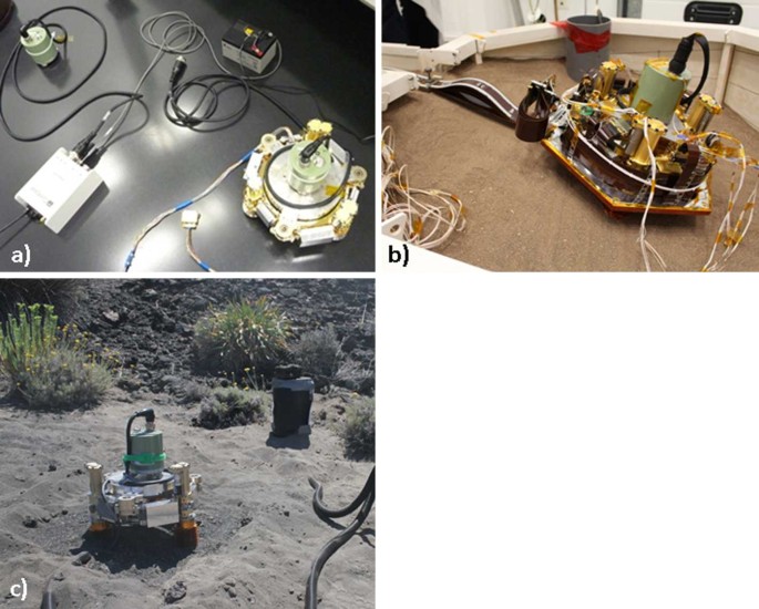
The three configurations for which LVL effects on the Rayleigh wave ellipticity were analysed. a) LVL flight model installed on the floor of the MPS clean room. The green cylindrical instrument on top of the LVL is the Trillium compact sensor. The reference sensor, placed on the ground next to the LVL, is visible in the upper left of the picture. During the measurements, both the reference sensor and the LVL were covered to provide protection from the wind noise produced by the venting in the clean room. b) LVL qualification model in the sandbox at CNES. The reference sensor is directly behind the LVL on the sand and cannot be seen in this picture. A second reference sensor is placed in the grey PVC tube at the back of the sandbox, in direct contact with the ground beneath the sand. The whole sandbox was covered by thermal and wind shielding during the measurements. c) LVL engineering model on Vulcano island. The reference sensor is in the center background beneath the black thermal and wind cover provided by the manufacturer. During the measurements, the LVL was also covered by a thermal and wind protection
-
2.
CNES: A measurement taken with the LVL qualification model in a sandbox in the cleanroom of the Centre National d’Etudes Spatiales (CNES) in Toulouse. The model in this case was more complete, including the bottom plate of the RWEB thermal enclosure and the SEIS tether (Lognonné et al. 2018). The LVL was in a tilted configuration. A reference sensor was placed on the sand next to the LVL, and another one in a PVC tube on the bottom of the sandbox, i.e. not within the sand (Fig. 7b). Data were sampled at 100 Hz and 6 hours of continuous recordings were available for analysis.
-
3.
Vulcano: A measurement taken with the LVL engineering model on Vulcano (Aeolian Islands, Italy) on basaltic sand in a tilted configuration. A reference sensor was placed on a thin rock plate (∼1 cm thick) in the sand next to the LVL (Fig. 7c). Data were sampled at 200 Hz and 6 hours of continuous recordings were available for analysis.

2.5 Extraction of Rayleigh Wave Ellipticity and Identification of Instrumentation Resonances
The conventional H/V measurement, which just considers the ratio between horizontal and vertical spectra, might not provide a true measure of the Rayleigh wave ellipticity as it can be biased by other contributions to the wavefield, i.e. body waves or Love waves. Specifically, the Love wave Airy phase might have a strong influence on H/V curves (Bonnefoy-Claudet et al. 2008). Single-station methods that attempt to extract parts of the ambient vibration wavefield dominated by Rayleigh waves before calculating the spectral ratio are based on the \(\pi /2\) phase shift between the vertical and radial component of Rayleigh waves. Methods tested in the previous study and again applied here are H/V based on time-frequency analysis (HVTFA, Kristekova 2006; Fäh et al. 2009) and the RayDec method (Hobiger et al. 2009). The HVTFA method tries to identify Rayleigh waves by searching for maxima on the vertical component data after transferring them into the time-frequency domain by using a continuous wavelet transform, based on modified Morlet wavelets. Time windows that contain mainly horizontal energy are thus excluded from consideration. The ellipticity is calculated by using the maximum horizontal component value with a \(\pm \pi /2\) phase shift for each vertical maximum, as diagnostic of Rayleigh waves. All values at a given frequency are analysed statistically via filtering of histograms. For the RayDec method, the data are split into short analysis time windows which are shifted by \(\pi /2\) for the horizontal compared to the vertical component. The radial direction of the signal in each time window is obtained by maximizing the correlation between a rotated horizontal component and the vertical component while varying the rotation angle. Radial and vertical components for all time windows are stacked, with the correlations as weighting factors, and divided to obtain the ellipticity value. Thus, both methods try to identify parts of the signal that are dominated by Rayleigh waves, and use only these parts or at least weigh them significantly higher in the analysis. However, it is not self-evident that this will also remove signals generated by resonances of the lander or the LVL.
Possibilities to distinguish between spectral signals generated by the ground response and those caused by industrial sources which might contaminate the H/V curve have been studied previously. For example, sharp peaks in the H/V curve, with sharpness increasing with decreasing smoothing used in the calculation, and low damping at the corresponding frequencies have been proposed as indications of an industrial origin of the H/V peak (SESAME European Research Project 2004). This would mean that the measured peak frequency is unreliable for interpretations in terms of site amplification and characteristics. The term “industrial sources” in this context refers to machines that continuously generate energy at monochromatic frequencies, thus creating a permanent signal independent of the ambient wavefield. This is different from possible installation-related sources for SEIS: they also generate signals with specific frequencies, but lander vibrations are caused by winds that are also expected to be a major source of the ambient noise transmitted through the ground to SEIS, and the resonances of the levelling system are generated in response to the ambient vibration ground motion. Still, these signals are related to the vibrations of mechanical structures, which might exhibit different characteristics, e.g. higher \(Q\), compared to the resonances within the regolith at the landing site. Thus, it is worthwhile to examine them in light of the proposed characteristics of industrial sources and see if these can help to distinguish ellipticity peaks caused by lander or LVL resonances from signals related to the subsurface structure.
The damping of signals within a narrow frequency range, which might indicate their industrial origin, is usually measured with the random decrement technique. This technique was originally developed as a tool to check for impending structural failure in aerospace structures using the ambient wavefield (Cole 1973). It has then also found applications in structural health monitoring and measurement of eigenmodes of other engineering structures, e.g. bridges (e.g. Huang et al. 1999; Rodrigues and Brincker 2005) or buildings (e.g. Mikael et al. 2013). In the context of H/V measurements, it is used to measure the damping of signals by considering the random decrement function as equivalent to the free vibration decay curve (Cole 1973). The underlying assumption is that random vibrations consist of a superposition of a step, impulse and random response, where the step and impulse responses are the solutions for an initial displacement and velocity, respectively. When selecting a large number of time windows with the same initial condition, i.e. signal amplitude, and averaging, the impulse and random responses tend to average to zero, and what remains is the response of the structure to an initial displacement. The method was for example applied to distinguish between a natural versus anthropogenic origin of H/V peaks at different locations by Guillier et al. (2007), who used at threshold value of at least 5% damping to identify H/V peaks caused by the subsurface structure.
2.6 Inversion
Similar to the previous study, we use the conditional Neighbourhood Algorithm (NA, Sambridge 1999; Wathelet 2008) to invert the measured ellipticity curves for subsurface structure. As a direct search method, the NA aims to concentrate sampling in the most promising, i.e. lowest-misfit, regions of the parameter space, with the potential to identify several such regions simultaneously. To further allow for a sufficient sampling of the parameter space, we consider not only one, but five to eight runs of the NA based on different random numbers and initial models for each parameterisation, with more runs for cases with more free parameters, i.e. a larger parameter space to investigate. As in the previous study, we try to find the best model parameterisation by comparing results for several different parameterisations, both in terms of number of layers and in terms of the velocity law in the upper-most layer, by using the corrected Akaike’s information criterion (AICc) for the case of a least-square estimation with normally distributed errors and small sample sizes (Sugiura 1978; Hurvich and Tsai 1989). This criterion combines data misfit with the degree of freedom of the model parameterisation to penalize model complexity that will lead to an increase in variance and over-fitting. It is given by
where \(n_{f}\) signifies the number of observations, here given by the number of samples in the ellipticity curves, \(\hat{e}^{2}\) indicates the sum of estimated residuals for candidate models divided by \(n_{f}\), which is equivalent to the misfit between observed and modelled data in the considered case, and K is the number of free parameters, i.e. the degree of freedom of the model parameterisation. The AICc has been introduced to the inversion of ambient vibration dispersion curves for site characterization by Di Giulio et al. (2012), and been applied to Rayleigh wave ellipticity curves in our previous study (Knapmeyer-Endrun et al. 2017), which also contains a more complete explanation.
We calculate inversion results for model parameterisations with one to five layers over a halfspace, where the upper-most layer can either have a constant velocity or contain a linear or power-law-type velocity increase spread over five sublayers, reflecting the increasing compaction of the sandy regolith with depth. We consider 5000 iterations of each NA run, based on 250 starting models, and add a new model to each of the 100 cells with the lowest misfit in each iteration, resulting in a total of 500,250 models considered per inversion run. The optimum parameterisation is identified by the minimum value of the AICc. We separately consider three different value ranges for the parameters of the regolith layer, as described in Table 1. In the first case, designated “A” in Table 1, the velocity range of the regolith layer is based on laboratory data (Delage et al. 2017) as well as comparison with seismic velocities of the lunar regolith and terrestrial sands (see Morgan et al. 2018, for references and details), and the density is set to the estimated surface value of 1300 kg/m3, i.e. the density increase within the layer is neglected. The range for the regolith thickness is set to 3 to 10 m, to include the minimum and maximum depth of the upper-most sandy layer estimated within the landing ellipse (Warner et al. 2017). Here, as in all cases, the range of velocities and thicknesses of the layers between regolith and half-space are not tightly constrained, as little prior information is available on the elastic properties of coarse ejecta and fractured bed-rock layers. The halfspace velocities and density are selected around those of terrestrial pristine basalt. This parameterisation is similar to the one used in the first constrained inversions in our previous study (Knapmeyer-Endrun et al. 2017) and could be further constrained by incorporating information derived from seismic signals generated by HP3 hammering (Kedar et al. 2017), which are expected to resolve the regolith thickness to within 20% and also provide tighter constraints on the average P-wave velocity of the regolith. In the second set-up, parameterisation “B”, a higher constant value of 1500 kg/m3 is assumed for the density within the regolith, and a value of 2000 kg/m3 instead of 1600 kg/m3 is selected for all subsequent layers. This configuration allows to explore the influence of wrong assumptions on the density structure on the velocity models resulting from the inversion. In additional inversions, using parameterisation “C”, we assume higher velocities in the regolith layer, as used in the previous study (Knapmeyer-Endrun et al. 2017), that lie above 100 m/s for vS and 200 m/s for vP. This value is only reached half-way through the regolith layer, at about 2.5 depth, for vP in the true model. In the previous study, we put increasingly tighter constraints on the regolith velocities (Knapmeyer-Endrun et al. 2017), first based on laboratory measurements, and then also including hypothetic results from the analysis of seismic signals generated by HP3 hammering (Kedar et al. 2017). With this parameterisation, we can investigate the influence of incorrect velocity constraints. We use all of the different parameterisations when inverting the curves derived for the dense compaction, i.e. intermediate, model, but also apply inversions with parameterisation “A” to the medium and very dense compaction models.
3 Results
3.1 Ellipticity Measurement
In the following, we compare H/V and ellipticity curves extracted by different methods from wavefields created by model summation and wavenumber integration, respectively, using the theoretical ellipticity curves of the underlying model as a baseline. When comparing to theory, it has to be considered that none of the techniques is well suited to estimate the true amplitudes in the vicinity of peaks and troughs. For H/V, the amplitudes that should approach infinity and zero are contaminated by wavetypes other than Rayleigh waves and will not be equal to theory for a purely horizontal or vertical Rayleigh wave polarisation. For the methods that try to estimate the ellipticity, on the other hand, the systematic problem is that the correlation between vertical and radial component is used to detect Rayleigh waves. As either the vertical or the radial component vanishes at the peak or trough, the signals are no longer correlated at the corresponding frequencies (Hobiger et al. 2012).
Besides, frequency resolution is limited for each of the measuring techniques, whereas the theoretical curve provides perfect resolution in the frequency domain. In the case of the H/V curve, frequency resolution is limited by spectral smoothing, which statistical analysis by Picozzi et al. (2005) found indispensable to get a stable estimate of average H/V values. Here, we apply spectral smoothing according to Konno and Ohmachi (1998) that uses a constant bandwidth on a logarithmic scale with a smoothing constant of 40. HVTFA as a wavelet-based method has a trade-off between resolution in the frequency and time domain, which is determined by the Morlet wavelet parameter. The absolute values of time and frequency resolution are dependent on the considered frequency. The value of 8 for the wavelet parameter chosen here is based on the recommendation derived by Fäh et al. (2009) who considered the fit between theoretical and measured curves for synthetic seismograms calculated for a set of 13 diverse models. It corresponds to a time resolution of 0.386 s and a frequency resolution of 0.206 Hz around the peak frequency. For RayDec, the frequency resolution is determined by the filter bandwidth used. In the previous study (Knapmeyer-Endrun et al. 2017), we selected an optimum value of 0.1\(f\), with \(f\) being the central frequency of the filter band, by comparing the measured curve with the theoretical one, as exercised by Hobiger et al. (2009) when introducing the method.
3.1.1 Simulation Based on Modal Summation
H/V and ellipticity curves extracted from a synthetic noise wavefield based on modal summation for the intermediate regolith profile (dense compaction) are shown in Fig. 8a–c. The modelling of the wavefield here is the same as in Knapmeyer-Endrun et al. (2017), but the updated structural model (Fig. 1) is used. The different panels allow a comparison between different ellipticity estimates, i.e. the standard H/V curve, the HVTFA, and the RayDec estimate, and also show the forward calculated fundamental and first higher mode Rayleigh wave ellipticity curves for reference. Parameters used in the different methods are comparable to the previous study, with a value of 8 for the Morlet wavelet parameter and the use of 5 maxima per minute for HVTFA. However, for the higher mode curve, we selected 10 maxima per minute as this allowed to follow the curve to lower frequencies with confidence, while the rest of the curve remained unaffected. When applying RayDec, we use a time window length of 10/\(f\), and a bandwidth of 0.1\(f\), with \(f\) being the central frequency of the respective filter band.

Comparison of ellipticity curves resulting from the application of different methods to the synthetics based on modal summation and wavenumber integration. Black and grey line in each plot indicate the theoretical fundamental mode and first higher mode Rayleigh wave ellipticity curve, respectively. a) Standard H/V curve with standard deviation (light blue) for the wavefield modelled by modal summation (Fig. 3a). b) HVTFA result with standard deviation (light green) for wavefield modelled by modal summation, including fundamental and first higher mode curve. Dots indicate the part of the curve that would be used as inversion input. c) RAyDec results for wavefield modelled by modal summation with standard deviation (orange) calculating from averaging over results for five minute long time windows. d) Same as a) for wavefield based on wavenumber integration (Fig. 3b). e) Same as b) for wavefield based on wavenumber integration. f) Same as c) for wavefield based on wavenumber integration
All measured curves show similar peak frequencies around 7 Hz and are unable to resolve the true peak amplitudes as well as the detailed structure, i.e. the two maxima the peak is composed of. Furthermore, all methods tend to overestimate the ellipticity amplitude at low frequencies. All methods provide a good estimate of the right flank of the fundamental mode curve. However, at frequencies above 11 Hz, the standard H/V and RayDec curves deviate from the true ellipticity amplitudes due to an overlap between the fundamental and first higher mode in the synthetic wavefield which cannot be resolved by these two techniques. In fact, the RayDec curves provides a good approximation of the first higher mode Rayleigh wave ellipticity at high frequencies. The HVTFA curve, on the other hand, allows to resolve both curves independently. However, compared to the baseline model in the previous study, the first higher mode cannot be followed to lower frequencies, i.e. the left flank of its minimum. There are slight differences in the quality of the estimate of the left flank of the fundamental mode peak. The standard H/V method tends to overestimate the ellipticity values. RayDec results are closer to theory, but still contain some overestimation, whereas the HVTFA results are closest to the theoretical curve, also at frequencies between 3.5 and 5 Hz, i.e. at the transition from the peak to constant ellipticity values at low frequencies.
3.1.2 Including Body Waves
Results for the modelling that is explicitly based on body waves by building up the wavefield by wavenumber integration are not markedly different. The left flank of the fundamental mode ellipticity peak is slightly closer to the true value for all methods of estimation, and the value of the curve at low frequencies appears better constrained, i.e. is closer to 1 than to 2, in all cases. When applying HVTFA to the wavenumber integration data set and using a low number of peaks per minute, i.e. 2 or less, the left flank of the fundamental mode ellipticity peak is harder to discern than for the synthetics based on modal summation, indicating that less surface wave energy is present in the wavefield. A longer measurement time might be needed in this case to better constrain the curve at long periods.
Ellipticity curves derived by HVTFA for the three different models with varying compaction in the regolith are compared in Fig. 9. Differences comparable to those observed in the forward modelled curves (Fig. 2) are visible, with the curves with lesser compaction, i.e. lower densities in the regolith layer, shifted to slightly lower frequencies compared to the curves with a higher compaction. The shift affects both flanks of the fundamental mode ellipticity peak as well as the measurable part of the first higher modes. At least with synthetic data, the difference between the three models is indeed measurable. However, the differences are rather small, so it is investigated in the next section how much they might influence the inversion results when attributed to changes in velocity and not density.

Ellipticity curves derived by HVTFA from wavenumber integration synthetics for the three models under consideration. Colour coding is the same as in Fig. 2, i.e. red, black, and blue colours refer to models with medium, dense, and very dense regolith compaction
3.2 Instrumentation Resonances
3.2.1 Lander Mechanical Noise
Two approaches are used to understand the effect of lander mechanical noise on ellipticity measurements with SEIS. The first is based on the flexible mode model of the lander presented by Murdoch et al. (2018), the second one on field observations.
The flexible mode model describes the response of the lander structure to an external force, i.e. the aerodynamic load due to winds, in terms of the forces exerted at the coupling points with the ground. As the lander structure and the ground are modelled as a coupled oscillating system, the response of the system depends on both the characteristics of the wind force and the properties of the ground, specifically the ground stiffness and damping under the lander feet (Murdoch et al. 2018). To estimate the amplitude and frequency of seismic signals recorded by SEIS due to lander vibrations, the modelling further calculates the ground deformation at the base of the SEIS LVL in the baseline deployment configuration by using an elastic ground deformation model (Murdoch et al. 2017). This model considers the ground as an elastic half space with properties of the Martian regolith and determines the deformation of this elastic medium in response to forces applied to its free surface by using the Boussinesq point load solution (Boussinesq 1885). Further details are provided by Murdoch et al. (2018).
This dynamic model contains two contributions to the high-frequency lander noise. One are the flexible modes of the lander itself, the other consists of induced reverberations of the solar panels. Only the first contribution can be studied in a realistic manner with the model at hand due to limited available information on the solar panels. The resonant frequencies of the lander flexible modes depend on the ground stiffness and increase logarithmically with increasing stiffness (Murdoch et al. 2018). In Fig. 10, we compare these frequencies and their variation with ground stiffness, realised by changing only the P- and S-wave velocities beneath the lander, as in Murdoch et al. (2018), with the corresponding frequency of the fundamental mode Rayleigh wave ellipticity peak. As the parameters used by Murdoch et al. (2018) correspond to the medium regolith compaction model (Morgan et al. 2018), we also use this model here. Synthetic ellipticity curves are calculated for the different surface velocities corresponding to the stiffness values, while using the same relation for the velocity increase with depth within the regolith as in Morgan et al. (2018) and Delage et al. (2017). As a thinner regolith layer with the same velocities will lead to an ellipticity peak at a higher frequency, we additionally consider a regolith thickness of 3 m, the minimum value reached in 85% of the landing ellipse. For both cases, and all ground stiffness values analysed here, the Rayleigh wave ellipticity peaks are clearly separated in frequency from the lander resonant modes. The difference between the ellipticity peak and the lowest of the lander flexible modes is at least 10 Hz for the thin regolith layer, and more than 15 Hz for the baseline model. Thus, no overlap between the different signals is expected.

Comparison of lander resonant frequencies derived from flexible mode modelling and Rayleigh wave ellipticity peak frequency in dependence on ground stiffness. Each of the blue and green lines corresponds to the peak frequencies of one of the six different resonant modes of the lander (Murdoch et al. 2018). The red curve gives fundamental mode ellipticity peak frequencies for the medium compacted model with 5 m regolith thickness, whereas the orange line corresponds to peak frequencies for a reduced regolith thickness of 3 m
The solar panel resonances occur between 8.5 and 12 Hz in the baseline model and these resonant frequencies do not change with ground stiffness, as they are dictated solely by the mechanics of the attachment points to the lander (Murdoch et al. 2018). This means there could be some overlap in frequency between the solar panel resonances and the structural response of the ground, if the amplitudes of these resonances are large enough to make them resolvable. The amplitude of the resonances observed by SEIS increases with decreasing seismic velocities, for both the lander flexible modes and the solar panel vibrations, but additionally depends on the wind amplitude and direction. For the baseline model, the amplitudes are below the instruments’ self noise, but for seismic velocities 50% smaller than in the baseline model, the amplitudes of the lander flexible modes could actually be larger than the self noise. The amplitudes of the solar panel resonances are an order of magnitude smaller in this modelling, though, and still below the self noise. This might however be related to the specific set-up of the model that does not allow for a direct interaction between the solar panels and the wind.
The horizontal-to-vertical spectral amplitude ratio for the lander resonance with the highest amplitudes, which also has the lowest frequencies, is around 4. The spectral amplitude ratio of the solar panel vibrations at the lowest frequencies is around 5, and 2 at higher frequencies, for the baseline model. Depending on the Rayleigh wave content in the lander and solar panel resonances, and how well they could be separated from other components of the wavefield by HVTFA, the actual measured ellipticities might be smaller than the maximum estimates given here. The spectral ratio of the solar panel reverberations increases with decreasing ground velocities, but also depends strongly on the vertical angle of attack of the wind. A larger angle of attack strongly increases the lift and drag force contribution in the interaction between lander and wind and this, in turns, increases the signal on the vertical axis. For vertical angles of attack of 10o and larger, the vertical spectral amplitudes of the solar panel vibrations are actually larger than the horizontal ones, so that the spectral ratio would be less than one (Murdoch et al. 2018).
More information on the visibility and amplitudes of lander and solar panel resonances in seismograms recorded close to the lander might be gained from the field experiment at Mt. Etna. We analyse data for the three different configuration (no lander, lander with solar panels closed, and lander with solar panels open) for a variety of different wind levels. Generally, we analyse three to four hours of data recorded during the night time, i.e. with little human activity, during which the wind velocity as averaged over 30 min time intervals showed little variation (Table 2). The one exception are data with open solar panels, as the panels were only opened manually during daytime when the field team was at the site and the wind level was deemed sufficiently low. However, the level of human activity, including hammering for an active seismic experiment and driving a rover to demonstrate the deployment of a remote unit picked up at the lander, increased significantly during that time. Hence, we could only analyse shorter time windows of one hour length when there was a break in these activities.
The spectra of the seismic data before the lander was deployed are very similar at frequencies below about 10–15 Hz, but show a strong dependence on the wind strength above, with increasing amplitudes for increasing wind velocities (Fig. 11a–c). For the lowest frequencies considered, between 1 and 3 Hz, there also seems to be an influence of wind strength on the relative distribution of energy between the two horizontal components, with more energy on the North and less energy on the East component for higher winds. This observation could however also depend on other factors, e.g. changes in the dominant wind direction, and further analysis is beyond the scope of this paper. Additionally, all spectra show a bump between 40 and 50 Hz that becomes more prominent for higher winds. After the deployment of the lander at about 10 m distance from the station, variations occur in the wind-related part of the spectrum, whereas the spectral shape at frequencies below 10–15 Hz remains basically unchanged (Fig. 11d–f). The bump between 40 and 50 Hz has vanished, even for the lowest wind velocities, whereas the general shape of the vertical spectrum at high frequencies above 40 Hz looks much flatter than before. With increasing wind velocity, another peak around 25 Hz appears, first, i.e. already at average velocities of 4.2 m/s, on the vertical component, but for velocities of 8.1 m/s and higher also on the horizontal components. The peak’s frequency is also within the range of the frequencies of the lowest, and largest, flexible mode of the InSight lander calculated for a low ground stiffness (Fig. 10). The shape of the horizontal component spectra looks different, too, with amplitudes significantly higher between 10 and 50 Hz for comparable wind speeds around 4 m/s. With the solar panels extended, no clear additional signals occur, but the spectral peak around 25 Hz is visible on the vertical component for average wind velocities of both 2.7 m/s and 8.3 m/s, and the amplitude increase on the horizontal components is also apparent (Fig. 11g–h).

Power density spectra for measurements on Mt. Etna to characterize lander and wind effects. Different colours refer to measurements taken during different average wind velocities, as given in the legend. a) North component for measurements before the lander mock-up was installed next to the sensor. b) East component for measurements before the lander mock-up was installed next to the sensor. c) Vertical component for measurements before the lander mock-up was installed next to the sensor. d) Same as a) with lander mock-up, but solar panels closed. e) Same as b) with lander mock-up, but solar panels closed. f) Same as c) with lander mock-up, but solar panels closed. g) Same as a) with lander mock-up and all four solar panels open. h) Same as b) with lander mock-up and all four solar panels above. i) Same as c) with lander mock-up and all four solar panels open
Considering the H/V curves, the most prominent and consistent signal is the peak around 0.8 Hz (Fig. 12). It shows some similarity to the InSight synthetics in that it seems to consist of two overlapping peaks. The frequency of the higher-frequency peak shows a close correspondence to the estimated resonance frequency of the top-most sand layer at 1.15 Hz, based on results from refraction profiling at the site. Estimated P-wave velocities below this layer are still below 300 m/s and indicate sediments, whereas a lava flow is expected at larger depth. This could explain the double peak in the H/V curve. Without the lander deployed, the high-frequency part of the curve shows another broad peak between 10 and 20 Hz, where the position of the upper flank seems to be strongly wind-dependent, though (Fig. 12a). This effect seems only to increase when HVTFA is applied. The spectral bump between 40 and 50 Hz does not have a clear H/V signature. The main change to the H/V curve once the lander is deployed is a strong minimum around 25 Hz, the amplitude of which is wind-dependent (Fig. 12c). The broad peak between 10 and 20 Hz is now also stable and independent of the wind, and HVTFA brings out an additional narrow peak around 30 Hz, once the wind is above the threshold for lander influence. These features are the same when the solar panels are open (Fig. 12e, f); no indication of any clear solar panel resonances is apparent in the H/V and HVTFA curves.

H/V spectral ratios and estimated Rayleigh wave ellipticity for data collected at Mt. Etna. Colour coding is the same as in Fig. 11 and related to average wind velocity. a) H/V spectral ratios measured without the lander placed in the vicinity of the seismometer. b) Rayleigh wave ellipticity estimated using HVTFA for the same data as in a). c) Same as a) with lander emplaced, but solar panels closed. d) Same as b) with lander emplaced, but solar panels closed. e) Same as a) with lander in place near the seismometer and all four solar panels open. f) Same as b) with lander in place near the seismometer and all four solar panels open
We use the random decrement technique to estimate the damping of the free oscillation response at different frequencies for two of the analysed time windows, namely the one with open solar panels and low winds on 06/25, and the one with closed solar panels and high winds on 06/27 (Table 2). We considered frequency ranges around the spectral peak that we associate with the lander (around 25 Hz) and that is accompanied by a minimum in the H/V and ellipticity curves, and the peak likely associated with sub-surface structure (around 1 Hz). For both time windows, the frequency range associated with lander resonances exhibits low damping ratios around 1.1% to 1.3%, whereas the frequencies around the suspected structural response show significantly higher damping ratios between 5.3% and 6.7% (Fig. 13). In both frequency ranges, the estimated damping ratio is higher during the time window with lower winds.

Random decrement signatures of signals recorded at Mt. Etna to estimate damping. Black, solid line is the average curve with dashed lines giving the standard deviation. Red line is the fit to the curve by an exponentially decreasing sine function. a) East component data recorded on 06/25 with open solar panels, filtered between 0.9 and 1.35 Hz. Damping ratio of the fitted curve is 5.87%, average value for all three components is 6.66%. b) Vertical component data recorded on 06/25 with open solar panels, covering the frequency range between 24 and 28 Hz affected by lander noise. Damping ratio of the fitted curve is 1.30%, average value for all three components is 1.27%. c) North component data recorded on 06/27 with closed solar panels, filtered between 0.9 and 1.35 Hz. Damping ratio of the fitted curve is 5.22%, average value for all three components is 5.30%. b) Vertical component data recorded on 06/27 with closed solar panels, covering the frequency range between 24 and 28 Hz affected by lander noise. Damping ratio of the fitted curve is 1.04%, average value for all three components is 1.08%
3.2.2 LVL Effects
Possible LVL effects are studied by considering the three measurement setups discussed in Sect. 2.2. The spectral peaks caused by the LVL resonances show up clearly on the horizontal spectra in all considered cases at frequencies between 35 and 45 Hz (Fig. 14), even though the spectra from the lab measurements contain a lot of additional narrow, high-frequency peaks likely related to machinery in the building, including the venting of the clean room, the power grid at 50 Hz, and multiples. These peaks are clearly sharper than the one caused by the LVL. The comparison to the reference sensor(s) provides a baseline to identify the LVL effect in these measurements; however, it has been demonstrated that estimates of the peak frequency solely based on power density spectra of the sensor on the LVL, as compared to transfer function estimates between the reference sensor and the sensor on the LVL, show negligible differences (Fayon et al. 2018).

Power density spectra for measurements to characterize the LVL effect. In each plot, the red curve represents data from the seismometer on the LVL, whereas the blue curve represents data from the reference sensor next to the LVL. For the CNES measurements (d–f), the green curves are data from the reference sensor placed in a PVC tube without sand. a) Horizontal X-component for measurement on the floor in the MPS cleanroom. b) Horizontal Y-component for measurement in the MPS cleanroom. c) Vertical component for measurement in the MPS cleanroom. d) Same as a) for measurement in sandbox at CNES. e) Same as b) for measurement in sandbox at CNES. f) Same as c) for measurement in sandbox at CNES. g) Same as a) for measurement on volcanic sand on Vulcano island. h) Same as b) for measurement on Vulcano island. i) Same as c) for measurement on Vulcano island
In case of the measurements done at CNES, a prominent, broad frequency peak around 25 Hz shows up on all three components of both reference sensors as well as of the sensor on the LVL. Less clear peaks occur around 10 Hz for the MPS measurements and 20 Hz for the Vulcano measurements. No indication of resonances between the LVL and the regolith at high frequencies that affect the vertical component only, as observed by Myhill et al. (2018) during a field campaign in Iceland, are evident for the two cases in which measurements were conducted on sand. Spectral peaks observed on the vertical component are matched closely on the horizontal ones, as described above, and are also visible on the reference sensor. However, at lower frequencies, higher amplitudes on the vertical compared to the horizontal components are observed for the measurements on sand, i.e. for all sensors around 2 Hz in the CNES case and, less clear, around 1.6 Hz for the measurement on Vulcano. These frequencies are smaller by an order of magnitude than predicted by Myhill et al. (2018), and the exactly same effect is also observed on the reference sensors not mounted on the LVL, and, in case of the CNES measurements, not placed on sand, so it is hard to link the amplitude increase to the LVL. Compared to the study by Myhill et al. (2018), the reference sensor was not buried here, so it might see some of the same free-surface effects as the sensor on the LVL. An exception is the case of the sensor placed in the PVC tube during the CNES measurements that is not in direct contact with the sand at all. It might however still have been affected by coupling of sand resonances to the tube and the tube’s contact to the boundary of the sand box. Further differences to the study by Myhill et al. (2018) include their use of a close, mono-frequent, active source, more comparable to the lander or HP3 hammering signals than to the ambient vibration wavefield, and of a rigid tripod of different dimensions, shape, and material than the LVL.
Concerning the H/V curves, the most prominent peak is that related to the LVL resonances in each case (Fig. 15). Application of HVTFA does little to dampen this peak, i.e. it is not filtered out by application of the \(\pi /2\) phase shift criterion to isolate Rayleigh waves. With the exception of the LVL peak, amplitudes never rise above 2 for frequencies above 1 Hz for deployments on sand. The Vulcano measurements show a clear peak around 0.33 Hz (Fig. 15e, f). This frequency seems rather low for a signal related to the sand layer, though information on the detailed subsurface structure of the site is missing. The peak might instead be related to the influence of the local environment, i.e. a near-by cliff dropping several meters to the sea. In case of the measurement in the MPS lab, a broad peak between 2 and 4 Hz is observed (Fig. 15a, b). As this measurement took place on the ground floor of a building, the peak could be associated with building resonances rather than a subsurface response. The CNES data show a prominent minimum in the H/V curve around 20 Hz which has the lowest amplitudes, by about a factor of two, for the sensor on the LVL (Fig. 15c, d). This minimum is related a decrease in spectral amplitudes on the horizontal components relative to neighbouring frequencies and to the vertical component at all three sensors. However, the vertical component shows the largest amplitudes for the sensor on the LVL, so the H/V minimum is most pronounced here. As the H/V minimum is related to a signal decrease on the horizontal components rather than an increase on the vertical component, it cannot be linked to vertical resonances (Myhill et al. 2018), and might rather be related to a dominantly vertical polarization of Rayleigh waves.

a) Standard H/V curves derived from measurements in the MPS cleanroom. Colour coding is the same as in Fig. 14. b) Red curve is the H/V curve derived from the sensor on the LVL as shown in a), grey curve is the result of HVTFA applied to this data set, with uncertainty. c) Same as a) for measurement in sandbox at CNES. d) Same as b) for measurement in sandbox at CNES. e) Same as a) for measurement on Vulcano island. f) Same as b) for measurement on Vulcano island
We applied the random decrement technique to the data measured in the MPS clean room and on Vulcano, respectively, and compared the random decrement signatures in terms of damping ratio around the frequency of the LVL resonances and the other maxima described above (Fig. 16). In both cases, all estimated damping ratios are rather low. For the data acquired in the MPS clean room, the damping ratio around the LVL resonance frequency is about 0.5% for the horizontal components, and four times as large, around 2%, at frequencies between 3.2 and 4.0 Hz. The data from Vulcano show a somewhat higher damping ratio for the LVL resonances, about 1% on the horizontal components, but the damping of the peak around 0.33 Hz is still three times larger, at around 3%. The vertical component shows larger damping ratios (1.1% and 1.4%, respectively) in the frequency range of the LVL resonance, but as the vertical spectra are not influenced by the resonance, we consider the horizontal components to be the significant ones here.

Random decrement signatures of horizontal component signals recorded on the LVL to estimate damping. Black, solid line is the average curve with dashed lines giving the standard deviation. Red line is the fit to the curve by an exponentially decreasing sine function. a) Data from the MPS clean room, filtered between 3.2 to 4.0 Hz. Damping ratio of the fitted curve is 2.09%, average value for all three components is 2.03%. b) Data from the MPS clean room, covering the frequency range between 43 and 47 Hz (LVL resonance). Damping ratio of the fitted curve is 0.47%, average value for the two horizontal components is 0.50%. c) Data measured on Vulcano island, filtered between 0.28 and 0.38 Hz. Damping ratio of the fitted curve is 2.92%, average value for all three components is 3.00%. d) Data measured on Vulcano island, considering frequencies between 38 and 43 Hz (LVL resonance). Damping ratio of the fitted curve is 1.05%, average value for the two horizontal components is 1.04%
3.3 Inversion
For the dense compaction model used as a baseline here, application of the AICc to inversion results for parameterisation “A” (Table 1) indicates that the best model parameterisation consists of two layers over a halfspace, with a power-law velocity increase in the upper-most layer. The same type of optimum parameterisation was obtained in the previous study for a model with a larger regolith thickness and higher regolith velocities (Knapmeyer-Endrun et al. 2017). The optimum parameterisation is the same, regardless of whether only the fundamental mode curve or both the fundamental and higher mode curves are inverted. The inversion results (Fig. 17) provide a good estimate of the thickness of the sandy regolith layer in both cases. When inverting the fundamental mode only, the estimated depth range of the regolith layer is 3–5.6 m. Including the higher mode tightens these constraints to 4.9–5.7 m, and also provides a very close match to the actual velocities in the regolith layer. The deeper structure is not as well resolved, though. Velocities of the coarse ejecta layer tend to be over-estimated, and S-wave velocities are only resolved to be larger than 600 m/s and 850 m/s in the fundamental mode and fundamental and higher mode case, respectively. The depth extent of the coarse ejecta layer is constrained to between 10 and 30 m in both cases, bracketing the fractured basalt layer with its gradually increasing velocities. The velocity of the bottom, basalt layer is not constrained at all; models that can explain the data cover the whole investigated parameter range.

Velocity models and fit to the data for the best parameterisation, corresponding to the minimum AICc, for the baseline model using model parameterisation “A” (Table 1). a) Inverting the fundamental mode ellipticity curve only, b) inverting both fundamental and higher mode. Black lines outline the boundaries of the parameter space investigated in the inversion. Central black line is the true model. Red line indicates the best-fitting model found. For the ellipticity curves, black dots with error bars outline the measured data. Red dashed lines are the theoretical curves for the best-fitting model. The colour scale is the same in all subplots. In both cases, all models with a misfit below 0.61 are judged to satisfy the data
When using parameterisation “B”, with higher densities in the top and intermediate layers (Table 1), the inversion results are virtually identical. The same best parameterisation is obtained, and the same depth and velocity ranges are covered by models that can explain the data within their uncertainties. The best model is identical when only the fundamental mode is inverted and nearly identical, with slightly higher velocities and a corresponding larger thickness for the second layer for parameterisation “B”, when the higher mode data is included.
According to the AICc, the optimum model parameterisation when inverting the synthetics calculated for the intermediate and very dense regolith compaction models with parameterisation “A” (Table 1) consists again of two layers over a half-space, with a power-law type velocity increase in the first layer, for both inversions of the fundamental mode only and of the fundamental and higher mode. The range of acceptable models is very similar to that for the dense compaction baseline model, especially when only the fundamental mode is considered. The clearest difference is observed when both fundamental and higher mode are inverted for the very dense compaction model. Here, the obtained velocities in the second layer are higher, above 1000 m/s for S-wave and 1600 m/s for P-waves, and the layer extends to a minimum depth of 13 instead of 10 m (Fig. 18). No corresponding differences are observed in the results for the intermediate compaction model. Inverting the fundamental and higher mode data from the very dense regolith compaction model with parameterisation “B”, i.e. using higher fixed densities in the top and intermediate layers, gives results that are in good agreement with the velocities obtained when inverting the baseline model, though (Fig. 18).

Velocity models and fit to the data for the best parameterisation, corresponding to the minimum AICc, for synthetics based on the very high compaction model. a) Using model parameterisation “A”, b) using model parameterisation “B”. Model space and data are drawn as in Fig. 17. The colour scale is different in a) and b), and models with a misfit below 0.83 and 0.82 are judged to satisfy the data
The picture changes when parameterisation “C”, assuming higher velocities in the upper-most sandy regolith layer, is used. In this case, the optimum model parameterisation consists of three instead of two layers over a halfspace for the baseline model (Fig. 19). Here, the thickness of the topmost regolith layer is at the upper boundary of the parameter space, at only 3 m. However, the velocity contrast to the subsequent layer is rather small, with velocities in this layer also at the lower bound of the parameter space, i.e. around 300 m/s and 500 m/s for S-waves and P-waves, respectively. This second layer is extending to 9 to 16 m and 9 to 12 m depth for the fundamental mode and the fundamental and higher mode case, respectively. The transition to the bottom layer is found between 14 and 26 m and 15 and 25 m depth, respectively. From the surface to a depth of 11 to 16 m, the true model lies outside the range of inverted models that can explain the data.

Velocity models and fit to the data for the best parameterisation, corresponding to the minimum AICc, for the baseline model using model parameterisation “C” (Table 1). a) Inverting the fundamental mode ellipticity curve only, b) inverting both fundamental and higher mode. Model space and data are drawn as in Fig. 17. The colour scale is the same in all subplots. In both cases, all models with a misfit below 0.51 are judged to satisfy the data
4 Discussion
4.1 Synthetic Wavefield Modelling and Scaling
Ellipticity calculations for the updated regolith model of the landing site, with a more realistic regolith thickness of 5 m, indicate that amplification of horizontal signals due to structural resonances can be expected between about 6 and 9 Hz. This is above the nominal data rate for both the continuous VBB channels at 2 Hz and the VELZ channel at 10 Hz; the later will in general not contain horizontal data. However, the resonances would affect both full rate VBB and SP data, sampled at 20 Hz and 100 Hz, respectively. The frequency range affected would likely not be of interest for the interpretation of teleseismic data, but might be used for regional and local events. If the regolith thickness is closer to the estimated minimum, i.e. 3 m, the influence on the VBB data would be reduced as the structural resonance would be located around 10 Hz.
Our order-of-magnitude amplitude scaling of the synthetic noise wavefield indicates that the amplitudes of seismic noise generated by the atmosphere (e.g. dust devils) should be above the self-noise of SEIS even if sources are not within the immediate vicinity of the station, especially when stacking a sufficiently large amount of data. Based on this scaling, the amplitude of the background wavefield is also an order of magnitude larger than the amplitude of the largest lander flexible mode resonance for the baseline model, so these resonances would only constitute a minor contribution. We did not consider variations in \(Q\) when transferring the amplitudes of the terrestrial recordings from the Mojave desert to Mars. \(Q\) in the regolith model is higher than commonly observed for sands on Earth, meaning that terrestrial data should contain more attenuation. However, Myhill et al. (2018) observed a larger attenuation than predicted by elastic theory for seismic signals generated by a spring source on volcanic sand in Iceland, which they attribute to enhanced dissipation of energy by grain sliding in unconsolidated regolith. This effect could potentially reduce the amplitude of atmospheric signals transmitted through the Martian regolith to SEIS. In granular material, attenuation will also depend on the size of the displacement, with \(Q\) inversely proportional to the strain amplitude (Brunet et al. 2008). Larger displacements would thus see a lower \(Q\), i.e. higher damping, which could be important when making inferences about the ambient background wavefield based on measurement with a near, active source. Another point that is not considered in the modelling is the possible complexity of atmospheric sources, e.g. movement of dust devils towards and away from the station. This aspect, together with a more precise amplitude scaling, could be incorporated in modelling that couples large eddy simulations of the Martian atmosphere with seismic wave propagation in the shallow subsurface. This approach would be computationally more expensive, though, and is left for future work.
The simulated wavefields are broadly similar, regardless of whether the faster modal summation approach, building up the wavefield from surface waves, or the slower wavenumber integration approach, building up the wavefield from body waves, is used. The extracted ellipticity curves also show a high similarity and are close to the theoretical curves. These results increase the confidence that the ellipticity information will also be recoverable from actual Martian data with unknown relative contributions of body and surface waves. In the previous study, the first higher Rayleigh mode was prominently visible in the H/V and ellipticity curves (Knapmeyer-Endrun et al. 2017). Indeed, the dominant influence of higher modes in an ambient noise wavefield at shorter periods and its influence on measured H/V ratios was observed in actual ambient vibration data from Christchurch, New Zealand (Savage et al. 2013). Though the synthetic wavefield simulated here should generate higher mode Rayleigh wave energy to the same extent as the one used in the previous study, specifically for the modal summation case, the observed first higher mode is much weaker and limited to higher frequencies, i.e. part of the right flank of the minimum and beyond. This can be understood by considering the influence of \(Q\) on the different modes. At a given frequency \(f\), the first higher mode has a higher phase velocity c than the fundamental mode. This, in turns, means that the wavelength \(\lambda \) of the higher mode also has to be larger, as \(c=f\lambda \). For a given propagation distance, the fundamental mode will thus have more propagation cycles, and will be stronger affected by damping, than the higher mode. As \(Q\) of the current subsurface models is significantly higher, and thus damping lower, than in the baseline model of the previous study, the fundamental mode can propagate over larger distances before being completely attenuated. Accordingly, the good visibility of the higher mode over a broad frequency range in the previous study can be explained by a stronger attenuation of the fundamental mode due to lower \(Q\). As \(Q\) is higher in the current models, the effect is only apparent at high frequencies, where wavelengths are smallest and hence the effect of damping strongest.
4.2 Inversion
The different regolith compaction models have a minor, though detectable, effect on the ellipticity curves. The effect of different densities will be harder to resolve with actual data, which might show larger standard deviations than the synthetics, though. The inversion results indicate a limited influence of the assumptions on density. When incorrect, higher densities are assumed (parameterisation “B”, Table 1), the inversion result is not affected for the baseline model, at least not considering the large range of acceptable models. The variations in the best-fitting model are within the usual depth-velocity trade-off of ellipticity curves (e.g. Knapmeyer-Endrun et al. 2017). The inversion results obtained for the curves derived from synthetics for the intermediate and very dense regolith compaction model are also within the uncertainty range of the results for the baseline model. However, the results for the very dense compaction model and parameterisation “A” (too low densities in the regolith layer) tend to slightly larger thicknesses of the second layer and accompanying higher velocities, if higher mode data are included in the inversion (Fig. 18). In contrast, no prominent effect of different assumed densities is observed when only the fundamental mode data are available. It might therefore be useful to compare results with lower and higher assumed regolith densities, even though the uncertainty of the curves, the trade-offs between different parameters, and the resulting uncertainty in the models are generally large enough to include and mask all density effects.
The velocity range allowed for the upper-most layer has a strong influence on the inversion results, with the faster parameter range “C” leading to a completely different set of models, which does not contain the true model, for the upper 10 m. The well-known depth-velocity trade-off for ellipticity curves (e.g. Knapmeyer-Endrun et al. 2017, Fig. 10) leads to models with a larger thickness of the lowest-velocity layer (comprised of layers 1 and 2) in this case (Fig. 19). The modelled curves in this case contain only a single peak around 7.5 Hz, but can fit the inverted data along the flanks equally well as the two-peaked models for the standard parameterisation “A”. If the data from Mars contain some indication of a double-peaked structure, like in the case of the data from Mt. Etna (Fig. 12) or the HVTFA curve of the synthetics (Fig. 8e), this additional information could be used to discard results that show only a single peak, even if the curve around the peaks itself cannot be picked in detail and used in the inversion. Information on the maximum penetration depth reached by HP3 could in addition be useful to constrain the minimum regolith thickness, i.e. to exclude the models with an only 3 m thick regolith found as optimum solution here (see results for parameterisations using various constraints on regolith thickness and velocity in our previous study, Knapmeyer-Endrun et al. 2017). As the constraints imposed on the upper-most layer have a large influence on the retrieved velocity models, it would be desirable that velocity constraints for this layer are not only based on assumptions derived from laboratory or lunar data. Rather, they should also take into account other experimental results for the actual landing site, e.g. from the interpretation of the seismic data generated by HP3 hammering both in terms of reflection seismic (Kedar et al. 2017) and in terms of wavefield gradiometry with the six individual instruments of SEIS (Fayon et al. 2018).
While the inversion results in general indicate that the constraints used on the velocity of the upper-most layer help to tightly constrain its thickness by resolving the depth-velocity trade-off, the properties of the following layer are less well constrained. The observed over-estimation of velocities is similar to an observation in Knapmeyer-Endrun et al. (2017) for a case with a broad, two-peaked ellipticity maximum. It might partly be attributed to missing data and the resulting large uncertainty around the ellipticity peak. However, considering ellipticity curves for variable velocities of the second layer, up to an increase or decrease by 50%, also indicates that the upper boundary of velocities within this layer will in general be less well constrained than the lower one (Fig. 20). While a velocity decrease by 20% to 50% has a distinct effect, especially on the lower flank of the curve, curves for models with velocities increased by an equal amount plot almost on top of one another. This can explain why the true velocity and thickness of the second layer are always at the lower end of the parameter range that can explain the data. The additional trade-off between layer thickness and velocity within the layer is not considered here, but will not influence the point that decreasing velocities in the second layer have a stronger effect on the shape of the ellipticity curve than increasing ones. The gradual, final velocity increase to the high basaltic velocities is in each case bracketed by the models. It cannot be fit in detail by a parameterisation that allows only constant layer velocities for all but the top-most layer.

Influence of increasing or decreasing the velocities within a single layer on the ellipticity curve. a) Fundamental mode ellipticity curves when the velocities in the uppermost layer of sandy regolith are increased or decreased up to 50% in 10% increments. Velocity decreases are marked by colours from green towards the red end of the spectrum, while velocity increases are indicated by colours from green towards the violet end of the spectrum. b) Same as a) for velocity changes within the second (coarse ejecta) layer of the model
If parts of the ambient vibration background noise are below the self noise of the sensors and the ellipticity curve could be retrieved reliably only within the frequency range between 5.5 Hz and 18 Hz, inversion results are yet again different when considering fundamental mode data only (Fig. 21). The optimum parameterisation in this case consists of three uniform layers, and the velocities in the uppermost 10 m are far from the true model. Results are similar to the ones with the full curve when the higher mode is also considered. This can be explained by the unequal sampling of the left and right flank of the ellipticity peak. When the whole curve is considered, the number of samples on both flanks is equal, but when data below 5.5. Hz are discarded, the number of samples on the left flank that also constrains velocities below the uppermost-layer (Fig. 20) is drastically reduced. In fact, the fit of the best model to the data on the left flank is rather poor (Fig. 21a). This improves when higher mode information is included (Fig. 21b). However, if only a limited frequency range for the left flank is available in the actual data, it could be useful to increase the weight for this part of the curve in the inversion or interpolate the data to a higher number of samples to avoid preferentially fitting only the right flank.

Velocity models and fit to the data for the best parameterisation, corresponding to the minimum AICc, for the baseline model using only data between 5.5 and 18 Hz and model parameterisation “A” (Table 1). a) Inverting the fundamental mode ellipticity curve only, b) inverting both fundamental and higher mode. Model space and data are drawn as in Fig. 17. The colour scale is different in a) and b), and models with a misfit below 0.53 and 0.65 are judged to satisfy the data
4.3 Instrumentation Resonances
In data measured on Mt. Etna under a variety of wind conditions, no influence of the wind velocity on the structural response is observed. The wind only influences the spectra at high frequencies, above about 20 Hz. This is also encouraging for InSight as the structural response of the regolith is expected well below this frequency and should thus remain unaffected by changing wind conditions.
In terms of instrumentation noise, both the LVL resonances and the lander flexible modes occur at significantly higher frequencies than the expected structural signal and are therefore clearly separable from it. It will depend on the elastic ground properties at the landing site if the lander modes are even observable above the instrument self noise. No lander resonances were observed in the Viking 2 seismic data recorded on the lander deck, but the design of the lander was also such that the lander resonances were outside the useful frequency band of the seismometer, considered to extend to 10 Hz (Anderson et al. 1977). The Viking landers did not have any solar panels, which show resonant modes at lower frequencies, as their power was provided by radioisotope thermoelectric generators. The SP sensor is expected to provide useful data to significantly higher frequencies than the Viking seismometer, up to 50 Hz, and its self-noise (Mimoun et al. 2017) is at least an order of magnitude below the sensitivity of the Viking seismometer across the whole spectrum, including frequencies above 1 Hz. Thus, it might be more susceptible to high-frequency lander noise. An effect of the lander was observed in the data from Mt. Etna, above a threshold wind velocity between 2.7 and 4.3 m/s, at frequencies above 20 Hz, in broad agreement with the flexible mode modelling for the InSight lander. The seismometer was further from the lander by about a factor of three in this installation than considered for SEIS deployment, but one also has to take into account the significantly higher atmospheric pressure and density compared to Mars, which will increase the force of the wind on the lander at a given wind speed. Besides, the damping within the regolith in the field set-up is unknown and might be different from our estimates for Mars. Since the volcanic sand at Mt. Etna is at least to some point hydrated, \(Q\) values might be an order of magnitude lower than in our model for the landing site (e.g. Jongmans 1990; Malagnini 1996; Parolai et al. 2010; Fukushima et al. 2016). The field data also show that lander resonances can potentially manifest not as an amplitude increase in H/V and ellipticity, but as a decrease, as predicted for the InSight solar panel resonances under certain wind conditions.
Both LVL resonances and lander modes also show up after applying HVTFA to obtain ellipticity curves that are based on the Rayleigh component of the wavefield only. Thus, they cannot be distinguished from the regolith response based on the Rayleigh wave contribution. However, damping estimates using the random decrement technique indicate low damping, characteristic of industrial or mechanical sources, for the LVL and lander resonant modes. The lowest damping, around 0.5%, is observed for the LVL resonances when installed on a solid surface, whereas the damping increases when the LVL feet are embedded in sand (Fig. 16b, d). The additional thermal protection placed around the LVL in the Vulcano installation might also have played a role in increasing the observed damping of the LVL resonances, though. The lander modes show damping ratios between 1.0% and 1.3%, which is still significantly lower than the 5% threshold given for structural resonances. This threshold is only reached for the low-frequency peak in the ellipticity curves from Mt. Etna, which also fits with independently obtained information on the shallow subsurface structure. The low-frequency ellipticity peaks observed in the data from the MPS lab and from Vulcano, by contrast, seem to be caused by phenomena other than subsurface resonances, e.g. building vibrations, or land-ocean interaction. These observations are quite promising, in that the analysis of damping ratios can distinguish the instrumentation resonances, characterized by damping ratios below 2%, from actual structural information.
The lander flexible modes might overlap in frequency with the LVL resonances, but should still be separable from them as the LVL resonances solely occur on the horizontal components, whereas the lander flexible modes give rise to amplitude peaks on all three components. The separation of these effects is potentially important when they themselves are used to constrain near-surface elastic properties (Fayon et al. 2018; Murdoch et al. 2018). By contrast, the regolith properties are unlikely to have an impact on the solar panel resonant frequencies. In both the lander flexible mode model and the data from Mt. Etna, the solar panel resonances are below the noise level. However, the lander mock-up at Mt. Etna had significantly smaller solar panels than the InSight lander, whereas the flexible mode model does not capture the direct interaction of the wind with the panels. As such, the panel resonances might still show up in SEIS data from Mars. As they are independent of regolith properties, the results of the flexible mode model can be used to predict their frequencies, though. The planned data acquisition with the SP sensors while SEIS is still on the lander deck after landing should also help in characterizing both the lander flexible modes and the solar panel resonances. These resonances should have larger amplitudes directly on the lander, but SEIS will still be resting on dampers and not on its actual feet during these measurements, which might also influence observations. Analysis of any H/V signal at the solar panel resonant frequencies should then proceed with due caution, e.g. by comparing observations during various angles of attack of the wind, which should have a strong influence on the relative vertical and horizontal amplitudes of the resonances. Besides, analysis of damping ratios, as discussed above, could be very useful to identify solar panel resonances. As lander modes were observed with a rather low damping on Mt. Etna, at a larger distance between lander and sensor than can be realised for InSight, we would also expect to find a low damping for the solar panel resonances.
A part of the instrumental set-up of SEIS that is not considered here due to as-yet-missing observational data is the influence of the tether load shunt assembly (LSA). During seismic measurements at CNES, the LSA, visible as attached to the LVL on the left hand side in Fig. 7b), was always closed. In this configuration, no effect of the asymmetric weight distribution on the LVL resonances was observed. The LSA will be opened during deployment, though, so that its loop can provide strain relief for the tether. As the tether is rather stiff, because it contains more than 200 wires, this loop is also expected to show some resonances. Due to the location of the LSA, these resonances are expected to produce mainly horizontal signals, with a preferred polarization defined by the position of the LSA on the LVL ring, which might influence ellipticity measurements. The polarisation of seismic noise is sometimes analysed together with H/V data in terms of site effects caused by topography or fault zones rather than local subsurface structure (e.g. Napolitano et al. 2018). The most relevant example in relation to InSight is the analysis of the Apollo seismic data by Dal Moro (2015). He reported a strong directivity in the H/V spectral ratio of station Apollo 16 as opposed to Apollo 14, with highest amplitude in the Y-axis direction, which he interpreted in terms of greater structural complexity. However, a higher amplification of the Y compared to the X horizontal component of the Apollo sensors has long been noticed, and attributed to a stiff connecting cable that exits from the sensors along the Y axis (Lammlein et al. 1974), with the effect being largest for Apollo 16 (Garcia et al. 2011). So a priori knowledge and characterization of the resonances of the LSA to understand possible effects on H/V measurements and noise polarisation is highly desirable and also planned. A rather low damping ratio can also be expected for the LSA signals, which might help to identify and distinguish them from subsurface resonances.
A different polarization effect was observed by Myhill et al. (2018) in their field campaign in Iceland. When comparing data recorded by a sensor on a rigid tripod and a sensor buried in the volcanic sand next to the mono-frequent spring source, they found a distorted polarization at two of the three measurement sites, with an increase in horizontal component amplitudes, for the sensor on the tripod. This type of polarization effect, which was observed over a broad frequency range between 5.3 and 20.5 Hz, would surely influence the H/V measurements. However, in the tests with the LVL analysed here, the H/V curves obtained from the sensor on the LVL show close agreement to the reference sensor across the same frequency range when deployed on sand (Fig. 15c and e). The reference sensor was not buried in these cases, which might lead to differences. The H/V spectral ratio shows a baseline level of about 0.5 and 0.9 between 2 and 20 Hz in both cases, though, so there is no indication of a clear amplification of horizontal compared to vertical motion by the LVL. This difference between the observations might be attributable to a different measurement set-up, including the tripod, and the close, strong, mono-frequent source as opposed to the ambient vibrations used in the LVL measurements, as well as different types of sand used. If this polarisation effect occurs for InSight on Mars, it might be identifiable by an increased baseline level, away from any peaks, in the H/V and ellipticity curves.
5 Conclusions
Application of different methods to simulate a random ambient vibration wavefield at the InSight landing site indicates that Rayleigh waves should be a prominent component if surface sources are considered, and that they should be visible above the self-noise of the SP sensors of SEIS, even if the sources are not within 100–200 m of the station. Resonances due to the subsurface regolith structure are predicted to occur between 6 and 9 Hz for the updated regolith model. Instrumentation resonances due to the LVL and lander flexible modes will occur at significantly higher frequencies, above 35 and 20 Hz, respectively, and should not interfere with the response of the ground structure. The lander flexible modes as well as solar panel resonances might in fact be too small in amplitude to be resolvable by SEIS. The solar panel resonances will occur at lower frequencies around 10 Hz, and though their amplitudes cannot be predicted by the current modelling, their frequencies are known and independent of the elastic properties of the landing site. Modelling as well as field data indicate that lander and solar panel resonances might have larger amplitudes on the vertical than the horizontal components, resulting in troughs rather than peaks in the corresponding H/V and ellipticity curves. All of the instrumentation resonances can be identified and distinguished from resonances in the sub-surface structure based on their low damping ratios, below 2%, measured with the random decrement technique. Considering the inversion of the measured ellipticity curves, assumptions on density are of only minor importance, whereas constraints imposed on the velocity in the shallowest layer play a mayor role in defining the retrieved velocity model, also at larger depth. Here, using additional information from measurements at the landing site, e.g. from the seismic signals generated by HP3 penetration (Kedar et al. 2017; Fayon et al. 2018), and knowledge of the maximum penetration depth of HP3, would be very beneficial. Further potential pitfalls in the inversion have been identified, e.g. unequal sampling of the flanks of the ellipticity curves, or models with a single vs. a double peak, and mitigation strategies outlined.
References
D.L. Anderson, W.F. Miller, G.V. Latham, Y. Nakamura, M.N. Toksöz, A.M. Dainty, F.K. Duennebier, A.R. Lazarewicz, R.L. Kovach, T.C.D. Knight, Seismology on Mars. J. Geophys. Res. 82, 4524–4546 (1977)
W.B. Banerdt et al., The InSight mission. Space Sci. Rev. (2018, submitted)
S. Bonnefoy-Claudet, C. Cornou, P.-Y. Bard, F. Cotton, P. Moczo, J. Kristek, D. Fäh, H/V ratio: a tool for site effects evaluation. Results from 1-D noise simulations. Geophys. J. Int. 167, 827–837 (2006a). https://doi.org/10.1111/j.1365-246X.2006.03154.x
S. Bonnefoy-Claudet, F. Cotton, P.-Y. Bard, The nature of noise wavefield and its applications for site effects studies: a literature review. Earth-Sci. Rev. 79, 205–227 (2006b)
S. Bonnefoy-Claudet, A. Köhler, C. Cornou, M. Wathelet, P.-Y. Bard, Effects of Love waves on microtremor H/V ratio. Bull. Seismol. Soc. Am. 98, 288–300 (2008). https://doi.org/10.1785/0120070063
S. Bonnefoy-Claudet, S. Baize, L. Bonilla, C. Berge-Thierry, C. Pasten, J. Campos, P. Volant, R. Verdugo, Site effect estimation in the basin of Santiago de Chile using ambient noise measurements. Geophys. J. Int. 176, 925–937 (2009). https://doi.org/10.1111/j.1365-246X.2008.04020.x
J. Boussinesq, Application des potentiels à l’étude de l’équilibre et du mouvement des solides élastiques (Gauthier-Villars, Paris, 1885), Imprimeur-Libraire
T. Brunet, X. Jia, P. Mills, Mechanism for acoustic absorption in dry and weakly wet granular media. Phys. Rev. Lett. 101(138), 001 (2008). https://doi.org/10.1103/PhysRevLett.101.138001
C. Charalambous, W.T. Pike, The variation of planetary surfaces’ structure and distribution with depth. AGU Fall Meeting (2014), p. 3986
C. Charalambous, W.T. Pike, W. Goetz, M.H. Hecht, U. Staufer, A digital Martian soil based on in-situ data. AGU Fall Meeting (2011), p. 1669
H.A. Cole, On-line failure detection and damping measurements of aerospace structures by random decrement signatures. Tech. Rep. CR-2205, NASA, Washington, D.C. (1973)
G. Dal Moro, Joint analysis of Rayleigh-wave dispersion and HVSR of lunar seismic data from the Apollo 14 and 16 sites. Icarus 254, 338–349 (2015). https://doi.org/10.1016/j.icarus.2015.03.017
P. Delage, F. Karakostas, A. Dhemaied, M. Belmokhtar, P. Lognonné, M. Golombek, E. De Laure, K. Hurst, J.-C. Dupla, Y.J. Cui, B. Banerdt, An investigation of the geotechnical properties of some Martian regolith simulants with respect to the surface properties of the InSight mission landing site. Space Sci. Rev. 211, 191–213 (2017). https://doi.org/10.1007/s11214-017-0339-7
G. Di Giulio, A. Savvaidis, M. Ohrnberger, M. Wathelet, C. Cornou, B. Knapmeyer-Endrun, F. Renalier, N. Theodoulidis, P.-Y. Bard, Exploring the model space and ranking a best class of models in surface-wave dispersion inversion: application at European strong-motion sites. Geophysics 77, B147–B166 (2012). https://doi.org/10.1190/GEO2011-0116.1
D. Fäh, F. Kind, D. Giardini, A theoretical investigation of average H/V ratios. Geophys. J. Int. 145, 535–549 (2001)
D. Fäh, M. Wathelet, M. Kristekova, H. Havenith, B. Endrun, G. Stamm, V. Poggi, J. Burjanek, C. Cornou, Using ellipticity information for site characterisation. D4, final report EC project number: 026130, NERIES JRA4 “Geotechnical Site Characterisation” (2009), task B2
L. Fayon, B. Knapmeyer-Endrun, P. Lognonné, M. Bierwirth, A. Kramer, P. Delage, F. Karakostas, S. Kedar, N. Murdoch, R. Garcia, N. Verdier, S. Tillier, W.T. Pike, K. Hurst, W.B. Banerdt, A numerical model for the SEIS leveling system transfer matrix and resonances: application to SEIS rotational seismology and dynamic ground interaction. Space Sci. Rev. (2018, submitted)
R. Fukushima, H. Nakahara, T. Nishimura, Estimating S-wave attenuation in sediments by deconvolution analysis of KiK-net borehole seismograms. Bull. Seismol. Soc. Am. 106, 552–559 (2016). https://doi.org/10.1785/0120150059
R.F. Garcia, J. Gagnepain-Beyneix, S. Chevrot, P. Lognonné, Very preliminary reference Moon model. Phys. Earth Planet. Inter. 188, 96–113 (2011). https://doi.org/10.1016/j.pepi.2011.06.015
R.F. Garcia, Q. Brissaud, L. Rolland, R. Martin, D. Komatitisch, A. Spiga, P. Lognonné, W.B. Banerdt, Finite-difference modeling of acoustic and gravity wave propagation in Mars atmosphere: application to infrasound emitted by meteor impacts. Space Sci. Rev. 211, 547–570 (2017). https://doi.org/10.1007/s11214-016-0324-6
A. García-Jerez, F. Luzón, F.J. Sánchez-Sesma, E. Lunedei, D. Albarello, M.A. Santoyo, J. Almendros, Diffuse elastic wavefield within a simple crustal model. Some consequences for low and high frequencies. J. Geophys. Res. 118, 5577–5595 (2013). https://doi.org/10.1002/2013JB010107
N.R. Goins, A.R. Lazarewicz, Martian seismicity. Geophys. Res. Lett. 6, 368–370 (1979)
M. Golombek, D. Kipp, N. Warner, I.J. Daubar, R. Fergason, R. Kirk, R. Beyer, A. Huertas, S. Piqueux, N. Putzig, B.A. Campbell, G.A. Morgan, C. Charalambous, W.T. Pike, K. Gwinner, F. Calef, D. Kass, M. Mischna, J. Ashley, C. Bloom, N. Wigton, T. Hare, C. Schwartz, H. Gengl, L. Redmond, M. Trautman, J. Sweeney, C. Grima, I.B. Smith, E. Sklyanskiy, M. Lisano, J. Benardini, S. Smrekar, P. Lognonné, B. Banerdt, Selection of the InSight landing site. Space Sci. Rev. 211, 5–95 (2017). https://doi.org/10.1007/s11214-016-0321-9
M. Golombek, M. Grott, G. Kargl, J. Andrade, J. Marshall, N. Warner, N.A. Teanby, V. Ansan, E. Hauber, J. Voigt, R. Lichtenheldt, B. Knapmeyer-Endrun, I.J. Daubar, D. Kipp, N. Müller, P. Lognonné, C. Schmelzbach, D. Banfield, A. Trebi-Ollennu, J. Maki, S. Kedar, D. Mimoun, N. Murdoch, S. Piqueux, P. Delage, W.T. Pike, C. Charalambous, R. Lorenz, L. Fayon, A. Lucas, S. Rodriguez, P. Morgan, A. Spiga, M. Panning, T. Spohn, S. Smrekar, T. Gudkova, R. Garcia, D. Giardini, U. Christensen, T. Nicollier, D. Sollberger, J. Robertsson, K. Ali, B. Kenda, W.B. Banerdt, Geology and physical properties investigations by the InSight lander. Space Sci. Rev. 214, 84 (2018). https://doi.org/10.1007/s11214-018-0512-7
T.P. Gouache, N. Patel, C. Brunskill, G.P. Scott, C.M. Saaj, M.C. Matthews, L. Cui, Soil simulant sourcing for the ExoMars rover testbed. Planet. Space Sci. 59, 779–787 (2011). https://doi.org/10.1016/j.pss.2011.03.006
S. Griffiths, A. Rescaglio, F. Melo, Ultrasound propagation in wet and airless non-consolidated granular materials. Ultrasonics 50, 139–144 (2010). https://doi.org/10.1016/j.ultra.2009.09.034
B. Guillier, J.-L. Chatelain, S. Bonnefoy-Claudet, E. Haghshenas, Use of ambient noise: from spectral amplitude variability to H/V stability. J. Earthq. Eng. 11, 925–942 (2007). https://doi.org/10.1080/13632460701457249
R.B. Herrmann, Computer programs in seismology: an evolving tool for instruction and research. Seismol. Res. Lett. 84, 1081–1088 (2013). https://doi.org/10.1785/0220110096
M. Hobiger, P.-Y. Bard, C. Cornou, N. Le Bihan, Single station determination of Rayleigh wave ellipticity by using the random decrement technique (RayDec). Geophys. Res. Lett. L14, 303 (2009). https://doi.org/10.1029/2009GL038863
M. Hobiger, N. Le Bihan, C. Cornou, P.-Y. Bard, Multicomponent signal processing for Rayleigh wave ellipticity estimation. IEEE Signal Process. Mag. 29, 29–39 (2012). https://doi.org/10.1109/MSP.2012.2184969
P. Horvath, G.V. Latham, Y. Nakamura, H.J. Dorman, Lunar near-surface shear wave velocities at the Apollo landing sites as inferred from spectral amplitude ratios. J. Geophys. Res. 85, 6572–6578 (1980)
C.S. Huang, Y.B. Yang, L.Y. Lu, C.H. Chen, Dynamic testing and system identification of a multi-span highway bridge. Earthq. Eng. Struct. Dyn. 28, 857–878 (1999)
C.M. Hurvich, C.-L. Tsai, Regression and time series model selection in small samples. Biometrika 76, 297–307 (1989). https://doi.org/10.1093/biomet/76.2.297
J. Ivanov, G. Toflias, R.D. Miller, S. Peterie, J. Morton, J. Xia, Impact of density information on Rayleigh surface wave inversion results. J. Appl. Geophys. 135(43–54), 2016.09.011 (2016). https://doi.org/10.1016/j.jappgeo
B.W. Jones, Measurements of the acoustical parameters of rock powders and the Gold-Soter lunar model, in Proc. 3rd Lunar Sci. Conf. (1972), pp. 2545–2555
D. Jongmans, In-situ attenuation measurements in soils. Eng. Geol. 29, 99–118 (1990)
S. Kedar, J. Andrade, B. Banerdt, P. Delage, M. Golombek, M. Grott, T. Hudson, A. Kiely, M. Knapmeyer, B. Knapmeyer-Endrun, C. Krause, T. Kawamura, P. Lognonné, T. Pike, Y. Ruan, T. Spohn, N. Teanby, J. Tromp, J. Wookey, Analysis of regolith properties using seismic signals generated by InSight’s HP3 penetrator. Space Sci. Rev. 211, 315–337 (2017). https://doi.org/10.1007/s11214-017-0391-3
B. Kenda, P. Lognonné, A. Spiga, T. Kawamura, S. Kedar, W.B. Banerdt, R. Lorenz, D. Banfield, M. Golombek, Modeling of ground deformation and shallow surface waves generated by Martian dust devils and perspectives for near-surface structure inversion. Space Sci. Rev. 211, 501–524 (2017). https://doi.org/10.1007/s11214-017-0378-0
B. Knapmeyer-Endrun, M.P. Golombek, M. Ohrnberger, Rayleigh wave ellipticity modeling and inversion for shallow structure at the proposed InSight landing site in Elysium Planitia, Mars. Space Sci. Rev. 211, 339–382 (2017). https://doi.org/10.1007/s11214-016-0300-1
K. Konno, T. Ohmachi, Ground-motion characteristics estimated from spectral ratio between horizontal and vertical components of microtremors. Bull. Seismol. Soc. Am. 88, 228–241 (1998)
M. Kristekova, Time-frequency analysis of seismic signals. PhD thesis, Slovak Academy of Sciences, Bratislava, Slovakia (2006)
C. Lachet, P.-Y. Bard, Numerical and theoretical investigations on the possibilities and limitations of Nakamura’s technique. J. Phys. Earth 42, 377–397 (1994)
D.R. Lammlein, G.V. Latham, J. Dorman, Y. Nakamura, M. Ewing, Lunar seismicity, structure and tectonics. Rev. Geophys. Space Phys. 12, 1–21 (1974)
P. Lognonné, B.W. Banerdt, D. Giardini, T. Pike, U. Christensen, P. Laudet, S. de Raucourt, P. Zweifel, S. Calcut, M. Bierwirth, K. Hurst, F. IJpelaan, J.W. Umland, R. Llorca-Cejudo, S. Larson, R. Garcia, S. Kedar, B. Knapmeyer-Endrun, D. Mimoun, A. Mocquet, M. Panning, R. Weber, A. Sylvestre-Baron, G. Pont, N. Verdier, L. Kerjean, L.J. Facto, V. Gharakanian, J.E. Feldman, T. Hoffman, D.B. Klein, K. Klein, N.P. Onufer, J. Paredes-Garcia, P. Petkov, J.R. Willis, S. Smrekar, M. Drilleau, T. Gabsi, T. Nebut, O. Robert, S. Tillier, C. Moreau, M. Parise, G. Aveni, S. Ben Charef, Y. Bennour, T. Camus, P.A. Dandonneau, C. Desfoux, B. Lecomte, O. Pot, P. Revus, D. Mance, J. ten Pierick, N.E. Bowles, C. Charalambous, A.K. Delahunty, J. Hurley, R. Irshad, H. Liu, A.G. Mukerherjee, I.M. Standley, A.E. Stott, J. Temple, T. Warren, M. Eberhardt, A. Kramer, W. Kühne, E.-P. Miettinen, M. Monecke, C. Aicardi, M. André, J. Baroukh, A. Borrien, A. Bouisset, P. Boutte, K. Brethomé, C. Brysbaert, T. Carlier, M. Deleuze, J.M. Desmarres, D. Dilhan, C. Doucet, D. Faye, N. Faye-Refalo, R. Gonzalez, C. Imbert, C. Larigauderie, E. Locatelli, L. Luno, J.-R. Meyer, F. Mialhe, J.M. Mouret, M. Nonon, Y. Pahn, A. Paillet, P. Pasquier, G. Perez, R. Perez, L. Perrin, B. Pouilloux, A. Rosak, I. Savin de Larclause, J. Sicre, M. Sodki, N. Toulemont, B. Vella, C. Yana, F. Alibay, O. Avalos, M. Balzer, P. Bhandari, E. Blanco, B.D. Bone, J. Bousman, P. Bruneau, F. Calef, R.J. Calvet, S. D’Agostino, G. de los Santos, R. Deen, B. Denise, J. Ervin, N. Ferraro, H.E. Gengl, F. Grinblat, D. Hernandez, M. Hetzel, M. Johnson, L. Khachikyan, J. Lin, S. Madzunkov, S. Marshall, L. Mikellides, E.A. Miller, W. Raff, J. Singer, C. Sunday, J. Villalvazo, M.C. Wallace, D. Banfield, J.A. Rodriguez-Manfredi, C.T. Russell, A. Trebi-Ollennu, J.N. Maki, E. Beucler, M. Böse, C. Bonjour, J.L. Berenguer, S. Ceylan, J. Clinton, V. Conajero, I. Daubar, V. Dehant, P. Delage, F. Euchner, I. Estéve, L. Fayon, L. Ferraioli, C. Johnson, J. Gagnepain-Beyneix, M. Golombek, A. Khan, T. Kawamura, B. Kenda, P. Labrot, N. Murdoch, C. Pardo, C. Perrin, L. Pou, A. Sauron, D. Savoie, S. Stähler, E. Stutzman, N.A. Teanby, J. Tromp, M. van Driel, M. Wieczorek, R. Widmer-Schnidrig, J. Wookey, SEIS: The Seismic Experiment for Internal Structure of InSight. Space Sci. Rev. (2018, submitted)
R.D. Lorenz, D. Christie, Dust devil signatures in infrasound records of the international monitoring system. Geophys. Res. Lett. 42, 2009–2014 (2015)
R.D. Lorenz, S. Kedar, N. Murdoch, P. Lognonné, T. Kawamura, D. Mimoun, W.B. Banerdt, Seismometer detection of dust devil vortices by ground tilt. Bull. Seismol. Soc. Am. 105, 3015–3023 (2015). https://doi.org/10.1785/0120150133
R.D. Lorenz, Y. Nakamura, J.R. Murphy, Viking-2 seismometer measurements on Mars: PDS data archive and meteorological applications. Earth Space Sci. 4, 681–688 (2017). https://doi.org/10.1002/2017EA000306
L. Malagnini, Velocity and attenuation structure of very shallow soils: evidence for a frequency-dependent Q. Bull. Seismol. Soc. Am. 86, 1471–1486 (1996)
P.G. Malischewsky, F. Scherbaum, Love’s formula and H/V-ratio (ellipticity) of Rayleigh waves. Wave Motion 40, 57–67 (2004). https://doi.org/10.1016/j.wavemoti.2003.12.015
S. Maranò, M. Hobiger, D. Fäh, Retrieval of Rayleigh wave ellipticity from ambient vibration recordings. Geophys. J. Int. 209, 334–352 (2017)
N. Mark, G.H. Sutton, Lunar shear velocity structure at Apollo sites 12, 14, and 15. J. Geophys. Res. 80, 4932–4938 (1975)
A. Mikael, P. Gueguen, P.-Y. Bard, P. Roux, M. Langlais, The analysis of long-term frequency and damping wandering in buildings using the random decrement technique. Bull. Seismol. Soc. Am. 103, 236–246 (2013). https://doi.org/10.1785/0120120048
D. Mimoun, N. Murdoch, P. Lognonné, K. Hurst, W.T. Pike, J. Hurley, T. Nébut, W.B. Banerdt, S. Team, The noise model of the SEIS seismometer of the InSight mission to Mars. Space Sci. Rev. 211, 383–428 (2017). https://doi.org/10.1007/s11214-017-0409-x
D.T.F. Möhlmann, Water in the upper martian surface at mid- and low-latitudes: presence, state and consequences. Icarus 168, 318–323 (2004). https://doi.org/10.1016/j.icarus.2003.11.008
D.T.F. Möhlmann, The influence of van der Waals forces on the state of water in the shallow subsurface of Mars. Icarus 195, 131–139 (2008). https://doi.org/10.1016/j.icarus.2007.11.026
P. Morgan, M. Grott, B. Knapmeyer-Endrun, M. Golombek, P. Delage, P. Lognonné, S. Piqueux, I. Daubar, N. Murdoch, C. Charalambous, W.T. Pike, N. Müller, A. Hagermann, M. Siegler, R. Lichtenheldt, N. Teanby, S. Kedar, A pre-landing assessment of regolith properties at the InSight landing site. Space Sci. Rev. (2018, submitted)
N. Murdoch, D. Mimoun, R.F. Garcia, T. Kawamura, P. Lognonné, Evaluating the wind-induced mechanical noise on the InSight seismometers. Space Sci. Rev. 211, 419–455 (2017). https://doi.org/10.1007/s11214-016-0311-y
N. Murdoch, D. Alazard, B. Knapmeyer-Endrun, N.A. Teanby, R. Myhill, Flexible mode modelling of the InSight lander and consequences for the SEIS instrument. Space Sci. Rev. (2018, submitted)
R. Myhill, N.A. Teanby, J. Wookey, N. Murdoch, Near-field seismic propagation and coupling through Mars’ regolith: implications for the InSight Mission. Space Sci. Rev. 214, 85 (2018). https://doi.org/10.1007/s11214-018-0514-5
Y. Nakamura, Clear identification of fundamental idea of Nakamura’s technique and its applications, in Proceedings of the 12th World Conference on Earthquake Engineering, Auckland (2000)
Y. Nakamura, On the H/V spectrum, in Proceedings of the 14th World Conference on Earthquake Engineering, Beijing (2008)
Y. Nakamura, D.L. Anderson, Martian wind activity detected by a seismometer at Viking lander 2 site. Geophys. Res. Lett. 6, 499–502 (1979)
Y. Nakamura, F. Dorman, F. Duennebier, D. Lammlein, G. Latham, Shallow lunar structure determined from the passive seismic experiment. Moon 13, 57–66 (1975)
F. Napolitano, A. Gervasi, M. La Rocca, I. Guerra, R. Scarpa, Site effects in the Pollino region from the HVSR and polarization of seismic noise and earthquakes. Bull. Seismol. Soc. Am. 108, 309–321 (2018). https://doi.org/10.1785/0120170197
A.A. Panou, N. Theodulidis, P. Hatzidimitriou, K. Stylianidis, C.B. Papazachos, Ambient noise horizontal-to-vertical spectral ratio in site effects estimation and correlation with seismic damage distribution in urban environment: the case of the city of Thessaloniki (Northern Greece). Soil Dyn. Earthq. Eng. 25, 261–274 (2005). https://doi.org/10.1016/j.soildyn.2005.02.004
S. Parolai, D. Bindi, A. Ansal, A. Kurtulus, A. Strollo, J. Zschau, Determination of shallow S-wave attenuation by down-hole waveform deconvolution: a case study in Istanbul (Turkey). Geophys. J. Int. 181, 1147–1158 (2010). https://doi.org/10.1111/j.1365-246X.2010.04567.x
H.A. Perko, J.D. Nelson, J.R. Green, Mars soil mechanical properties and suitability of Mars soil simulants. J. Aerosp. Eng. 19, 1–8 (2006)
M. Picozzi, S. Parolai, S.M. Richwalski, Joint inversion of H/V ratios and dispersion curves from seismic noise: estimating the S-wave velocity of bedrock. Geophys. Res. Lett. L11, 308 (2005). https://doi.org/10.1029/2005GL022878
C.C. Pilbeam, J.R. Vaišnys, Acoustic velocities and energy losses in granular aggregates. J. Geophys. Res. 78, 810–823 (1973)
V. Poggi, D. Fäh, Estimating Rayleigh wave particle motion from three-component array analysis of ambient vibrations. Geophys. J. Int. 180, 251–267 (2010). https://doi.org/10.1111/j.1365-246X.2009.04402.x
V. Poggi, D. Fäh, J. Burjanek, D. Giardini, The use of Rayleigh-wave ellipticity for site-specific hazard assessment and microzonation: application to the city of Lucerne Switzerland. Geophys. J. Int. 188, 1154–1172 (2012). https://doi.org/10.1111/j.1365-246X.2011.05305.x
J. Rodrigues, R. Brincker, Application of random decrement technique in operational modal analysis, in Proc. 1st International Operational Modal Analysis Conference (IOMAC), Copenhagen, Denmark (2005)
M. Sambridge, Geophysical inversion with a neighbourhood algorithm—I. Searching a parameter space. Geophys. J. Int. 138, 479–494 (1999). https://doi.org/10.1046/j.1365-246X.1999.00876.x
F.J. Sánchez-Sesma, M. Rodríguez, U. Iturrarán-Viveros, F. Luzón, M. Campillo, L. Margerin, A. García-Jerez, M. Suarez, M.A. Santoyo, A. Rodríguez-Castellanos, A theory for microtremor H/V spectral ratio: application for a layered medium. Geophys. J. Int. 186, 221–225 (2011). https://doi.org/10.1111/j.1365-246X.2011.05064.x
M.K. Savage, F.-C. Lin, J. Townend, Ambient noise cross-correlation observations of fundamental and higher-mode Rayleigh wave propagation governed by basement resonance. Geophys. Res. Lett. 40, 3556–3561 (2013). https://doi.org/10.1002/grl.5678
F. Scherbaum, K.-G. Hinzen, M. Ohrnberger, Determination of shallow shear wave velocity profiles in the Cologne, Germany area using ambient vibrations. Geophys. J. Int. 152, 597–612 (2003)
E.D. Schmitter, Modeling tornado dynamics and the generation of infrasound, electric and magnetic fields. Nat. Hazards Earth Syst. Sci. 10, 295–298 (2010)
SESAME European Research Project, Guidelines for the implementation of the H/V spectral ratio technique on ambient vibrations. WP12 Deliverarble D23.12, European Commission—Research General Directorate (2004)
N. Sugiura, Further analysis of the data by Akaike’s information criterion and the finite corrections. Commun. Stat., Theory Methods A 7, 13–26 (1978). https://doi.org/10.1080/03610927808827599
B.R. Tittmann, Lunar rock Q in 3000–5000 range achieved in laboratory. Philos. Trans. R. Soc. Lond. A 285, 475–479 (1977)
B.R. Tittmann, V.A. Clark, J.M. Richardson, T.W. Spencer, Possible mechanism for seismic attenuation in rocks containing small amounts of volatiles. J. Geophys. Res. 85, 5199–5208 (1980)
N.H. Warner, M.P. Golombek, J. Sweeney, R. Fergason, R. Kirk, C. Schwartz, Near surface stratigraphy and regolith production in southwestern Elysium Planitia, Mars: Implications of Hesperian-Amazonian terrains and the InSight lander mission. Space Sci. Rev. 211, 147–190 (2017). https://doi.org/10.1007/s11214-017-0352-x
M. Wathelet, An improved neighborhood algorithm: parameter conditions and dynamic scaling. Geophys. Res. Lett. L09, 301 (2008). https://doi.org/10.1029/2008GL033256
A. Wedler, M. Vayugundla, H. Lehner, P. Lehner, M.J. Schuster, S.G. Brunner, W. Stürzl, A. Dömel, H. Gmeiner, B. Vodermayer, B. Rebele, I. Grixa, K. Bussmann, J. Reill, B. Willberg, A. Maier, P. Meusel, F. Steidle, M. Smisek, M. Hellerer, M. Knapmeyer, F. Sohl, A. Heffels, L. Witte, C. Lange, R. Rosta, N. Toth, S. Völk, A. Kimpe, P. Kyr, M. Wilde, First results of the ROBEX analog mission campaign: robotic deployment of seismic networks for future lunar missions, in 68th International Astronautical Congress, Adelaide, Australia (2017)
Acknowledgements
Open access funding provided by Max Planck Society. We thank Yosio Nakamura for providing the Viking 2 seismic data and information on how to read them. We gratefully acknowledge Frank Sohl for providing the photograph in Fig. 6a). Two anonymous reviewers provided helpful and constructive comments that improved the manuscript. Part of the research described in this paper was done by the InSight Project, Jet Propulsion Laboratory, California Institute of Technology, under a contract with the National Aeronautics and Space Administration. L. Witte and M. Knapmeyer were supported by the Helmholtz Alliance “Robotic Exploration of Extreme Environments – ROBEX” (HA-304). This is InSight Contribution No. 62.
Author information
Authors and Affiliations
Corresponding author
Additional information
The InSight Mission to Mars II
Edited by William B. Banerdt and Christopher T. Russell
Rights and permissions
Open Access This article is distributed under the terms of the Creative Commons Attribution 4.0 International License (http://creativecommons.org/licenses/by/4.0/), which permits unrestricted use, distribution, and reproduction in any medium, provided you give appropriate credit to the original author(s) and the source, provide a link to the Creative Commons license, and indicate if changes were made.
About this article

Cite this article
Knapmeyer-Endrun, B., Murdoch, N., Kenda, B. et al. Influence of Body Waves, Instrumentation Resonances, and Prior Assumptions on Rayleigh Wave Ellipticity Inversion for Shallow Structure at the InSight Landing Site. Space Sci Rev 214, 94 (2018). https://doi.org/10.1007/s11214-018-0529-y
Received:
Accepted:
Published:
DOI: https://doi.org/10.1007/s11214-018-0529-y