Kinetics and Optical Properties of the Strongly Driven Gas Medium of Interacting Atoms

Abstract

This paper investigates stimulated emission and absorption near resonance for a driven system of interacting two-level atoms. Microscopic kinetic equations for the density matrix elements of N-atom states including atomic motion are built, taking into account atom-field and atom-atom interactions. Analytical solutions are given for the resulting macroscopic equations in different limits, for a system composed of a strong coherent “pump” field and a weak counter-propagating “probe” field. It was shown that the existence of a dipole-dipole (long-range) interaction between atoms separated by distance less than the pump wave-length can cause the formation of periodic polarization and population structures (gratings in time and space) in the pumped medium without a probe field. The magnitude of pump induced population grating can have a strong dependence on the relation between the pump field detuning and the polarization decay rate. The “interaction” between pump and probe induced polarization/population gratings through a dipole-dipole interaction mechanism causes the absorption line shape asymmetry. Under certain conditions, this asymmetry is revealed in increasing probe gain for the “red”-shifted (relative to pump) probe and suppressing the gain for the “blue”-shifted probe field when pump is “red”-shifted relative to the ensemble averaged resonant frequency. The theoretical results are consistent with experimental data for the probe gain or absorption as the function of frequency and the dependance of the gain on atomic density for sodium vapor when the pump laser is tuned near the D ₂ line. Here the dependance of gain on particle density was explained in the terms of the long-range interaction between the atoms.

Appendix

Here we derive the evolution equations for the state amplitudes of the N-atoms system. The evolution equations for the density matrix and coordinates of an atom are obtained first. Then after the microscopic description of the system we explain in detail the method of transforming these into a self-consistent system of one-particle macroscopic kinetic equations. Some expressions, in our opinion useful for performing a calculation, are presented at the end.

1.1 A.1 Evolution Equations for the State Amplitudes of the System

We multiply left and right sides of Eq. (1) by 〈Ψ| _β =〈β ₁…β _i …β _j …β _N | and obtain

(161)

After the substitution of the expressions for the averaged operators (see in the next subsection), we derive the corresponding expression in the terms of the probability amplitude coefficients in (4).

1.2 A.2 Equation of Motion for an Atom

In semi-classical approximation, the equation of motion for an atom has such form between collisions:

$$m_{i}\frac{\mathrm{d}^{2}}{\mathrm{d}t^{2}}{\mathbf{r}}_{i}(t)=-\frac{\partial}{\partial {\mathbf{r}}_{i}}\langle\hat{\mathrm{H}}_{i}\rangle,$$

(162)

where

(163)

Then

(164)

After the substitution of the expressions for the averaged operators

$$\everymath{\displaystyle }\begin{array}{c}\sigma_{i}^{+}\sigma_{i}|\varPsi \rangle_{\alpha}= \bigl(|a\rangle\langle a|_{i} \bigr)|\alpha_{1}\dots \alpha_{i}\dots \alpha_{N}\rangle=\delta_{a\alpha_{i}}|\varPsi \rangle_{\alpha};\\ \noalign{\vspace{6pt}}\sigma_{i}^{+}|\varPsi \rangle_{\alpha}= \bigl(|a\rangle\langle b|_{i} \bigr)|\alpha_{1}\dots \alpha_{i}\dots \alpha_{N}\rangle=\delta_{b\alpha_{i}}|\alpha_{1}\dots a_{i}\dots \alpha_{N}\rangle;\\ \noalign{\vspace{6pt}}\langle \varPsi |_{\beta}\sigma_{i}^{+}|\varPsi \rangle_{\alpha}=\delta_{b\alpha_{i}}\delta_{\beta_{1}\alpha_{1}}\dots \delta_{\beta_{i}a}\dots \delta_{\beta_{N}\alpha_{N}};\\ \noalign{\vspace{6pt}}\sigma_{i}|\varPsi \rangle_{\alpha}= \bigl(|b\rangle\langle a|_{i} \bigr)|\alpha_{1}\dots \alpha_{i}\dots \alpha_{N}\rangle =\delta_{a\alpha_{i}}|\alpha_{1}\dots b_{i}\dots \alpha_{N}\rangle;\\ \noalign{\vspace{6pt}}\langle \varPsi |_{\beta}\sigma_{i}|\varPsi \rangle_{\alpha}=\delta_{a\alpha_{i}}\delta_{\beta_{1}\alpha_{1}}\dots \delta_{\beta_{i}b}\dots \delta_{\beta_{N}\alpha_{N}};\end{array} $$

(165)

$$\everymath{\displaystyle }\begin{array}{c}\sigma_{i}^{+}\sigma_{j}^{+}|\varPsi \rangle_{\alpha}=\sigma_{i}^{+}\delta_{b\alpha_{j}}|\alpha_{1}\dots a_{j}\dots \alpha_{N}\rangle =\delta_{b\alpha_{i}}\delta_{b\alpha_{j}}|\alpha_{1}\dots a_{i}\dots a_{j}\dots \alpha_{N}\rangle;\\ \noalign{\vspace{6pt}}\langle \varPsi |_{\beta}\sigma_{i}^{+}\sigma_{j}^{+}|\varPsi \rangle_{\alpha}=\delta_{b\alpha_{i}}\delta_{b\alpha_{j}}\delta_{\beta_{1}\alpha_{1}}\delta_{\beta_{2}\alpha_{2}}\dots \delta_{\beta_{i}a}\dots \delta_{\beta_{j}a}\dots \delta_{\beta_{N}\alpha_{N}};\\ \noalign{\vspace{6pt}}\sigma_{i}^{+}\sigma_{j}|\varPsi \rangle_{\alpha}=\sigma_{i}^{+}\delta_{a\alpha_{j}}|\alpha_{1}\dots b_{j}\dots \alpha_{N}\rangle =\delta_{b\alpha_{i}}\delta_{a\alpha_{j}}|\alpha_{1}\dots a_{i}\dots b_{j}\dots \alpha_{N}\rangle;\\ \noalign{\vspace{6pt}}\langle \varPsi |_{\beta}\sigma_{i}^{+}\sigma_{j}|\varPsi \rangle_{\alpha}=\delta_{b\alpha_{i}}\delta_{a\alpha_{j}}\delta_{\beta_{1}\alpha_{1}}\dots \delta_{\beta_{i}a}\dots \delta_{\beta_{j}b}\dots \delta_{\beta_{N}\alpha_{N}};\\ \noalign{\vspace{6pt}}\langle \varPsi |_{\beta}\sigma_{i}\sigma_{j}^{+}|\varPsi \rangle_{\alpha}=\delta_{a\alpha_{i}}\delta_{b\alpha_{j}}\delta_{\beta_{1}\alpha_{1}}\dots \delta_{\beta_{i}b}\dots \delta_{\beta_{j}a}\dots \delta_{\beta_{N}\alpha_{N}};\\ \noalign{\vspace{6pt}}\langle \varPsi |_{\beta}\sigma_{i}\sigma_{j}|\varPsi \rangle_{\alpha}=\delta_{a\alpha_{i}}\delta_{a\alpha_{j}}\delta_{\beta_{1}\alpha_{1}}\dots \delta_{\beta_{i}b}\dots \delta_{\beta_{j}b}\dots \delta_{\beta_{N}\alpha_{N}};\\ \noalign{\vspace{6pt}}\langle \varPsi |_{\beta}\sigma_{i}^{+}\sigma_{i}|\varPsi \rangle_{\alpha}=\delta_{a\alpha_{i}}\delta_{\beta_{1}\alpha_{1}}\dots \delta_{\beta_{i}a}\dots \delta_{\beta_{N}\alpha_{N}},\end{array} $$

(166)

we obtain the equation of motion for the atom i in terms of the probability amplitude coefficients (4).

1.3 A.3 Evolution Equations for the Density Matrix and Coordinates of an Atom

Now we can write down expressions for the time derivative of density matrix elements, such like

$$ \frac{\partial}{\partial t} \rho_{aa}^{i}(t,{\mathbf{X}}),\quad\frac{\partial}{\partial t} \rho_{ba}^{i}(t,{\mathbf{X}}),\quad\frac{\partial}{\partial t} \rho_{bb}^{i}(t,{\mathbf{X}}),$$

(167)

where

$$ \everymath{\displaystyle }\begin{array}{c}\rho_{aa}^{i}=\sum _{\beta}^{2^{N}} C^{*}_{\beta_{1}\dots a_{i}\dots \beta_{N}}C_{\beta}\delta_{\beta_{i}a},\qquad\rho_{ab}^{i}=\sum _{\beta}^{2^{N}} C^{*}_{\beta_{1}\dots b_{i}\dots \beta_{N}}C_{\beta}\delta_{\beta_{i}a},\\ \noalign{\vspace{4pt}}\rho_{bb}^{i}=\sum _{\beta}^{2^{N}} C^{*}_{\beta_{1}\dots b_{i}\dots \beta_{N}}C_{\beta}\delta_{\beta_{i}b},\end{array}$$

(168)

and make necessary transformations in the equations for the atomic coordinates.

Only the averaged damping operator has yet to be defined.

1.3.1 A.3.1 Normalization Condition and the Operator $\hat{\varGamma }$

To satisfy the normalization condition

$$\rho_{aa}^{i}(t,{\mathbf{X}}) + \rho_{bb}^{i}(t,{\mathbf{X}}) = 1,$$

(169)

we accept such model “relaxation” operator $\hat{\varGamma }$, that

(170)

And by analogy

(171)

But,

(172)

Then, using the results from the previous subsections, the definitions (168), and the identity above, one can obtain Eqs. (7)–(10) for (167) and atomic motion for i-th atom in the rotating-wave approximation (the rotating-wave approximation for the interaction atom-filed).

1.4 A.4 From the Microscopic Description to Macroscopic

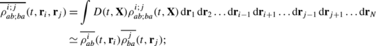
Let D(t,r ₁(t),r ₂(t),…,r _N (t))=D(t,X) be the probability density to find the system in a state with X±dX. Then the averaged probability density to find atom i in the excited state at the position r _i ±dr _i is defined as

$$ \overline{\rho_{aa}^{i}} (t,{\mathbf{r}}_{i} ) =\int D(t,{\mathbf{X}}) \rho_{aa}^{i}(t,{\mathbf{X}})\,\mathrm{d}{\mathbf{r}}_{1}\,\mathrm{d}{\mathbf{r}}_{2}\dots\mathrm{d}{\mathbf{r}}_{i-1} \,\mathrm{d}{\mathbf{r}}_{i+1}\dots\mathrm{d}{\mathbf{r}}_{N}.$$

(173)

To describe the system of atoms in different space-scale and time-scale we can develop a kinetic approximation:

• including splitting of the two-particle density matrix into a product of two one-particle density matrices

  

  (174)

  along with the Bogoljubov’s splitting approach (see, for example, [52]), that can describe vanishing the correlations between particles with time in their motion in the three-dimensional space r:

  $$\overline{f({\mathbf{r}},t)f\bigl({\mathbf{r}}',t\bigr)}\simeq\overline{f({\mathbf{X}},t)} \, \overline{f\bigl({\mathbf{X}}',t\bigr)},$$

  (175)

  where

  $$f({\mathbf{r}},t)=\int\sum^{N}_{i}\delta\bigl({\mathbf{r}}-{\mathbf{r}}_{i}(t)\bigr)\delta \bigl({\mathbf{p}}-{\mathbf{p}}_{i}(t)\bigr)\,\mathrm{d}{\mathbf{p}}$$

  (176)

  is the space distribution function, where N is total number of particles and p _i (t) is an impulse of the particle i.

In the next level of hierarchy of approximations, we can make hydrodynamic approximation:

• the local distribution function of particles in the six-dimensional velocity-coordinate space is a Maxwell-Boltzmann distribution that describes the local equilibrium state of the atoms. Then collisions between atoms will not contribute to the averaged evolution equation for the position of a physical volume element dr (Boltzmann-Enskog’ integral vanishes) (see, for example, [53]).

Therefore, we can obtain the averaged evolution equations in the following way.

As it follows from the definitions of the introduced N-particle density matrix elements,

$$\begin{array}{l}\rho^{i}_{ab}(t,{\mathbf{X}})= \bigl(\rho^{i}_{ba}(t,{\mathbf{X}}) \bigr)^{*};\\\noalign{\vspace{6pt}}\rho^{i;j}_{ab;ba}(t,{\mathbf{X}})= \bigl(\rho^{i;j}_{ba;ab}(t,{\mathbf {X}}) \bigr)^{*} \quad \hbox{and}\quad \rho^{i;j}_{ba;ba}(t,{\mathbf{X}})= \bigl(\rho^{i;j}_{ab;ab}(t,{\mathbf {X}}) \bigr)^{*};\\\noalign{\vspace{6pt}}\rho^{i;j}_{aa;ba}(t,{\mathbf{X}})= \bigl(\rho^{i;j}_{aa;ab}(t,{\mathbf {X}}) \bigr)^{*} \quad \hbox{and}\quad \rho^{i;j}_{bb;ab}(t,{\mathbf{X}})= \bigl(\rho^{i;j}_{bb;ba}(t,{\mathbf {X}}) \bigr)^{*};\end{array} $$

(177)

and, correspondingly:

$$\begin{array}{c}\rho^{i}_{ba}(t,{\mathbf{X}})-\rho^{i}_{ab}(t,{\mathbf{X}})=2 i \operatorname{Im} \bigl(\rho^{i}_{ba}(t,{\mathbf{X}}) \bigr);\\ \noalign{\vspace{6pt}}\rho^{i}_{ba}(t,{\mathbf{X}})+\rho^{i}_{ab}(t,{\mathbf{X}})=2 \operatorname{Re} \bigl(\rho^{i}_{ab}(t,{\mathbf{X}}) \bigr);\\ \noalign{\vspace{6pt}}\begin{array}{@{}l}\rho^{i;j}_{ba;ba}(t,{\mathbf{X}})+\rho^{i;j}_{ba;ab}(t,{\mathbf{X}})-\rho^{i;j}_{ab;ab}(t,{\mathbf{X}})-\rho^{i;j}_{ab;ba}(t,{\mathbf{X}})\\ \noalign{\vspace{6pt}}\quad =2 i \operatorname{Im} \bigl(\rho^{i;j}_{ba;ba}(t,{\mathbf{X}})+\rho^{i;j}_{ba;ab}(t,{\mathbf {X}}) \bigr);\end{array}\\ \noalign{\vspace{6pt}}\begin{array}{@{}l}\rho^{i;j}_{aa;ba}(t,{\mathbf{X}})+\rho^{i;j}_{aa;ab}(t,{\mathbf{X}})-\rho^{i;j}_{bb;ab}(t,{\mathbf{X}})-\rho^{i;j}_{bb;ba}(t,{\mathbf{X}})\\ \noalign{\vspace{6pt}}\quad =2 \operatorname{Re} \bigl(\rho^{i;j}_{aa;ba}(t,{\mathbf{X}})-\rho^{i;j}_{bb;ba}(t,{\mathbf {X}}) \bigr);\end{array}\\ \noalign{\vspace{6pt}}\begin{array}{@{}l}\rho^{i;j}_{ba;ba}(t,{\mathbf{X}})+\rho^{i;j}_{ba;ab}(t,{\mathbf{X}})+\rho^{i;j}_{ab;ab}(t,{\mathbf{X}})+\rho^{i;j}_{ab;ba}(t,{\mathbf{X}})\\ \noalign{\vspace{6pt}}\quad =2 \operatorname{Re} \bigl(\rho^{i;j}_{ba;ba}(t,{\mathbf{X}})+\rho^{i;j}_{ba;ab}(t,{\mathbf {X}}) \bigr).\end{array}\end{array} $$

(178)

After averaging each Eq. (7)–(10) by the distribution ${\mathcal{D}} (t,{\mathbf{X}},\dot{{\mathbf{X}}} )$ (that is probability to find the system of atoms at the phase domain $({\mathbf{X}}\pm \mathrm{d}{\mathbf{X}},\dot{{\mathbf{X}}}\pm \mathrm{d}\dot{{\mathbf{X}}} )$ in the time range t±dt) according to the rule (173), we obtain the following system of equations:

• for $\rho^{i}_{aa}$:

  

  (179)

• for $\rho^{i}_{bb}$:

  

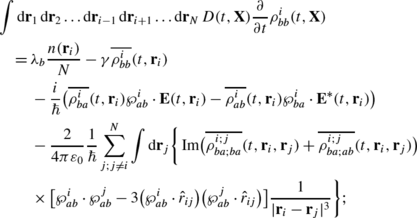  (180)

• and for $\rho^{i}_{ba}$:

  

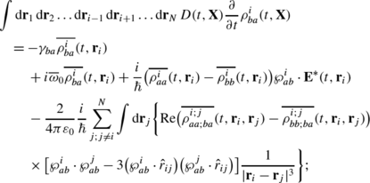  (181)

• and, finally, for the quasi-classical equation of motion:

  

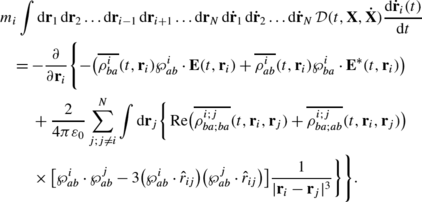  (182)

Here we used the identities:

(183)

where α∈(a,b) and β∈(a,b). And the specific normalization

(184)

where

$$D(t,{\mathbf{X}})= \int \mathrm{d}\dot{{\mathbf{r}}}_{1}\,\mathrm{d}\dot{{\mathbf{r}}}_{2}\dots \mathrm{d}\dot{{\mathbf{r}}}_{N}\, {\mathcal{D}} (t,{\mathbf{X}},\dot{{\mathbf{X}}} ).$$

(185)

Also, we note the normalization condition

$$\int _{V^{N}} \mathrm{d}{\mathbf{X}}\, D(t,{\mathbf{X}}) =\int \mathrm{d}{\mathbf{X}}\, \mathrm{d}\dot{{\mathbf{X}}}\, {\mathcal{D}} (t,{\mathbf{X}},\dot{{\mathbf{X}}} )=1,$$

(186)

where the integration over each coordinate r _i (i=1,…,N) is within the volume V, physically filled by the gas of atoms. Therefore, because of the normalization condition, or, by other words, particle number conservation in the volume V, the N-particle distributions ${\mathcal{D}}$ and D do not depend on time explicitly: the normalization condition is true for any moment time t, then

$$\frac{\partial}{\partial t} \int _{V^{N}} \mathrm{d}{\mathbf{X}}\, D(t,{\mathbf{X}}) =\frac{\partial}{\partial t} \int \mathrm{d}{\mathbf{X}}\, \mathrm{d}\dot{{\mathbf{X}}}\, {\mathcal{D}} (t,{\mathbf{X}},\dot{{\mathbf{X}}} )=0 \quad\Longleftrightarrow\quad \frac{\partial}{\partial t}D(t,{\mathbf{X}})=0.$$

(187)

Using above identities and properties we can represent the averaged partial derivative in time from the variables $\rho^{i}_{aa} (t,{\mathbf{X}} )$, $\rho^{i}_{bb} (t,{\mathbf{X}} )$, $\rho^{i}_{ba} (t,{\mathbf{X}} )$ in the following way:

(188)

here α={a,b} and α′={a,b}.

To do an approximation, we assume that two atoms become statistically uncorrelated through the quite small amount of time, such that the following expressions are true in the appropriately chosen time-scale:

$$ \begin{array}{c}\overline{\rho^{i;j}_{ba;ba}} (t,{\mathbf{r}}_{i},{\mathbf{r}}_{j})\approx \overline{\rho^{i}_{ba}} (t,{\mathbf{r}}_{i} )\overline{\rho^{j}_{ba}} (t,{\mathbf{r}}_{j} ) ;\\\noalign{\vspace{6pt}}\overline{\rho^{i;j}_{ba;ab}} (t,{\mathbf{r}}_{i},{\mathbf{r}}_{j})\approx \overline{\rho^{i}_{ba}} (t,{\mathbf{r}}_{i} )\overline{\rho^{j}_{ab}} (t,{\mathbf{r}}_{j} ) ;\\\noalign{\vspace{6pt}}\overline{\rho^{i;j}_{aa;ba}} (t,{\mathbf{r}}_{i},{\mathbf{r}}_{j})\approx \overline{\rho^{i}_{aa}} (t,{\mathbf{r}}_{i} )\overline{\rho^{j}_{ba}} (t,{\mathbf{r}}_{j} ) ;\\\noalign{\vspace{6pt}}\overline{\rho^{i;j}_{bb;ba}} (t,{\mathbf{r}}_{i},{\mathbf{r}}_{j})\approx \overline{\rho^{i}_{bb}} (t,{\mathbf{r}}_{i} )\overline{\rho^{j}_{ba}} (t,{\mathbf{r}}_{j} ).\end{array} $$

(189)

We describe here the system that consists of only identical atoms. So that, we can approximate the averaged distributions by the symmetry properties:

(190)

Then the expressions under integration in the round brackets in the evolution equations can be presented in the following way:

$$\begin{array}{c}\operatorname{Im} \bigl( \overline{\rho^{i;j}_{ba;ba}}(t,{\mathbf{r}}_{i},{\mathbf{r}}_{j} ) +\overline{\rho^{i;j}_{ba;ab}} (t,{\mathbf{r}}_{i},{\mathbf{r}}_{j} ) \bigr)\approx2 \operatorname{Im} \bigl(\rho_{ba} (t,{\mathbf{r}} ) \bigr)\operatorname{Re} \bigl(\rho_{ba} \bigl(t,{\mathbf{r}}' \bigr) \bigr);\\ \noalign{\vspace{6pt}}\operatorname{Re} \bigl( \overline{\rho^{i;j}_{aa;ba}} (t,{\mathbf{r}}_{i},{\mathbf{r}}_{j} ) -\overline{\rho^{i;j}_{bb;ba}} (t,{\mathbf{r}}_{i},{\mathbf{r}}_{j} ) \bigr)\approx \bigl( \rho_{aa} (t,{\mathbf{r}} ) - \rho_{bb} (t,{\mathbf{r}} ) \bigr)\operatorname{Re}\bigl(\rho_{ba} \bigl(t,{\mathbf {r}}' \bigr) \bigr);\\ \noalign{\vspace{6pt}}\operatorname{Re} \bigl( \overline{\rho^{i;j}_{ba;ba}} (t,{\mathbf{r}}_{i},{\mathbf{r}}_{j} ) +\overline{\rho^{i;j}_{ba;ab}} (t,{\mathbf{r}}_{i},{\mathbf{r}}_{j} ) \bigr)\approx2 \operatorname{Re} \bigl(\rho_{ba} (t,{\mathbf{r}} ) \bigr)\operatorname{Re} \bigl(\rho_{ba} \bigl(t,{\mathbf{r}}' \bigr) \bigr).\end{array} $$

(191)

Therefore, the above system of evolution equations for the densities of atomic states becomes soluble and closed on the variables that describe only “one-particle” distributions (ρ _aa (t,r), ρ _bb (t,r), ρ _ba (t,r)).

Furthermore, we suppose the local equilibrium distribution ${\mathcal{D}}$ within the volume equal to the cube of half the wave-length $\frac{ ( \pi )^{3}}{k^{3}}$. So that, the collision effects vanish after the averaging the particle i-th acceleration $\frac{\mathrm{d}\dot{{\mathbf{r}}}_{i}(t)}{\mathrm{d} t}$:

(192)

where

(193)

here $J (t,{\mathbf{X}},\dot{\mathbf{X}} )$ is the Jacobian (determinant of the Jacobian matrix $\hat{J}$) of phase coordinates transformation along the phase trajectories with time for the atoms:

$$\bigl({\mathbf{X}}(t + \mathrm{d}t),\dot{\mathbf{X}}(t + \mathrm{d} t) \bigr) = \bigl({\mathbf{X}}(t) +\delta{\mathbf{X}}(t) ,\dot{\mathbf{X}}(t) + \delta \dot{\mathbf{X}}(t) \bigr) = \hat{J} \cdot \bigl({\mathbf{X}}(t),\dot{\mathbf{X}}(t) \bigr).$$

(194)

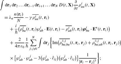
Assuming $\wp^{i}_{ab}=\wp^{i}_{ba}=\wp\hat{\wp}$, i=1,…,N, and parallel or antiparallel to the external field amplitude E, we obtain the system of the evolution equations (12)–(15) for ρ _aa (t,r) for ρ _bb (t,r), ρ _ba (t,r), and for the quasi-classical equation of motion for particles.

The equations can be easily generalized in the case of degenerated lower and upper states. In such a case it is more convenient to keep the proposed in this paper canonical form of the evolution equations with the two terms for lower and upper state populations.

1.5 A.5 Intermediate Expressions for Calculations of the Coefficients $A^{\pm}_{n}$, $B^{\pm}_{n}$, $C^{\pm}_{n}$

Substituting the expressions (37), (38), (39) into the system of Eqs. (33), (34), (35), (36), we obtain the following system of linear equations for the unknown coefficients $A^{\pm}_{n}$, $B^{\pm}_{n}$, $C^{\pm}_{n}$:

(195)

(196)

(197)

1.6 A.6 Some Properties of the Special Function “Integral Cosine” ci

The special function integral cosine has the following properties used in this paper:

$$\everymath{\displaystyle }\begin{array}{c}ci (z )\approx ci(2)+\frac{1}{2}\cos ( 2 ) (z-2 )+\biggl(-\frac{1}{4}\sin ( 2 ) - \frac{1}{8}\cos ( 2 ) \biggr) (z-2)^{2};\\\noalign{\vspace{6pt}}\mbox{where }z\in (1, 3 );\ ci (2 )\approx 0.4230;\ \sin 2\approx0.9093;\ \cos2\approx-0.4162;\end{array} $$

(198)

and

$$ci (2 \pi )\approx-0.0226; \qquad ci (z )\approx- b' +c'z, \quad \mbox{where } z\ll1, b'>0, c'>0.$$

(199)

1.7 A.7 Some Expressions

Here we propose some expressions that are intermediate on the way to obtain final result for the absorption coefficients δW and δW′ in the case of exact resonant pumping $\overline{\omega}_{0}=\omega$ with a weak back propagating “probe” field. The formulas below are obtained from the delivered in the appropriate section more general relations,

(200)

$$\tilde{C} - (\tilde{C} )^{*} = 2 \frac{1}{\gamma_{ba}}\frac{i}{\hbar}\wp\hat{\wp}\cdot {\mathbf{E}}_{0} \biggl\{ 2\tilde{A}_{0} + \frac{\hat{\wp}\cdot {\mathbf{E}}'_{0}}{\hat{\wp}\cdot{\mathbf{E}}_{0}} \bigl(\tilde{A} +\tilde{A}^{*} \bigr) \biggr\};$$

(201)

where, as one can find,

$$\tilde{A} + (\tilde{A} )^{*} = 2 \frac{\gamma_{ba} [2\gamma^{2}_{ba} +\varDelta\nu^{2} ]\tilde{a}_{r} -\varDelta\nu\gamma^{2}_{ba}\tilde{a}_{\mathrm{im}}}{(2\gamma_{ba} )^{2} + \varDelta\nu^{2}};$$

(202)

and

$$\tilde{A} - (\tilde{A} )^{*} = 2 i\frac{\gamma_{ba} [2\gamma^{2}_{ba} +\varDelta\nu^{2} ]\tilde{a}_{\mathrm{im}} +\varDelta\nu\gamma^{2}_{ba}\tilde{a}_{r}}{(2\gamma_{ba} )^{2} + \varDelta\nu^{2}}.$$

(203)

References

Hemmer, P.R., Bigelow, N.P., Katz, D.P., Shahriar, M.S., DeSalvo, L., Bonifacio, R.: Phys. Rev. Lett. 77, 1468 (1996)
Kruse, D., von Cube, C., Zimmermann, C., Courteille, Ph.W.: Phys. Rev. Lett. 91, 183601 (2003)
Bonifacio, R., McNeil, B.W.J., Piovella, N., Robb, G.R.M.: Phys. Rev. A 61, 023807 (2000)
Robb, G.R.M., Piovella, N., Ferraro, A., Bonifacio, R., Courteille, Ph.W., Zimmermann, C.: Phys. Rev. A 69, 041403 (2004)
Javaloyes, J., Perrin, M., Lippi, G.L., Politi, A.: Phys. Rev. A 70, 023405 (2004)
Mollow, B.R.: Phys. Rev. A 5, 2217 (1972)
Wu, F.Y., Ezekiel, S., Ducloy, M., Mollow, B.R.: Phys. Rev. Lett. 38, 1077 (1977)
Brown, W.J., Gardner, J.R., Gauthier, D.J., Vilaseca, R.: Phys. Rev. A 55, R1601 (1997)
Sautenkov, V.A., van Kampen, H., Eliel, E.R., Woerdman, J.P.: Phys. Rev. Lett. 77, 3327 (1996)
Li, H., Sautenkov, V.A., Rostovtsev, H.Y.V., Scully, M.O.: J. Phys. B, At. Mol. Opt. Phys. 42, 065203 (2009)
Murray, J.R., Javan, A.: J. Mol. Spectrosc. 42, 1 (1972)
Eng, R.S., Calawa, A.R., Harman, T.C., Kelley, P.L., Javan, A.: Appl. Phys. Lett. 21, 303 (1972)
Huennekens, J., Gallagher, A.: Phys. Rev. A 27, 1851 (1983)
Anderson, P.W.: Phys. Rev. 76, 647 (1949)
Dicke, R.H.: Phys. Rev. 89, 472 (1953)
Baranger, M.: Phys. Rev. 111, 481 (1958)
Griem, H.R., Baranger, M., Kolb, A.C., Oertel, G.: Phys. Rev. 125, 177 (1962)
Vdovin, Yu.A., Galitskii, V.M.: JETP 25, 894 (1967)
Zaidi, H.R.: Can. J. Phys. 55, 1229 (1977)
Kazantsev, A.P.: JETP 24, 1183 (1966)
Cooper, J.: Rev. Mod. Phys. 39, 167 (1967)
Fleischhauer, M., Yelin, S.F.: Phys. Rev. A 59, 2427 (1999)
Rautian, S.G.: JETP 91, 713–723 (2000)
Titov, E.A.: Opt. Spectrosc. 96, 869–876 (2004)
Scully, M.O., Zubairy, S.: Quantum Optics. Cambridge University Press, Cambridge (1997)
Ficek, Z., Swain, S.: In: Quantum Interference and Coherence. Theory and Experiments. Springer Series in Optical Sciences (2004)
Vorob’ev, F.A., Sokolovskii, R.I.: Zh. Prikladn. Spektrosk. 13(I), 66 (1970)
Berman, P.R.: Phys. Rev. A 59, 585 (1999)
De Salvo, L., Cannerozzi, R., Bonifacio, R., D’Angelo, E.J., Narducci, L.M.: Phys. Rev. A 52, 2342 (1995)
Lindvall, T., Tittonen, I.: Phys. Rev. A 80, 032505 (2009)
Zigdon, T., Wilson-Gordon, A.D., Friedmann, H.: Phys. Rev. A 80, 033825 (2009)
Lehmberg, R.H.: Phys. Rev. A 2, 883 (1970)
Stephen, M.J.: J. Chem. Phys. 40, 669 (1964)
Kim, M.S., de Olivera, F.A.M., Knight, P.L.: Opt. Commun. 70, 473 (1989)
Richter, Th.: Ann. Phys. (7) 40(4/5), 234 (1983)
Ikram, M., Li, F., Zubairy, M.S.: Phys. Rev. A 75, 062336 (2007)
Berman, P.R.: Appl. Phys. 6, 283–296 (1975)
Zhang, L., Yang, G.J., He, Z.H.: Phys. Lett. A 322, 166 (2004)
Maguire, L.P., van Bijnen, R., Mese, E., Scholten, R.: J. Phys. B 39, 2709 (2006)
Himsworth, M., Freegarde, T.: Phys. Rev. A 81, 023423 (2010)
Siddons, P., Adams, C.S., Ge, C., Hughes, I.G.: J. Phys. B 41, 155004 (2008)
Smith, D.A., Hughes, I.G.: Am. J. Phys. 72, 631 (2004)
Guo, J., Berman, P.R., Dubetsky, B., Grynberg, G.: Phys. Rev. A 46, 1426 (1992)
Bonifacio, R., De Salvo, L., Narducci, L.M., D’Angelo, E.J.: Phys. Rev. A 50, 1716 (1994)
Lastra, F., Wallentowitz, S., Orszag, M., Hernández, M.: J. Phys. B, At. Mol. Opt. Phys. 42, 065504 (2009)
Perrin, M., Lippi, G.L., Politi, A.: J. Mod. Opt. 49, 419 (2002)
Smirnov, M.Z.: Quantum Electron. 30, 821 (2000)
Miroshnichenko, G.P., Smirnov, M.Z.: Phys. Rev. A 64, 053801 (2001)
Grinberg, H.: J. Phys. Chem. B 112(50), 16140 (2008)
Sizhuk, A.S., Yezhov, S.M.: Derivation of the model hamiltonian in “short time scale” limit. Ukr. J. Phys. (2011, submitted)
Steck, D.A.: Sodium D line data. http://steck.us/alkalidata
Bogoljubov, N.N., Bogoljubov, N.N. Jr.: In: Introduction into Quantum Statistical Mechanics, pp. 228–245. Nauka, Moscow (1984)
Sitenko, O.G., Malnev, V.M.: In: Osnovi teorii plazmi. Naukova Dumka, Kiev (1994)
Author information
Authors and Affiliations
Corresponding author