A new nonparametric test for the race model inequality

Abstract

The race model inequality (RMI), as first introduced by Miller (Cognitive Psychology, 14, 247–279, 1982), entails an upper bound on the amount of statistical facilitation for reaction times (RTs) attainable by a race model within the redundant-signals paradigm. A violation of RMI may be considered as empirical evidence for a coactivation model rather than a race model. Here, we introduce a novel nonparametric procedure for evaluating the RMI for single participant analysis. The statistical procedure is based on a new probabilistic representation that highlights some neglected, but important distributional features of the RMI. In particular, we show how the reconstructed distribution function under maximal statistical facilitation for a race model is characterized by a specific truncated-type property. The results of two Monte Carlo simulation studies suggest that our procedure efficiently controls for type I error with reasonable power. Finally, unlike previous proposals for single participant analysis (e.g., Maris and Maris (Journal of Mathematical Psychology 47, 507–514, 2003)), our approach is also more consistent with the typical way to collect RT data in experimental works. R script functions for running the statistical analysis on single participant data are made freely available to the readers on a dedicated web server.

Introduction

A fundamental property of the human perceptual-motor system is its ability to deliver fast responses to signals presented in the environment. In the redundant signals task, the observer is required to react as quickly as possible, e.g., by pressing a response button, to the occurrence of a target stimuli. Typically, participants exhibit shorter response times (RTs) when two or more targets from different sensory modalities (visual, auditory, tactile) are presented simultaneously. The expected RT difference between single- and multiple-target conditions is called redundancy gain. In the literature, two alternative explanations have been suggested (Miller, 1982). The race model assumes that information from both targets is processed in separate sensory channels and that RT is primarily determined by the first channel (“winner of the race”) to transmit information to some more central interface in the processing hierarchy. Assuming that sensory processing time varies randomly from trial to trial, expected RT in the redundant condition is always smaller or equal to the minimum of the expected RTs in the single target conditions (Raab, 1962). Alternatively, the coactivation model assumes that redundancy gain occurs because information from each target is summed (somewhere) in the brain and that a response is triggered as soon as the combined information exceeds some threshold (Miller, 1982, 1986; Schwarz, 1994; Diederich, 1995).

The race model inequality (RMI), first suggested in Miller (1982), states that the RT distribution function for the redundant signal condition is never larger than the sum of the RT distribution functions of the two single signal conditions. Any violation of the RMI may be understood as an empirical support for a coactivation integration mechanism. In general, evaluation of the RMI has mainly been treated using statistical procedures for group data (e.g., Miller, 1982; Ulrich et al.,, 2007; Gondan, 2010), while statistical approaches for testing the RMI in single participant’s data is less common (e.g., Miller, 1986; Maris & Maris, 2003; Vorberg, 2008). A first proposal for analyzing data in single participants appeared in a seminal work by Miller (1986) in which the violation of the RMI was evaluated using a bootstrapping procedure (Efron, 1979). More recently, a nonparametric test based on a modified version of the ordinary Kolmogorov–Smirnov (KS) statistic was introduced by Maris and Maris (2003). It was based on a probabilistic sampling procedure associated with a mixture distribution with equal weights for the two single target conditions. In practice, this procedure required that in each single signal trial a fair coin was tossed to determine in which channel the stimulus was presented next. This mixture distribution paradigm, however, had several practical limitations and was rarely met in most experimental work.

In this paper, we take advantage of the original idea introduced by Maris and Maris (2003) but reformulate it to propose a new nonparametric statistical procedure for evaluating the race model inequality for single-participant analysis. We will introduce a novel probabilistic context that highlights some neglected, but relevant distributional properties of the RMI. In particular, the proposed procedure is more consistent with the typical way to collect RT data in experimental works.

The manuscript is organized as follows. The next section specifies the RMI at both the population and sample level. Some relevant properties of the distribution functions associated with the RMI are discussed and a new statistical procedure based on a truncated version of the KS statistic is presented. In the third section, two simulation studies are reported to evaluate performance of the new statistical procedure. Finally, the fourth section presents discussion and conclusions.

Evaluating the race model inequality

In the redundant condition, let (S₁, S₂) be a pair of (jointly distributed) continuous random variables with S₁ the processing time for the first channel and S₂ for the second channel. Under the race model, define

$$ Z = \min(S_{1},S_{2}) $$

(1)

as random variable representing observable response time in the redundant condition, whereas S₁ and S₂ are considered unobservable variables (only their minimum is). According to the assumption of context invariance (Miller, 1982; Colonius, 1990; Luce, 1986), the marginal distributions of S₁ and S₂ are equal to the distributions of the RT random variables X and Y observed in the single target conditions, respectively.¹

Under context invariance, the distribution F_Z of Z equals:

$$ F_{Z}(t) = F_{X}(t) + F_{Y}(t) - P(S_{1} \leq t,S_{2} \leq t) $$

(2)

where F_X and F_Y are the distribution functions of X and Y, respectively.² The latter equation implies the following inequality:

$$ F_{Z}(t) \leq \min\{1,F_{X}(t) + F_{Y}(t)\}, \quad \text{for all } t $$

(3)

It provides an upper bound for RT in the redundant condition under the race model and is called race model inequality (Miller, 1982). Writing

$$ K(t) = \min\{1,F_{X}(t) + F_{Y}(t)\}, \quad \text{for all } t, $$

(4)

then F_Z = K corresponds to a race model under maximal attainable statistical facilitation. More precisely, if S₁ and S₂ show maximum negative stochastic dependence with fixed marginals F_X and F_Y (Miller, 1982; Colonius, 1990, 2016), then a coupling exists (i.e., a bivariate distribution with maximal negative correlation) such that

$$\begin{array}{@{}rcl@{}} P(S_{1} \leq t_{1},S_{2} \leq t_{2}) & = & C_{S_{1}S_{2}}(t_{1},t_{2})\\ & = & \min\{F_{X}(t_{1}),F_{Y}(t_{2})\}, \qquad \forall t_{1}, \forall t_{2} \end{array} $$

with the mapping $C_{S_{1}S_{2}}$ being a copula and where its diagonal section (t₁ = t₂) yields

$$F_{Z}(t) = K(t), \quad \text{for all } t. $$

Clearly, if F_Z(t) > K(t) for some t, then the redundant signals effect is no longer compatible with predictions from the race model under context invariance. Distribution function K(t) will be referred to as reconstructed distribution function below.

On the basis of the statistical facilitation principle and the context invariance assumption, we can formulate the following null hypothesis for testing the RMI:

$$ H_{0} : F_{Z}(t) \leq K(t), \quad \text{for all } t. $$

(5)

Since under the null hypothesis the distribution F_Z is most to the left if F_Z = K, we set the corresponding point null hypothesis as follows

$$ H_{0}^{\ast} : F_{Z}(t) = K(t), \quad \text{for all } t. $$

(6)

Population-level representation

In what follows, we will illustrate some relevant properties regarding the reconstructed distribution function K. Note that definitions, propositions, and corollaries are enumerated sequentially as they appear. We first introduce the so-called average distribution for the single-channel conditions:

$$ M(t) = \frac{1}{2} (F_{X}(t) + F_{Y}(t)). $$

(7)

The average distribution M is a mixture distribution where the two original distribution functions F_X and F_Y have equal weights. In our context, it is important to note that this mixture distribution constituted the main probabilistic token described by Maris and Maris (2003) in their original proposal. Here we will show how to modify this representation to adapt it to our new framework.

Definition 1

Let p ∈ (0, 1) and ξ_p = M^− 1(p) = inf{t : M(t) ≥ p} the p-quantile for the average distribution M. The p-truncated average distribution is represented as follows:

$$ M_{p}(t)= \left\{ \begin{array}{ll} M(t)/M(\xi_{p}), & 0 < t \leq \xi_{p} \\ 1, & t > \xi_{p} \\ 0, & t = 0 \end{array} \right. $$

(8)

The p-truncated average distribution represents a measure of the fraction of the average distribution M up to the p-th quantile. The following proposition details the close relationship between an important instance of the truncated average distribution M_p and the reconstructed distribution K.

Proposition 2

The reconstructed distribution function K for the redundant condition is equivalent to the 0.5-truncated averagedistribution:

$$ K(t) = M_{0.5}(t), \quad \text{for all \textit{t}}. $$

(9)

Proof

First, for all t ≤ 0 both distribution functions always take value 0 as F_X and F_Y have nonnegative arguments. Next, suppose that 0 < t ≤ ξ_0.5, then

$$\begin{array}{@{}rcl@{}} M_{0.5}(t) & = & M(t)/M(\xi_{0.5})\\ & = & M(t)/0.5\\ & = & 2M(t)\\ & = & K(t), \end{array} $$

as for all positive t that never exceed the 0.5-quantile of M, the rescaled distribution function 2M(t) cannot exceed 1. Finally, for all values of t > ξ_0.5 we have that M(t) > 0.5 and consequently 2M(t) > 1 and so K(t) = 1. The same goes with M_0.5(t) as by construction this distribution function is truncated at ξ_0.5. □

Corollary 3

Under the maximal statistical facilitation assumption of a race model we have that:

$$F_{Z}=M_{0.5}.$$

Proof

Trivial. It immediately follows from Proposition 2 and the definition of the point null hypothesis (6). □

In sum, the most relevant result of this section regards the characterization of the reconstructed RST distribution function K as a truncated-type distribution with truncation point localized at the population quantile ξ_0.5 of M. Moreover, under the point null hypothesis (6) also the RT distribution for the original redundant condition F_Z must be characterized by exactly the same property. To our knowledge, this is the first time that this peculiar property about K has been explicitly characterized in the RMI literature. Later on in this paper (e.g., in the test procedure section), it will become clear how the truncation property of K directly plays a key role in the definition of the statistical test for the evaluation of the RMI in the redundant signals paradigm.

Sample level representation

In this section, we will introduce our main idea about the sampling procedure for the random variables involved in the RMI and the estimation of the corresponding distributions. Here, we will also highlight the more relevant differences (at the sample level) between our approach and the original proposal by Maris and Maris (2003).

Let us assume that the redundant signal (RST) condition is associated with m distinct trials whereas the two single signal (SST) conditions are associated with n₁ and n₂ trials, respectively. Moreover, let $\mathscr{Z}=\{Z_{1},Z_{2},\ldots ,Z_{m}\}$, $\mathscr{X}=\{X_{1},X_{2},\ldots ,X_{n_{1}}\}$, and $\mathscr{Y}=\{Y_{1},Y_{2},\ldots ,Y_{n_{2}}\}$ be the corresponding sets of random variables. In our context, we assume that each of the three sets is composed of independent identically distributed (i.i.d.) random variables with cumulative distribution functions (cdf) F_Z, F_X and F_Y, respectively. Taken together, the two SST conditions yield a combined set $\mathscr{W}=\mathscr{X} \cup \mathscr{Y}=\{X_{1},\ldots ,X_{n_{1}},Y_{1},\ldots ,Y_{n_{2}}\}$ of n₁ + n₂ elements. In our representation, we also assume that all pairs $(X,Y) \in \mathscr{X} \times \mathscr{Y}$ are independent. The latter independent coupling condition (Colonius, 2016) may easily be motivated by considering that the observations in the two SST conditions are usually recorded in separate experimental trials.³ In sum, the combined set $\mathscr{W}$ is understood as a collection of n₁ + n₂ independent and non-identically distributed random variables (e.g., Van Zuijlen, 1978).

Definition 4

Given the combined set $\mathscr{W}$, the average cumulative distribution function of $\mathscr{W}$ is represented as follows:

$$ A(t) = \frac{1}{n_{1} + n_{2}} (n_{1}F_{X}(t)+n_{2}F_{Y}(t)). $$

(10)

Unlike the average distribution M, the structure of A clearly depends on the relative frequencies of the random variables in $\mathscr{W}$ for the two classes of distributions F_X and F_Y. Here we will highlight a relevant property of A when equal sample sizes are considered.

Proposition 5

For all sample sizes n, ifn₁ = n₂ = n,then the average distribution A reduces to the population average distribution M.

Proof

Trivially, for any n = 1,2,…,

$$\begin{array}{@{}rcl@{}} A(t) & = & \frac{1}{2n} (nF_{X}(t)+nF_{Y}(t))\\ & = & \frac{1}{2} (F_{X}(t)+F_{Y}(t))\\ & = & M(t), \end{array} $$

for all t. □

Note that, unlike the average mixture distribution, here A literally represents the average of distributions associated with a fixed number 2n of independent and (non)identically distributed random variables. The latter makes the sampling procedures for the two representations quite different. In particular, for the average mixture distribution M, the sampling always requires that each time an SST trial is administered in an experiment, a fair coin is tossed to determine to which channel the next stimulus is presented (e.g., Maris & Maris, 2003). By contrast, for the averaged distribution A (with equal sample sizes), we have a fixed number n of trials for each of the two SST conditions. Even if the two sampling procedures asymptotically converge to the same empirical distribution (i.e., when n → + ∞), they may substantially deviate for small to medium sample sizes. In this work, we will take advantage of the equal sample size assumption to illustrate some useful estimation procedures for the reconstructed distribution function K. In particular, in the estimation of K, we will replace the estimator of M_0.5(t) in Eq. 9 with the corresponding estimator of A_0.5(t) based on the observed experimental data for the combined set $\mathscr{W}$.

Now, let z, x, and y be random samples associated with $\mathscr{Z}$, $\mathscr{X}$, and $\mathscr{Y}$, respectively. Hereafter, we assume that x and y have equal sample size n while z has size m with no ties in the full data set.⁴ Let $\widehat {F}_{Z,m}$, $\widehat {F}_{X,n}$, and $\widehat {F}_{Y,n}$ be the corresponding empirical distribution functions (ecdfs) associated with the three samples. It is well known that ecdfs are consistent and unbiased estimators of the associated distribution functions under representative sampling (e.g., Pratt & Gibbons, 1981). Moreover, because all transformations described in Eqs. 4, 7 and 9 are continuous mappings, it follows that $\widehat {K}$, $\widehat {A}$, and $\widehat {A}_{0.5}$ are also consistent estimators of K, A, and A_0.5, respectively (Serfling, 1980). In particular, the reconstructed distribution K can be estimated using one of the following three equivalent procedures:

$$\begin{array}{@{}rcl@{}} \widehat{K}(t) & = & \min\{1,\widehat{F}_{X,n}(t) + \widehat{F}_{Y,n}(t)\} \end{array} $$

(11)

$$\begin{array}{@{}rcl@{}} & = & \min\{1,2\widehat{A}(t)\} \end{array} $$

(12)

$$\begin{array}{@{}rcl@{}} & = & \widehat{A}_{0.5}(t) \end{array} $$

(13)

where $\widehat {A}^{-1}(0.5)=\widehat {\xi }_{0.5}=\inf \{t: \widehat {A}(t) \geq 0.5\}$ is the empirical 0.5-quantile computed on $\widehat {A}$. However, under the equal sample size assumption, the estimator for K can also be directly computed from the combined sample vector w = (x,y). In particular, the ecdf of w represents a direct estimator of the averaged distribution A. Similarly, the empirical 0.5-quantile $\widehat {\xi }_{0.5}$ for $\widehat {A}$ is also equivalent to the n-th ordered value w_(n) in w. Therefore, a direct estimation of K can be obtained by computing the ecdf on the subsample of w composed of its first n-ordered observations: w₍₁₎, w₍₂₎,…,w_(n). Table 1 reports a hypothetical data set which may serve as a guiding example to illustrate the different estimation procedures considered here. Several properties of the (empirical) averaged distribution functions and their relations with order statistics have been extensively investigated in the statistical literature (e.g., Van Zuijlen, 1976, 1978).

Table 1 Hypothetical data based on a uniform model for F_X and F_Y

Note that, at the sample level, the main difference between our proposal and the mixture representation by Maris and Maris (2003) pertains to the way the reconstructed distribution K is estimated. In particular, in the mixture representation, $\widehat {K}$ is estimated as follows

$$\widehat{K}(t) = \min\{1,2\widehat{M}(t)\} $$

with $\widehat {M}$ being the ecdf of the mixture sample drawn from the population mixture distribution M (see Eq. 7), which makes the two proposals clearly different at the sample level as detailed earlier in the manuscript.

We conclude this section by highlighting some important relationships regarding the maximal statistical facilitation property for a race model, the combined set $\mathscr{W}$, and the antithetic variates method for continuous random variables. We recall that the method of antithetic variates (e.g., Thompson, 2000; Colonius & Diederich, 2006) can be used to generate a pair of maximally negative dependent random variables from the two SST conditions in line with the maximal statistical facilitation assumption for the RMI (Miller, 1982; Colonius, 1990).

Definition 6

Let X₍₁₎, X₍₂₎,…,X_(n) and Y₍₁₎, Y₍₂₎,…, Y_(n) denote the order statistics for the sets $\mathscr{X}$ and $\mathscr{Y}$, respectively. The antithetic variates transformations are defined as follows:

$$\begin{array}{@{}rcl@{}} R_{i} & = & \min\{X_{(i)},Y_{(n-i + 1)}\}, \end{array} $$

(14)

$$\begin{array}{@{}rcl@{}} T_{i} & = & \max\{X_{(i)},Y_{(n-i + 1)}\}, \qquad i = 1,\ldots,n. \end{array} $$

(15)

Note that the distribution of the antithetic variates R_i (i = 1,…,n) corresponds to the reconstructed distribution for the redundant condition under maximal statistical facilitation. That is to say: F_R = K as defined in Eq. 4.

Proposition 7

LetW₍₁₎, W₍₂₎,…,W_(2n),(n even) denote the orderstatistics for the set$\mathscr{W}$,then

$$W_{(i)} = R_{(i)} \quad \text{and} \quad W_{(n+i)} = T_{(i)}, \qquad i = 1,\ldots,n. $$

Proof

The problem stated here is a particular instance of merging networks, which are networks that can merge two sorted input sequences into one sorted output sequence (called Merger[n] in Cormen et al.,, 2001). Specifically, R_(i) and T_(i) (i = 1,…,n) are the two sorted input sequences and W_(i) with (i = 1,…,2n) corresponds to the sorted output sequence. For details, see Cormen et al. (2001, pp. 716–718). □

Notice, however, that the close relationship between the combined set $\mathscr{W}$ and the antithetic variates method can be further generalized to all positive integer n (not necessarily even) as highlighted in the following remark.

Remark 8

The identity F_R = A_0.5 follows by Proposition 2 and 5. Moreover, at the sample level, $\widehat {A}^{-1}(0.5)=\widehat {\xi }_{0.5}=w_{(n)}$ and consequently r_(i) = w_(i) for all i = 1,2,…,n. A similar construction can be verified for the remaining half sample w_{(n + i)} (i = 1,2,…,n) of w with respect to the corresponding antithetic variate quantities t_(i). Note that this line of reasoning simply requires that n be a natural number (either even or odd).

To summarize, the most relevant result of this section regards the characterization of the reconstructed RST distribution function K as a truncated distribution under the point null hypothesis (6). Moreover, Proposition 7 shows that computing an antithetic variates transformation simply coincides with directly selecting the first n order statistics from the combined set $\mathscr{W}$. Overall, this means that in the estimation of the cdf K the adoption of (i) the procedures described in Eqs. 11, 12 and 13, (ii) the ecdf computed on the first n ranked elements of the combined data set w, and finally (iii) the ecdf computed on the output of the antithetic variates approach (14), constitute all legitimate and equivalent estimators for K. In the next section, we will use these specific features of the reconstructed cdf K to suggest a statistical test procedure that accounts for its truncation property in comparing the empirical distribution functions in the RST and SST conditions.

The test procedure

The null hypothesis (5) entails that, under the RMI, the cdf F_Z of the RST condition never dominates the reconstructed cdf K. As a consequence, under the null hypothesis we generally expect that $\widehat {F}_{Z,m}(t)$ should have smaller or equal values than $\widehat {K}(t)$ for all values t ≥ 0. In line with Maris and Maris (2003), we opted for a signed Kolmogorov-Smirnov (KS) test approach to evaluate this condition. In general, the KS test can be used to compute a distance between the two ecdfs as follows:

$$\begin{array}{@{}rcl@{}} d^{+} & = & D^{+}(\mathbf{z},\mathbf{w}) \\ & = & \max\limits_{t}[\widehat{F}_{Z,m}(t)-\widehat{K}(t)] \\ & = & \max\limits_{t}[\widehat{F}_{Z,m}(t)- \min\{1,2\widehat{A}(t)\}] \\ & = & \max\limits_{t}[\widehat{F}_{Z,m}(t)- \widehat{A}_{0.5}(t)] \end{array} $$

(16)

However, because under the maximal statistical facilitation assumption the reconstructed distribution K is always characterized by a truncated feature, we need to modify the KS test to account for this specific distributional feature (Tsao, 1954; Conover, 1967; Barr & Davidson, 1972; Koziol & Byar, 1975; Grover, 1977; Dufour & Maag, 1978; Michael & Schucany, 1979). In particular, a simple adaptation of the KS test which accounts for truncated distributions is as follows:

$$ d_{tru}^{+} = \max_{t \leq t^{\ast}}[\widehat{F}_{Z,m}(t)- \widehat{K}(t)] $$

(17)

where t^∗ = min{w_(n), z_(m)} is the common threshold value for the two ecdfs and z_(m) is the maximum value for z. Moreover, because under the point null hypothesis (6) the ecdf $\widehat {F}_{Z,m}$ tends to be largest everywhere, we also expect that under this condition also $d_{tru}^{+}$ should reflect largest deviation values. Note that, Eq. 17 highlights another important difference between our approach and the mixture representation by Maris and Maris (2003). In particular, in their proposal the statistical test did not require any kind of truncation correction as evident from their Kolmogorov-Smirnov distance equation:

$$d_{mix}^{+} = \max_{t}[\widehat{F}_{Z,m}(t) - \min\{1,2\widehat{M}(t)\}]. $$

Moreover, in the computation of the distance measure the ecdf of the mixture distribution M was adopted in place of the ecdf of the average distribution A.

Since the ordinary KS statistic, as well as its truncated (resp. mixture) version are invariant under the probability integral transformation of the underlying data, there is no loss of generality in limiting the discussion of these tests to the case of the uniform transformations (Angus, 1994; Barr & Davidson, 1972). In particular, in the truncated version of the KS statistic, the sample distribution functions can be viewed as random walks from the origin (0,0) to the truncation point t^∗ once it has been rescaled under the uniform distribution. Finally, we can easily approximate the probability distribution of $D_{tru}^{+}$ under the point null hypothesis by adopting the following simple simulation procedure.

Generating the null distribution

The main idea consists in generating transformed sample arrays for the SST and RST conditions under the point null hypothesis (6) on the basis of the simple algorithm described in Table 2. The data-generation algorithm is then used to approximate the probability distribution of $D_{tru}^{+}$ under the point null hypothesis to any degree of precision. In particular, to generate the point null distribution for the truncated version of the KS statistic, we revolve in setting the following three steps:

• 1. Simulate a large number N (e.g., N = 10,000) of transformed uniform samples, u^∗ and v^∗, for the SST and RST conditions as detailed in Table 2.

• 2. For each pair of transformed uniform samples (u^∗, v^∗) compute $\widehat {K}$ on u^∗ and $\widehat {F}_{Z,m}$ on v^∗. Finally, compute the simulated truncated KS test $c_{tru}^{+}$ according to (17) with t^∗ = min{u_(n), v_(m)}.

• 3. Derive an approximated p value by using the proportion of generated N values, $c_{tru}^{+}$, that exceeds the empirical sample value $d_{tru}^{+}$.

Table 2 Data generation algorithm. U(0, 1) denotes the uniform distribution

Note that under the probability integral transformation, the derivation of the distribution function $F_{T^{\ast }}$ for the common threshold T^∗ = min{U_(n), V_(m)} is straightforward (see also Table 2). In the following proposition, we will derive the analytic representation for the distribution of T^∗.

Proposition 9

Under the point null hypothesis, the distribution function$F_{T^{\ast }}$forthe common threshold variableT^∗,computed on arrays of independent and uniformly distributed r.v.s (U₁,…,U_2n) and (V₁,…,V_2m),takes the following form:

$$\begin{array}{@{}rcl@{}} F_{T^{\ast}}(x) &=& I_{x}(n,n + 1) + I_{x}(m,m + 1)\\ &&- I_{x}(n,n + 1)I_{x}(m,m + 1), \end{array} $$

(18)

with 0 < x < 1 andwhereI_x(a,a + 1) isthe regularized beta function

$$ I_{x}(a,a + 1) = \frac{1}{B(a,a + 1)}{{\int}_{0}^{x}} c^{(a-1)}(1-c)^{a} dc, $$

(19)

withBbeing the ordinary beta function anda > 0.

Proof

From the basic theory on order statistics (e.g., Arnold et al.,, 2008), we have that the distribution function for T^∗ is given by

$$\begin{array}{@{}rcl@{}} F_{T^{\ast}}(x) & = & P(T^{\ast} \leq x)\\ & = & 1 - P(T^{\ast} > x)\\ & = & 1 - [1 - F_{U_{(n)}}(x)][1 - F_{V_{(m)}}(x)] \end{array} $$

with $F_{U_{(n)}}$ and $F_{V_{(m)}}$ being the distribution functions for the order statistics U_(n) and V_(m), respectively. Moreover, for independent and uniformly distributed random variables, it is known that

$$\begin{array}{@{}rcl@{}} F_{U_{(n)}}(x) & = & I_{x}(n,n + 1) \end{array} $$

(20)

$$\begin{array}{@{}rcl@{}} F_{V_{(m)}}(x) & = & I_{x}(m,m + 1) \end{array} $$

(21)

and therefore

$$\begin{array}{@{}rcl@{}} F_{T^{\ast}}(x) & = & 1 - [1 - I_{x}(n,n + 1)][1 - I_{x}(m,m + 1)]\\ & = & I_{x}(n,n + 1) + I_{x}(m,m + 1) - I_{x}(n,n + 1)\\ &&I_{x}(m,m + 1), \end{array} $$

by simple algebra. □

Note that the expected values and variances for the order statistics U_(n) and V_(m) are, respectively,

$$\begin{array}{@{}rcl@{}} E(U_{(n)}) &=& \frac{n}{2n + 1} \qquad Var(U_{(n)}) = \frac{n^{2}+n}{(2n + 1)^{2}(2n + 2)},\\ E(V_{(m)})\! &=&\! \frac{m}{2m + 1} \!\qquad \!Var(V_{(m)}) = \frac{m^{2}+m}{(2m + 1)^{2}(2m + 2)}, \end{array} $$

which make U_(n) and V_(m) consistent but biased estimators of the uniform population quantile ξ_0.5(= 0.5). The latter entails that also T^∗ is a consistent but biased estimator of ξ_0.5, where in particular it underestimates the population median 0.5 of the uniform distribution. However, it is worthwhile noticing that this biased feature is typical for any random sample with an even number of observations and it does not affect the overall functioning of the truncated statistic. More information about the basic properties of the truncated KS statistic can be find in the nonparametric statistics literature (e.g., Tsao, 1954; Conover, 1967; Barr & Davidson, 1972; Koziol & Byar, 1975; Grover, 1977; Dufour & Maag, 1978; Michael & Schucany, 1979).

R script functions

The testing procedure based on the truncated Kolmogorov–Smirnov test is implemented using a set of R script functions, which only require the base R package (R Core Team, 2018) to be installed. The R script functions work with raw observed reaction times for the three samples of observations, x, y, and z, and can be collected with any recording software capable to export data in .csv format. The R scripts are freely available at [http://www.polorovereto.unitn.it/~luigi.lombardi/TestingRMI.html] together with an associated documentation illustrating the application of the R scripts via simple examples of data analysis.

Simulation studies

In this section, we will test the behavior of the proposed algorithm by means of two simulation studies and compare its results with the original nonparametric test introduced by Maris and Maris (2003). The first simulation will investigate the type I error rate as a function of factors such as sample size and distributional features. The second simulation will be focused on some statistical power aspects of the truncated Kolmogorov–Smirnov test.

Type I error rate

To evaluate the performance of the new statistical procedure, we ran a Monte Carlo (MC) simulation study to investigate the type I error rate. The analysis was conducted within the point null hypothesis framework: H₀ : F_Z(t) = K(t), ∀t ≥ 0. In this context, both $\widehat {F}_{Z,m}$ and $\widehat {K}$ were constructed in order to correspond to the maximal statistical facilitation attainable for a race model. Both single target conditions and redundant target condition were modeled according to a Weibull distribution (Van Zandt, 2000; Palmer et al., 2011). We recall that the Weibull distribution is characterized by two parameters: scale (λ) and shape (k). In this and in the following simulation study, only non-scaled observations were considered (as the Maris and Maris’s KS test as well as the truncated KS test are known to be scale invariant). The simulation was performed by systematically varying two factors in a complete 4 × 5 two-factorial design (see also Rach et al.,, 2010). In particular, the factors were:

• (i) the distance rate (δ) at four levels: 0, 0.1, 0.2, 0.3. Factor δ regulates the relation between the distributions of the two channels (X and Y ) for the two single target conditions. This relation is modeled by increasing an initial parameters array Θ₀ = (λ₀, k₀) according to Θ_i = Θ₀ + δ_iΘ₀, i = 1,2,3,4. The single target conditions are modeled by keeping fixed Θ₀ for X, and by letting Θ_i to vary along the levels of the factor, for Y. Initial parameter values were fixed at λ₀ = 1.5 and k₀ = 100 (Fig. 1);

  Fig. 1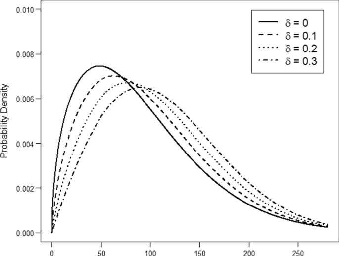

  

  Distributions of the channels for single signal conditions when varying the levels of factor δ. Note that, when δ = 0, the distribution of X and that of Y perfectly overlap

• (ii) the sample size (s) at five levels: 20, 50, 100, 250, 500.

For each of the four distributional patterns (conveyed by the levels of δ), 10,000 simulations were performed for each level of s (here we assume that m = n = s). On the basis of these simulations, we computed the proportion of rejections of the null hypothesis for all the combinations of the factor levels. Table 3 reports the results of this first simulation study, that is, the type I error rate as a function of distance rate and sample size for the two statistical procedures. To summarize, under the framework of the point null hypothesis, no particular effects of the factors on the type I error rate were observed. Overall, for the truncated KS test, the error rate approximately settled on the expected value (5%), whereas the Maris and Maris KS test showed sub-optimal performances. In particular, for the mixture KS test, the H0 rejection rates were above 10% in many simulated conditions.

Table 3 Type I error rate (as percentage of rejections) for the truncated Kolmogorov–Smirnov test and the mixture Kolmogorov–Smirnov test (in parenthesis)

Power analysis

In this section, we present a more realistic scenario in which the (non-scaled) RT distribution F_Z for the redundant target condition is modeled in a more natural and plausible way. In this second simulation study, we considered several redundant target conditions in which the distributional patterns were not constructed to reflect a maximal statistical facilitation (and therefore a truncated distribution for F_Z). Also, in this second simulation, the observed responses were modeled according to a Weibull distribution and assumed equal sample size (n = m = s) for F_Z and K (Rach et al., 2010). In the simulation design, we varied three factors in a complete 4 × 5 × 10 factorial design. The factors were:

• (i) the distance rate (δ) at four levels: 0, 0.1, 0.2, 0.3;

• (ii) the sample size (s) at five levels: 20, 50, 100, 250, 500;

• (iii) the shape scaling factor (η) at ten levels: 0.0159, 0.0169, 0.0179, 0.0189, 0.0199, 0.0209, 0.0219, 0.0229, 0.0239, 0.0249. Factor η regulates the shape parameter (k) of the redundant target condition distributions according to $k_{r}=\frac {1}{\eta _{r}}$ for r = 1,2,...,10.

The aim of this new simulation study was to analyze the proportion of rejection of H₀ under different conditions, that is, different distributional patterns of single and redundant target conditions in which specific violations may occur. In particular, four overall patterns of RMI violation magnitude blocks were generated, one for each level of δ. For each δ-block, the reconstructed RST distribution K was generated according to the maximal statistical facilitation hypothesis for a race model. By contrast, F_Z was generated as the cdf of Z with $Z \sim Weibull\left (\lambda _{i},k_{r}=\frac {1}{\eta _{r}}\right )$ where λ_i = λ₀ + δ_iλ₀ and λ₀ = 1.5. These redundant target condition distributions are meant to elicit a violation of the race model inequality to varying magnitudes. The higher the value of η_r, the greater the magnitude of the violation (Fig. 2).

Fig. 2

Distributional pattern block for the power analysis (δ = 0.2). In the block, we generated ten different distributions for F_Z, one for each level of η. The truncated distribution (thick solid line) represents K. Dotted vertical lines represent the medians of the redundant target distributions F_Z. The thick line represents the median of K

Four power analyses were conducted, one for each of the four blocks of violation magnitude patterns. A total of 10,000 simulations were performed for each combination of levels of δ, s, and η.⁵ The dependent variable was the proportion of rejection of the null hypothesis (H₀ : F_Z ≤ K) for the two statistical tests.

For the sake of space, we limit here the presentation of our results to the δ = 0.2 condition only.⁶ Table 4 reports the results concerning the violation magnitude patterns as a function of the sample size and median gainMG (resp., maximum theoretical distanceMTD) for δ = 0.2. The median gain can be computed as the difference between the median of K and the median of F_Z. As expected, negative values for the median gain were more associated with larger approximated p value (Fig. 3). By contrast, positive median gains are associated with a violation of the race model inequality (Fig. 3).

Table 4 Power analysis (as percentage of rejections) for the truncated Kolmogorov–Smirnov test (first row), and the mixture Kolmogorov–Smirnov test (second row). MG median gain, MTD maximal theoretical distance

Fig. 3

Power analysis as a function of sample size and distance information for block δ = 0.2. The first row of the horizontal axis shows the median gain, whereas the second row shows the maximum theoretical distance. Black lines denote the power curves for the truncated KS test. Blue lines indicate the power curves for the mixture KS test

However, the median gain only provides a horizontal measure of distance and does not provide an effective measure of theoretical violation which is, instead, yielded by the maximum theoretical distance (MTD) between the two distributions. Both median gain and maximum theoretical distance were computed in order to compare the rejection rates according to readable indices of violation. The results showed that, indeed, by increasing the positive median gain (resp. maximum theoretical violation), the proportion of rejections for H₀ also increased in both statistical tests (truncated KS test and mixture KS test). Finally, as expected, rejection rates were also clearly affected by the sample size factor with larger samples being associated with larger probabilities of rejecting the null model when H₀ was false (Fig. 3). However, one clear difference emerged between the two statistical procedures. The truncated KS test was more conservative for small samples but resulted more powerful with medium or large samples as compared to the mixture KS test. This is not a surprise, as in the previous simulation study, the mixture KS test failed in controlling the type I error rate. The same results were observed for the remaining conditions of the simulation study, which are reported in the supplementary material.

Taken together, the two simulation studies show that the truncated KS test efficiently controls for type I error and it is also characterized by a reasonable power. By contrast, the statistical test based on the mixture representation (Maris & Maris, 2003) appears somehow flawed. In particular, it does not seem to adequately control for the rejection rate under H0. It also shows (at some levels) less power as compared to our proposal, specifically in the asymptotic conditions where large sample sizes are considered. At the same time, the mixture KS test seems to be too sensitive in small samples scenarios which, in turn, should naturally be considered less reliable. In the supplementary material, we finally reported the results of an additional simulation study based on the well-known diffusion superposition model for reaction times (Schwarz, 1994), which generally confirmed the results of the power simulation study described in this section.

Discussion and conclusions

In this paper, we first studied the truncated property of the reconstructed distribution K for the redundant condition and, subsequently, proposed a new nonparametric procedure (based on a modified version of the KS test) to evaluate violation of the race model inequality in the single-participant analysis context. To our knowledge, this is the first time that this property has been explicitly studied in the RMI framework. In particular, we showed that under an equal sample size assumption for the two SST conditions, estimation of the reconstructed distribution K can be obtained using a variety of perfectly equivalent procedures (e.g., antithetic variates method, ecdfs transformations, truncated sample derivation), which all yield the same consistent estimator for K. In addition, by using the averaged representation for the combined set $\mathscr{W}$, we were also able to propose a new, simple simulation algorithm (based on the probability integral transformation) to approximate, to any level of desired precision, the distribution of the test statistic under the null hypothesis. The corresponding sampling procedure nicely overcame some inherent limitations of applying the mixture representation as originally proposed by Maris and Maris (2003). Indeed, in experimental contexts, participants are typically presented a fixed number of trials from each of the two SST conditions, instead of a random assignment as required by the mixture sampling procedure.

Regarding the performance of the new statistical test, the results of two Monte Carlo simulation studies suggested that our procedure efficiently controlled for type I error when a point null hypothesis F_Z = K was true. By contrast, the mixture KS test failed in controlling the type I error, as it showed a larger proportion of H₀ rejections (> 0.05). As for power analysis, the truncated version of the KS test was in general able to reject the null hypothesis when a violation of the race model inequality occurred at the population level. As expected, the power of the statistic was positively related with sample size. Overall, the results of these preliminary simulation studies seem to support the validity of the new statistical proposal.

To conclude this section, we now discuss some potential concerns associated with our statistical framework. First, we consider the consequences of relaxing the equal sample size assumption for the two SST conditions in testing the RMI. In some circumstances, one may face the problem of unbalanced data for the two SST conditions due, for example, to missing observations caused by omitted responses, errors, or outliers. Alternatively, in some experiments we may observe unbalanced data because of specific experimental designs or requirements. In all these situations, a tempting solution could be estimating K according to:

$$ \widehat{K}(t) = \min\{1,\widehat{F}_{X,n_{1}}(t) + \widehat{F}_{Y,n_{2}}(t)\}, \qquad t \geq 0 $$

(22)

with n₁≠n₂. However, although the two ecdfs $\widehat {F}_{X,n_{1}}$ and $\widehat {F}_{Y,n_{2}}$ are consistent and unbiased estimators of F_X and F_Y, the reconstructed distribution $\widehat {K}$, as defined in (22), generally is no more an ecdf. In particular, the resulting $\widehat {K}(t)$ would not necessarily be a step function with equal fixed jumps which, in turn, represents a mandatory property for any well-formed ecdf.⁷ Note that this problem disappears when sample sizes are equal. For n₁ = n₂ = n, the reconstructed $\widehat {K}$ is always an ecdf (i.e., a step function that jumps up by 1/n at each of the n data points), and hence is also a consistent estimator of K. Similarly, it would not be clear how to estimate K using directly the combined sample w or the antithetic variates method. In general, for unbalanced data, a possible way out could be the adoption of a resampling procedure with which we repeatedly sample a subset of n^∘ = min{n₁, n₂} observations from the largest SST sample. For each of these subsets, one can rerun the analysis (on the new balanced data set) to obtain a distribution of approximated p values on which to compute some desired summary statistics. However, a first drawback of this resampling approach would be a potential loss of power due to the resulting data reduction in the largest sample. Another limitation pertains to the possibility that a posteriori data manipulations might raise the chance of introducing some undesired bias in the analysis (e.g., Eriksen, 1988; Gondan & Minakata, 2016).

Second, we may also have methodological limitations associated with the equal sample size n₁ = n₂ assumption. In some contexts, setting equal trial numbers in the different experimental conditions could potentially impact the way participants perform the task and eventually lead them to use expectations to anticipate the upcoming stimulus. For example, if one of the two stimuli has been observed more frequently (as compared to the other), then the participant could be more biased toward the less-frequent stimulus and eventually anticipate its associated response. However, this drawback can be easily minimized by running experiments with a sufficiently large number of trials in each of the experimental conditions.

Third, we consider the case of observed data with ties. Even if nowadays, with the availability of high-resolution RT clocks, ties are barely present, it would be still desirable to have a statistical procedure for dealing with them. In our framework, a possible solution could consist of first transforming the full data set into ranks and next derive all possible total linear orders (tlo) by reordering the ties in the equivalence classes. So, for example, if we denote by n_b the number of ties in cluster b, with b = 1,…,k ≪ m + 2n, then the total number of reconstructed tlo s is given by

$$e=\prod\limits_{b = 1}^{k} n_{b}!$$

For each of the e total linear orders, we can reconstruct a new dataset with no ties on which we can finally test the RMI. The average p value computed across all the e distinct p values would then be considered as a measure of violation of the race model. Of course, the former combinatorial procedure would be meaningful only if applied to samples with a small proportion of ties (i.e., less than 3 − 4%).

Finally, fourth, we stress the potential limitation of assuming independent and identically distributed observations (resp. independent and non-identically distributed observations) in the samples. As one of the reviewers noted, this assumption simply ignores the eventual presence and impact of known phenomena in RT experiments such as, for example, sequence effects and modality shift costs (e.g., Spence et al., 2001). Under some conditions, these uncontrolled effects could cause our statistical test (as well as all the statistical procedures based on this assumption) to become anticonservative (Gondan & Minakata, 2016). However, we notice that the removal of the independence assumption in RMI data would be problematic even for the basic definition of context invariance itself.

References

Angus, J. E. (1994). The probability integral transform and related result. SIAM Review, 36, 652–654.
Arnold, B. C., Balakrishnan, N., & Nagaraja, H.N. (2008) A first course in order statistics. Philadelphia: SIAM.
Barr, D. R., & Davidson, T. (1972). A Kolmogorov–Smirnov test for censored samples. Technometrics, 15, 739–757.
Colonius, H. (1990). Possibly dependent probability summation of reaction time. Journal of Mathematical Psychology, 34, 253–275.
Colonius, H. (2016). An invitation to coupling and copulas: With applications to multisensory modeling. Journal of Mathematical Psychology, 74, 2–10.
Colonius, H., & Diederich, A. (2006). The race model inequality: Interpreting a geometric measure of the amount of violation. Psychological Review, 113, 148–154.
Cormen, T. H., Leiserson, C. E., Rivest, R. L., & Stein, C. (2001) Introduction to algorithms, (2nd edn.) Cambridge: The MIT Press.
Conover, W. J. (1967). The distribution functions of Tsao’s truncated Smirnov statistics. The Annals of Mathematical Statistics, 38, 1208–1215.
Diederich, A. (1995). Intersensory facilitation of reaction time: Evaluation of counter and diffusion coactivation models. Journal of Mathematical Psychology, 41, 260–274.
Dufour, R., & Maag, U.R. (1978). Distribution results for modified Kolmogorov–Smirnov statistics for truncated or censored samples. Technometrics, 20, 29–32.
Efron, B. (1979). Bootstrap methods: Another look at the jackknife. Annals of Statistics, 7, 1–26.
Eriksen, C. W. (1988). A source of error in attempts to distinguish coactivation from separate activation in the perception of redundant targets. Perception & Psychophysics, 44, 191–193.
Gondan, M. (2010). A permutation test for the race model inequality. Behavior Research Methods, 42, 23–28.
Gondan, M., & Minakata, K. (2016). A tutorial on testing the race model inequality. Attention, Perception, & Psychophysics, 78, 723–735.
Grover, N. B. (1977). Two-sample Kolmogorov–Smirnov test for truncated data. Computer Programs in Biomedicine, 7, 274–250.
Koziol, J. A., & Byar, D.P. (1975). Percentage points of the asymptotic distributions of one and two sample K-S statistics for truncated or censored data. Technometrics, 17, 507–510.
Luce, R. D. (1986) Response times: Their role in inferring elementary mental organization. New York: Oxford University Press.
Maris, G., & Maris, E. (2003). Testing the race model inequality: A nonparametric approach. Journal of Mathematical Psychology, 47, 507–514.
Michael, J. R., & Schucany, W.R. (1979). A new approach to testing goodness of fit for censored samples. Technometrics, 21, 435–441.
Miller, J. (1982). Divided attention: Evidence for coactivation with redundant signals. Cognitive Psychology, 14, 247–279.
Miller, J. (1986). Timecourse of coactivation in bimodal divided attention. Perception & Psychophysics, 40, 331–343.
Palmer, E. M., Horowitz, T., Torralba, A., & Wolfe, A. (2011). What are the shapes of response time distributions in visual search?. Journal of Experimental Psychology: Human Perception and Performance, 37, 58–71.
Pratt, J. W., & Gibbons, J.D. (1981) Concepts of nonparametric theory. New York: Springer Verlag.
R Core Team. (2018) R: A language and environment for statistical computing. Vienna: R Foundation for Statistical Computing. https://www.R-project.org/
Raab, D. (1962). Statistical facilitation of simple reaction time. Transactions of the New York Academy of Sciences, 43, 574–590.
Rach, S., Diederich, A., Steenken, R., & Colonius, H. (2010). The race model inequality for censored reaction time distributions. Attention, Perception, & Psychophysics, 72, 839–847.
Serfling, R. J. (1980) Approximation theorems of mathematical statistics. New York: Wiley.
Schwarz, W. (1994). Diffusion, superposition, and the redundant targets effect. Journal of Mathematical Psychology, 38, 504–520.
Spence, C., Nicholls, M. E. R., & Driver, J. (2001). The cost of expecting events in the wrong sensory modality. Perception & Psychophysics, 63, 330–336.
Thompson, J. R. (2000) Simulation: A modeler’s approach. New York: Wiley.
Tsao, C. K. (1954). An extension of Massey’s distribution of the maximum deviation between two-sample cumulative step functions. The Annals of Mathematical Statistics, 25, 587–592.
Ulrich, R., Miller, J., & Schröter, H. (2007). Testing the race model inequality: An algorithm and computer programs. Behavior Research Methods, 39, 291–302.
Van Zandt, T. (2000). How to fit a response time distribution. Psychonomic Bulletin & Review, 7, 424–465.
Van Zuijlen, M. C. A. (1976). Some properties of the empirical distribution function in the non-i.i.d. case. The Annals of Statistics, 4, 406–408.
Van Zuijlen, M. C. A. (1978). Properties of the empirical distribution function for independent nonidentically distributed random variables. The Annals of Probability, 6, 250–266.
Vorberg, D. (2008). Exact statistical tests of the race model and related distribution inequalities. Paper presented at the meeting of the European Mathematical Psychology Group, Graz, Austria.
Author information
Authors and Affiliations
Corresponding author
Additional information
Publisher’s Note
Springer Nature remains neutral with regard to jurisdictional claims in published maps and institutional affiliations.
Rights and permissions
About this article
Cite this article
Lombardi, L., D’Alessandro, M. & Colonius, H. A new nonparametric test for the race model inequality. Behav Res 51, 2290–2301 (2019). https://doi.org/10.3758/s13428-018-1170-0
Published:
Issue Date:
DOI: https://doi.org/10.3758/s13428-018-1170-0