
Abstract
It has been reported that there are seven different types of coronaviruses realized by individuals, containing those responsible for the SARS, MERS, and COVID-19 epidemics. Nowadays, numerous designs of COVID-19 are investigated using different operators of fractional calculus. Most of these mathematical models describe only one type of COVID-19 (infected and asymptomatic). In this study, we aim to present an altered growth of two or more types of COVID-19. Our technique is based on the ABC-fractional derivative operator. We investigate a system of coupled differential equations, which contains the dynamics of the diffusion between infected and asymptomatic people. The consequence is accordingly connected with a macroscopic rule for the individuals. In this analysis, we utilize the concept of a fractional chain. This type of chain is a fractional differential–difference equation combining continuous and discrete variables. The existence of solutions is recognized by formulating a matrix theory. The solution of the approximated system is shown to have a minimax point at the origin.
1 Introduction
It is very significant to present the mathematical simulations of infectious viruses for a better assessment of their survival, constancy, and control. As the traditional methodologies of mathematical representations do not conclude the high gradation of truthfulness to describe these diseases, fractional calculus, including fractional differential, integral, and hybrid (mixed integral-differential and differential-integral) equations, was introduced to avoid such difficulties (for some recent works, see [1–4]). All fractional operators have various applications in practical areas like construction problems, optimization issues, artificial intelligence, optics, medical identification, automation, biology, and numerous other fields. In the previous few decades, fractional calculus has been utilized in the mathematical description of biological phenomena. This is for the reason that arbitrary calculus can clarify and establish the existence of custom properties of numerous materials truthfully compared to ordinary simulations. For further presentations about fractional calculus in biostatistics, bioinformatics, biomedical and biomathematical systems, we refer to the recent papers [5–9].
Henceforward, the above-mentioned information is presented and studied from numerous viewpoints, namely we present a qualitative study, optimization theory, and numerical analysis. Therefore, investigators extended the traditional calculus to the generalized calculus modeling, using different mathematical procedures. Nowadays, many researchers have deliberated mathematical representations of COVID-19 under the fractional calculus (see the very recent publications in this direction [10–17]). Using the current data from European and African countries, Atangana and Araz offered different statistical analyses [18–20]. Moreover, Atangana and Araz [21] presented a numerical mathematical modeling system utilizing the Newton polynomial. Other approaches can be found in [21–30].
We investigate the growth of two or more coexisting types of COVID-19. The ABC-fractional derivative operator formalizes our procedure. We deal with a system of coupled differential equations, which contains the dynamics of the diffusion between infected and asymptomatic populations. The outcome is accordingly associated with a macroscopic rule for the individuals. Moreover, this analysis is formulated with the concept of a fractional chain. This type of chain is a fractional differential–difference equation combining continuous and discrete variables. The existence of solutions is established by formulating a matrix theory. Some numerical results are illustrated in the sequel.
The rest of the paper is organized as follows: Sect. 2 presents the methodology that will be used in our study; Sect. 3 describes the results and discussion of the suggested model; Sect. 4 provides the conclusion and directions for future works.
2 Methodology
2.1 ABC-definition
The elementary viewpoint and appearances of fractional calculus and its applications are realized in numerous assessments and evaluations. Most studies on the fractional calculus contain kernels. For example, the main difference between the Caputo differential operator, the Caputo–Fabrizio operator [31], and others is that the Caputo differential operator is associated with a power law, the Caputo–Fabrizio differential operator is modified by employing an exponential growth term. Atangana–Baleanu differential operator is formulated by suggesting the generalized Mittag-Leffler function [32].
Definition 2.1
Let \(\Delta ^{\alpha }\), \(\alpha \in (0,1)\) be the Atangana–Baleanu differential operator of order α of a function g having the structure
where \(D(\alpha )\) denotes a normalization function, while \(E_{\alpha }\) indicates the Mittag-Leffler function
Associated with \(\Delta ^{\alpha }\), the ABC integral is realized by
Example 2.2
The function \(g(t)=t^{\kappa }\) has the ABC integral
In our study, since we focus on the approximated solutions, we assume that \(D(\alpha ) \rightarrow 1\), for all \(\alpha \in (0,1)\).
2.2 Infected dynamics
We assume that \(\mathbb{T} (t) \) is the total number of infected individuals, which characterizes the sum of two numbers, the customary infected individuals \(\chi (t)\) and those involved in the asymptomatic transmission \(\Upsilon (t)\), so that \(\mathbb{T} (t) =\chi (t) + \Upsilon (t)\). We take into account that \(\chi (t)\) includes people who were previously sick. Consequently, there are frequency functions, combining χ and ϒ. In this study, we assume that \(\mathbb{T}\) contains two sets of variables: continuous time variables and multiple discrete variables, namely numbers of infected and asymptomatic. Since COVID-19 has multiple faces, we may assume that \(\mathbb{T}\) has chain descriptions in both categories of the variables. Two faces of COVID-19 have the description \(\mathbb{T}(m,n,t,s)\), where \((m,n) \in \mathbb{N}^{2}\) are the discrete variables and \((s,t) \in \mathbb{R}^{2}\), \(s\leq t\) are the continuous variables. One can extend the functional \(\mathbb{T}\) into three faces as \(\mathbb{T}(m,n,k, t,s,\ell )\), and so on for finite faces, when we have \(\mathbb{T}(m_{1},\dots ,m_{j}, t_{1},\dots ,t_{j})\), where \((m_{1},\dots ,m_{j}) \in \mathbb{N}^{j}\) are the discrete variables and \((t_{1},\dots ,t_{j}) \in \mathbb{R}^{j}\).
2.3 ABC-fractional chain
In general, a chain is an integrable differential–difference equation joining at least one continuous variable and one discrete variable. The first derivative of this chain is used to suggest a system of differential equations. A fractional chain was formulated for the first time by using the Riemann–Liouville differential operator (see [33]). Based on this idea, we improve the fractional chain using a fractional differential operator for several continuous and discrete variables, namely the ABC-fractional differential operator.
In this part, we use the above information to define the ABC-fractional chain. We deal with a two-dimensional functional \(\mathbb{T}\). That is, \(\mathbb{T}\) has two discrete variables, as well as two continuous variables. Similarly, for the extension to higher dimension. Define the ABC-fractional chain as follows:
where \(\mathbb{T}(m,n,t,s)\) is a function depending on discrete and continuous variables \((m,n)\in \mathbb{N}^{2}\) (discrete variables) and \((t,s )\in \mathbb{R}^{2}\) (continuous variables), and \(\Delta _{t}^{\alpha }\) is Atangana–Baleanu differential operator of order α with respect to the continuous variable t. Moreover, we consider the lowest order of (2.1) to be structured by
where \(\Delta _{t}\Delta _{s}\mathbb{T}=\Delta _{s}\Delta _{t} \mathbb{T}\). To present the dynamic system, we have the following construction: by using (2.1), we have
Substituting (2.3) into (2.2), we get the nonlinear system
where \(\Phi :=\mathbb{T}(m,n,t,s)\) and \(\Psi :=\mathbb{T}(m+1,n,t,s)\). In view of (2.1), we have the transmission information
Hence, we get the transformations
and
System (2.4) represents the dynamics of multi-face of COVID-19, where m is the number of sick people on the recent face, while n is for the previous face. We suppose that the previous face is eliminated or terminated completely. But, there are some countries, still suffering from the two faces, where the previous face has not completely disappeared, yet. In this case, we suggest another dynamical system.
2.4 Shifted dynamic system
Clearly, Eqs. (2.1) and (2.2) impose the discrete equation of the structure
where ♭ and ℘ are fixed constants. Equation (2.9) indicates the KdV-type and pKdV-type equations. Also, (2.1) and (2.2) imply the symmetry of (2.9). Hence, the conclusion is that there exists a function \(\Xi (t ,s )\) such that
where
Consequently, we have the shifted quantities
Thus, we obtain the shifted dynamical system
Combining (2.4) and (2.13), we have
Equation (2.10) can be written in the up–down shifted form with respect to m, namely
and
Utilizing Eq. (2.1), we get
and
From (2.15) and (2.16), we have
and
System (2.13) indicates the dynamics of multi-face COVID-19, where m is the number sick people on the recent face and n is the number of the previous face, which is not terminated yet. Both systems (2.4) and (2.13) can be generalized into j faces. Moreover, one can generalize the above systems by using the 1D-parametric structure as follows:
where ν is an arbitrary integer. Similarly, for the shifted system. From (2.21), we have the system
where \(\Phi =\mathbb{T}(m+\nu ,n,t,s), \Psi =\mathbb{T}(m+\nu +1,n, t,s)\) and \(\mathbb{T}(m+\nu ,n+1,t,s)=\phi , \mathbb{T}(m+\nu +1,n+1, t,s)=\psi \). In addition, 2D-parametric structure can be realized by considering a new parameter for n to become
which implies the system
3 Results and discussion
In this section, we investigate the stability of systems (2.4) and (2.13). We have the following results for system (2.4), which can be extended to system (2.13).
Theorem 3.1
Consider system (2.4). Then system (2.4) has a minimax point.
Proof
System (2.4) can be reduced to the matrix system
The above system can be approximated at the fixed point of \(\Delta _{t }^{\alpha }\Phi \) and \(\Delta _{t}^{\alpha }\Psi \) to obtain the linear system
The eigenvalues of this system are
which correspond to the eigenvectors
Hence, the critical point is a saddle point (minimax point) satisfying
□
Corollary 3.2
The solution of system (2.13) satisfies
Proof
By Theorem 3.1, the origin is a solution of system (2.13) satisfying
where \((\sup )_{m,n,t,s} (\Phi ,\cdot )\) is the lower value in \(\operatorname{dom}(\Psi )\) and \(( \min )_{m,n,t,s} (\cdot ,\Psi )\) is the upper value in \(\operatorname{dom}(\Phi )\). Hence, we obtain the desired assertion. □
Remark 3.3
-
Note that this point represents the transmission from one face to another of the coronavirus. The ordinary case of system (3.1) is known as the Wilson–Cowan system, which is utilized in formulating neuronal or cell population [34].
-
The rate of expansion can be evaluated by the formula [34]
$$\begin{aligned} R:= \frac{\partial t}{\top } *\complement , \end{aligned}$$(3.6)where ∁ is the is the speed of waves from the origin, \(\partial t=t-s\), and ⊤ indicates the period of the periodic solution (the number of the recent face of the coronavirus). Wilson and Cowan evaluated the average of the speed by letting \(\complement =22.4\text{ mm}/\text{s}\). Using system (3.1), the rate can be recognized by a fractional derivative
$$\begin{aligned} R_{\alpha }(\Phi ):= \frac{\Delta _{s }^{\alpha }\Phi }{\top } *22.4, \quad R_{\alpha }(\Psi ):= \frac{\Delta _{s }^{\alpha }\Psi }{\top } *22.4. \end{aligned}$$(3.7) -
In view of Theorem 3.1, system (3.7) has a minimum point. Figure 1 shows two important cases, a global minimum and a local minimum.
Figure 1 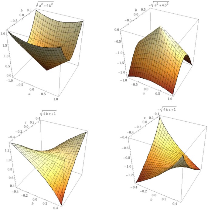
Parametric plot of the eigenvalues of system (2.13). The first row indicates the global minimum, when \(b=c\), while the second row represents the local minimum, when \(a=1, b\neq c\)

Example 3.4
Consider system (2.4), and set
and
Then the solution can be formulated by the integral system of equations, with the initial condition \(\Phi _{0}=0,\Psi _{0}=0\),
Figure 2 presents the behavior of the solution for different values of \(\alpha \in (0,1]\). The behavior of the solution shows the minimax point at the origin. The solution is approximated at the maximum case, when \(\alpha \rightarrow 1\), by

Slope field of solutions of the system (2.4). The solution is approximated at the maximum case, when \(\alpha \rightarrow 1\), where \(\alpha \in (0,1]\), x-axis is Φ and y-axis is Ψ
4 Conclusion
The minimax point theorem is one of the greatest significant consequences of the mathematical analysis theory. It indicates that there is a technique, which together minimizes the maximum loss (sick people) and maximizes the minimum improvement (healthy people). Roughly speaking, there is an approach, which normal people would take supposing the worst-case situation.
Summarizing the above analysis, we have formulated a new mathematical technique based on fractional calculus with the ABC-derivative operator. We formulated a system that satisfies multiple faces of the coronavirus. The total number is suggested as a continuous function of time, which is discrete in the number of faces. We used an approximation method to analyze the system. We recognized that the solution possesses a minimax point. This point indicates the termination of the recent face and realizes a new face of the corona virus.
Availability of data and materials
Data sharing not applicable to this article as no datasets were generated or analyzed during the current study.
References
Djordjevic, J., Silva, C.J., Torres, D.F.M.: A stochastic SICA epidemic model for HIV transmission. Appl. Math. Lett. 84, 168–175 (2018)
Ndairou, F., Area, I., Nieto, J.J., Silva, C.J., Torres, D.F.M.: Mathematical modeling of Zika disease in pregnant women and newborns with microcephaly in Brazil. Math. Methods Appl. Sci. 41(18), 8929–8941 (2018)
Almeida, R., Brito da Cruz, A.M.C., Martins, N., Teresa, M., Monteiro, T.: An epidemiological MSEIR model described by the Caputo fractional derivative. Int. J. Dyn. Control 7(2), 776–784 (2019)
Ibrahim, R.W., Altulea, D.: Controlled homeodynamic concept using a conformable calculus in artificial biological systems. Chaos Solitons Fractals 140, 110132 (2020)
Chen, T.-M., Rui, J., Wang, Q.-P., Zhao, Z.-Y., Cui, J.-A., Yin, L.: A mathematical model for simulating the phase-based transmissibility of a novel coronavirus. Infect. Dis. Poverty 9(1), 1–8 (2020)
Momani, S., Ibrahim, R.W., Hadid, S.B.: Susceptible-infected-susceptible epidemic discrete dynamic system based on Tsallis entropy. Entropy 22(7), 769 (2020)
Ibrahim, R.W.: Perturbed fractional dynamic system of reliability of the evolution and diffusion of viruses. J. Interdiscip. Math., 1–11 (2021)
Baishya, C., Achar, S.J., Veeresha, P., Prakasha, D.G.: Dynamics of a fractional epidemiological model with disease infection in both the populations. Chaos, Interdiscip. J. Nonlinear Sci. 31(4), 043130 (2021)
Akyildiz, F.T., Alshammari, F.S.: Complex mathematical SIR model for spreading of COVID-19 virus with Mittag-Leffler kernel. Adv. Differ. Equ. 2021(1), 319 (2021)
Ahmad, S., Ullah, A., Al-Mdallal, Q.M., Khan, H., Shah, K., Khan, A.: Fractional order mathematical modeling of COVID-19 transmission. Chaos Solitons Fractals 139, 110256 (2020)
Jahanshahi, H., Munoz-Pacheco, J.M., Bekiros, S., Alotaibi, N.D.: A fractional-order SIRD model with time-dependent memory indexes for encompassing the multi-fractional characteristics of the COVID-19. Chaos Solitons Fractals 143, 110632 (2021)
Ibrahim, R.W., Altulea, D., Elobaid, R.M.: Dynamical system of the growth of COVID-19 with controller. Adv. Differ. Equ. 2021(1), 9 (2021)
Aghdaoui, H., Tilioua, M., Nisar, K.S., Khan, I.: A Fractional Epidemic Model with Mittag-Leffler Kernel for COVID-19. Math. Biol. Bioinform. 16(1), 39–56 (2021)
Hadid, S.B., Ibrahim, R.W., Altulea, D., Momani, S.: Solvability and stability of a fractional dynamical system of the growth of COVID-19 with approximate solution by fractional Chebyshev polynomials. Adv. Differ. Equ. 2020(1), 338 (2020)
Askar, S.S., Ghosh, D., Santra, P.K., Elsadany, A.A., Mahapatra, G.S.: A fractional order SITR mathematical model for forecasting of transmission of COVID-19 of India with lockdown effect. Results Phys. 24, 104067 (2021)
Khan, R.A., Gul, S., Jarad, F., Khan, H.: Existence results for a general class of sequential hybrid fractional differential equations. Adv. Differ. Equ. 2021(1), 284 (2021)
Akindeinde, S.O., Okyere, E., Adewumi, A.O., Lebelo, R.S., Fabelurin, O.O., Moore, S.E.: Caputo Fractional-order SEIRP model for COVID-19 epidemic. Alex. Eng. J. (2021)
Atangana, A., Araz, S.I.: Modeling and forecasting the spread of COVID-19 with stochastic and deterministic approaches: Africa and Europe. Adv. Differ. Equ. 2021(1), 57 (2021)
Atangana, A., Araz, S.I.: Mathematical model of COVID-19 spread in Turkey and South Africa: theory, methods, and applications. Adv. Differ. Equ. 2020(1), 659 (2020)
Musa, S.S., Qureshi, S., Zhao, S., Yusuf, A., Mustapha, U.T., He, D.: Mathematical modeling of COVID-19 epidemic with effect of awareness programs. Infect. Dis. Model. 6, 448–460 (2021)
Atangana, A., Araz, S.I.: A novel COVID-19 model with fractional differential operators with singular and non-singular kernels: Analysis and numerical scheme based on Newton polynomial. Alex. Eng. J. 60(4), 3781–3806 (2021)
Atangana, A.: Modelling the spread of COVID-19 with new fractal-fractional operators: can the lockdown save mankind before vaccination? Chaos Solitons Fractals 136, 109860 (2020)
Atangana, A., Araz, S.I.: Modeling third waves of COVID-19 spread with piecewise differential and integral operators: Turkey, Spain and Czechia (2021). medRxiv
Danane, J., Allali, K., Hammouch, Z., Nisar, K.S.: Mathematical analysis and simulation of a stochastic COVID-19 Lévy jump model with isolation strategy. Results Phys. 23, 103994 (2021)
Hussain, G., Khan, T., Khan, A., Inc, M., Zaman, G., Nisar, K.S., Akgul, A.: Modeling the dynamics of novel coronavirus (COVID-19) via stochastic epidemic model. Alex. Eng. J. 60(4), 4121–4130 (2021)
Singh, H., Srivastava, H.M.: Zakia Hammouch, and Kottakkaran Sooppy Nisar. “Numerical simulation and stability analysis for the fractional-order dynamics of COVID-19.”. Results Phys. 20, 103722 (2021)
Shaikh, A.S., Shaikh, I.N., Nisar, K.S.: A mathematical model of COVID-19 using fractional derivative: outbreak in India with dynamics of transmission and control. Adv. Differ. Equ. 2020(1), 373 (2020)
Afzal, A., Ansari, Z., Alshahrani, S., Raj, A.K., Saheer Kuruniyan, M., Saleel, C.A., Nisar, K.S.: Clustering of COVID-19 data for knowledge discovery using c-means and fuzzy c-means. Results Phys. 29, 104639 (2021)
Khajanchi, S., Sarkar, K., Mondal, J., Nisar, K.S., Abdelwahab, S.F.: Mathematical modeling of the COVID-19 pandemic with intervention strategies. Results Phys. 25, 104285 (2021)
Memon, Z., Qureshi, S., Rasool Memon, B.: Assessing the role of quarantine and isolation as control strategies for COVID-19 outbreak: a case study. Chaos Solitons Fractals 144, 110655 (2021)
Caputo, M., Fabrizio, M.: A new definition of fractional derivative without singular kernel. Prog. Fract. Differ. Appl. 1(2), 1–13 (2015)
Atangana, A., Baleanu, D.: New fractional derivatives with nonlocal and non-singular kernel: theory and application to heat transfer model (2016). 1602.03408. arXiv preprint
Ibrahim, R.W., Jahangiri, J.M.: Existence of fractional differential chains and factorizations based on transformations. Math. Methods Appl. Sci. 38(12), 2630–2635 (2015)
Wilson, H.R., Cowan, J.D.: Excitatory and inhibitory interactions in localized populations of model neurons. Biophys. J. 12(1), 1–24 (1972)
Acknowledgements
The authors would like to express their full thanks to the respected editor and reviewers for the deep advise, which improved our paper.
Funding
This research was supported by the Deanship of Scientific Research, Imam Mohammad Ibn Saud Islamic University (IMSIU), Saudi Arabia, Grant No. (21-13-18-056).
Author information
Authors and Affiliations
Contributions
All authors contributed equally and significantly to writing this article. All authors read and agreed to the published version of the manuscript.
Corresponding author
Ethics declarations
Competing interests
The authors declare that they have no competing interests.
Rights and permissions
Open Access This article is licensed under a Creative Commons Attribution 4.0 International License, which permits use, sharing, adaptation, distribution and reproduction in any medium or format, as long as you give appropriate credit to the original author(s) and the source, provide a link to the Creative Commons licence, and indicate if changes were made. The images or other third party material in this article are included in the article’s Creative Commons licence, unless indicated otherwise in a credit line to the material. If material is not included in the article’s Creative Commons licence and your intended use is not permitted by statutory regulation or exceeds the permitted use, you will need to obtain permission directly from the copyright holder. To view a copy of this licence, visit http://creativecommons.org/licenses/by/4.0/.
About this article

Cite this article
Aldawish, I., Ibrahim, R.W. A new mathematical model of multi-faced COVID-19 formulated by fractional derivative chains. Adv Cont Discr Mod 2022, 6 (2022). https://doi.org/10.1186/s13662-022-03677-w
Received:
Accepted:
Published:
DOI: https://doi.org/10.1186/s13662-022-03677-w