
Abstract
In this paper the classification of single traveling wave solutions of \((1+1)\) dimensional Gardner equation with variable coefficients is obtained by applying the complete discrimination system to the polynomial and trial equation methods. In particular, the corresponding solutions for the concrete parameters are constructed to show that each solution in the classification can be realized. Moreover, numerical simulations shown in the paper could help us better understand the nature of each solution.
1 Introduction
Nonlinear differential equations have been widely applied to describe physical phenomena in many scientific fields, such as physics, electronics and other engineering and applied sciences. For hundreds of years, scientists have been studying both the exact and numerical solutions of nonlinear problems [1,2,3,4]. Due to the inaccuracy of numerical solutions, especially when we encounter very sensitive problems such as chaos, exact solutions have important applications. Accurate solutions can also help us better understand physical phenomena and models. Therefore, finding the exact solutions is of great significance.
A shallow water wave (or long wave) is considered a nonlinear dynamic system with wavelength much longer than its depth. It is widely used to describe nonlinear phenomena in the atmosphere and ocean. In order to describe and study the related nonlinear problems, the KdV equation [5] has been established. However, in some situations, the modified KdV equation should be applied when we discuss the effect of surface tension. But in some conditions such as internal solitary waves in a two-layer fluid with surface tension where the KdV and mKdV equation are not valid at some thickness ratios, we need to combine the KdV equation and mKdV, namely study the Gardner equation, which takes the surface tension on solitary waves in a two-layer (stratified) fluid [6] into consideration. The one-dimensional variable-coefficient Gardner equation
where \(a(t)\), \(b(t)\), \(c(t)\) are nonzero arbitrary functions, was proposed to describe internal solitary waves that occur in coastal areas with inhomogeneous media and boundary, such as the northwest continental shelf of Australia and the Baltic Sea [7, 8]. In this paper, the trial equation method [9,10,11,12,13,14] and the complete discrimination system for polynomial method [15,16,17,18,19,20] are applied to the generalized \((1+1)\) dimensional Gardner equation with variable coefficients. In order to ensure the existence of the solutions, the concrete examples of specific parameters are given.
In real life applications, most nonlinear differential equations (or systems of differential equations) contain arbitrary functions of dependent variables and their derivatives. Extensive studies have been conducted by using various numerical and analytical methods for the various forms of equations that emerge. However, these approaches may involve approximate solutions [21]. In recent years, many useful methods have been put forward, such as direct method [22], improved tanh–coth method [23], and so on. However, few methods can get all the traveling wave solutions to the nonlinear equations. So Liu proposed the trial equation method and the complete discrimination system for polynomial method. By these two methods, many difficult problems have been solved [24]. According to [10], we can see that, by taking a special traveling wave transformation
we can actually reduce the nonlinear differential equation with variable coefficients
to the nonlinear ordinary equation
Then, by taking the following trial equation:
and substituting Eq. (5) into Eq. (4), an ordinary equation system is obtained, and the trial function \(F(u)\) could be a polynomial, rational function, or some other irrational function. Upon getting the trial equation, we can obtain the integral form of the original equation as
where \(\xi _{0}\) is an integral constant. Then we can obtain the classification of all traveling wave solutions to Eq. (6). For example, Yang applied Liu’s methods to the Gerdjikov–Ivanov model, and the classification of the single traveling wave solutions was obtained [24].
2 The classification of traveling wave solutions to \((1+1)\) dimensional Gardner equation with variable coefficients
To find the classification of traveling wave solutions to \((1+1)\) dimensional Gardner equation with variable coefficients, we set
where \(\kappa (t)\), \(\omega (t)\) represent nonzero arbitrary functions. Substituting Eq. (7) into Eq. (1) yields
Now we assume that \((\phi ')^{2}\) is equal to a polynomial function, namely
and, via the balance principle, we get \(n=4\), so
Then taking derivatives on both sides of Eq. (10), we have
Substituting (11) into (8), we get
Actually, this system of equations is not solvable. So we must impose some restrictions on it. Setting \(a_{3} = 2b_{1}a_{4}\), where \(b_{1}\) is a constant, we have
So we get \(\kappa (t)=const\), and by setting \(\kappa (t)=\kappa \), we obtain
Let
then Eq. (10) is deformed into
where
So we have
Then the corresponding complete discrimination system is presented as [11]
For the purpose of solving Eq. (24), the solutions of the complete discrimination system of the fourth order polynomial in nine cases are discussed separately.
Case 1. \(D_{4}=0\), \(D_{3}=0\), \(D_{2}=0\). In this case \(G(\varPhi )\) has a root of multiplicity 4, i.e., \(p=0\), \(q=0\), \(r=0\), and then Eq. (20) is presented by
Therefore, by using Eq. (24), we have
where \(\xi _{0}\) is an integral constant. The solutions of Eq. (10) can be shown to be
For example, when \(a_{4}=1\), \(\kappa =-6\), \(b_{1}=1\), \(b(t)=t+1\), we get \(\omega (t)=\frac{1}{2} t^{2}+t+c\), and setting \(c=0\), we can get the solution of Eq. (1) as
Case 2. \(D_{4}=0\), \(D_{3}=0\), \(D_{2}<0\). This time \(G(\varPhi )\) has a pair of conjugate complex roots of multiplicity 2, i.e.,
where \(m>0\). By using Eq. (24), we can obtain
which is a rational solution. So the solutions of Eq. (10) can be shown to be
For instance, when \(a_{4}=1\), \(\kappa =-6\), \(b_{1}=1\), \(b(t)=t+1\), \(p=2\), we have \(\omega (t)=\frac{1}{2} t^{2}+t+c\), and setting \(c=0\), we obtain the solution of Eq. (1) as
Case 3. \(D_{4}=0\), \(D_{3}=0\), \(D_{2}>0\), \(E_{2}=0\). Now \(G(\varPhi )\) has a real root of multiplicity 3 and a real root of multiplicity 1. Thus we have
When \(\varPhi >l\), \(\varPhi >m\) or \(\varPhi < l\), \(\varPhi < m\), the solution of Eq. (24) is
where the expression (35) is a rational solution. So we can obtain the solutions of Eq. (10) as
For example, when \(a_{4}=1\), \(\kappa =-6\), \(b_{1}=1\), \(b(t)=t+1\), we get \(\omega (t)=\frac{1}{2} t^{2}+t+c\), and setting \(l=1\), \(m=-3\), \(c=0\), the solution of Eq. (1) is given by
Case 4. \(D_{4}=0\), \(D_{3}=0\), \(D_{2}>0\), \(E_{2}>0\). Here \(G(\varPhi )\) has two real roots of multiplicity 2, namely
where \(l>m\). When \(\varPhi >l\) or \(\varPhi < m\), we can obtain the solution as
Then we can get the solution of Eq. (10) as
and, when \(m<\varPhi <l\), we have the solution as
Similarly for
For instance, when \(a_{4}=1\), \(\kappa =-6\), \(b_{1}=1\), \(b(t)=t+1\), \(p=-2\), we have \(\omega (t)=\frac{1}{2} t^{2}+t+c\), and setting \(c=0\), and \(\varPhi >1\) or \(\varPhi <-1\), we can get the solution as follows:
Case 5. \(D_{4}>0\) and \(D_{2}>0\), \(D_{3}>0\). This time \(G(\varPhi )\) has four distinct real roots, namely
where \(\alpha _{1}\), \(\alpha _{2}\), \(\alpha _{3}\), \(\alpha _{4}\) are real numbers, and \(\alpha _{1}>\alpha _{2}>\alpha _{3}>\alpha _{4}\). If \(\varPhi >\alpha _{1}\) or \(\varPhi <\alpha _{4}\), then we take the following transformation:
if \(\alpha _{3}<\varPhi <\alpha _{2}\), we similarly use
Substituting (45) or (46) into Eq. (24), we get
where \(m^{2}=\frac{(\alpha _{1}-\alpha _{4})(\alpha _{2}-\alpha _{3})}{( \alpha _{1}-\alpha _{3})(\alpha _{2}-\alpha _{4})}\). By using Eq. (47) and the definition of Jacobi elliptic sine function [25], we have
Combining Eq. (48) with the expressions (45) and (46), we obtain the solution of Eq. (24) with corresponding conditions
thus we have the solution of Eq. (10) as
and
Moreover, we have
where \(m^{2}=\frac{(\alpha _{1}-\alpha _{4})(\alpha _{2}-\alpha _{3})}{( \alpha _{1}-\alpha _{3})(\alpha _{2}-\alpha _{4})}\). Expressions (49)–(52) involve elliptic functions and are double periodic solutions. For example, when \(a_{4}=1\), \(\kappa =-6\), \(b_{1}=1\), \(b(t)=t+1\), we can get \(\omega (t)=\frac{1}{2} t^{2}+t+c\). Setting \(c=0\), if \(p=-5\), \(q=0\), \(r=4\), we have \(\alpha _{1}=2\), \(\alpha _{2}=1\), \(\alpha _{3}=-1\), \(\alpha _{4}=-2\). When \(\varPhi >\alpha _{1}\) or \(\varPhi <\alpha _{4}\), we get the solution
Case 6. \(D_{4}=0\) and \(D_{2}D_{3}<0\). Now \(G(\varPhi )\) has a real root of multiplicity 2 and a pair of conjugate complex roots, i.e.,
where β, l and m are real numbers. By using Eq. (24), we can get
where
Correspondingly we have the solution of Eq. (24) as
hence the solution of Eq. (10) is
which is a solitary wave solution. When \(a_{4}=1\), \(\kappa =-6\), \(b_{1}=1\), \(b(t)=t+1\), \(\beta =1\), \(l=-1\), \(m=2\), we have \(\omega (t)= \frac{1}{2} t^{2}+t+c\), and by setting \(c=0\), we can get the solution of Eq. (1) as
Case 7. \(D_{4}<0\) and \(D_{2}D_{3}\geq 0\). In this case \(G(\varPhi )\) has two distinct real roots and a pair of conjugate complex roots, thus \(G(\varPhi )\) is given by
where β, γ, l, m are real numbers, \(\beta >\gamma \) and \(m>0\). We now use the following transformation:
where
By choosing \(f_{2}>0\) and substituting expression (62) into Eq. (24), we have
where \(m_{2}^{2}=\frac{2}{1+f_{2}^{2}}\). By Eq. (63) and the definition of Jacobi elliptic cosine function [25], we have
Combining expression (63) with (60) leads to the solutions of Eq. (24) given by
Hence we can get the solution of Eq. (10) in the form
where expression (66) involves an elliptic function and is a double periodic solution. For example, when \(a_{4}=1\), \(\kappa =-6\), \(b_{1}=1\), \(b(t)=t+1\), \(\beta =1\), \(\gamma =-1\), \(l=0\), \(m=2\), we have \(a_{2}=3\), \(b_{2}=c_{2}=0\), \(d_{2}=-3\), \(e_{2}=\frac{3}{4}\), \(f_{2}=2\) or \(-\frac{1}{2}\), \(\omega (t)=\frac{1}{2} t^{2}+t+c\). By setting \(f_{2}=2\), \(c=0\), we can obtain the solution of Eq. (1) as
Case 8. \(D_{4}>0\) and \(D_{2}D_{3}\leq 0\). This time \(G(\varPhi )\) has two pairs of conjugate complex roots, namely
where \(\alpha _{1}\), \(\alpha _{2}\), \(l_{1}\) and \(l_{2}\) are real numbers, \(l_{1}\geq l_{2}>0\). We use the transformation
where
and get
where \(m_{2}^{2}=\frac{f_{2}^{2}-1}{f_{2}^{2}}\). By Eq. (71) and the definition of Jacobi elliptic functions, we can obtain
Combining expressions (72) and (73) with (69) yields
and
where
Expression (75) involves elliptic functions and is a double periodic solution. When \(a_{4}=1\), \(\kappa =-6\), \(b_{1}=1\), \(b(t)=t+1\), \(\alpha _{1}=\frac{\sqrt{7}}{2}\), \(\alpha _{2}=-\frac{\sqrt{7}}{2}\), \(l_{1}=3\), \(l_{2}=2\), we have \(\omega (t)=\frac{1}{2} t^{2}+t+c\), \(a_{2}=\frac{7\sqrt{7}}{6}\), \(b_{2}=\frac{29}{2}\), \(c_{2}=- \frac{11}{3}\), \(d_{2}=\sqrt{7}\), \(e_{2}=\frac{5}{3}\), \(f_{2}=3\) and \(\eta =\frac{24\sqrt{23}}{23}\). Setting \(c=0\), we obtain
Case 9. \(D_{4}=0\), \(D_{3}>0\) and \(D_{2}>0\). In this case \(G(\varPhi )\) has two single real roots and a real root with multiplicity 2. We obtain
where \(\alpha _{1}\), \(\alpha _{2}\) and \(\alpha _{3}\) are real numbers, and \(\alpha _{2}>\alpha _{3}\), \(\alpha _{1}=-\frac{\alpha _{2}+\alpha _{3}}{2}\). Denote \(h=(\alpha _{1}-\alpha _{2})(\alpha _{1}-\alpha _{3})\). When \(\varPhi >\alpha _{2}\), \(\alpha _{2}>\alpha _{1}>\alpha _{3}\), we get the solution of Eq. (24) as
thus
When \(\alpha _{1}>\alpha _{2}\) or \(\alpha _{1}<\alpha _{3}\),
and then we have
For instance, if \(a_{4}=1\), \(\kappa =-6\), \(b_{1}=1\), \(b(t)=t+1\), \(p=-9\), \(q=-4\), \(r=12\), then \(\omega (t)=\frac{1}{2} t^{2}+t+c\). Setting \(c=0\), the solution can be obtained as
3 Numerical simulations for modified Gardner equation
In this section, numerical simulations of modified Gardner equation are given. According to the solutions obtained above, each solution is chosen to carry out a typical numerical simulation, using Eqs. (29), (33), (37), (43), (53), (59), (67), (77) and (83). The 3D and the corresponding 2D graphs of are drawn to present the nature of them. In addition, we only focus on the positive one if there is a plus–minus sign in the selected solutions.
-
Case 1. For \(a_{4}=1\), see Fig. 1.
Figure 1 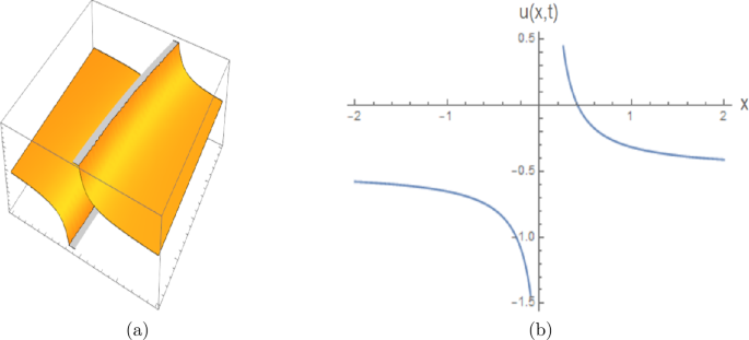
(a) The 3D graph of a rational function solution \(u(x, t)\) appearing in Eq. (29), when \(\kappa =-6\), \(\omega =\frac{1}{2}t^{2}+t\) and \(\xi _{0}=1\); (b) the corresponding 2D graph for \(u(x, t)\), when t = 1
-
Case 2. For \(a_{4}=1\), see Fig. 2.
Figure 2 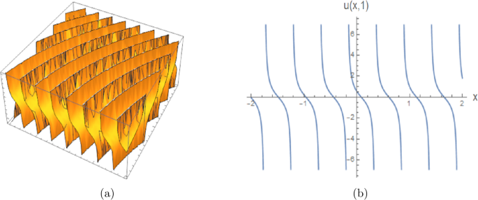
(a) The 3D graph of a triangle function periodic solution \(u(x, t)\) in Eq. (33), when \(\kappa =-6\), \(\omega =\frac{1}{2}t^{2}+t\) and \(\xi _{0}=1\); (b) the corresponding 2D graph for \(u(x, t)\), when t = 1
-
Case 3. For \(a_{4}=1\), see Fig. 3.
Figure 3 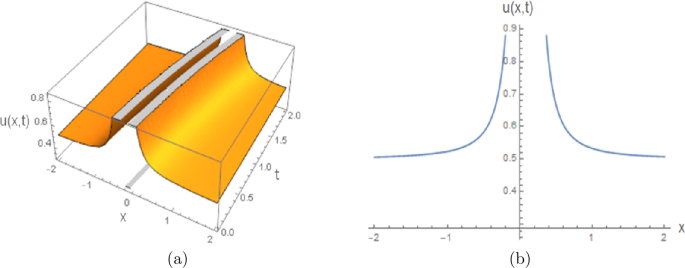
(a) The 3D graph of a rational function solution \(u(x, t)\) illustrating Eq. (37), when \(\kappa =-6\), \(\omega =\frac{1}{2}t^{2}+t\) and \(\xi _{0}=1\); (b) the corresponding 2D graph for \(u(x, t)\), when t = 1
-
Case 4. For \(a_{4}=1\), see Fig. 4.
Figure 4 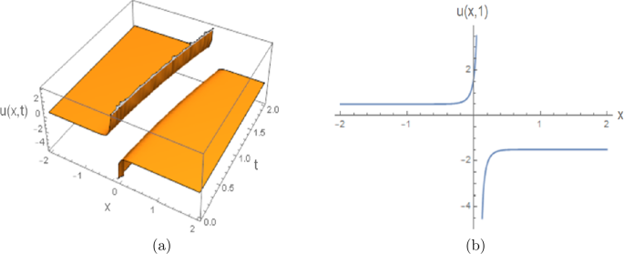
(a) The 3D graph of a hyperbolic cotangent function solution \(u(x, t)\) demonstrating Eq. (43), when \(\kappa =-6\), \(\omega = \frac{1}{2}t^{2}+t\) and \(\xi _{0}=1\); (b) the corresponding 2D graph for \(u(x, t)\), when t = 1
-
Case 5. For \(a_{4}=1\), see Fig. 5.
Figure 5 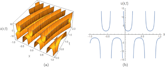
(a) The 3D graph of Jacobi elliptic function solution \(u(x, t)\) appearing in Eq. (53), when \(\kappa =-6\), \(\omega = \frac{1}{2}t^{2}+t\) and \(\xi _{0}=1\); (b) the corresponding 2D graph for \(u(x, t)\), when t = 1
-
Case 6. For \(a_{4}=1\), see Fig. 6.
Figure 6 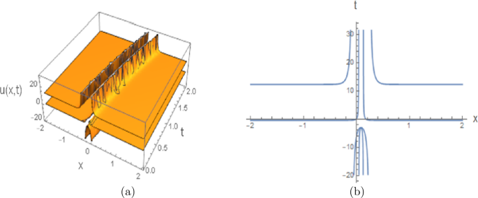
(a) The 3D graph of a solitary wave solution \(u(x, t)\) reflected in Eq. (59), when \(\kappa =-6\), \(\omega =\frac{1}{2}t^{2}+t\) and \(\xi _{0}=1\); (b) the corresponding 2D graph for \(u(x, t)\), when t = 1
-
Case 7. For \(a_{4}=1\), see Fig. 7.
Figure 7 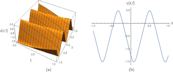
(a) The 3D graph of Jacobi elliptic function solution \(u(x, t)\) illustrating Eq. (67), when \(\kappa =-6\), \(\omega = \frac{1}{2}t^{2}+t\) and \(\xi _{0}=1\); (b) the corresponding 2D graph for \(u(x, t)\), when t = 1
-
Case 8. For \(a_{4}=1\), see Fig. 8.
Figure 8 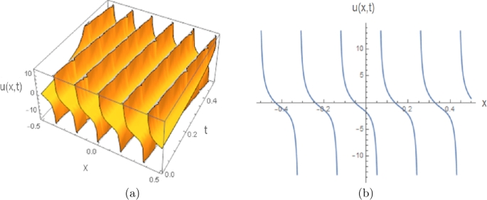
(a) The 3D graph of Jacobi elliptic function solution \(u(x, t)\) demonstrating Eq. (77), when \(\kappa =-6\), \(\omega = \frac{1}{2}t^{2}+t\) and \(\xi _{0}=1\); (b) the corresponding 2D graph for \(u(x, t)\), when t = 1
-
Case 9. For \(a_{4}=1\), see Fig. 9.
Figure 9 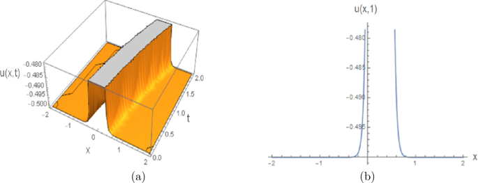
(a) The 3D graph of a solitary wave solution \(u(x, t)\) appearing in Eq. (83), when \(\kappa =-6\), \(\omega =\frac{1}{2}t^{2}+t\) and \(\xi _{0}=1\); (b) the corresponding 2D graph for \(u(x, t)\), when t = 1


4 Conclusion
In this paper, we consider the generalized \((1+1)\) dimensional Gardner equation with variable coefficients. By taking a special traveling wave transformation, the original equation can be changed into the integral form. Then by applying the trial equation method and a complete discrimination system for polynomial method, the classification of the exact solutions is obtained. Moreover, the solitary wave solutions and six kinds of double periodic solutions with Jacobi elliptic functions are given, which are very difficult to get by other methods. In addition, some solutions with the specific parameters are also presented in the paper, thus the existence of the solutions is proved. Our results may be helpful to better understand the two-layer fluid with surface tension, and the problem with specific boundary and initial conditions will be studied in a future work. Moreover, we can also conclude that the trial equation method and the discrimination system for polynomial method are powerful in solving differential equations with variable coefficients arising in mathematical physics.
References
Ablowitz, M.J., Clarkson, P.A.: Solitons, Nonlinear Evolutions and Inverse Scattering. Cambridge University Press, Cambridge (1991)
Liu, C.-S.: Canonical-like transformation method and exact solutions to a class of diffusion equations. Chaos Solitons Fractals 42(1), 441–446 (2009)
Wadati, M.: Invariances and conservation laws of the Korteweg–de Vries equation. Stud. Appl. Math. 59(2), 153–186 (1978)
Bulman, G.W., Sukeyuki, K.: Symmetries and Differential Equations. Springer, New York (1991)
Korteweg, D.J., de Vries, G.: On the change of form of long waves advancing in a rectangular canal, and on a new type of long stationary waves. Philos. Mag. Ser. 5 39, 422–443 (1895)
Ramollo, M.P.: Internal solitary waves in a two-layer fluid with surface tension. Adv. Fluid Mech. 9, 209–219 (1996)
Liu, Y., Gao, Y.-T., Sun, Z.-Y., Yu, X.: Multi-soliton solutions of the forced variable-coefficient extended Korteweg–de Vries equation arisen in fluid dynamics of internal solitary waves. Nonlinear Dyn. 66(4), 575–587 (2011)
Holloway, P.E., Pelinovsky, E., Talipova, T., Barnes, B.: A nonlinear model of internal tide transformation on the Australian North West shelf. J. Phys. Oceanogr. 27(6), 871–896 (1997)
Liu, C.-S.: Trial equation method and its applications to nonlinear evolution equations. Acta Phys. Sin. 54(6), 2505–2509 (2005)
Liu, C.-S.: Using trial equation method to solve the exact solutions for two kinds of KdV equations with variable coefficients. Acta Phys. Sin. 54(10), 4506–4510 (2005)
Liu, C.-S.: Trial equation method to nonlinear evolution equations with rank inhomogeneous: mathematical discussions and its applications. Commun. Theor. Phys. 45(2), 219–223 (2006)
Liu, C.-S.: A new trial equation method and its applications. Commun. Theor. Phys. 45(3), 395–397 (2006)
Liu, C.-S.: Exponential function rational expansion method for nonlinear differential-difference equations. Chaos Solitons Fractals 40(2), 708–716 (2009)
Liu, C.-S.: Trial equation method based on symmetry and applications to nonlinear equations arising in mathematical physics. Found. Phys. 41(5), 793–804 (2011)
Liu, C.-S.: Classification of all single travelling wave solutions to Calogero–Degasperis–Focas equation. Commun. Theor. Phys. 48(4), 601–604 (2007)
Liu, C.-S.: All single travelling wave solutions to Nizhnok–Novikov–Veselov equation. Commun. Theor. Phys. 45(6), 991–992 (2006)
Liu, C.-S.: The classification of travelling wave solutions and superposition of multi-solutions to Camassa–Holm equation with dispersion. Chin. Phys. 16(7), 1832–1837 (2007)
Liu, C.-S.: Representations and classifications of travelling wave solutions to sinh-Gordon equation. Commun. Theor. Phys. 49(1), 153–158 (2008)
Liu, C.-S.: Solution of ODE \(u''+p(u)(u')^{2}+q(u)=0\) and applications to classifications of all single travelling wave solutions to some nonlinear mathematical physics equations. Commun. Theor. Phys. 49(2), 291–296 (2008)
Liu, C.-S.: Applications of complete discrimination system for polynomial for classifications of travelling wave solutions to nonlinear differential equations. Comput. Phys. Commun. 181(2), 317–324 (2010)
Bluman, G.W., Kumei, S.: Symmetries and Differential Equations. Springer, New York (1989)
Hirota, R.: The Direct Method in Soliton Theory. Cambridge University Press, Cambridge (2004)
Sierra, C.A.G., Molati, M., Ramollo, M.P.: Exact solutions of a generalized KdV–mKdV equation. Int. J. Nonlinear Sci. 13(1), 94–98 (2012)
Yang, S.: The envelope travelling wave solutions to the Gerdjikov–Ivanov model. Pramana J. Phys. 91(3), 36–41 (2018)
Wang, Z.-X., Guo, D.-R.: Special Functions. Science Press, Beijing (2002)
Acknowledgements
The authors would like to thank the reviewers for their helpful comments and suggestions to improve the manuscript.
Funding
This work was financed by Grant-in-aid for scientific research from the National Natural Science Foundation of China (NO. 51465047).
Author information
Authors and Affiliations
Contributions
DC and LD worked together in the derivation of the mathematical results. Both authors read and approved the final manuscript.
Corresponding author
Ethics declarations
Competing interests
We would like to declare no conflicts of interest.
Additional information
Publisher’s Note
Springer Nature remains neutral with regard to jurisdictional claims in published maps and institutional affiliations.
Rights and permissions
Open Access This article is distributed under the terms of the Creative Commons Attribution 4.0 International License (http://creativecommons.org/licenses/by/4.0/), which permits unrestricted use, distribution, and reproduction in any medium, provided you give appropriate credit to the original author(s) and the source, provide a link to the Creative Commons license, and indicate if changes were made.
About this article

Cite this article
Cao, D., Du, L. The classification of the single traveling wave solutions to \((1+1)\) dimensional Gardner equation with variable coefficients. Adv Differ Equ 2019, 121 (2019). https://doi.org/10.1186/s13662-019-2061-0
Received:
Accepted:
Published:
DOI: https://doi.org/10.1186/s13662-019-2061-0