
Abstract
In this work, an attempt is made to understand the dynamics of a modified Leslie–Gower model with nonlinear harvesting and Holling type-IV functional response. We study the model system using qualitative analysis, bifurcation theory and singular optimal control. We show that the interior equilibrium point is locally asymptotically stable and the system under goes a Hopf bifurcation with respect to the ratio of intrinsic growth of the predator and prey population as bifurcation parameter. The existence of bionomic equilibria is analyzed and the singular optimal control strategy is characterized using Pontryagin’s maximum principle. The existence of limit cycles appearing through local Hopf bifurcation and its stability is also examined and validated numerically by computing the first Lyapunov number. Optimal singular equilibrium points are obtained numerically for various discount rates.
1 Introduction
The Leslie–Gower model [1, 2] (LG model) shows how asymptotic solutions converge to a stable equilibrium (independent of the initial conditions) state. The equilibrium point depends on the intrinsic factors which govern the system dynamics (in the sense of biology). It marks a significant improvement over the famous Lotka–Volterra model and it is limited in its explanatory capability [3]. Korobeinikov [4] established the global stability of a positive equilibrium point and showed that the limit cycle could be admitted by the model system. This limit cycle also exists if we take the Holling type-II or -III functional response. Aziz and Okiye [5] have designed and studied the modified LG model with cyrtoid type functional response. Huang and Xiao [6] investigated a predator–prey system with Holling type-IV functional response. The qualitative analysis and bifurcation theory along with numerical simulations indicated that it has a unique stable limit cycle. Yafia et al. [7] studied the limit cycle in a modified LG model with Holling type-II scheme bifurcated from small and large time delays. Ji et al. [8] extended the study of the modified LG model designed by Aziz and Camara for stochastic perturbation. Huang et al. [9] studied controlling bifurcation in a delayed fractional predator–prey system with incommensurate orders. Rihan et al. [10] investigated fractional-order delayed predator–prey systems with Holling type-II functional response. Song et al. [11] have studied dynamic analysis of a fractional-order delayed predator–prey system with harvesting. Xu et al. [12] studied the stability and Hopf bifurcation of a population model with Holling type-IV functional response and time delay. Jana et al. [13] have studied a hybrid type tri-trophic food chain model (Holling type-IV and Beddington–DeAngelis type functional responses) and try to understand the role of top predator interference and gestation delay and observed the subcritical Hopf bifurcation phenomena in the designed model system and the bifurcating periodic solution is unstable for the considered set of parameter values. Yu [14] studied the global stability of a modified LG model with Beddington–DeAngelis type functional response. Recently, Agrawal et al. [15] investigated the occurence of double Hopf bifurcation at positive equilibrium point when they choose appropriate measure of the tolerance of the prey. Furthermore, some dynamic behaviors, such as stability switches, chaos, bifurcation and double Hopf bifurcation scenarios are observed using numerical simulations.
Presently, the population dynamics is a very importance topic in the field of bio-economics and related to the optimal management of renewable resources. It is more realistic to introduce the harvesting factor in the model system. We also introduce the idea of maximal sustainable yield in the management of renewable resources. It suggests exploiting the surplus production on the basis of biological growth model. Clark [16] reviewed how harvesting affects the fisheries management using ecological and economic models. Hoekstra et al. [17] studied the conservation and harvesting of a population dynamic model system and illustrated that several types of optimal harvesting solutions are possible and depend on both ecological parameters such as the predators search and handling time of prey and economic parameters (e.g., the maximum harvest rate, the discount rate and the cost of fishing). We know that mainly three types of harvesting have been reported in the literature: (i) constant rate of harvesting, (ii) proportional harvesting \(h(x)=qEx\), where q is the catch ability coefficient, E is the effort made for harvesting and the product qE is the fishing mortality [18], and (iii) nonlinear harvesting \(h(x)=qEx/(m_{1}E+m_{2}x)\), where \(m_{1}\) and \(m_{2}\) are suitable positive constants, proportional to the ratio of the stock level to the harvesting rate at high levels of effort and to the ratio of the effort level to the harvesting rate at high stock levels, respectively. Azar et al. [19] studied the Lotka–Volterra type two prey one predator model where the predator is harvested with two different schemes: (i) constant harvesting quota and (ii) constant harvesting effort, and one reported that a constant harvesting quota on the predator may destabilize the system. Zhu and Lan [20] made a Hopf bifurcation analysis of the LG model with constant prey harvesting. The dynamics of a model with proportionate harvesting has been studied by Mena-Lorca et al. [21]. Zhang et al. [22] studied the harvested LG model and found that harvesting has no influence on the persistence of the model system. So, the predator density strictly decreases with harvesting effort but it has no effect on the prey density. Kar and Ghorai [23] analyzed the dynamics of a delayed predator–prey model with harvesting in a modified LG model. Gupta et al. [24] studied the bifurcation analysis and control of the LG model with Michaelis–Menten type prey harvesting and observed that for a wide range of initial values the system goes to extinction. Recently, Huang et al. [25] studied the effect of constant yield predator harvesting on the dynamics of a LG model. The model exhibits different types of bifurcations including the saddle-node bifurcation, attracting and repelling Bogdanov–Takens bifurcations, and all types of Hopf bifurcation with the variation of the control parameters. Saleh [26] studied the dynamics of a modified LG model with quadratic predator harvesting.
We have proposed a new 2D modified Leslie–Gower type predator–prey model with Holling type-IV functional response in this manuscript. We have also incorporated the nonlinear harvesting in the prey population. Andrews [27] explored a function of the form \(f(x)=mx/((x^{2}/i)+x+a)\) and named it the Holling type-IV functional response or Monod–Haldane [28] function, which is similar to the Monod (i.e., the Michaelis–Menten) function for low concentration but includes the inhibitory effect at high concentrations. The parameters m and a can be interpreted as the maximum per capita predation rate and the half saturation constant in the absence of any inhibitory effect. The parameter i is a measure of the predator’s immunity from or tolerance of the prey. We have analyzed this model for its rich dynamics and studied the bio-economic equilibria using singular optimal control strategies.
This work is organized as follows. In the next section, model formulation and biological meaning of the parameters are given. In Sect. 3, we presented the detail analysis of the model system. In Sect. 4, we discuss the linear stability analysis and Hopf bifurcation. Stability of the limit cycle is also presented in this section. Section 5 discusses the bionomic equilibria and optimal harvesting policy. In Sect. 6, some numerical simulation results are presented to illustrate or complement our mathematical findings. Conclusions and discussions are given in the final section which summarizes our findings.
2 Model formulation
The Leslie–Gower type model described [29] in extended form is given by
subject to positive initial condition \(u(0)>0\), \(v(0)>0\). Here \(u\equiv u(t)\) and \(v\equiv v(t)\) are the prey and predator population density, respectively.
Model system (1) is defined on the set
with all the parameters r, K, m, i, s, a and n being positive. Further, the biological meanings of the parameters are listed in Table 1.
The interaction between prey and predator is expressed by a Holling type-IV functional response, that is, \(f(u)= \frac{mu}{\frac{u^{2}}{i}+u+a}\) [3]. Taylor [30] has suggested that the subsistence of the predator depends on prey population therefore, the conventional environmental carrying capacity \(K_{v}\) of the predator is taken to be proportional to the prey abundance u, thus \(K_{v}= \frac{u}{n}\).
2.1 The model with prey harvesting
We introduce the nonlinear harvesting \(H(u)= \frac{qEu}{m_{1} E+m_{2} u}\) in the model system (1). Therefore the modified system of differential equations is
subject to the positive initial condition \(u(0)=u_{0}>0\) and \(v(0)=v_{0}>0\). The parameter r, K, m, i, s, a and n have the same biological meaning as in model (1), q is the catchability coefficient, E is the effort made to harvest individuals and \(m_{1}\), \(m_{2}\) are suitable constants. All parameter are assumed to be positive. System (3) is defined on the set Ω.
We introduce the following substitutions to bring the system of equations into non-dimensional form:
The constants \(m_{1}\), \(m_{2}\) are chosen in such a way that \((\frac{m_{1}}{m_{2}})E< u\) where u is the prey biomass at a given instant of time. The model system takes the following form:
subject to the initial condition
Here,
and α, β, γ, δ, h and c are positive constants.
3 Analysis of the model system
3.1 Positivity and boundedness of solution
Lemma 1
(a) All solutions \((x(t), y(t))\) of system (4) with the initial condition (5) are positive for all \({t\geq 0}\). (b) All solutions \((x(t),y(t))\) of system (4) with the initial condition (5) are bounded for all \({t\geq 0}\).
Proof
(a) Integrating Eq. (4) with initial condition (5) we have
Hence the whole solution starting in \(\operatorname {Int}(\Omega )=\{(x, y)\in R^{2}|x>0, y>0\}\) remains in \(\operatorname {Int}(\Omega )\) for all \(t\geq 0\). Since the trajectories which start in positive direction of the x-axis and remain on it at all future time, the positive x-axis is an invariant set and similarly the positive y-axis is an invariant set for the system (4). Combining the two we observe that the set Ω defined in (2) is an invariant set for system (4).
(b) To prove the boundedness of solutions of Eq. (4), we use the positivity of variables x, y and results of Lin and Ho [31]. From (4) we can write
which gives
Therefore,
Further, from Eq. (4) we have
which gives
Therefore, \(y(t)\leq \max\{\frac{M_{1}}{\beta }, y_{0}\}\equiv M_{2}\). This completes the proof of the boundedness of solutions and hence the system under consideration is a dissipative system. □
3.2 Equilibrium analysis
To find the equilibrium points of the model system (4), we need to study the zero growth isoclines and the point of interaction. The equilibrium points of system (4) are obtained by
The axial equilibrium points are given by the roots of the quadratic equation,
and the interior equilibria are given by the roots of the following bi-quadratic equation:
where \(P=\beta \), \(Q=\beta (\alpha +c-1)\), \(R=\alpha \beta c-c\beta + \alpha +h\beta +\alpha \beta \gamma -\alpha \beta \), \(S=\alpha (c+ \beta h-\beta \gamma +c\beta \gamma -c\beta )\) and \(T=\alpha \beta \gamma (h-c)\).
The roots of Eqs. (8) and (9) depend on the parameters h and c, so we shall consider the following cases.
Case I. When \(h>c\)
Axial Equilibria
The possible equilibrium points on the boundary of the first quadrant for system (4) are \(E_{1}=(x_{1}, 0)\), \(E_{2}=(x_{2}, 0)\) where \(x_{1}\), \(x_{2}\) are the positive real roots of the quadratic equation (8) with \(x_{1}< x_{2}\) and are given by
The two real positive roots \(x_{1}\) and \(x_{2}\) will exist if \(c<1\) and \((1+c)^{2}-4h>0\). Note that the other cases are not biologically feasible.
Interior Equilibria
From (9), it is obvious that \(P>0\) and \(T>0\). If either (i) \(Q, R, S<0\), or (ii) \(Q, S>0\), \(R<0\), or (iii) \(Q<0\), \(S, R>0\), or (iv) \(Q, R>0\), \(S<0\), or (v) \(Q>0\), \(S, R<0\), or (vi) \(Q, R<0\), \(S>0\), then by Descartes’ rule Eq. (9) has either two positive real roots or no real root and if either \(Q, S<0\), \(R>0\), then by Descartes’ rule Eq. (9) has either four positive real root or two positive real roots or no real root. Note that the other cases are not biologically feasible.
Case II. When \(h< c\)
Axial Equilibria
In this case \(x=\tilde{x}\) is the only positive real root of Eq. (8). For \(h< c\), the product of roots is negative. Therefore, the two roots are either of opposite sign or complex conjugates. The root \(\tilde{x}=\frac{(1-c)+\sqrt{(1+c)^{2}-4h}}{2}\) and the real positive root x̃ will exist if \(c<1\) and \((1+c)^{2}-4h>0\). Hence the axial equilibria are \(\tilde{E}=( \tilde{x}, 0)\).
Interior Equilibria
From Eq. (9), obviously \(P>0\) and \(T<0\). If either (i) \(Q, R, S<0\), or (ii) \(Q, R, S>0\), then by Descartes’ rule Eq. (9) has only one positive real root and if either (i) \(Q>0\), \(R>0\), \(S<0\), or (ii) \(Q>0\), \(R<0\), \(S>0\), or (iii) \(Q<0\), \(R<0\), \(S>0\), or (iv) \(Q<0\), \(R>0\), \(S<0\), or (v) \(Q>0\), \(R<0\), \(S<0\), or (vi) \(Q<0\), \(R>0\), \(S>0\), then by Descartes’ rule Eq. (9) has either three positive real roots or one positive real root. Note that the other cases are not biologically feasible.
Case III. When \(h=c\)
Axial Equilibria
In this case \(x=1-c\) is the only positive real root of Eq. (8). Therefore the axial equilibrium point is \(E=(1-c, 0)\) provided \(c<1\).
Interior Equilibria
From Eq. (9), it is obvious that \(P>0\). If either (i) \(Q, R, S<0\), or (ii) \(Q>0\), \(R<0\), \(S<0\), or (iii) \(Q>0\), \(R>0\), \(S<0\), then by Descartes’ rule Eq. (9) has only one positive real root and if either \(Q<0\), \(R>0\), \(S<0\), then by Descartes’ rule Eq. (9) has either three positive real roots or one positive real root and if either (i) \(Q>0\), \(R<0\), \(S>0\), or (ii) \(Q<0\), \(R>0\), \(S>0\), or (iii) \(Q<0\), \(R<0\), \(S>0\), then by Descartes’ rule Eq. (9) has either two positive real roots or no positive real root. Note that the other cases are not biologically feasible.
4 Linear stability analysis and Hopf bifurcation
Theorem 1
-
(a)
For \(h>c\), the axial equilibrium point \(E_{1}=(x_{1}, 0)\) is a repeller and \(E_{2}=(x_{2}, 0)\) is a saddle point.
-
(b)
For \(h< c\), the axial equilibrium point \(\tilde{E}=(\tilde{x}, 0)\) is always a saddle point.
-
(c)
For \(h=c\), the axial equilibrium point \(E=(1-c, 0)\) is always a saddle point.
Proof
The Jacobian of system (4) evaluated at a point \((x, 0)\) is
The eigenvalues of the Jacobian matrix are \(1-2x-\frac{hc}{(c+x)^{2}}\) and δ.
-
(a)
For the equilibrium point \(E_{1}=(x_{1}, 0)\), the eigenvalues \(1-2x-\frac{hc}{(c+x)^{2}}\) and δ are both positive and so the equilibrium point \(E_{1}\) is a repeller. Similarly at the equilibrium point \(E_{2}=(x_{2}, 0)\), the eigenvalue \(1-2x-\frac{hc}{(c+x)^{2}}\) and \(\delta >0\) and the equilibrium point \(E_{2}\) is a saddle point.
-
(b)
Since \(\tilde{E}=E_{2}\), Ẽ is saddle point.
-
(c)
For the axial equilibrium point \(E=(1-c, 0)\), the eigenvalues are \(1-2x-\frac{hc}{(c+x)^{2}}=-(1-c)^{2}<0\) and \(\delta >0\) and the equilibrium point E is a saddle point.
□
Theorem 2
-
(a)
The equilibrium point \(E_{*}(x_{*}, y_{*} )\) (for all three cases) is locally asymptotically stable if \(\frac{1}{2}< x_{*}<\sqrt{\alpha \gamma }\).
-
(b)
System (4) undergoes a Hopf bifurcation with respect to the bifurcation parameter \(\delta =\tilde{\delta }\) around the equilibrium point \(E_{*} (x_{*}, y_{*})\) if \(x_{*}>\frac{1}{2}\) and \(\alpha \beta \tilde{\delta }(\frac{x^{2}}{\alpha }+x+\gamma )^{2}= \alpha (\frac{x^{2}}{\alpha }+x+\gamma )[\beta (1-2x_{*})(x_{*}+c)(\frac{x ^{2}}{\alpha }+x+\gamma )-c\beta (1-x_{*})(\frac{x^{2}}{\alpha }+x+ \gamma )+cx_{*}]-x_{*}(\alpha \gamma -x_{*}^{2}\beta )(x_{*}+c)\).
The proof is given in Appendix A1.
Theorem 3
System (4) undergoes a saddle-node bifurcation around \(E_{*}(x_{*}, y_{*})\) with respect to the bifurcation parameter h if:
-
(i)
\(2\beta x_{*}^{5}+\beta (4\alpha +c-1)x_{*}^{4}+\alpha \beta (2c+2 \alpha -2+4\gamma )x_{*}^{3} +\alpha (2c\beta \gamma -\beta +c\alpha \beta +\alpha -c+4\alpha \beta \gamma -\beta \gamma )x_{*}^{2} +(c \beta \gamma -\beta +2\beta \gamma^{2}-\beta \gamma +2\gamma )x_{*}+ \alpha^{2}(\beta c\gamma +\beta \gamma +c\gamma )=0\),
-
(ii)
\(2\beta x_{*}^{6}+\beta (4\alpha +c-1+\delta )x_{*}^{5}+(2c \alpha \beta +2\alpha^{2}\beta +2\alpha \beta \delta -\alpha +2\alpha \beta \gamma +c\beta \delta +2\alpha \beta \gamma -2\alpha \beta )x _{*}^{4} +\alpha (2c\beta \gamma +c\beta -\beta \gamma -\beta -2c+c \alpha \beta +4\alpha \beta \gamma -\alpha \beta +\alpha \beta \delta -2c\beta \delta )x_{*}^{3} +\alpha (2c\alpha \beta \gamma -2\alpha \beta \gamma -c\alpha +\alpha \beta \gamma^{2}+2\alpha \beta \gamma \delta +\alpha \gamma +2c\beta \gamma \delta +c\alpha \beta \delta )x _{*}^{2} +\alpha^{2}\beta (c\gamma^{2}+\gamma^{2}\delta +2c\gamma \delta -\gamma^{2})x_{*}+c\alpha^{2}\beta \gamma^{2}\delta >0\), and
-
(iii)
\(\sqrt{\frac{\alpha \gamma }{3}}< x_{*}<(2hc)^{1/3}-c\).
The proof is given in Appendix A2.
4.1 Stability of limit cycles
Following Perko [32], we now compute the Lyapunov coefficient σ at the point \(E_{*}(x_{*}, y_{*})\) of system (4) to discuss the stability of the limit cycle. Let us translate the equilibrium \(E_{*}(x_{*}, y_{*})\) of system (4) to the origin by using the transformation \(\tilde{x}=x-x_{*}\) and \(\tilde{y}=y-y _{*}\). Then system (4) in a neighborhood of the origin can be written as
Now
where \(F^{1}(\tilde{x}, \tilde{y})\) and \(F^{2}(\tilde{x}, \tilde{y})\) are power series in powers of \(\tilde{x}^{i}\tilde{y}^{j}\) satisfying \(i+j>4\). Then we obtain
where
with \(F^{1}(\tilde{x}, \tilde{y})=\sum_{i+j=4}^{\infty }a_{ij} \tilde{x}^{i}\tilde{y}^{j}\) and \(F^{2}(\tilde{x}, \tilde{y})=\sum_{i+j=4} ^{\infty }b_{ij}\tilde{x}^{i}\tilde{y}^{j}\). Hence the first Lyapunov coefficient σ for the planar system is given by
where
Since the expression for the Lyapunov number σ is complicated we cannot say anything about the sign of σ and therefore we have analyzed it numerically.
5 Bionomic equilibria
The bionomic equilibrium is obtained when the total revenue obtained by selling the harvested biomass equals the total cost utilized in harvesting. The net profit at any time [33] is given by
Note that if the harvesting cost is greater than the revenue for prey species (i.e. \(C>\frac{pqx}{m_{1}E+m_{2}x}\)), then the harvesting in prey species is not profitable and it is of no interest. Hence, we consider that the cost must be less than the revenue for prey species (i.e. \(C<\frac{pqx}{m_{1}E+m_{2}x}\)).
The bionomic equilibrium \((x, y,E)\) is given by the positive solutions of \(\frac{dx}{dt}=\frac{dy}{dt}=P=0\). That is,
Thus, the bionomic equilibria are the points of intersection of biological equilibrium line and zero profit line. Solving Eqs. (12) and (13), we obtain the value of \(x_{\infty }\) and \(y_{\infty }\) and from (14) we obtain \(E_{\infty }=\frac{pq-Cm_{2}}{cm_{1}}x_{\infty }\) if \(Cm_{2}< pq\).
5.1 Optimal harvesting policy
In this section, we explain the optimal harvesting policy or singular optimal control to be adopted by a regulatory agency. With the help of Pontryagin’s maximum principle [34], we maximize the current value of the continuous time stream of revenues, which is given by
where μ denotes the continuous annual discount rate which is fixed by harvesting agencies. The control variable E is subject to the constraint \(0\leq E\leq E_{m}ax\), where \(E_{m}ax\) is a feasible upper limit for the harvesting effort.
Therefore, the optimal control problem over an infinite time horizon is given by
subject to Eqs. (3) with \((x, y)\neq (0, 0)\) and \(x(0)=x_{0}\), \(y(0)=y_{0}\).
The Hamiltonian function is given by
where \(\lambda_{i}=\lambda_{i}(t)\), \(i=1, 2\), are adjoint variables.
Differentiating the Hamiltonian H with respect to the control variable E, we get
The considered control problem admits a singular solution on the control set \([0,E_{\max}]\), if \(\frac{\partial H}{\partial E}=0\), which gives
where \(\lambda_{1}e^{\mu t}\) is the usual shadow price [30].
In order to find the path of a singular control, Pontryagin’s maximum principle [34] is utilized and the adjoint variables must satisfy the adjoint equations given by
For a singular optimal equilibrium solution, we use the steady state equations (12) and (13) in terms of \(x^{*}\) and \(y^{*}=\frac{x^{*}}{n}\), hence \(x^{*}\), \(y^{*}\) and E can be taken as constant [35]. Thus Eq. (19) along with the steady state equations (12) and (13) give
Due to the presence of the term \(e^{-\mu t}\), no steady state is possible for the above system. Following Srinivasu et al. [36], we consider the transformation
where \(\tau_{i}\) represents the present value of the adjoint variable \(\lambda_{i}\). Using Eq. (18), Eq. (21) can be written in terms of \(\tau_{2}\) as follows:
where
This shadow price \(\tau_{i}(t)=\lambda_{i}(t)e^{-\mu t}\), \(i=1,2\), should remain constant over time in singular equilibrium to satisfy the transversality conditions at ∞ (i.e. \(\lim_{t\rightarrow \infty }\lambda_{i}(t)=0\) for \(i=1,2\)). Thus, the solution of Eq. (23) satisfying the transversality condition for the discounted autonomous infinite horizon problem (16) is \(\tau_{2}=\frac{R(x ^{*})}{(s+\mu )}\).
Using the above value of \(\tau_{2}\) Eq. (20) can be written in terms of \(\tau_{1}\) as follows:
where
The solution of Eq. (23) satisfying the transversality condition at ∞ is given by
From Eqs. (18) and (24) we obtain
This gives the desired singular path.
Equation (25) along with the steady state equations (12) and (13) reduces to the following polynomial equation in \(x^{*}\):
where \(A_{1}\), \(A_{2}\), \(A_{3}\), \(A_{4}\), \(A_{5}\), \(A_{6}\) are found using MATHEMATICA and are given by
Equation (26) will have at least one positive real root for \(x^{*}\) if \(A_{1}>0\) and \(A_{6}<0\). Equivalently, we can say that if \(m_{2}C>pq\) and \(G>aEH\), then Eq. (26) will have at least one positive real root for \(x^{*}\), which together with the steady state equations (12) and (13) gives the singular equilibrium point
Notice that
and
Therefore, in the case of singular control (i.e. \(\frac{\partial H}{ \partial E}=0\))
for all \(t\in [0, \infty )\) provided
and \(\lambda_{i}(t)\), \(i=1, 2\) are positive i.e. \(R(x^{*} )>0\) and \(\xi (x^{*})+\mu >0\), which gives
Thus, the maximized Hamiltonian \(H^{*}\) is concave in both x and y for all \(t\in [0, \infty )\) provided (27) and (28) are satisfied. Hence, the Arrow sufficiency condition for an infinite time horizon is satisfied [34] under certain constraints.
The generalized Legendre–Clebsch condition for the optimal control problem (16) is trivially satisfied as \(\frac{\partial H}{\partial E}=0\) for all \(t\in [0, \infty )\) along the optimal singular solution. Hence, from the Arrow sufficient conditions for infinite time horizon and generalized Legendre–Clebsch condition, the singular solution \((x^{*},y^{*},E^{*})\) is a part of the optimal solution (piecewise continuous curve) locally.
Further, by differentiating (17) with respect to t along a singular solution together with \(\frac{dx}{dt}=0\) and \(\frac{d \lambda_{1}}{dt}=\frac{-\mu \eta (x)}{\xi (x)+\mu }e^{-\mu t}\), we obtain
for all \(t\in [0, \infty )\).
From (29), we infer that the singular optimal solution is \((x^{*}, y^{*}, E^{*})\) where \(x^{*}\), the positive root of the equation, is
which coincides with Eq. (25) for the singular solution. The maximum present value can be found by the evaluation of the performance measure in the obtained optimal values from the previous analysis [37]. In this case
This gives
Therefore
The transversality condition is
and it is trivially satisfied. This result agrees with the Michel theorem for the discounted autonomous infinite horizon model [38].
6 Numerical simulation results
The model system (4) is integrated numerically using the Runge–Kutta method for different sets of parameters values.
-
(i)
For \(\alpha =0.1\), \(\beta =2\), \(c=0.004\), \(\delta =0.5\), \(\gamma =1\), \(h=0.09\), the equilibrium points are \(E_{1}(0.101018, 0.050509)\) and \(E_{2}(0.847354, 0.423677)\).
For the equilibrium point \(E_{1}(0.101018, 0.050509)\), \(\operatorname {Tr}N=0.233986\) and \(\det N=-0.346001\). For the equilibrium point \(E_{2}(0.847354, 0.423677)\), \(\operatorname {Tr}N=-1.16308\) and \(\det N=0.355004\). The equilibrium point \(E_{1}(0.101018, 0.050509)\) is a saddle point and the equilibrium point \(E_{2}(0.847354, 0.423677)\) is a stable focus, which is shown in Fig. 1.
Figure 1 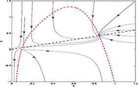
The prey and predator nullclines are represented by red and blue lines respectively. The equilibrium point \(E_{1} (0.101018,0.050509)\) is saddle point and the equilibrium point \(E_{2}(0.847354,0.423677)\) is stable focus
-
(ii)
For \(\alpha =0.2\), \(\beta =0.125\), \(c=0.049\), \(\delta =0.12\), \(\gamma =1\), \(h=0.05\), which gives the two equilibrium point \(E_{11}(0.0018, 0.0144)\) and \(E_{21}(0.0695, 0.556)\).
The equilibrium point \(E_{11}(0.0018, 0.0144)\) is a saddle point as the eigenvalues of Jacobian matrix are −0.107753 and 0.0208392. A stable limit cycle appears in a small neighborhood of \(E_{21}(0.0695, 0.556)\) as the Lyapunov number \(\sigma =-30387.3\pi <0\) (see Fig. 2).
Figure 2 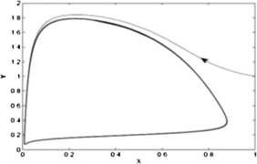
The figure shows that the limit cycle around the equilibrium point \(E_{21} (0.0695,0.556)\) is stable
-
(iii)
For \(\alpha =0.5\), \(\beta =7.5\), \(c=0.1\), \(\delta =0.002\), \(\gamma =1\), \(h=0.05\), we have only one equilibrium point, \(E_{*}(0.9169, 0.1223)\).
For the equilibrium point \(E_{*}(0.9169, 0.1223)\), \(\operatorname {Tr}N=-0.8342\) and \(\det N=0.0017\) and so the equilibrium point \(E_{*}(0.9169, 0.1223)\) is a stable focus, which is shown in Fig. 3.
Figure 3 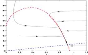
The prey and predator nullclines are represented by red and blue lines respectively. The equilibrium point \(E^{*}(0.9169,0.1223)\) is stable focus
-
(iv)
For \(\alpha =0.2\), \(\beta =0.125\), \(c=0.1\), \(\delta =0.12\), \(\gamma =1\), \(h=0.05\), the equilibrium point is \(E_{*}(0.09177, 0.73416)\).
An unstable limit cycles appears in a small neighborhood of \(E_{*}(0.09177, 0.73416)\) as the Lyapunov number \(\sigma =728.498 \pi >0\) (see Fig. 4).
Figure 4 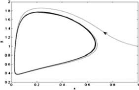
The figure shows that the limit cycle around the equilibrium point \(E_{*}(0.09177, 0.73416)\) is unstable
-
(v)
For \(\alpha =0.5\), \(\beta =7.5\), \(c=0.1\), \(\delta =0.002\), \(\gamma =1\), \(h=0.1\), we have only one equilibrium point, which is \(E^{**}(0.8617, 0.1149)\).
For the equilibrium point \(E^{**}(0.8617, 0.1149)\), \(\operatorname {Tr}N=-0.7312\) and \(\det N=0.0015\), so the equilibrium point \(E^{**}(0.8617, 0.1149)\) is a stable focus, which is shown in Fig. 5.
Figure 5 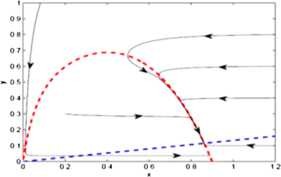
The prey and predator nullclines are represented by red and blue lines respectively. The equilibrium point \(E^{**}(0.8617,0.1149)\) is stable focus
-
(vi)
For \(\alpha =0.2\), \(\beta =0.125\), \(c=0.01\), \(\delta =0.12\), \(\gamma =1\), \(h=0.01\), the equilibrium point is \(E_{3}(0.1196, 0.9568)\).
An unstable limit cycles appears in a small neighborhood of \(E_{3}(0.1196, 0.9568)\) as the Lyapunov number \(\sigma =330.29\pi >0\) (see Fig. 6).
Figure 6 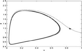
The figure shows that the limit cycle around the equilibrium point \(E_{3}(0.1196, 0.9568)\) is unstable


Also it is too difficult to solve Eq. (26) analytically and therefore we consider the following numerical examples.
- Case (i) :
-
For \(h>c\): For the parameters \(a=1\), \(n=1\), \(m=0.4\), \(s=0.01\), \(r=0.02\), \(i=0.1\), \(p=0.5\), \(q=0.9\), \(K=100\), \(C=0.03\), \(m_{1}=0.1\), \(m_{2}=0.03\), the optimal singular solutions for different rates of μ are given in Table 2.
Table 2 Optimal singular solution for different discount rate μ - Case (ii) :
-
For \(h< c\): For the parameters \(a=1\), \(n=1\), \(m=0.4\), \(s=0.01\), \(r=0.02\), \(i=0.1\), \(p=0.5\), \(q=0.0009\), \(K=100\), \(C=0.03\), \(m_{1}=0.1\), \(m_{2}=0.03\), the optimal singular solutions for different rates of μ are given in Table 3.
Table 3 Optimal singular solution for different discount rate μ - Case (iii) :
-
For \(h=c\): For the parameters \(a=1\), \(n=1\), \(m=1.04\), \(s=0.1\), \(r=0.02\), \(i=0.9\), \(p=0.5\), \(q=0.002\), \(K=100\), \(C=0.003\), \(m_{1}=0.1\), \(m_{2}=0.03\), the optimal singular solutions for different rates of μ are given in Table 4.
Table 4 Optimal singular solution for different discount rate μ
Note that \(y_{(j)}^{*}=x_{(j)}^{*}\), \(j=1,2,3,4,5\), since in each case \(n=1\).
It is clearly seen that we can find an optimum equilibrium for various discount rates μ in various cases. From the above tables we conclude that there is at least one optimum singular equilibrium point in each from which \((x_{(1)}^{*},y_{(1)}^{*},E_{(1)}^{*})\) is feasible from an ecological point of view. Once the optimal singular solution is known then one can easily find the optimal paths (see Figs. 7–9).

Plot \(E^{*}\) vs \(x^{*}\) for the case (i) with \(\mu= 0.2\)

Plot \(E^{*}\) vs \(x^{*}\) for the case (ii) with \(\mu=0.2\)

Plot \(E^{*}\) vs \(x^{*}\) for the case (iii) with \(\mu= 0.2\)
7 Conclusions and discussions
In this paper, a mathematical model to study the dynamical behavior of a modified Leslie–Gower model with Holling type-IV functional response and nonlinear prey harvesting has been proposed and analyzed. The existence of equilibrium points and their stability analysis have been discussed with the help of stability theory. The proposed model system undergoes a Hopf bifurcation and a saddle-node bifurcation around the equilibrium point for the control parameter δ, the ratio of intrinsic growth rates of the predator and prey population and \(h=\frac{qE}{rm_{2}K}\), respectively.
We have discussed the bionomical equilibrium of the model and explain the optimal harvesting policy to be adopted by a regulatory agency. By constructing an appropriate Hamiltonian function and using Pontryagin’s maximum principle, the optimal harvesting policy has been discussed. We also found an optimal equilibrium solution. The effect of harvesting the prey, predator or both on the stability of the system depends on a pretty fine-tuned balancing of the parameter values and also on which functions/functional responses are chosen to represent the ecological harvesting policy [39]. We have established the stability of a limit cycle using the first Lyapunov number around the equilibrium point. A stable limit cycle seems to be possible only when the per capita consumption of prey by the predator is bounded by some maximum value, as with the nonlinear prey harvesting. Optimal singular equilibrium points have been obtained numerically for various discount rate in various cases. Therefore, at least one optimum singular equilibrium point in each from which \((x_{(1)}^{*}, y_{(1)}^{*}, E_{(1)}^{*})\) is feasible from an ecological point of view.
References
Leslie, P.H., Gower, J.C.: The properties of a stochastic model for the predator–prey type of interaction between two species. Biometrika 47, 219–234 (1960)
Kot, M.: Element of Mathematical Ecology. Cambridge University Press, Cambridge (2001)
Upadhyay, R.K., Iyengar, S.R.K.: Introduction to Mathematical Modelling and Chaotic Dynamics. CRC Press, Boca Raton (2013)
Korobeinikov, A.: A Lyapunov function for Leslie–Gower predator–prey models. Appl. Math. Lett. 14, 697–699 (2001)
Aziz-Alaoui, M.A., Okiye, M.D.: Boundedness and global stability for a predator–prey model with modified Leslie–Gower and Holling-type II schemes. Appl. Math. Lett. 16, 1069–1075 (2003)
Huang, J., Xiao, D.: Analyses of bifurcations and stability in a predator–prey system with Holling type-IV functional response. Acta Math. Appl. Sin. Engl. Ser. 20, 167–178 (2004)
Yafia, R., El Adnani, F., Alaoui, H.T.: Limit cycle and numerical simulations for small and large delays in a predator–prey model with modified Leslie–Gower and Holling-type II schemes. Nonlinear Anal., Real World Appl. 9, 2055–2067 (2008)
Ji, C., Jiang, D., Shi, N.: Analysis of a predator–prey model with modified Leslie–Gower and Holling-type II schemes with stochastic perturbation. J. Math. Anal. Appl. 359, 482–498 (2009)
Huang, C., Cao, J., Xiao, M., Alsaedi, A., Alsaadi, F.E.: Controlling bifurcation in a delayed fractional predator–prey system with incommensurate orders. Appl. Math. Comput. 293, 293–310 (2017)
Rihan, F.A., Lakshmanan, S., Hashish, A.H., Rakkiyappan, R., Ahmed, E.: Fractional-order delayed predator–prey systems with Holling type-II functional response. Nonlinear Dyn. 80, 777–789 (2015)
Song, P., Zhao, H., Zhang, X.: Dynamic analysis of a fractional order delayed predator–prey system with harvesting. Theory Biosci. 135, 59–72 (2016)
Xu, C.J., Tang, X.H., Liao, M.X.: Stability and bifurcation analysis of a delayed predator–prey model of prey dispersal in two-patch environments. Appl. Math. Comput. 216, 2920–2936 (2010)
Jana, D., Agrawal, R., Upadhyay, R.K.: Top-predator interference and gestation delay as determinants of the dynamics of a realistic model food chain. Chaos Solitons Fractals 69, 50–63 (2014)
Yu, S.: Global stability of a modified Leslie–Gower model with Beddington–DeAngelis functional response. Adv. Differ. Equ. 2014, 84 (2014)
Agrawal, R., Jana, D., Upadhyay, R.K., Rao, V.S.H.: Complex dynamics of sexually reproductive generalist predator and gestation delay in a food chain model: double Hopf-bifurcation to chaos. J. Appl. Math. Comput. 55, 513–547 (2017)
Clark, C.W.: Mathematical Bioeconomics—the Optimal Management of Renewable Resources, 2nd edn. Wiley-Interscience, New York (2005)
Hoekstra, J., van den Bergh, J.C.J.M.: Harvesting and conservation in a predator–prey system. J. Econ. Dyn. Control 29, 1097–1120 (2005)
Clark, C.W.: Mathematical Bioeconomics: the Optimal Management of Renewable Resources. Wiley, New York (1976)
Azar, C., Holmberg, J., Lindgren, K.: Stability analysis of a harvesting in a predator prey model. J. Theor. Biol. 174, 13–19 (1995)
Zhu, C.R., Lan, K.Q.B.: Phase portraits, Hopf bifurcations and limit cycles of Leslie–Gower predator–prey systems with harvesting rates. Discrete Contin. Dyn. Syst., Ser. B 14, 289–306 (2012)
Mena-Lorca, J., Gonzalez-Olivares, E., Gonzalez-Yanz, B.: The Leslie–Gower predator–prey model with Allee effect on prey: a simple model with a rich and interesting dynamics. In: Proceedings of the International Symposium on Mathematical and Computational Biology, pp. 105–132 (2007)
Zhang, N., Chen, F., Su, Q., Wu, T.: Dynamics behaviors of harvesting Leslie–Gower predator–prey model. Discrete Dyn. Nat. Soc. 2011, 473949 (2011)
Kar, T.K., Ghorai, A.: Dynamic behaviour of a delayed predator–prey model with harvesting. Appl. Math. Comput. 217, 9085–9104 (2011)
Gupta, R.P., Benerjee, M., Chandra, P.: Bifurcation analysis and control of Leslie–Gower predator–prey model with Michaelis–Menten type prey harvesting. Differ. Equ. Dyn. Syst. 20, 339–366 (2012)
Huang, J., Gong, Y., Ruan, S.: Bifurcation analysis in a predator–prey model with constant yield predator harvesting. Discrete Contin. Dyn. Syst., Ser. B 18, 2101–2121 (2013)
Saleh, K.: Dynamics of modified Leslie–Gower predator–prey model with predator harvesting. Int. J. Basic Appl. Sci. 13, 55–60 (2013)
Andrews, J.F.: A mathematical model for the continuous culture of microorganisms utilizing inhibitory substrates. Biotechnol. Bioeng. 10, 707–723 (1968)
Haldane, J.B.S.: Enzymes. Longman, London (1930)
Freedman, H.I.: Deterministic Mathematical Models in Population Ecology. Dekker, New York (1980)
Taylor, R.J.: Predation. Chapman & Hall, New York (1984)
Lin, C.M., Ho, C.P.: Local and global stability for a predator–prey model of modified Leslie–Gower and Holling-type II with time-delay. Tunghai Sci. 8, 33–61 (2006)
Perko, L.: Differential Equations and Dynamical Systems. Springer, New York (1996)
Dubey, B., Chandra, P., Sinha, P.: A model for fishery resource with reserve area. Nonlinear Anal., Real World Appl. 4, 625–637 (2003)
Pontryagin, L.S., Boltyonskii, V.S., Gamkrelidze, R.V., Mishchenko, E.F.: The Mathematical Theory of Optimal Process. Wiley, New York (1962)
Khamis, S.A., Tchuenche, J.M., Lukka, M., Heilio, M.: Dynamics of fisheries with prey reserve and harvesting. Int. J. Comput. Math. 88, 1776–1802 (2011)
Srinivasu, P.D.N.: Bioeconomics of a renewable resource in presence of a predator. Nonlinear Anal., Real World Appl. 2, 497–506 (2001)
Rojas-Palma, A., Gonzalez-Olivares, E.: Optimal harvesting in a predator–prey model with Allee effect and sigmoid functional response. Appl. Math. Model. 36, 1864–1874 (2012)
Grass, D., Caulkins, J.P., Feichtinger, G., Tragler, G., Behrens, D.A.: Optimal Control of Nonlinear Process. Springer, Berlin (2008)
Poster, J.: Mathematical Ecology of Population and Eco System. Wiley, New York (2011)
Acknowledgements
This work was supported by Project of Support Program for Excellent Youth Talent in Colleges and Universities of Anhui Province (No. gxyqZD2018044) and Anhui Provincial Natural Science Foundation (No. 1608085QF151, No. 1608085QF145).
Author information
Authors and Affiliations
Contributions
The authors read and approved the final manuscript.
Corresponding author
Ethics declarations
Competing interests
The authors declare that they have no competing interests.
Additional information
Publisher’s Note
Springer Nature remains neutral with regard to jurisdictional claims in published maps and institutional affiliations.
Appendices
Appendix A1
Proof of Theorem 2
The Jacobian matrix of system (4) evaluated at the point \(E_{*}(x_{*}, y_{*} )\) is
Now,
and
Hence by the Routh–Hurwitz criterion the equilibrium point \(E_{*}(x_{*} ,y_{*} )\) is asymptotically stable.
(b) We know that if \(\operatorname {tr}N=0\), then the two eigenvalues will be purely imaginary, provided \(\det N>0\). Therefore, by the implicit function theorem, a Hopf bifurcation occurs where a periodic orbit is created as the stability of the equilibrium point \(E_{*}(x_{*}, y_{*})\) changes. Note that \(\operatorname {tr}N=0\) gives the Hopf bifurcation point \(\delta = \tilde{\delta }\). Further, from the given condition (i) \(\operatorname {tr}N=0\), (ii) \(\det N>0\) at \(\delta =\tilde{\delta }\), and (iii) \(\frac{d}{d\delta }\operatorname {tr}N=-1<0\) at \(\delta =\tilde{\delta }\).
This guarantees the existence of a Hopf bifurcation around the equilibrium point \(E_{*}(x_{*}, y_{*} )\). □
Appendix A2
Proof of Theorem 3
Let \(\phi =(\phi^{(1)}, \phi^{(2)})^{T}\) where \(\phi^{(1)}(x, y)=x(1-x)-\frac{xy}{\frac{x^{2}}{\alpha }+x+\gamma }- \frac{hx}{c+x}\) and \(\phi^{(2)}(x, y)=\delta y(1-\beta \frac{y}{x})\). Now, we calculate the Jacobian matrix J at the point \(E_{*}(x_{*}, y _{*} )\) to be
where
Let \(h=\tilde{h}\) be such that the matrix J has a simple zero eigenvalue at \(h=\tilde{h}\). This requires that \(\det J=\frac{x_{*} \delta }{\alpha^{2}\beta (x_{*}+c)(\frac{x_{*}^{2}}{\alpha }+x_{*}+ \gamma )^{2}}[2\beta x_{*}^{5}+\beta (4\alpha +c-1)x_{*}^{4}+\alpha \beta (2c+2\alpha -2+4\gamma )x_{*}^{3} +\alpha (2c\beta \gamma - \beta +c\alpha \beta +\alpha -c+4\alpha \beta \gamma -\beta \gamma )x _{*}^{2} +(c\beta \gamma -\beta +2\beta \gamma^{2}-\beta \gamma +2 \gamma )x_{*}+\alpha^{2}(\beta c\gamma +\beta \gamma +c\gamma )]=0\).
In addition, \(\operatorname {tr}J<0\), if \(2\beta x_{*}^{6}+\beta (4\alpha +c-1+ \delta )x_{*}^{5}+(2c\alpha \beta +2\alpha^{2}\beta +2\alpha \beta \delta -\alpha +2\alpha \beta \gamma +c\beta \delta +2\alpha \beta \gamma -2\alpha \beta )x_{*}^{4} +\alpha (2c\beta \gamma +c\beta - \beta \gamma -\beta -2c+c\alpha \beta +4\alpha \beta \gamma -\alpha \beta +\alpha \beta \delta -2c\beta \delta )x_{*}^{3} +\alpha (2c \alpha \beta \gamma -2\alpha \beta \gamma -c\alpha +\alpha \beta \gamma^{2}+2\alpha \beta \gamma \delta +\alpha \gamma +2c\beta \gamma \delta +c\alpha \beta \delta )x_{*}^{2} +\alpha^{2}\beta (c\gamma^{2}+ \gamma^{2}\delta +2c\gamma \delta -\gamma^{2})x_{*}+c\alpha^{2}\beta \gamma^{2}\delta >0\).
Therefore, one of the eigenvalues of J is negative at \(h=\tilde{h}\).
Let \(v=(\beta , 1)^{T}\) and \(w= (1, -\frac{x_{*}}{\delta (\frac{x _{*}^{2}}{\alpha }+x_{*}+\gamma )} )\) be the eigenvector of J and \(J^{T}\) corresponding to the zero eigenvalue, respectively. Thus, \(\Omega_{1}=w^{T}\phi_{h}(E, \tilde{h})= (1, -\frac{x_{*}}{ \delta (\frac{x_{*}^{2}}{\alpha }+x_{*}+\gamma )} ) \bigl( {\scriptsize\begin{matrix}{} -\frac{x_{*}}{x_{*}+c} \cr 0 \end{matrix}} \bigr) <0 \) at \(h=\tilde{h}\).
Now
where
Therefore,
Thus, from Sotomayor’s theorem, the system undergoes a saddle-node bifurcation around \(E_{*}(x_{*}, y_{*})\) at \({h=\tilde{h}}\). Hence, we conclude that when the bifurcation parameter h passes from one side of \(h=\tilde{h}\) to the other side, the number of interior equilibria of system (4) changes. Biologically, for a range of initial data \(0< h<\tilde{h}\), i.e. co-existence for model (4) is possible in the form of an equilibrium for a certain choice of initial values, but for \({h>\tilde{h}}\) the system collapses, i.e. the two species do not exist. □
Rights and permissions
Open Access This article is distributed under the terms of the Creative Commons Attribution 4.0 International License (http://creativecommons.org/licenses/by/4.0/), which permits unrestricted use, distribution, and reproduction in any medium, provided you give appropriate credit to the original author(s) and the source, provide a link to the Creative Commons license, and indicate if changes were made.
About this article

Cite this article
Zhang, Z., Upadhyay, R.K. & Datta, J. Bifurcation analysis of a modified Leslie–Gower model with Holling type-IV functional response and nonlinear prey harvesting. Adv Differ Equ 2018, 127 (2018). https://doi.org/10.1186/s13662-018-1581-3
Received:
Accepted:
Published:
DOI: https://doi.org/10.1186/s13662-018-1581-3