On the existence of solutions for nonlocal sequential boundary fractional differential equations via ψ-Riemann–Liouville derivative

Abstract

The purpose of this paper is to study a generalized Riemann–Liouville fractional differential equation and system with nonlocal boundary conditions. Firstly, some properties of the Green function are presented and then Lyapunov-type inequalities for a sequential ψ-Riemann–Liouville fractional boundary value problem are established. Also, the existence and uniqueness of solutions are proved by using Banach and Schauder fixed-point theorems. Furthermore, the existence and uniqueness of solutions to a sequential nonlinear differential system is established by means of Schauder’s and Perov’s fixed-point theorems. Examples are given to validate the theoretical results.

1 Introduction

In recent years, many researchers are interested in mathematics and also in many applications, such as physics, mechanics, chemistry, engineering, epidemic diseases, etc. [1–10]. This has caused, many works on fractional differential equations using several techniques and approaches can be seen in [11–22].

Promsakon et al. in [23] investigated two nonlinear sequential FDEs (fractional differential equations) via generalized fractional integral boundary conditions of the forms

(1)

and

(2)

via Riemann–Liouville (RL) ${}^{\mathtt{R} }_{\mathtt{L}}\mathfrak{D}^{\lambda _{1}}$ and Caputo fractional derivatives ${}^{\mathtt{C} }\mathfrak{D}^{\lambda _{2}}$ with order $0 < \lambda _{i} \leq 1$, $i=1,2$, respectively, and $1 <\lambda _{1} + \lambda _{2} \leq 2$, , ${}^{ {\tilde{\rho}}}\mathfrak{I}_{ \tilde{\eta}, \tilde{\kappa}}^{ \tilde{\alpha}, \tilde{\beta}}$ denote the generalized fractional integral of order α̃, ${}_{0}\xi _{\dot{ \upiota}}, {}_{\chi}\xi _{\dot{ \upiota}}\in \amalg _{\circ}$,

$$ \tilde{\alpha} \in \{ {}_{0} {\overline{\alpha} }_{\dot{ \upiota}} ,{}_{ \chi} {\overline{\alpha} }_{\dot{ \upiota}} \}>0, \qquad \tilde{\rho} \in \{ {}_{0}{\overline{\rho}}_{ \dot{ \upiota} }, {}_{\chi}{ \overline{\rho}}_{ \dot{ \upiota} }\}, \qquad \tilde{\beta}\in \{ {}_{0}{ \overline{\beta}}_{ \dot{ \upiota} }, {}_{\chi}{\overline{ \beta}}_{ \dot{ \upiota} }\},\qquad \tilde{\eta} \in \{ {}_{0}{\overline{ \eta}}_{ \dot{ \upiota} }, {}_{\chi}{\overline{\eta}}_{ \dot{ \upiota} }\}, $$

(3)

$\tilde{\kappa} \in \{ {}_{0}{\overline{\kappa}}_{ \dot{ \upiota} }, {}_{ \chi}{\overline{\kappa}}_{ \dot{ \upiota} }\}\in \mathbb{R}$, ${}_{0}\gamma _{\dot{ \upiota}}, {}_{\chi}\gamma _{\dot{ \upiota}} \in \mathbb{R}$. The authors discussed the existence and uniqueness of solutions for classes (1)-(2) by using standard fixed point theorems. Ntouyas et al. in [24], considered the existence of solutions for a class of FBVPs (fractional boundary value problems) from a FDI (fractional differential inclusion) of RL type and nonlocal Hadamard fractional integral boundary conditions of the form

(4)

where ${}^{\mathtt{H} }\mathfrak{I}^{p_{\dot{ \upiota}}}$ is the Hadamard fractional integral of order $p_{\dot{ \upiota}} > 0$, $\eta _{\dot{ \upiota}}\in \amalg _{\circ}$, $\mathcal{F} :\amalg _{\circ} \times \mathbb{R} \to \mathcal{P}( \mathbb{R})$ is a multi-valued map and $\beta _{\dot{ \upiota}}\in \mathbb{R}$, $\dot{ \upiota}= \overline{1,z}$ with

$$ \sum_{\dot{ \upiota}=1}^{z} \frac {\beta _{\dot{ \upiota}} \eta _{\dot{ \upiota}}^{\lambda -1}}{(\lambda -1)^{p_{\dot{ \upiota}}}} \neq \chi ^{\lambda -1}. $$

(5)

In [25], Jiang and Bai, investigated the the following coupled implicit ψ-RL FDEs with nonlocal conditions:

(6)

for $\omega \in (0,\chi ]$, where $\widehat{\psi}_{a}(b) =\psi (b) - \psi (a)$, ψ is an increasing function, and $\psi ^{\prime}(\omega ) \neq 0$ for each $\omega \in \amalg _{\circ}$, , $i =1,2$, $0 < \lambda < 1$, and nonlinear functions $\hbar _{i}: \mathcal{C}(\amalg _{\circ},\mathbb{R})$. Some results on the existence and uniqueness of solutions for coupled implicit system (6) are presented. The existence and multiplicity of positive solutions of the following FBVP defined within ψ-RL operator was discussed in [16]:

(7)

associated with two different boundary conditions , and , , where $1< \lambda \leq 2$,

$$ 0< \bigl( \widehat{\psi}_{0}(1) \bigr)^{ \lambda -1}-\beta \bigl( \widehat{\psi}_{0}(\eta ) \bigr)^{ \lambda -1}< 1. $$

(8)

Recently, the authors in [26], based on the variety of contraction principles, presented some existence results of a unique (nontrivial) solution to the generalized ψ-RL FBVP as form

(9)

where $2<\lambda \leq 3$, $\beta \geq 0$, $\gamma \in \mathbb{R}$, $0< \eta \leq \xi \leq 1$, , are continuous functions, for all $\omega \in \mathrm{J}:=[0,1]$, $\psi : \mathrm{J} \to \mathrm{J}$ is a strictly increasing function s.t. $\psi ^{\prime}(\omega ) \neq 0$ for all $\omega \in \mathrm{J}$. You can see some similar works in references [27–33].

Inspired and motivated by [26, 30] and the aforementioned works, in the first part of this paper, we study Lyapunov-type inequalities for a sequential ψ-RL FBVP under nonlocal boundary condition

(10)

where $1<\lambda \leq 2$, $\gamma \in \mathbb{R}$, $a < \eta <b$, , , and $\psi : \amalg \to \mathbb{R}$ is a strictly increasing function s.t $\psi ^{\prime}(\omega )\neq 0$ for each $\omega \in \amalg :=[a, b]$. Then, we present some existence results to problem (10) by applying Banach’s and Schauder’s fixed point theorems. It should be noted that our results extend and complete those obtained in [16]. Next, we investigate the existence and uniqueness of solutions for the following sequential ψ-RL nonlinear system

(11)

for $\omega \in (a,b)$ and $1<\lambda \leq 2$, where $\gamma \in \mathbb{R}$, $a<\eta <b$, , , $i = \overline{1,2}$. In [34], the authors introduced a most generalized variant of the Hilfer derivative, namely $(k,\psi )$-Hilfer fractional derivative. Clearly, the ψ-Riemann–Liouville derivatives are a special case of $(k,\psi )$-Hilfer fractional derivative, see also [35]. Our main tools here are Schauder’s and Perov’s fixed point theorems. At the end of this paper, we give some examples to show the applicability of our results.

2 Preliminaries

Let $\lambda >0$, $\omega : \amalg \to \mathbb{R}$ be an integrable function and $\psi \in C^{n} (\amalg )$ an increasing function s.t $\psi ^{\prime}(\omega ) \neq 0$, for each $\omega \in \amalg$. The ψ-RL fractional integral and derivative of ω of order λ are expressed by:

(12)

with $n=[\lambda ]+1$ [1, 11].

Lemma 2.1

([1])

Let $\lambda _{1},\lambda _{2}>0$ and be an integrable function. Then we have and .

Lemma 2.2

([1, 11, 36])

Let $\lambda >0$ and , then the FDE has a unique solution

(13)

Moreover, if , then

(14)

Theorem 2.3

(Banach’s fixed-point theorem [37])

Consider a Banach space $\mathcal{X}_{\mathrm{B}}$ and let $\mathcal{A} : \mathcal{X}_{\mathrm{B}} \to \mathcal{X}_{\mathrm{B}}$ be an operator for which $\mathcal{A}^{n}$ is a contraction, where n is a positive integer, then $\mathcal{A}$ has a unique fixed point.

Theorem 2.4

(Schauder’s fixed-point theorem [38])

Consider a Banach space $\mathcal{X}_{\mathrm{B}}$, a closed bounded convex subset $\mathcal{D}\neq \varnothing$ of it and $\mathcal{A} : \mathcal{D} \to \mathcal{D}$ a completely continuous operator. Then $\mathcal{A}$ has at least one fixed point.

A square matrix $\mathcal{M}$ of real numbers is said to be convergent to zero if $\mathcal{M}^{k} \to 0$, as $k \to \infty$. In other words, this means that its spectral radius $\rho (\mathcal{M})$ is strictly less than 1.

Theorem 2.5

([39, 40])

For any nonnegative square matrix $\mathcal{M}$, the following assertions are equivalent (i) $\mathcal{M}$ is convergent to zero; (ii) The matrix $\mathcal{I}-\mathcal{M}$ is nonsingular and $(\mathcal{I} - \mathcal{M})^{-1} = \mathcal{I} + \mathcal{M} + \mathcal{M}^{2} + \cdots$ ; (iii) The eigenvalues of $\mathcal{M}$ are located inside the open unit disc of the complex plane; (iv) The matrix $\mathcal{I}-\mathcal{M}$ is nonsingular and $(\mathcal{I} - \mathcal{M})^{-1}$ has nonnegative elements.

The matrix $\mathcal{M}$ in $\mathfrak{M}_{2\times 2}(\mathbb{R})$ expressed by

$$ \mathcal{M}= \begin{pmatrix} d_{1} & d_{2} \\ d_{3} & d_{4} \end{pmatrix} , $$

(15)

converges to 0, whenever (1) $d_{2}=d_{3}=0$, $d_{1},d_{4}>0$ and $\max \{d_{1},d_{4}\}<1$; (2) $d_{3}=0$, $d_{1},d_{4}>0$, $d_{1}+d_{4}<1$ and $-1< d_{2}<0$; (3) $d_{1} +d_{2} = d_{3} + d_{4} =0$, $d_{1}>1$, $d_{3}>0$ and $|d_{1}-d_{3} |<1$.

Lemma 2.6

([39])

If $\mathcal{M}$ is a square matrix that converges to 0 and the elements of another square matrix $\mathcal{M}'$ are small enough, then $\mathcal{M} + \mathcal{M}'$ also converges to 0.

Let $\mathcal{X}$ be a nonempty set. A vector-valued metric on $\mathcal{X}$ is a map $\mathfrak{d}: \mathcal{X} \times \mathcal{X}\to \mathbb{R}^{n}$ s.t has non-negative, symmetry and zero properties along with triangle inequality. The pair $(\mathcal{X}, \mathfrak{d})$ is called a generalized metric space. Furthermore, the convergence and completeness are similar to those in usual metric spaces. If $\dot{r},\dot{s} \in \mathbb{R}^{n}$, $\dot{r}=(r_{1},r_{2},\dots ,r_{n})$, $\dot{s} = (s_{1},s_{2},\dots ,s_{n})$, by $\dot{r}\leq \dot{s}$ we mean $r_{\dot{ \upiota}}\leq s_{\dot{ \upiota}}$ for $\dot{ \upiota}=1,2,\dots , n$. An operator $\mathcal{A} : (\mathcal{X}, \mathfrak{d}) \to (\mathcal{X}, \mathfrak{d})$ is said to be contractive if there exists a convergent to 0 matrix $\mathcal{M}$ s.t , for each .

Theorem 2.7

(Perov’s fixed-point theorem [39, 41])

Let $(\mathcal{X}, \mathfrak{d})$ be a generalized metric space and $\mathcal{A} : \mathcal{X} \to \mathcal{X}$ a contractive operator with Lipschitz matrix $\mathcal{M}$. Then $\mathcal{A}$ has a unique fixed point and for each , we have

(16)

Lemma 2.8

Take $\hslash \in C(\amalg ,\mathbb{R})$. Then, the ψ-RL FBVP

(17)

(18)

has an integral solution given by

(19)

where $\Lambda _{\varkappa}(\omega ) := \frac{\widehat{\psi}_{ a} ( \omega )}{\widehat{\psi}_{ a} ( \varkappa )}$ and

$$\begin{aligned} \mathcal{G}(\omega ,\xi ) & = \frac {1}{\Gamma (\lambda )} \textstyle\begin{cases} (\Lambda _{b}(\omega ) )^{\lambda -1} ( \widehat{\psi}_{ \xi} ( b ) )^{\lambda -1} - ( \widehat{\psi}_{ \xi} ( \omega ) )^{\lambda -1}, & a\leq \xi \leq \omega \leq b, \\ (\Lambda _{b}(\omega ) )^{\lambda -1} ( \widehat{\psi}_{ \xi} ( b ) )^{\lambda -1},& a\leq \omega \leq \xi \leq b. \end{cases}\displaystyle \end{aligned}$$

(20)

Proof

Firstly, we apply ${}^{\mathtt{R} }_{\mathtt{L}}\mathfrak{I}^{\lambda , \psi}_{a^{+}}$ to both sides of (17), we get

(21)

From Lemma 2.2, we may reduce (21) to an equivalent integral equation

(22)

where $c_{1}, c_{2}\in \mathbb{R}$ are arbitrary constants. By using the boundary conditions , we get $c_{2}=0$. Then, Eq. (22) takes the following form

(23)

From , we have

(24)

Thus, the solution of FBVP (17)-(18) is

(25)

 □

Now we derive some properties of Green’s functions $\mathcal{G}(\omega ,\xi )$.

Lemma 2.9

The Green’s function $\mathcal{G}(\omega ,\xi )$, expressed by (20), satisfies the following properties: (i) $\mathcal{G}(\omega , \xi )$ is continuous on ∐ × ∐; (ii) $\mathcal{G}(\omega ,\xi ) \geq 0$, for each $\omega ,\xi \in \amalg$; (iii) For all $\omega \in \amalg$, we have, for $1 < \lambda \leq 2$,

$$ \max_{\omega \in \amalg} \mathcal{G}(\omega , \xi ) \leq \frac { 1}{ \Gamma ( \lambda )} \bigl( \widehat{\psi}_{ \xi} ( b ) \bigr)^{\lambda -1}, \qquad \max _{a\leq \omega ,\xi \leq b } \mathcal{G}( \omega ,\xi ) \leq \frac {1}{ \Gamma (\lambda )} \bigl( \widehat{\psi}_{ a} ( b ) \bigr)^{\lambda -1}. $$

(26)

Proof

(i) Clearly, $\mathcal{G}(\omega , \xi )$ is continuous on ∐ × ∐. (ii) Since ψ is an increasing function, one can check that $\mathcal{G}( \omega , \xi ) \geq 0$ for all $a\leq \omega \leq \xi \leq b$. For $a\leq \xi \leq \omega \leq b$, and observing that $\frac {\widehat{\psi}_{ a} ( \xi )}{\widehat{\psi}_{ a} ( \omega ) }$ is decreasing, we have

$$\begin{aligned} \bigl( \widehat{\psi}_{ a} ( b ) \bigr)^{\lambda -1} \Gamma ( \lambda ) \mathcal{G}(\omega , \xi ) &= \bigl( \widehat{\psi}_{ a} ( \omega ) \bigr)^{\lambda -1} \bigl( \widehat{\psi}_{ \xi} ( b ) \bigr)^{\lambda -1} - \bigl( \widehat{\psi}_{ a} ( b ) \bigr)^{ \lambda -1} \bigl( \widehat{\psi}_{ \xi} ( \omega ) \bigr)^{ \lambda -1} \\ &= \bigl[ \widehat{\psi}_{ a} ( \omega ) \widehat{ \psi}_{ a} ( b ) \bigr]^{\lambda -1} \bigl( 1 - \Lambda _{b}(\xi ) \bigr)^{ \lambda -1} \\ & \quad{} - \bigl[ \widehat{\psi}_{ a} ( \omega ) \widehat{ \psi}_{ a} ( b) \bigr]^{ \lambda -1} \bigl( 1 - \Lambda _{\omega}(\xi ) \bigr)^{ \lambda -1 } \\ &= \bigl[ \widehat{\psi}_{ a} ( \omega ) \widehat{ \psi}_{ a} ( b) \bigr]^{ \lambda -1} \bigl[ \bigl( 1 - \Lambda _{b}(\xi ) \bigr)^{ \lambda -1}- \bigl(1 - \Lambda _{\omega}( \xi ) \bigr)^{ \lambda -1} \bigr] \\ &\geq \bigl[ \widehat{\psi}_{ a} ( \omega ) \widehat{ \psi}_{ a} ( b) \bigr]^{ \lambda -1} \bigl[ \bigl( 1 - \Lambda _{\omega}(\xi ) \bigr)^{ \lambda -1} - \bigl( 1 - \Lambda _{\omega}( \xi ) \bigr)^{\lambda -1} \bigr] \\ &\geq 0. \end{aligned}$$

(27)

(iii) Since ψ is an increasing function, then by (20), it is easily seen that

$$ \bigl( \widehat{\psi}_{ a} ( b ) \bigr)^{\lambda - 1} \Gamma ( \lambda ) \mathcal{G}(\omega , \xi ) \leq \bigl( \widehat{\psi}_{ a} ( \omega ) \bigr)^{\lambda -1} \bigl( \widehat{\psi}_{ \xi} ( b ) \bigr)^{\lambda -1},\quad \forall \omega , \xi \in \amalg . $$

(28)

Therefore, $\forall \xi \in \amalg$,

$$ \max_{\omega \in \amalg} \mathcal{G}(\omega , \xi ) \leq \frac {1}{\Gamma ( \lambda )} \bigl( \widehat{\psi}_{ \xi} ( b ) \bigr)^{\lambda -1}, \qquad \max _{\omega , \xi \in \amalg} \mathcal{G}(\omega , \xi ) \leq \frac {1}{ \Gamma (\lambda )} \bigl( \widehat{\psi}_{ a} ( b ) \bigr)^{\lambda -1}. $$

(29)

The proof is completed. □

3 Lyapunov-type inequality and existence results for problem (10)

In this section, we investigate Lyapunov-type inequality and present existence results for our problem. Consider $\mathcal{X}_{\mathrm{B}} = C(\amalg ,\mathbb{R})$ with the norm and the operator $\mathcal{A} : \mathcal{X}_{\mathrm{B}} \to \mathcal{X}_{\mathrm{B}}$ as form

(30)

To state our main results on Lyapunov-type inequality, we assume that the following condition holds:

($\mathcal{H}_{1}$):

There exists a function $q\in C(\amalg ,\mathbb{R})$, and $\delta >0$ s.t

(31)

Theorem 3.1

Assume that ($\mathcal{H}_{1}$) holds and $2 | \gamma | \widehat{\psi}_{ a} ( b) + \delta < 1$. If the sequential ψ-RL FBVP (10) has a nontrivial solution on ∐, then

$$ \int _{\amalg} \psi ^{\prime}(\xi ) \bigl\vert q(\xi ) \bigr\vert \,\mathrm{d} \xi \geq \frac { \Gamma (\lambda )}{ ( \widehat{\psi}_{ a} ( b ) )^{\lambda -1}} \bigl[ 1 - \bigl( 2 \vert \gamma \vert \widehat{\psi}_{ a} ( b) + \delta \bigr) \bigr]. $$

(32)

Proof

Assume that is a nontrivial solution of problem (10). Since ψ is an increasing function on ∐, from ($\mathcal{H}_{1}$) and (30), we obtain

(33)

that is

$$ \int _{\amalg} \psi ^{ \prime}(\xi ) \bigl\vert q(\xi ) \bigr\vert \,\mathrm{d}\xi \geq \frac { \Gamma (\lambda )}{ (\widehat{\psi}_{ a} ( b) )^{\lambda -1}} \bigl[ 1 - \bigl( 2 \vert \gamma \vert \widehat{\psi}_{ a} ( b) + \delta \bigr) \bigr]. $$

(34)

Thus, inequality (32) holds. □

Remark 3.1

• (i) For $\psi (\omega ) =\omega$, inequality (32) can be rewritten as

  $$ \int _{\amalg} \bigl\vert q(\xi ) \bigr\vert \,\mathrm{d}\xi \geq \frac {\Gamma (\lambda ) }{ ( b - a )^{\lambda -1}} \bigl[ 1 - \bigl( 2 \vert \gamma \vert (b-a) + \delta \bigr) \bigr]; $$

  (35)

• (ii) For $\psi (\omega ) = \ln{\omega}$, if $\int _{\amalg} \frac{ | q (\xi )| }{\xi} \,\mathrm{d}\xi < \infty$, inequality (32) becomes

  $$ \int _{\amalg} \frac { \vert q(\xi ) \vert }{\xi} \,\mathrm{d}\xi \geq \frac { \Gamma (\lambda )}{ (\ln \frac{b}{a} )^{\lambda -1}} \biggl[ 1 - \biggl( 2 \vert \gamma \vert \ln \frac {b}{a} + \delta \biggr) \biggr]. $$

  (36)

• (iii) If $v_{e}$ is an eigenvalue of the problem (10), i.e., $q(\xi ) = v_{e}$ for each $\xi \in \amalg$, then we have

  $$ \vert v_{e} \vert \geq \frac {\Gamma (\lambda )}{ ( \widehat{\psi}_{ a} ( b ) )^{\lambda}} \bigl[ 1 - \bigl( 2 \vert \gamma \vert \widehat{\psi}_{ a} ( b) + \delta \bigr) \bigr]. $$

  (37)

Next, to present existence results, we make the following assumptions.

($\mathcal{H}_{2}$):

There exist $\varrho _{1}\in C(\amalg , \mathbb{R}_{+})$, $\sigma _{1} >0$ s.t

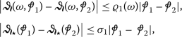(38)

for any $\omega \in \amalg$, ;

($\mathcal{H}_{3}$):

There exist $\varrho _{2}, \varrho _{3} \in C(\amalg , \mathbb{R}_{+})$, $\sigma _{2}, \sigma _{3}>0$ s.t

(39)

for any $\omega \in \amalg$, .

In the following we give a result on the existence and uniqueness of solutions via the generalization of Banach contraction principle.

Theorem 3.2

Assume that ($\mathcal{H}_{2}$) holds. Then the sequential ψ-RL FBVP (10) has a unique solution on ∐, whenever

$$ \frac {\varrho _{1}^{*}}{ \Gamma (\lambda +1)} \bigl( \widehat{\psi}_{ a} ( b ) \bigr)^{\lambda} + 2 \vert \gamma \vert \widehat{\psi}_{ a} ( b) + \sigma _{1}:= \mathring{\kappa} < 1,\quad \Bigl(\varrho _{1}^{*} = \max_{\omega \in \amalg} \bigl\vert \varrho _{1}(\omega ) \bigr\vert \Bigr). $$

(40)

Proof

Clearly, the existence of a solution for ψ-RL FBVP (10) is equivalent to the existence of a fixed point for operator $\mathcal{A}$. For all and $\omega \in \amalg$, using assumption ($\mathcal{H}_{2}$), we have

(41)

Then . Similarly, we obtain

(42)

Hence . Using an induction method, we get , for any $n \in \mathbb{N}$. According to (40), since $\mathring{\kappa}<1$, then we can choose enough large n, s.t $\mathring{\kappa}^{n} <1$. By means of Theorem 2.3, the operator $\mathcal{A}$ has a unique fixed point, giving a unique solution to problem (10). □

Theorem 3.3

Assume that ($\mathcal{H}_{3}$) and the following assertions hold:

• (i) $\frac {\varrho _{2}^{*} ( \widehat{\psi}_{ a} ( b ) )^{\lambda}}{\Gamma (\lambda +1)} + 2|\gamma |\widehat{\psi}_{ a} ( b) + \sigma _{2}:=\mathring{\Xi} < 1$;

• (ii) There exists $M>0$ s.t

  $$ M \biggl[1- \biggl[ \frac { \varrho _{2}^{*} ( \widehat{\psi}_{ a} ( b ) )^{ \lambda}}{ \Gamma (\lambda +1)} + 2 \vert \gamma \vert \widehat{ \psi}_{ a} ( b) + \sigma _{2} \biggr] \biggr] \geq \frac { \varrho _{3}^{*} ( \widehat{\psi}_{ a} ( b ) )^{\lambda}}{ \Gamma (\lambda +1)} + \sigma _{3}, $$

  (43)

where $\varrho _{i}^{*} = \max_{\omega \in \amalg} | \varrho _{i}(\omega )|$, $i=2,3$, then the sequential ψ-RL FBVP (10) has at least one solution on ∐.

Proof

Define the ball $\mathcal{B}_{M} \subset \mathcal{X}_{\mathrm{B}}$ as . Also, define the map $\mathcal{A}: \mathcal{B}_{M} \to \mathcal{X}_{\mathrm{B}}$ as follows:

(44)

Clearly, $\mathcal{B}_{M}$ is a closed convex subset of $\mathcal{X}_{ \mathrm{B}}$. For and $\omega \in \amalg$, we have

(45)

Then, we have , for each . Thus, $\mathcal{A}$ maps $\mathcal{B}_{M}$ into itself. Now, we show that the operator $\mathcal{A}$ is completely continuous. We divide the proof into three steps.

Step 1: Let be a sequence s.t , as $n \to \infty$ in $\mathcal{B}_{M}$. From the continuity of the functions  and Lemma 2.9, for each $\omega \in \amalg$, we have

(46)

which implies that

(47)

Therefore, the operator $\mathcal{A}$ is continuous.

Step 2: From (45), it follows immediately that $\mathcal{A}$ maps bounded sets into bounded sets in $\mathcal{X}_{ \mathrm{B}}$.

Step 3: Next, we will show that $\mathcal{A}(\mathcal{B}_{M})$ is uniformly bounded and equicontinuous. For $a\leq \omega _{1} \leq \omega _{2} \leq b$ and each , using Lemma 2.9, assumption $(\mathcal{H}_{3})$, and the fact that for any and $0\leq p \leq 1$, we have

(48)

Now, we will consider three cases.

Case 1: $a\leq \omega _{1}\leq \omega _{2}\leq \xi \leq b$. In this case, we have

(49)

Case 2: $a\leq \xi \leq \omega _{1}\leq \omega _{2}\leq b$. In this case, we have

(50)

Case 3: $a\leq \omega _{1}\leq \xi \leq \omega _{2}\leq b$. Using a similar argument to that have used to prove the second case, we have

(51)

Thus, $|(\mathcal{A}u)(\omega _{2})-(\mathcal{A}u)(\omega _{1}) | \rightarrow 0$ uniformly as $\omega _{2}\rightarrow \omega _{1}$. Then, $\mathcal{A}$ is a completely continuous operator. Schauder’s fixed point theorem 2.4 guarantees that $\mathcal{A}$ has a fixed point, which is a solution of the sequential ψ-RL fractional boundary value problem (10). □

4 Existence results for system (11)

In this section, we present some existence results for the nonlocal sequential system of fractional differential equations via ψ-RL derivative (11). Let $\mathcal{A} : \mathcal{X}_{\mathrm{B}}^{2} \to \mathcal{X}_{ \mathrm{B}}^{2}$ be the operator defined as $\mathcal{A} = (\mathcal{A}_{1}, \mathcal{A}_{2})$, where $\mathcal{A}_{1}$, $\mathcal{A}_{2}$ are given by

(52)

It is worth noting that a solution of the system (11) can be considered as a fixed point in $\mathcal{X}_{\mathrm{B}}^{2}$ for the completely continuous operator $\mathcal{A}$.

(53)

Firstly, an existence result can be obtained for system (11) by applying Schauder’s fixed-point theorem in $\mathcal{X}_{\mathrm{B}}^{2}$ endowed with vector-valued norm

(54)

For this, we assume the following assumptions

$(\mathcal{H}_{4})$:

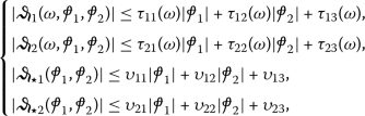(55)

for all $\omega \in \amalg$, , $\tau _{ij} \in C(\amalg , \mathbb{R}_{+})$, $\upsilon _{ij} >0$, $i = \overline{1, 2}$, $j = \overline{1, 3}$.

Theorem 4.1

Assume that ($\mathcal{H}_{4}$) and the following assertion hold:

($\mathcal{H}_{5}$):

The matrix $\mathcal{M}$ defined as

$$ \mathcal{M}:= \begin{pmatrix} \Phi _{11}+ 2 \vert \gamma \vert \widehat{\psi}_{ a} ( b) & \Phi _{12} \\ \Phi _{21} + 2 \vert \gamma \vert \widehat{\psi}_{ a} ( b) & \Phi _{22} \end{pmatrix} , \quad \Phi _{ij} = \frac { \tau _{ij}^{\star}}{ \Gamma ( \lambda + 1)} \bigl( \widehat{\psi}_{ a} ( b ) \bigr)^{\lambda} + \upsilon _{ij}, $$

(56)

converges to zero, where $\tau _{ij}^{\star} = \max_{\omega \in \amalg} \tau _{ij}(\omega )$ and $i = \overline{1,2}$, $j = \overline{1,3}$.

Then system (11) has at least one solution in $\mathcal{X}_{ \mathrm{B}}^{2}$.

Proof

According to the proof of Theorem 3.3, we can easily check that $\mathcal{A}$ is completely continuous. Next, we have to show that $\mathcal{A}$ has a fixed point in a bounded, closed and convex subset of $\mathcal{X}_{\mathrm{B}}^{2}$ of the form

(57)

where

$$ \begin{pmatrix} \mathcal{R}_{1} \\ \mathcal{R}_{2} \end{pmatrix} \geq ( \mathcal{I}- \mathcal{M} )^{-1} \begin{pmatrix} \Phi _{13} \\ \Phi _{23} \end{pmatrix} . $$

(58)

For each and $\omega \in \amalg$, we have that

(59)

Then, we obtain

(60)

Similarly, we get

(61)

If , then Eqs. (60) and (61) can be rewritten as

(62)

or equivalently

(63)

Therefore, from (58), we obtain

(64)

So, we have shown that $\mathcal{A}(\mathcal{B})\subset \mathcal{B}$. Hence, $\mathcal{A}$ has a fixed point by Schauder’s fixed-point Theorem 2.4. □

Next, we use Perov’s fixed-point theorem to prove the existence of unique solution of the sequential system (11). Before we state our result, we list the following assumptions on and , $\dot{ \upiota}=1,2$ for convenience:

$(\mathcal{H}_{5})$:

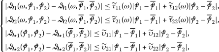(65)

$\forall \omega \in \amalg$, , $\widetilde{\tau}_{ij} \in C(\amalg , \mathbb{R}_{+})$, $\widetilde{\upsilon}_{ij}>0$, $i,j =\overline{1,2}$.

Theorem 4.2

Assume that ($\mathcal{H}_{5}$) and the following assertion hold:

($\mathcal{H}_{6}$):

The matrix $\mathcal{M}$ defined as

$$ \mathcal{M}: = \begin{pmatrix} \Theta _{11}+2 \vert \gamma \vert \widehat{\psi}_{ a} ( b) & \Theta _{12} \\ \Theta _{21} + 2 \vert \gamma \vert \widehat{\psi}_{ a} ( b) & \Theta _{22} \end{pmatrix} , \quad \Theta _{ij} = \frac { \widetilde{\tau}_{ij}^{ \star} }{ \Gamma (\lambda +1)} \bigl[ \widehat{\psi}_{ a} ( b) \bigr]^{\lambda} + \widetilde{\upsilon}_{ij}, $$

(66)

converges to zero, where $\widetilde{ \tau}_{ij}^{\star} = \max_{\omega \in \amalg} \widetilde{\tau}_{ij}(\omega )$, $i,j = \overline{1,2}$. Then system (11) has a unique solution in $\mathcal{X}_{\mathrm{B}}^{2}$.

Proof

We shall prove that $\mathcal{A}$ is a generalized contraction. Let , and $\omega \in \amalg$. Using $(\mathcal{H}_{5})$, we have

(67)

Therefore

(68)

Similarly, one has

(69)

Equations (68)-(69) can be expressed as

(70)

Hence $\|\mathcal{A}(x) - \mathcal{A}( \overline{x}) \| \leq \mathcal{ M } \| x -\overline{x}\|$, where , . This shows that $\mathcal{A}$ is a generalized contraction. Thus, by applying Perov’s fixed-point theorem, the operator $\mathcal{A}$ has a unique fixed point, which is a solution to system (11). □

5 Numerical examples

To validate our theoretical results, we consider the following examples.

Example 5.1

Consider the FBVP

(71)

where $\lambda \in \{ \frac{3}{2}, \frac{8}{5}, \frac{17}{10} \} \subset (1, 2]$, $a=1$, $b=2$, $\eta \in \amalg$, $\gamma = \frac{1}{2}$, $\psi (\omega ) = \sin ( \frac{ \pi}{4} \omega )$, , the nonlinear function , $\xi \geq 0$. By a direct computation, for every and $\omega \in \amalg$, we get

(72)

where $\varrho _{1}(\omega ) = 10 e^{- \xi \omega}$, $\varrho _{1}^{*}= 10 e^{-\xi}$, $\sigma _{1} = \frac{1}{2}$ in conditions ($\mathcal{H}_{2}$). According to Eq. (40), put

(73)

By using the graphical representation of the function ϒ for three cases of λ depicted in Fig. 1, we obtain $\Upsilon (\xi )<0$ for each $\xi \geq \frac{44}{25}, \frac{39}{25}, \frac{34}{25}$, whenever $\lambda =\frac{3}{2}, \frac{8}{5}, \frac{17}{10}$ respectively. Table 1 shows the mentioned values well. Thus, all the conditions of Theorem 3.2 are satisfied, and consequently the sequential ψ-RL FBVP (71) has a unique solution on ∐.

Figure 1

Graph of the function $\Upsilon (\xi )$, for $\lambda \in \{ \frac{3}{2}, \frac{8}{5}, \frac{17}{10} \}$ in Example 5.1

Table 1 $\Upsilon (\xi )$ for $\lambda \in \{ \frac {3}{2}, \frac {8}{5}, \frac {17}{10} \}$ in Example 5.1

The next example shows the correctness of the results based on the changes of function .

Example 5.2

As a second example, in problem (71), consider $\lambda \in \{ \frac{3}{2}, \frac{8}{5}, \frac{17}{10} \}$ and the nonlinear continuous function

(74)

defined on $\amalg \times \mathbb{R}$, $\xi \in [0.3, 5]$, . Hence, for every and $\omega \in \amalg$, we have

where

$$\begin{array}{c}{\varrho }_2(\omega )=5e^{-\xi \omega }⟹{\varrho }_2^{\ast }=5e^{-\xi },\hfill \\ {\varrho }_3(\omega )=ln\sqrt{\xi +\omega }⟹{\varrho }_3^{\ast }=ln\sqrt{\xi +2},\hfill \end{array}$$

(75)

$\sigma _{2} = \frac{1}{4}$, $\sigma _{3} =3$. So, satisfy $(\mathcal{H}_{3})$. Setting

(76)

and by choosing $M=7.8$, we have

(77)

We have 2D plot of the functions $\Xi (\xi )-1$ and $\Pi (\xi )- M$ for three cases of λ in Figs. 2a and 2b respectively. Table 2 shows the mentioned values well. According to the graphical representation, we get $\Xi (\xi ) <1$, and we easily check that

$$ \Xi (\xi ) < 1, \quad \forall \xi \in \textstyle\begin{cases} [0.3, \ 5], & \lambda = \frac{3}{2}, \\ [0.1,\ 5], & \lambda =\frac{8}{5}, \\ [0.1,\ 5], & \lambda =\frac{17}{10}, \end{cases}\displaystyle \qquad \Pi (\xi )< M,\quad \forall \xi \in \textstyle\begin{cases} [2.3, 5], & \lambda = \frac{3}{2}, \\ [2.1, 5], & \lambda =\frac{8}{5}, \\ [1.9, 5], & \lambda =\frac{17}{10}. \end{cases} $$

(78)

Moreover, in Fig. 3, we have 3D plot of $\Pi (\xi ,\lambda )-M$ and $\Xi (\xi ,\lambda )-1$, when $(\xi ,\lambda ) \in [0.3, 5]\times (1,2]$, $[2.3, 5]\times (1,2]$, respectively.

Figure 2

Graph of the functions $\Xi ( \xi )-1$ and $\Pi (\xi )-M$ for $\lambda \in \{ \frac{3}{2}, \frac{8}{5}, \frac{17}{10} \}$ in Example 5.2

Figure 3

3D plots of the functions $\Xi ( \xi ,\lambda )-1$, when $(\xi ,\lambda )\in [0.3,5]\times (1,2]$ and $\Pi (\xi ,\lambda )-M$ for $(\xi ,\lambda )\in [2.3,5]\times (1,2]$ in Example 5.2

Table 2 $\Xi (\xi )-1$ and $\Pi (\xi )-M$, for $\lambda \in \{ \frac {3}{2}, \frac {8}{5}, \frac {17}{10} \}$ in Example 5.2

Therefore, in view of Theorem 3.3, the sequential ψ-RL FBVP (71) has at least one solution on ∐.

In the next example, we check the provided Theorem 4.1 for the sequential ψ-RL nonlinear system with the changes of the ψ function.

Example 5.3

In sequential nonlinear system (11), consider $\lambda \in \{ \frac{3}{2}, \frac{8}{5}, \frac{17}{10} \}$, $\psi (\omega ) = \frac{1}{12}\sqrt{\omega}$, $\gamma = \frac{1}{20}$, $a=1$, $b=2$ and the nonlinear functions

(79)

Obviously, the functions , , $i=\overline{1,2}$ are continuous, and for every and $\omega \in \amalg$, we have

(80)

where

$$\begin{aligned} & \tau _{11}(\omega ) = \frac {1+ \omega}{2+3\omega ^{3}}, \qquad \tau _{12}( \omega ) = e^{-\omega}, \qquad \tau _{13} (\omega ) = \frac {1+\omega}{ 3+2 e^{\omega ^{2}}}, \\ & \tau _{21}(\omega ) = \frac {\omega}{7+\omega ^{2} }, \qquad \tau _{22}( \omega ) = \frac {1}{4(e^{\omega}+3)},\qquad \tau _{23}(\omega ) = e^{-4 \sqrt{\omega}}, \end{aligned}$$

(81)

$\upsilon _{11}=0.5$, $\upsilon _{12} = 10^{-3}$, $\upsilon _{13}= 10^{-1}$, $\upsilon _{21} = 8\times 10^{-2}$, $\upsilon _{22} = 0.1$, $\upsilon _{23}= 10^{-2}$, and

$$ \tau _{11}^{*} = \frac {2}{5},\qquad \tau _{12}^{*} = e^{-1}, \qquad \tau _{21}^{*} = \frac {2}{11}, \qquad \tau _{22}^{*} = \frac {1}{4(3+e)}. $$

From conditions ($\mathcal{H}_{4}$)-($\mathcal{H}_{5}$), a simple computation gives

$$\begin{aligned} \Phi _{ij} & = \frac { \tau _{ij}^{\star}}{ \Gamma ( \lambda + 1)} \bigl( \widehat{ \psi}_{ a} ( b ) \bigr)^{\lambda} + \upsilon _{ij} \\ & \simeq \textstyle\begin{cases} 0.50192, 0.00277, 0.00212, 0.10021, & \lambda = \frac{3}{2}, \\ 0.50128, 0.00217, 0.00183, 0.10014, & \lambda =\frac{8}{5}, \\ 0.50084, 0.00177, 0.00163, 0.10009, & \lambda =\frac{17}{10}, \end{cases}\displaystyle \end{aligned}$$

(82)

and so

$$ \mathcal{M} := \begin{pmatrix} \Phi _{11} + 2 \vert \gamma \vert \widehat{\psi}_{ a} ( b ) & \Phi _{12} \\ \Phi _{21}+2 \vert \gamma \vert \widehat{\psi}_{ a} ( b ) & \Phi _{22} \end{pmatrix} = \textstyle\begin{cases} \begin{pmatrix} 0.50538 & 0.00277 \\ 0.00557 & 0.10021 \end{pmatrix} , & \lambda = \frac{3}{2}, \\ \begin{pmatrix} 0.50473 & 0.00217 \\ 0.00528 & 0.10014 \end{pmatrix} , & \lambda =\frac{8}{5}, \\ \begin{pmatrix} 0.50429 & 0.00177 \\ 0.00508 & 0.10009 \end{pmatrix} ,& \lambda = \frac{17}{10}. \end{cases} $$

(83)

Thus, $\mathcal{M}$ converges to zero for different values of λ. Since all assumptions of Theorem 4.1 are fulfilled, then the sequential nonlinear system (79) has at least one solution in $\mathcal{X}_{\mathrm{B}}^{2}$.

Example 5.4 shows that $\mathcal{M}$ converges to zero for different values of λ.

Example 5.4

According to system (11), we have to consider the following nonlinear functions

(84)

with $\psi (\omega ) = \frac{2 + \omega}{4}$, $\gamma = \frac{1}{400}$, $\xi \geq 1$, and $\lambda \in \{ \frac{3}{2}, \frac{8}{5}, \frac{17}{10} \}$. For any , , , and $\omega \in \amalg$, one has

(85)

where $\widetilde{\tau}_{11}(\omega ) = \frac {1}{ \omega}e^{{\xi}\omega}$, $\widetilde{\tau}_{12}(\omega ) = \frac {1}{14(1+\omega )}$, $\widetilde{\tau}_{11}^{*} = \frac {1}{2}e^{2{\xi}}$, $\widetilde{\tau}_{12}^{*} = \frac {1}{28}$,

$$\begin{aligned}& \widetilde{\tau}_{21}(\omega ) = \frac {1}{20} e^{-\sin ( \frac {\pi \omega}{4} ) },\qquad \widetilde{\tau}_{22}(\omega ) = \frac {1}{3+\xi \cos ( \frac { \omega \pi}{6} )}, \\& \widetilde{\tau}_{21}^{*} = \frac {1}{20}e^{ - \sin ( \frac {\pi }{4} )}, \qquad \widetilde{\tau}_{22}^{*} = \frac {1}{3 + \frac {\xi}{2}}, \end{aligned}$$

(86)

and $\widetilde{\upsilon}_{11} = 0.1$, $\widetilde{\upsilon}_{12} = 0.001$, $\widetilde{\upsilon}_{21} = 0.001$, $\widetilde{\upsilon}_{22} = 0.01$. By a straightforward calculation, we have

(87)

So, we can easily check that

$$ \max \bigl\{ \Theta _{11} + 2 \vert \gamma \vert \widehat{ \psi}_{ a} ( b), \ \Theta _{22} \bigr\} = \Theta _{11} + 2 \vert \gamma \vert \widehat{\psi}_{ a} ( b), \quad \forall \xi \geq 1. $$

(88)

And

$$ \Theta _{11} + 2 \vert \gamma \vert \widehat{ \psi}_{ a} ( b) < 1, \quad \forall \xi \in \textstyle\begin{cases} [1, 1.47526], & \lambda =\frac{3}{2}, \\ [1, 1.58093], & \lambda =\frac{8}{5}, \\ [1, 1.68895], & \lambda =\frac{17}{10}. \end{cases} $$

(89)

Then, $\mathcal{M}$ converges to zero for different values of λ. Thus, all the conditions of Theorem 4.2 are satisfied, and consequently the sequential nonlinear system (84) admits a unique solution $\mathcal{X}_{\mathrm{B}}^{2}$.

6 Conclusion

In this paper, we first establish the Lyapunov-type inequalities of sequential ψ-RL FBVPs, and then using the Banach contraction principle and Schauder’s fixed point, we present two results of the existence and uniqueness of solutions for our problem. Also, two results on the existence of at least one solution, and uniqueness for a sequential nonlinear system of ψ-RL fractional derivative are obtained by applying Schauder’s and Perov’s fixed-point theorems. Examples illustrating the theoretical main results are given.

References

Kilbas, A.A., Srivastava, H.M., J., T.J.: Theory and Applications of Fractional Differential Equations. Elsevier, Amsterdam (2006)
Mainardi, F.: Fractional Calculus and Waves in Linear Viscoelasticity: An Introduction to Mathematical Models. World Scientific, London (2010). https://doi.org/10.1142/p614.
Qu, H., Liu, X.: A numerical method for solving fractional differential equations by using neural network. Adv. Math. Phys. 12 (2015). https://doi.org/10.1155/2015/439526
Zhou, Y.: Basic Theory of Fractional Differential Equations. World Scientific, Singapore (2014)
Podlubny, I.: Fractional Differential Equations. Academic Press, New York (1999)
Mohammadaliee, B., Roomi, V., Samei, M.E.: \(\mathcal{SEIQR}\) model for analyzing COVID-19 with vaccination via conformable fractional derivative and numerical simulation. Sci. Rep. 14, 723 (2024). https://doi.org/10.1038/s41598-024-51415-x
Rezapour, S., Mohammadi, H., Samei, M.E.: SEIR epidemic model for COVID-19 transmission by Caputo derivative of fractional order. Adv. Differ. Equ. 2020, 490 (2020). https://doi.org/10.1186/s13662-020-02952-y
Haddouchi, F.: Positive solutions of nonlocal fractional boundary value problem involving Riemann-Stieltjes integral condition. J. Appl. Math. Comput. 64(1–2), 487–502 (2020). https://doi.org/10.1007/s12190-020-01365-0
Hammad, H.A., Rashwan, R.A., Nafea, A., Samei, M.E., Noeiaghdam, S.: Stability analysis for a tripled system of fractional pantograph differential equations with nonlocal conditions. J. Vib. Control 30(3–4), 632–647 (2024). https://doi.org/10.1177/10775463221149232
Hilfer, R.: Applications of Fractional Calculus in Physics. World Scientific, Singapore (2000). https://doi.org/10.1142/p614
Samko, S.G., Kilbas, A.A., Marichev, O.I.: Fractional Integrals and Derivatives: Theory and Applications. Gordon and Breach Science Publishers, New York (1993)
Samei, M.E., Hedayati, V., Rezapour, S.: Existence results for a fraction hybrid differential inclusion with Caputo–Hadamard type fractional derivative. Adv. Differ. Equ. 2019, 163 (2019). https://doi.org/10.1186/s13662-019-2090-8
Boutiara, A., Benbachir, M., Alzabut, J., Samei, M.E.: Monotone iterative and upper-lower solutions techniques for solving nonlinear ψ-Caputo fractional boundary value problem. Fractal Fract. 5, 194 (2021). https://doi.org/10.3390/fractalfract5040194
Bhairat, S.P., Samei, M.E.: Non-existence of a global solution for Hilfer-Katugampola fractional differential problem. Partial Differ. Equ. Appl. Math. 2023, 100495 (2023). https://doi.org/10.1016/j.padiff.2023.100495
Haddouchi, F.: On the existence and uniqueness of solution for fractional differential equations with nonlocal multi-point boundary conditions. Differ. Equ. Appl. 13(3), 227–242 (2021). https://doi.org/10.7153/dea-2021-13-13
Seemab, A., Rehman, M.U., Alzabut, J., Hamdi, A.: On the existence of positive solutions for generalized fractional boundary value problems. Bound. Value Probl. 2019, 186 (2019). https://doi.org/10.1186/s13661-019-01300-8
Vivek, D., Elsayed, E., Kanagarajan, K.: Theory and analysis of ψ-fractional differential equations with boundary conditions. Commun. Appl. Anal. 22(3), 401–414 (2018). https://doi.org/10.1016/j.aml.2018.08.013
Haddouchi, F.: Existence of positive solutions for a class of conformable fractional differential equations with parameterized integral boundary conditions. Kyungpook Math. J. 61(1), 139–153 (2021). https://doi.org/10.5666/KMJ.2021.61.1.139
Sousa, J.V.C., de Oliveira, E.C.: On the ψ-Hilfer fractional derivative. Commun. Nonlinear Sci. Numer. Simul. 60, 72–91 (2018). https://doi.org/10.1016/j.cnsns.2018.01.005
Katugampola, U.N.: New approach to a generalized fractional integral. Appl. Math. Comput. 218(3), 860–865 (2011). https://doi.org/10.1016/j.amc.2011.03.062
Kiryakova, V.: Generalized Fractional Calculus and Applications. Wiley, New York (1994)
Tarasov, V.: Handbook of Fractional Calculus with Applications: Applications in Physics, Part A. de Gruyter, Berlin (2019)
Promsakon, C., Phuangthong, N., Ntouyas, S.K., Tariboon, J.: Nonlinear sequential Riemann-Liouville and Caputo fractional differential equations with generalized fractional integral conditions. Adv. Differ. Equ. 2018, 385 (2018). https://doi.org/10.1186/s13662-018-1854-x
Ntouyas, S.K., Tariboon, J., Sudsutad, W.: Boundary value problems for Riemann-Liouville fractional differential inclusions with nonlocal Hadamard fractional integral conditions. Mediterr. J. Math. 13, 939–954 (2016). https://doi.org/10.1007/s00009-015-0543-1
Jiang, D., Bai, C.: Existence results for coupled implicit ψ-Riemann-Liouville fractional differential equations with nonlocal conditions. Axioms 11, 3 (2022). https://doi.org/10.3390/axioms11030103
Haddouchi, F., Samei, M.E.: Solvability of a ψ-Riemann-Liouville fractional boundary value problem with nonlocal boundary conditions. Math. Comput. Simul. 219, 355–377 (2024). https://doi.org/10.1016/j.matcom.2023.12.029
Haddouchi, F.: Positive solutions of p-Laplacian fractional differential equations with fractional derivative boundary condition. Sib. Èlektron. Mat. Izv. 18(2), 1596–1614 (2021). https://doi.org/10.33048/semi.2021.18.118
Khalid, K.H., Zada, A., Popa, I.L., Samei, M.E.: Existence and stability of a q-Caputo fractional jerk differential equation having anti-periodic boundary conditions. Bound. Value Probl. 2024, 28 (2024). https://doi.org/10.1186/s13661-024-01834-6
Haddouchi, F.: Existence and Ulam-Hyers stability results for a class of fractional integro-differential equations involving nonlocal fractional integro-differential boundary conditions. Bol. Soc. Parana. Mat. 42 (2024). https://doi.org/10.5269/bspm.64571
Haddouchi, F., Samei, M.E., Rezapour, S.: Study of a sequential ψ-Hilfer fractional integro-differential equations with nonlocal BCs. J. Pseudo-Differ. Oper. Appl. 14, 61 (2023). https://doi.org/10.1007/s11868-023-00555-1
Kumar, D., Yildirim, A., Kaabar, M.K.A., Rezazadeh, H., Samei, M.E.: Exploration of some novel solutions to a coupled Schrödinger-KdV equations in the interactions of capillary-gravity waves. Math. Sci. 18, 291–303 (2024). https://doi.org/10.1007/s40096-022-00501-0
Houas, M., Samei, M.E., Santra, S.S., Alzabut, J.: On Duffing-type oscillator differential equation on the transition to chaos with fractional q-derivatives. J. Inequal. Appl. 12 (2024). https://doi.org/10.1186/s13660-024-03093-6
Almeida, R.: A Caputo fractional derivative of a function with respect to another function. Commun. Nonlinear Sci. Numer. Simul. 44, 460–481 (2017). https://doi.org/10.1016/j.cnsns.2016.09.006
Kuche, K.D., Mali, A.D.: On the nonlinear \((k, \psi )\)-Hilfer fractional differential equations. Chaos Solitons Fractals 152, 14 (2021). https://doi.org/10.1016/j.chaos.2021.111335
Ntouyas, S.K., Bashir, A., Nuchpong, C., Tariboon, J.: On \((k,\psi )\)-Hilfer fractional differential equations and inclusions with mixed \((k,\psi )\)-derivative and integral boundary conditions. Axioms 11(8), 403 (2022). https://doi.org/10.3390/axioms11080403
Almeida, R., Malinowska, A.B., T., M.M.T.: Fractional differential equations with a Caputo derivative with respect to a kernel function and their applications. Math. Methods Appl. Sci. 41(1), 336–352 (2018). https://doi.org/10.1002/mma.4617
Siddiqi, A.H.: Functional Analysis with Applications. Tata McGraw-Hill Publishing ltd, New Delhi (1986)
Smart, D.R.: Fixed Point Theorems. Cambridge University Press, Cambridge (1980)
Precup, R.: Methods in Nonlinear Integral Equations. Kluwer, Dordrecht-Boston-London (2002)
Precup, R.: The role of matrices that are convergent to zero in the study of semilinear operator systems. Math. Comput. Model. 49(3–4), 703–708 (2009). https://doi.org/10.1016/j.mcm.2008.04.006
Agarwal, R.P., Meehan, M., O’Regan, D.: Fixed Point Theory and Applications. Cambridge University Press, Cambridge (2001)
Acknowledgements
Not applicable.
Funding
Author information
Authors and Affiliations
Contributions
All authors are equally contributed, read and approved the final manuscript.
Corresponding author
Ethics declarations
Ethics approval and consent to participate
Consent for publication
Competing interests
The authors declare no competing interests.
Additional information
Publisher’s Note
Springer Nature remains neutral with regard to jurisdictional claims in published maps and institutional affiliations.
Rights and permissions
Open Access This article is licensed under a Creative Commons Attribution 4.0 International License, which permits use, sharing, adaptation, distribution and reproduction in any medium or format, as long as you give appropriate credit to the original author(s) and the source, provide a link to the Creative Commons licence, and indicate if changes were made. The images or other third party material in this article are included in the article’s Creative Commons licence, unless indicated otherwise in a credit line to the material. If material is not included in the article’s Creative Commons licence and your intended use is not permitted by statutory regulation or exceeds the permitted use, you will need to obtain permission directly from the copyright holder. To view a copy of this licence, visit http://creativecommons.org/licenses/by/4.0/.
About this article
Cite this article
Haddouchi, F., Samei, M.E. On the existence of solutions for nonlocal sequential boundary fractional differential equations via ψ-Riemann–Liouville derivative. Bound Value Probl 2024, 78 (2024). https://doi.org/10.1186/s13661-024-01890-y
Received:
Accepted:
Published:
DOI: https://doi.org/10.1186/s13661-024-01890-y