
Abstract
The main objective of this paper is to investigate the dynamic bifurcation for the granulation convection in the solar photosphere. Based on the dynamic bifurcation theory, which is established by Ma and Wang (Phase transition dynamics, pp. 380-459, 2014), the critical parameters \((R,F)\) condition for the granulation convection is derived. Furthermore, the corresponding R-F-phase diagram is generated. In addition, the bifurcation solution is also obtained with certain assumptions.
1 Introduction
The atmosphere of the sun is divided into three parts: the bottom layer of the atmosphere is photosphere, the middle layer is chromosphere and the outermost layer is the corona. The grainy appearance of solar photosphere is produced by the tops of the convective cells and is called granulation. It worth noting that Kutner analyzed the structure of granulation in his book [2]. He pointed out that the temperature decreases with the increasing height in the photosphere. And he concluded that the temperature difference between the top and bottom of photosphere causes the granulation convection in photosphere which can be explained by circulation cells of material. In circulation cells, the hotter gas is brought up from below, producing the bright regions. The cooler gas, which produces the darker regions, is carried down to replace the gas that was brought up (see Figure 1).

The structure of granulation. This is a lateral view showing the situation under the surface. The hotter gas is brought up from below, producing the bright regions. The cooler gas, which produces the darker regions, is carried down to replace the gas that was brought up.
In addition, Ustyugov introduced the solar activity and gave the magneto-hydrodynamics (MHD) equations in [3, 4], which can explain the convection structure in the sun. There have been many studies on this kind of problem. For instance, Chae [5], Agélas [6], and Wu [7] considered the regularity of MHD equations, and Capone [8] and Fuchs [9] studied the stability bifurcation of MHD equations. For more research about the MHD equations refer to [10–17]. It is noticed that the granulation convection structure (see Figure 1) is similar to the structure of Rayleigh-Bénard convection and the Taylor problem. Inspired by the dynamic theory, which is established by Ma and Wang to study the Rayleigh-Bénard convection and the Taylor problem (see [1, 18–20]), we will investigate the dynamic bifurcation for the granulation convection. This paper is organized as follows.
-
1.
In Section 2, we introduce the equations governing the atmospheric circulation with magnetic field and also give the bifurcation theory.
-
2.
Section 3 is devoted to getting the RF-phase diagram of granulation under the parametric condition \(K_{1}=0\) and \(F\neq0\), where R is the Rayleigh number, which is related to the difference of temperature \(T_{1}-T_{0}\), F is a dimensionless parameter, which is related to the magnetic field H, and \(K_{1}\) is as in (2.5), which is related to the boundary condition \(H_{0}\) and \(H_{1}\). The transition occurs as the parameter \((R, F)\) crosses the critical curve L from region I to region II; see Figure 2.
Figure 2 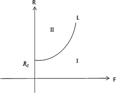
The RF-phase diagram. In region I, there is no granulation convection structure; and in region II, the granulation appears. So the transition occurs as the parameter (R,F) crosses the critical curve L from region I to region II.
-
3.
In Section 4, the bifurcation solution and the critical Rayleigh number \(R_{C}\) are obtained under the condition \(F= 0\).

2 Governing equations
2.1 The model in spherical coordinates
Let \((\varphi, \theta,r)\) be the spherical coordinates, where φ, θ, r represent the longitude, the latitude, and the radial coordinate, respectively. The unknown functions include the velocity field \(u=(u_{\varphi},u_{\theta},u_{r})\), the temperature function T, the pressure function p, the electromagnetic press function Φ and the magnetic field \(H=(H_{\varphi},H_{\theta},H_{r})\). Then the equations governing the atmospheric circulation with magnetic field [9, 21–23] in the spherical coordinates are given by
where \(0\leq\varphi\leq2\pi\), \(-\frac{\pi}{2}\leq\theta\leq\frac{\pi }{2}\), \(r_{0}< r< r_{1}\), \(r_{1}=r_{0}+d\), \(r_{0}\) is the radius of the sun, and d is the height of the troposphere, \(\vec{k}=(0,0,1)\), g is the gravitative constant, ν is the kinetic viscosity, κ is the thermal diffusivity, and η is the resistivity. The differential operators in the spherical coordinates are given as follows:
△̄H, ∇Φ, divH are similar to △̄u, ∇p, divu, and the operators Δ, \((u\cdot\nabla)\) are given by
In this paper, we mainly focus on the dynamic bifurcation for the granulation. For simplicity, we assume \(\theta=\frac{\pi}{2}\). Then the velocity component \(u_{\theta}\) and the magnetic field \(H_{\theta}\) are zero, and equations (2.1) become
where
Furthermore, equations (2.2) are supplemented with the following boundary condition:
2.2 Perturbed dimensionless equations
We determine the basic flow by following assumptions.
-
1.
\(U=(u_{\varphi},u_{r},T,H_{\varphi} ,H_{r})=(0,0,\tilde {T}(r),0,\tilde{H}_{r})\), \(p=\tilde{p}(r)\), \(\Phi=0\); that is, the pressure function, the temperature function and the magnetic field function in r-direction are not zero, and which are only depending on r.
-
2.
The functions \(\tilde{T}(r)\), \(\tilde{H}(r)\) and \(\tilde{p}(r)\) satisfy
$$ \left\{ \textstyle\begin{array}{l} -\frac{1}{\rho_{0}}\frac{\partial\tilde{p}}{\partial r}-g [1-\alpha (\tilde{T}-T_{0}) ]=0, \\ \triangle\tilde{T}=0, \\ \triangle\tilde{H_{r}}-\frac{2}{r^{2}}\tilde{H_{r}}=0. \end{array}\displaystyle \right . $$ -
3.
Based on the boundary condition (2.3), the value of basic flow on the boundary is given by
$$ \begin{gathered} \tilde{H_{r}}=H_{0},\qquad \tilde{T }=T_{0},\qquad r=r_{0}, \\ \tilde{H_{r}}=H_{1},\qquad \tilde{T }=T_{1},\qquad r=r_{0}+d. \end{gathered} $$
From the above assumptions, we derive the basic flow as follows:
where
It is noticed that \(K_{0}\) and \(K_{1}\) are related to the boundary value \(H_{0}\) and \(H_{1}\). Furthermore, in order to get the perturbation equations related to the variables r and φ, we make the following translations:
Omitting the primes, equations (2.2) can be rewritten as
As we know, the radius of the sun is about \(7\times10^{5}\mbox{ km}\) and the thickness of the photosphere is about 500 km. Then the ratio of the thickness of the photosphere to the radius of the sun is small. Hence, we adopt the approximations that \(1/r \simeq1/r_{0}\), \((r_{0}+d)/r_{0}\simeq1 \). For simplicity, we assume \(\nu/\kappa=\eta/\kappa=1\). Also, we introduce the following dimensionless variables:
where R, called the Rayleigh number, is a dimensionless parameter and
Let \((\varphi'', r'')=(r_{0}\varphi', r')\). With the above assumptions, we omit the primes and get the approximate equations, which are given as follows:
where \((\varphi,r)\in M=(0,L)\times(r_{0},r_{0}+1)\), \(r_{0}\) is the radius of the sun with the unit of d, \(L=2\pi r_{0}\), and \(K_{0}\), \(K_{1}\) are given as (2.5). \((u\cdot\nabla)\), div and △ are general differential operators.
The boundary conditions (2.3) are rewritten as
2.3 Abstract operator equation
Now we will show that equations (2.7) can be written in the operator form. Since the velocity field u and the magnetic field H on M are divergence-free, there exist the following stream functions \(f_{1}\) and \(f_{2}\) satisfying the given boundary condition:
Moreover, the following two vector fields:
are gradient fields, which can be balanced by ∇p and ∇Φ in (2.7). Hence, (2.7) are equivalent to the following equations:
To get the abstract form of (2.9), we define the following spaces:
Now, we define the operators \(L=-A+B: H_{1}\rightarrow H\) and \(G: H_{1}\rightarrow H\) by
where \(P: L^{2}(M, R^{5})\rightarrow H\) is the Leray projection, \(U=(u,T,H)\in H_{1}\) and
Therefore, the problem (2.9) with boundary conditions (2.8) are equivalent to the following abstract equation.
where \(\lambda=(R,F)\in R^{2}\) is the parameter and \(U_{0}\) is the initial value of (2.9).
3 Under the condition \(K_{1}=0\)
In this section, we study (2.9) the case that \(K_{1}=0\). Hence, the boundary condition in (2.5) satisfies
We choose the Rayleigh number and the F-number as the control parameters, which are given as follows:
Then we consider the following eigenvalue equations of (2.9):
with the boundary conditions (2.8). We proceed with the separation of variables. Under the periodic boundary condition (2.8), the problem (3.2) possesses two eigenvectors: Ψ and Ψ̃ in the following forms:
where \(a_{k}= 2k\pi/L\). Putting \((\Psi,p,\Phi)\) and \((\tilde{\Psi},\tilde{p},\tilde{\Phi})\) into (3.2), respectively, we deduce from (3.2), (3.3) and (3.4) that \((h_{k},g_{k},T_{k},p_{k},\Phi_{k})\) satisfy the eigenvalue problems,
for any \(k\in Z\), with \(k\neq0\), where
We infer from (3.5) and the boundary conditions (2.8) that the \(h_{k}\) satisfy the equations
By (3.7), the \(h_{k}\) are sine functions, i.e.,
Putting (3.8) into (3.6), we see that
where
It is well known that all solutions of the cubic equation (3.9) \(\beta_{kl}\) are eigenvalues of (3.2). Let \(\beta_{kl}^{i}\) (\(1\leq i\leq3\)) be three zero points of (3.9). It is easy to see that \(Re\beta_{kl}^{1}\geq Re\beta _{kl}^{2}\geq Re\beta_{kl}^{3}\). Furthermore, \(\beta=0\) is a zero point of (3.9) if and only if
where
where \(\alpha_{kl}\) and \(a_{k}\) are as defined in (3.10). When \(F=0\), we can get the critical Rayleigh number \(R_{C}\)
Then the critical parameter curve in Figure 2 is given by
where \(b_{k_{0}l_{0}}\), \(c_{k_{0}l_{0}}\) and \(d_{k_{0}l_{0}}\) as in (3.11) and (3.12).
Lemma 3.1
Let \((k,l)=(k_{0},l_{0})\) minimize the right hand side of (3.12) and the zero point \(\beta_{k_{0}l_{0}}^{1}\) of (3.9) is a real single eigenvalue of (3.2) near curve L. Then \(\beta _{k_{0}l_{0}}^{1}\) satisfies
\(\beta_{kl}^{i}<0\), \(\forall(k,l,i)\neq(k_{0},l_{0},1)\), and \((R,F)\) near L, where the region I and II are as Figure 2.
Proof
We first prove that
In fact, as \((R,F)=(0,0)\), the solutions of (3.9) are
Namely, \(\beta_{k_{0}l_{0}}^{1}(0,0)<0\). Since \(\beta_{k_{0}l_{0}}^{1}(R,F)\) are continuous on \((R,F)\), then (3.14) holds true. Next, we are ready to prove that the first eigenvalue \(\beta _{k_{0}l_{0}}^{1}(R,F)>0\) in region II near the curve L. Let
where \(L_{k_{0}l_{0}}=b_{k_{0}l_{0}}-c_{k_{0}l_{0}}R+d_{k_{0}l_{0}}F^{2}\). When \(L_{k_{0}l_{0}}= 0 \), \(\Gamma_{1}\) is the graph of \(g_{k_{0}l_{0}}\); when \(L_{k_{0}l_{0}}< 0\), \(\Gamma_{2}\) is the graph of \(g_{k_{0}l_{0}}\), as shown in Figure 3. Then the intersecting point of \(\Gamma_{i}\) (\(i=1,2\)) and β-axis is the first eigenvalue \(\beta_{k_{0}l_{0}}^{1}\). When \(L_{k_{0}l_{0}}=0\), the intersecting point of \(\Gamma_{1}\) and β-axis, \(\beta _{k_{0}l_{0}}^{1}= 0\), and \((R,F)\) is in curve L. When \(L_{k_{0}l_{0}}< 0\), the intersecting point of \(\Gamma_{2}\) and β-axis, \(\beta _{k_{0}l_{0}}^{1}> 0\), and \((R,F)\) is in region II. At last, we will show that \(\beta_{kl}^{i}<0\), \(\forall(k,l)\neq(k_{0},l_{0})\), when \((R,F)\) in region I or in region II near the curve L. We only need
Otherwise, if (3.15) does not hold true, there exist a pair of \((R_{1},F_{1})\), such that \(\beta_{kl}^{i}(R_{1},F_{1})=0\). That is to say, there exists a curl \(L_{kl}\), which passes through the point \((R_{1},F_{1})\) and intersects with R-axis at \(R_{C_{1}}\), as shown in Figure 4. It is easy to find that \(R_{C}> R_{C_{1}}\), which makes a contradiction that \(R_{C}\) is the minimum critical Rayleigh number. So, we prove (3.15). When \((R,F)=(0,0)\), we have
which implies \(\beta_{kl}^{i}<0\), \(\forall(k,l)\neq(k_{0},l_{0})\). Because \(\beta_{kl}^{i}(R,F)\) are continuous, \(\beta_{kl}^{i}<0\) in region I or in region II near the curve L. This proves Lemma 3.1.

The graph of \(\pmb{g_{k_{0}l_{0}}}\) . As the figure shows: When \(L_{k_{0}l_{0}}= 0 \), \(\Gamma_{1}\) is the graph of \(g_{k_{0}l_{0}}\); when \({L_{k_{0}l_{0}}< 0}\), \(\Gamma_{2}\) is the graph of \(g_{k_{0}l_{0}}\),Then the intersecting point of \(\Gamma_{i}\) (\(i=1,2\)) and β-axis is the first eigenvalue \(\beta_{k_{0}l_{0}}^{1}\). When \(L_{k_{0}l_{0}}=0\), the intersecting point of \(\Gamma_{1}\) and β-axis, \(\beta _{k_{0}l_{0}}^{1}= 0\), and \({(R,F)}\) is in curve L. When \(L_{k_{0}l_{0}}< 0\), the intersecting point of \(\Gamma_{2}\) and β-axis, \(\beta _{k_{0}l_{0}}^{1}> 0\), and \((R,F)\) is in region II.

The graph of \(\pmb{L_{kl}}\) . The curl \(L_{kl}\) passes through the point \((R_{1},F_{1})\) and intersects with the R-axis at \(R_{C_{1}}\), it is easy to find that \(R_{C}> R_{C_{1}}\).
□
Based on Theorem 2.3.1 in [1], Theorem 2 in [20] and Lemma 3.1, we derive the following theorem.
Theorem 3.2
The critical parameter curve L divides the RF-plane into two regions I and II (see Figure 2), such that the following conclusions hold true.
-
1.
If \((R,F)\in\textit{I}\), the problem (2.8) and (2.9) have no bifurcation, and the basic flow in (2.4) with \(K_{1}=0\) is stable.
-
2.
If \((R,F)\in\textit{II}\), there exists a bifurcation solution.
-
3.
The transition takes place as the control parameter \((R,F)\) crosses the critical curve L from region I into II.
4 For the condition that \(K_{1}\neq0\) and \(F=0\)
4.1 Eigenvalue problem
Consider the case that \(F=0\), and F is given by (2.10). Then equations (2.9) become
Essentially, the control parameter in (4.1) is only the Rayleigh number R in (3.1). Then the eigenvalues and the eigenvectors Ψ, Ψ̃ are similar to those in Section 3, and we can get the corresponding eigenvalue problems
From (4.2), we see that \(g_{k}\) (\(k=1,2,\ldots \)) satisfy the equations
By (4.2) and the boundary conditions (2.8), \(g_{k}\) are the sine functions
Moreover, \(h_{k}\) and \(T_{k}\) are determined by the following:
Substituting \(g_{kl}\) into (4.3), we see that the eigenvalue β of (4.2) satisfies the cubic equation
Hence, all eigenvalues and eigenvectors can be derived from the following cases.
-
1.
For \((k,l)=(0,l)\), we have
$$\begin{gathered} \beta_{0l}^{1}=-l^{2}\pi^{2},\qquad \beta_{0l}^{2}=-l^{2}\pi^{2}- \frac {1}{r_{0}^{2}}, \\\Psi_{0l}^{1}= \bigl(0,0,\sin l\pi(r-r_{0}),0,0 \bigr),\qquad\tilde{\Psi} _{0l}^{1}= \bigl(0,0,\cos l \pi(r-r_{0}),0,0 \bigr), \\\Psi_{0l}^{2}= \bigl(0,0,0,\cos l\pi(r-r_{0}),0 \bigr),\qquad\tilde{\Psi }_{0l}^{2}= \bigl(0,0,0,\sin l \pi(r-r_{0}),0 \bigr). \end{gathered}$$ -
2.
For \((k,l)=(k,0)\), the eigenvalues and eigenvectors are given by
$$\begin{gathered} \beta_{k0}=-a_{k}^{2}-\frac{2}{r_{0}^{2}}, \\\Psi_{k0}=(0,0,0,0,\sin a_{k}\varphi),\qquad\tilde{\Psi }_{k0}=(0,0,0,0,\cos a_{k}\varphi). \end{gathered}$$ -
3.
For \(k\neq0\) and \(l\neq0\), it is well known that all solutions of equation (4.6) are eigenvalues. Let \(\beta_{kl}^{1}(R)\) (\(1\leq i\leq3\)) be three zero points of (4.6) such that
$$Re\beta_{kl}^{1}\geq Re\beta_{kl}^{2} \geq Re\beta_{kl}^{3}. $$
Then, by (3.3), (3.4), (4.4) and (4.5), the eigenvectors \(\Psi_{kl}^{i}\) and \(\tilde{\Psi}_{kl}^{i}\) corresponding to \(\beta_{kl}^{1}\) can be written as
where
It is clear that the eigenvalues and eigenvectors have the following properties.
-
1.
\(\beta_{0l}^{i}\), \(\beta_{k0}\) and \(\beta_{kl}^{i}\) (\(k\neq0\), \(l\neq 0\)) consist of all eigenvalues of equation (4.2), and all eigenvectors form a basis of H;
-
2.
\(\beta_{0l}^{i}< 0\) (\(i=1,2\)) and \(\beta_{k0}< 0\);
-
3.
the eigenvalues \(\beta_{kl}^{i}\) (\(k\neq0\), \(l\neq0\)) only depend on the Rayleigh number.
Now, we are ready to determine the dual eigenvector. The dual eigenvectors \(\Psi_{kl}^{i\ast}\) and \(\tilde{\Psi}_{kl}^{i\ast}\) are given by
where
Thus, all dual eigenvectors consist of \(\Psi_{0l}^{1\ast}=(0,0,\sin l\pi (r-r_{0}),0,0)\), \(\Psi_{0l}^{2\ast}=(0,0,0, \sin l\pi(r-r_{0}),0)\), \(\Psi_{k0}^{\ast}=(0,0,0,0,\sin a_{k}\varphi)\), \(\tilde{\Psi}_{k0}^{\ast }=(0,0,0,0,\cos a_{{k}}\varphi)\).
In this part, we are ready to study the critical-crossing of the first eigenvalue. Since the eigenvalues \(\beta_{kl}^{i}\) (\(1\leq i\leq3\), \(k\neq0\), \(l\neq0\)) only depend on the Rayleigh number, it suffices to focus on the eigenvalue problem (4.6). If \(\beta=0\) is a zero point of (4.6), we can get
In this case, we have
Hence the critical Rayleigh number \(R_{C}\) has a similar form to Section 3, which is given by
Thus, we have the following lemma.
Lemma 4.1
Let \((k_{0},l_{0})\) minimize the right hand side of (4.11). Assume the zero point \(\beta_{k_{0}l_{0}}^{1}\) of (4.6) is a real single eigenvalue of (4.1) near \(R_{C}\), then \(\beta_{k_{0}l_{0}}^{1}\) satisfies
The proof is similar to the proof of Lemma 3.1, so we omit it.
4.2 Transition theory with \(F=0\)
In this section, we consider the transition theorem of problem (4.1) with boundary conditions (2.8) with \(K_{1}\neq0\) and \(F=0\), where \(K_{1}\), F as in (2.10). Then we have the following theorem.
Theorem 4.2
Let \(K_{1}\neq0\) and \(F=0\), we have the following conclusions for equations (4.1) with boundary conditions (2.8).
-
1.
Equation (4.1) bifurcates from \(((u,T,H),R)=(0,R_{C})\) to an attractor \(\Sigma_{R}\in H_{1}\), only consisting of a steady state solution.
-
2.
The steady state solution \((u,T,H)=(u_{\varphi},u_{r},T,H_{\varphi },H_{r})\) can be expressed as
$$(u_{\varphi},u_{r},T,H_{\varphi},H_{r})=C \bigl( \beta _{k_{0}l_{0}}^{1}(R) \bigr)^{\frac{1}{2}} \bigl(x \Psi_{k_{0}l_{0}}^{1} +y\tilde{\Psi}_{k_{0}l_{0}}^{1} \bigr)+o \bigl(\big|\beta_{k_{0}l_{0}}^{1}\big|^{\frac{1}{2}} \bigr), $$where \(C>0\) is a constant, \(\Psi_{k_{0}l_{0}}^{1}\) and \(\tilde{\Psi }_{k_{0}l_{0}}^{1}\) are the first eigenvectors given by (4.7) and (4.8), and \(x^{2}+y^{2}=1\).
Proof
We first reduce the abstract equation (2.11) to the center manifold. Let \(J_{0}=(k_{0},l_{0},1)\), then \(\Psi_{k_{0}l_{0}}^{1}=\Psi_{J_{0}}\) and \(\tilde{\Psi }_{k_{0}l_{0}}^{1}= \tilde{\Psi}_{J_{0}}\), the reduced equations read
where \(U=(u_{\varphi},u_{r},T,H_{\varphi},H_{r})\in H_{1}\) is written as
Φ is the center manifold function, and G is a bilinear operator, which is
It is easy to verify that
Hence, (4.12) can be rewritten as
Based on the approximation formula Theorem 6.1 in[18] for center manifold functions, we see that the manifold function Φ satisfies
By direct calculation, from (4.15), the center manifold function can be written
Inserting (4.16) into (4.14), we have
where
Therefore, the conclusions of Theorem 4.2 follows from (4.17), (4.18) and the attractor bifurcation theorem in [3]. The proof of the theorem is completed. □
5 Conclusions
In summary, the production of granulation convection is illustrated by Theorem 3.2 and Figure 2, where \(R_{C}\) is the critical Rayleigh number. As is shown in Figure 2, when the differences of temperature and magnetic are small enough, the points \((R,F)\) are below the critical curve L and in region I, the gas is in a static state. When they become greater than the curve L, the gas suddenly breaks into regular circulation cells, which is granulation convection. The circulation cells can be expressed by the bifurcation solution in Theorem 4.2. From both the mathematical and the physical points of view, the results are valuable to understand the phase transition in fluid dynamics.
References
Ma, T, Wang, S: Phase Transition Dynamics, pp. 380-459. Springer, New York (2014)
Kutner, ML: Astronomy: A Physical Perspective, pp. 101-108. Cambridge University Press, Cambridge (2003)
Ustyugov, SD: Hyperbolic Problems: Theory, Numerics, Applications, pp. 1061-1068. Springer, Berlin (2008)
Ustyugov, DO, Ustyugov, SD: Simulation of radiation expansion of laser plasma in an external magnetic field. Math. Models Comput. Simul. 2(3), 362-374 (2010)
Chae, D, Wolf, J: On partial regularity for the steady Hall magnetohydrodynamics system. Commun. Math. Phys. 339(3), 1147-1166 (2015)
Agélas, L: Global regularity for logarithmically critical 2D MHD equations with zero viscosity. Monatshefte Math. 181(2), 245-266 (2016)
Wu, JH: Global regularity for a class of generalized magnetohydrodynamic equations. J. Math. Fluid Mech. 13(2), 295-305 (2011)
Capone, F, Rionero, S: Porous MHD convection: stabilizing effect of magnetic field and bifurcation analysis. Ric. Mat. 65(1), 163-186 (2016)
Fuchs, H, Rädler, K: Bifurcations in spherical MHD models. Stud. Geophys. Geod. 42(3), 320-327 (1998)
Gala, S: A note on the blow-up criterion of smooth solutions to the 3D incompressible MHD equations. Acta Math. Sin. 28(4), 639-642 (2012)
Yong, Y, Jiu, QS: Energy equality and uniqueness of weak solutions to MHD equations in \(L{\infty}(0,T;L_{n}(\Omega))\). Acta Math. Sin. 25(5), 803-814 (2009)
Su, M, Wang, J: Global smooth solutions to 3D MHD with mixed partial dissipation and magnetic diffusion. J. Inequal. Appl. 2013, Article ID 345 (2013)
Ellahi, R: The effects of MHD and temperature dependent viscosity on the flow of non-Newtonian nanofluid in a pipe: analytical solutions. Appl. Math. Model. 37(3), 1451-1467 (2013)
Ellahi, R, Zeeshan, A, Hassan, M: Particle shape effects on Marangoni convection boundary layer flow of a nanofluid. Int. J. Numer. Methods Heat Fluid Flow 26(7), 2160-2174 (2016)
Marin, M, Marinescu, C: Thermoelasticity of initially stressed bodies, asymptotic equipartition of energies. Int. J. Eng. Sci. 36(1), 73-86 (1998)
Marin, M, Lupu, M: On harmonic vibrations in thermoelasticity of micropolar bodies. J. Vib. Control 4(5), 507-518 (1998)
Marin, M: A domain of influence theorem for microstretch elastic materials. Nonlinear Anal., Real World Appl. 11(5), 3446-3452 (2010)
Ma, T, Wang, S: Stability and Bifurcation of Nonlinear Evolution Equation, pp. 242-264. Science Press, Beijing (2007)
Ma, T, Wang, S: Rayleigh-Bénard convection: dynamics and structure in the physical space. Commun. Math. Sci. 5(3), 553-574 (2007)
Ma, T, Wang, S: Stability and bifurcation of the Taylor problem. Arch. Ration. Mech. Anal. 181(1), 146-176 (2006)
Günther, U, Stefani, F: Isospectrality of spherical MHD dynamo operators. J. Math. Phys. 44(7), 3097-3111 (2002)
Sekhar, TVS, Sivakumar, R, Kumar, TVRR, Vimala, S: Numerical simulations of highly non-linear coupled full MHD equations in spherical geometry. Int. J. Non-Linear Mech. 47(6), 599-615 (2012)
Rohde, C, Zajaczkowski, W: On the Cauchy problem for the equations of ideal compressible MHD fluids with radiation. Appl. Math. 48(4), 257-277 (2003)
Acknowledgements
The author would like to thank the referee for invaluable comments insightful suggestions. This article was supported by the National Natural Science Foundation of China (A0109).
Author information
Authors and Affiliations
Corresponding author
Additional information
Competing interests
The author declares to have no competing interests.
Author’s contributions
The author discussed, read and approved the final version of the manuscript.
Publisher’s Note
Springer Nature remains neutral with regard to jurisdictional claims in published maps and institutional affiliations.
Rights and permissions
Open Access This article is distributed under the terms of the Creative Commons Attribution 4.0 International License (http://creativecommons.org/licenses/by/4.0/), which permits unrestricted use, distribution, and reproduction in any medium, provided you give appropriate credit to the original author(s) and the source, provide a link to the Creative Commons license, and indicate if changes were made.
About this article

Cite this article
Li, J. Dynamic bifurcation for the granulation convection in the solar photosphere. Bound Value Probl 2017, 110 (2017). https://doi.org/10.1186/s13661-017-0842-5
Received:
Accepted:
Published:
DOI: https://doi.org/10.1186/s13661-017-0842-5