
Abstract
We study a “conjugate” transform on matrix spaces. For Laurent/Toeplitz operators such a transform is a way of realizing the Hilbert transform on the torus. We establish its operator norm on Schatten classes and discuss the possibility of its boundedness upon permutations. Applications in the Rademacher–Menshov inequality and iterative methods are also included.
1 Motivation
We consider the following transform T̃ on matrix spaces:
where ∘ is the Hadamard product, , and
If \(H=L+L^{*}\) (∗ denotes the adjoint) with L being strictly lower triangular, then
thus T̃ simply takes the “real” part of L to its “imaginary” part, because of this it should be reasonable to call T̃ the conjugate transform.
Another good reason for such a name is the connection of T̃ to the Hilbert transform on the torus, which is defined as
(p.v. stands for Cauchy principal value). The Fourier series of f and f̃ differ by a sign depending on the frequency term, i.e., if , then [1, Chap. 6].
Take , it induces a bounded multiplication operator on by \(g\mapsto fg\). We can expand f into Fourier series (recall that , and by the Carleson theorem the series also converges a.e. [2, 3]) and write it as a vector \((\ldots , \hat{f}(-1), \hat{f}(0), \hat{f}(1),\ldots )^{T}\). In this way the multiplication operator induced by f can be represented by a bi-infinite Toeplitz matrix F (i.e., a Laurent operator) with \(F_{ij}=\hat{f}(k)\) if \(j-i=k\) (alternatively see [4, Chap. 1] or [5, Chap. 3]). It then follows that the multiplication operator \(g\mapsto \tilde{f}g\) can be represented by the matrix \(\tilde{T}(F)\), thus T̃ on matrix forms of Laurent/Toeplitz operators is a way of realizing the Hilbert transform on (see also [6] for a different perspective where T̃ is viewed as the bilinear Hilbert transform on Hankel operators).
Moreover, we have
The right-hand side is called the Riesz projection of f, on Toeplitz matrices it corresponds to
where D̃ is the diagonal projection that maps A to its main diagonal, and L̃ is the triangular truncation that maps A to its strict lower triangular part. Since D̃ is for many norms bounded, the boundedness of L̃ can then essentially be determined by inspecting T̃.
The truncation L̃ appears at various places in mathematics, for example, in numerical analysis, L̃ enters critically into the iteration matrix for the Gauss–Seidel method and the Kaczmarz method, the error reduction rate with respect to the spectral condition number can be estimated using the spectral operator norm of L̃ (see [7, 8]); In functional analysis, L̃ on finite dimensional spaces is the explicit form of the projection that maps a Schatten class to the subclass of Volterra operators in it (see [9, Chap. 3] or [10]); In harmonic analysis, the norm of majorant function in the Rademacher–Menshov inequality [11, 12] can be estimated by the norm L̃ (see [13]). Therefore, as simple as the form of T̃ (and L̃) is, its rich and profound background intrigues us to understand its behavior on .
To our interest is the Schatten class \(S_{p}\), which consists of compact operators whose singular values are in \(\ell ^{p}\). \(S_{p}\) is a Banach space equipped with the \(\ell ^{p}\) norm of its singular values. \(S_{1}\), \(S_{2}\), \(S_{\infty}\) norms are nuclear, Hilbert–Schmidt, and spectral norms respectively. We use \(\|\cdot \|_{p}\) to denote the \(S_{p}\) norm of a matrix, if \(p=\infty \), then the subscript is omitted.
For integral operators, it is known that if their symbol belongs to particular mixed norm spaces \(L^{p,q}\) (p, q are Hölder conjugates with \(p\ge 2\)), then they are in the Schatten class \(S_{p}\) (see [14–16]). On the other hand, the Hilbert transform is bounded on for \(1< p<\infty \) (known as the Marcel–Riesz inequality [1, Chap. 6.17]) and unbounded on (thus also unbounded on by duality and its anti-symmetry [17, Theorem 102]), an explicit example of this unboundedness can be found in [18, p. 250].
Such insights suggest that T̃ acts on \(S_{p}\) the same way as the Hilbert transform behaves on \(L^{p}\), which brings us to the main result of this paper:
Theorem 1
-
(i)
The operator norm \(\|\tilde{T}\|_{\infty}\) of T̃ on with respect to the \(S_{\infty}\) norm is
$$ \Vert \tilde{T} \Vert _{\infty}=\frac{1}{n} \Vert T \Vert _{1}=\frac{1}{n}\sum_{k=0}^{n-1} \biggl\vert \cot \frac{(2k+1)\pi}{2n} \biggr\vert \asymp \frac{2}{\pi}\ln n.$$ -
(ii)
The operator norm \(\|\tilde{T}\|_{p}\) of T̃ on with respect to the \(S_{p}\) norm for \(2\le p<\infty \) satisfies (regardless of the dimension n)
$$ \Vert \tilde{T} \Vert _{p}\le 4p.$$ -
(iii)
The following holds regardless of the size of A:
$$ \sup_{\operatorname{rank}(A)=r}\frac{ \Vert \tilde{T}(A) \Vert }{ \Vert A \Vert }\le 4e\ln r.$$ -
(iv)
For any , there exist a permutation matrix P and a constant C independent of the dimension such that
$$ \bigl\Vert \tilde{T}\bigl(PAP^{*}\bigr) \bigr\Vert \le C \Vert A \Vert .$$ -
(v)
There is a constant C independent of the dimension and the choice of such that
$$ \biggl\Vert \frac{1}{n!}\sum_{P}\tilde{T} \bigl(PAP^{*}\bigr) \biggr\Vert \le C \Vert A \Vert ,$$where the summation is taken over all possible permutation matrices P.
2 Preliminaries
If , then we write
in particular, one may verify that
Let
and denote W as the Fourier matrix whose ijth entry is \(W_{ij}=\omega ^{(i-1)(j-1)}/\sqrt {n}\).
Lemma 1
T can be diagonalized as
where
with
Proof
It is easy to verify that \(D_{\xi}TD_{\xi}^{*}\) is circulant, thus it can be diagonalized by W, the cotangent comes from further computation that
where \(z_{k}=\zeta \omega ^{k}\). □
Lemma 2
Let H be a Hermitian matrix with vanishing main diagonal, if
with the supreme taken over all such matrices, then
Proof
The inequality is obvious for \(p=2\) since \(c_{2}=1<2\), now suppose it holds for \(p=k\), and we look at the case of \(p=2k\). Notice that the following holds:
where L, U are respectively the strict lower and upper triangular part of H. It follows that
thus
i.e.,
which we may solve and get
By induction it then leads to
For other values of p, simply apply the Riesz–Thorin interpolation theorem. □
3 Proof of the main theorem
Proof
-
(i)
$$ \bigl\Vert \tilde{T}(A) \bigr\Vert \le \sum_{k=0}^{n-1} \bigl\Vert \tau _{k}D_{u_{k}}AD_{u_{k}}^{*} \bigr\Vert =\frac{1}{n}\sum_{k=0}^{n-1} \vert \tau _{k} \vert \Vert A \Vert =\frac{1}{n} \Vert T \Vert _{1} \Vert A \Vert ,$$
where \(u_{k}\) is the \(k+1\)st column in \(D_{z}^{*}W^{*}\). The equality is attainable at, e.g.,
$$ A=W^{*}D_{\operatorname{sgn}(\tau )}W,$$where
$$ \operatorname{sgn}(\tau )= \bigl(\operatorname{sgn}(\tau _{0}), \operatorname{sgn}(\tau _{1}), \ldots , \operatorname{sgn}(\tau _{n-1}) \bigr)^{T}.$$The asymptotic estimate follows by noticing that
$$ \frac{\pi}{2n}\sum_{k=0}^{n-1} \biggl\vert \cot \frac{(2k+1)\pi}{2n} \biggr\vert \asymp \int _{\frac{\pi}{4n}}^{\frac{4n-1}{4n}} \vert \cot x \vert \,dx,$$where the left-hand side can be viewed as a quadrature formula (e.g., middle point rule) for the integral in the right-hand side, which grows like lnn.
-
(ii)
Denote \(\tilde{A}=A-D(A)\), then apply Lemma 2 to get
$$\begin{aligned} \bigl\Vert \tilde{T}(A) \bigr\Vert _{p} =& \bigl\Vert \tilde{T}( \tilde{A}) \bigr\Vert _{p} \\ \le& \frac{1}{2} \bigl\Vert \tilde{T} \bigl(\tilde{A}+\tilde{A}^{*}\bigr) \bigr\Vert _{p}+ \frac{1}{2} \bigl\Vert \tilde{T}\bigl(\tilde{A}- \tilde{A}^{*} \bigr) \bigr\Vert _{p} \\ \le& 2p \Vert \tilde{A} \Vert _{p} \le 4p \Vert A \Vert _{p}. \end{aligned}$$ -
(iii)
This is a direct consequence of (ii) since
$$ \bigl\Vert \tilde{T}(A) \bigr\Vert \le \bigl\Vert \tilde{T}(A) \bigr\Vert _{p}\le 4p \Vert A \Vert _{p}\le 4pr^{ \frac{1}{p}} \Vert A \Vert \le 4e\ln r \Vert A \Vert ,$$where the bound in the last inequality is attained at \(p=\ln r\) (easily verifiable with elementary calculus).
-
(iv)
The proof critically relies on the following celebrated paving conjecture (now a theorem) [19]:
Paving: For every ϵ with \(1>\epsilon >0\), there exists a number \(\gamma _{\epsilon}\), which depends only on ϵ, such that for any with vanishing main diagonal, one can partition the set \(\{1,2,\ldots , n\}\) into \(\gamma _{\epsilon}\) number of subsets \(\Lambda _{1}, \Lambda _{2},\ldots , \Lambda _{\gamma _{\epsilon}}\) with the property that
$$ \bigl\Vert Q_{\Lambda _{i}}AQ_{\Lambda _{i}}^{*} \bigr\Vert \le \epsilon \Vert A \Vert ,\quad i=1,2, \ldots ,\gamma _{\epsilon},$$where \(Q_{\Lambda _{i}}\) is the orthogonal projection onto the space spanned by \(\{\vec{e}_{k}\}_{k\in \Lambda _{i}}\) with \(\vec{e}_{k}\) being the kth standard Euclidean basis vector.
The paving conjecture is an equivalent formulation of the Kadison–Singer problem [20], which was solved in [21]. It suffices to take \(\gamma _{\epsilon}\) to be \((6/\epsilon )^{4}\) for real matrices and \((6/\epsilon )^{8}\) for complex matrices, see the exposition in [22].
Clearly, for our problem it suffices (since diagonal projections are bounded) to consider only matrices with vanishing main diagonals. The existence of such a permutation can then be established by induction, and we may take
$$ C=\frac{2(\gamma _{\epsilon}-1)}{1-\epsilon}$$for some properly chosen ϵ.
For \(n=2\), the statement is trivially true for, e.g., \(\epsilon =1/2\). Suppose it holds for all \(n\le m\), and consider the case of \(m+1\). For a matrix A with vanishing main diagonal, we pave A to get the partition \(\Lambda _{1}, \Lambda _{2}, \ldots , \Lambda _{\gamma _{\epsilon}}\) and simultaneously permute (denote the permutation as σ) rows and columns of A so that \(\{Q_{\Lambda _{i}}AQ_{\Lambda _{i}}^{*}\}_{i=1}^{\gamma _{\epsilon}}\) now appears as consecutive diagonal blocks of \(P_{\sigma}AP_{\sigma}^{*}\). Denote \(A_{\sigma}=P_{\sigma}AP_{\sigma}^{*}\).
Apply the induction assumption on each diagonal block \(Q_{\Lambda _{i}}A_{\sigma}Q_{\Lambda _{i}}^{*}\) to obtain a permutation \(\sigma _{i}\) so that
$$ \bigl\Vert \tilde{T} \bigl(P_{\sigma _{i}}Q_{\Lambda _{i}}A_{\sigma}Q_{\Lambda _{i}}^{*}P_{ \sigma _{i}}^{*} \bigr) \bigr\Vert \le C \bigl\Vert Q_{\Lambda _{i}}A_{\sigma}Q_{\Lambda _{i}}^{*} \bigr\Vert \le C\epsilon \Vert A \Vert $$holds. We combine these permutations \(\sigma _{1}, \sigma _{2}, \ldots , \sigma _{\gamma _{\epsilon}}\) and σ together to get a new matrix Ã. The strategy is best illustrated by Fig. 1. Each diagonal block of size \(\Lambda _{i}\times \Lambda _{i}\) is denoted as \(\tilde{A}_{i}\) in the above figure. Away from these diagonal blocks à consists of \(\gamma _{\epsilon}-1\) number of matrices (denoted as \(B_{i}\) in the above figure), each of which consists of two rectangle matrices (both are submatrices of Ã) located in symmetric (with respect to the main diagonal) positions. Consequently, applying the induction assumption on the main diagonal blocks and the trivial estimate \(\|B_{i}\|\le 2\|A\|\) elsewhere, we obtain
$$ \bigl\Vert \tilde{T}(\tilde{A}) \bigr\Vert \le \max_{1\le k\le \gamma _{\epsilon}} \bigl\Vert \tilde{T}(\tilde{A}_{i}) \bigr\Vert +\sum _{i=1}^{\gamma _{\epsilon}-1} \Vert B_{i} \Vert \le C \epsilon \Vert A \Vert +2(\gamma _{\epsilon}-1) \Vert \tilde{A} \Vert =C \Vert A \Vert .$$Figure 1 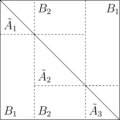
The induction strategy
-
(v)
Consider the grand sum (i.e., the sum of all entries) of a matrix
$$ \operatorname{gs}(A)=\sum_{j,k}A_{jk}. $$(5)It has a trivial upper bound
$$ \bigl\vert \operatorname{gs}(A) \bigr\vert = \bigl\vert (A\vec{1}, \vec{1}) \bigr\vert \le n \Vert A \Vert , $$(6)where \(\vec{1}\) is the all one vector. It is easy to see that for any matrix A we have
$$ \sum_{\sigma}P_{\sigma}AP_{\sigma}^{*}=(n-2)! \bigl(\operatorname{gs}(A)- \operatorname{tr}(A) \bigr)E_{0}+(n-1)!\operatorname{tr}(A)I,$$where \(E_{0}=E-I\) with E being the all one matrix and I is the identity matrix, thus straightforward estimate shows
$$ \frac{1}{n!} \biggl\Vert \sum_{\sigma}P_{\sigma}AP_{\sigma}^{*} \biggr\Vert \le c \Vert A \Vert ,$$with c being an absolute constant independent of n and A, since both \(|\operatorname{gs}(A)|\) and \(|\operatorname{tr}(A)|\) are trivially bounded by \(n\|A\|\), while \(\|E_{0}\|\le \|E\|+\|I\|\le n+1\). □

4 Applications
4.1 Optimal constants in Rademacher–Menshov inequality
The Rademacher–Menshov inequality [11, 12] states that if is an orthonormal system on some measure space \((\Omega , \mu )\) and is a scalar sequence, then
where C is independent of a, φ, n and
is often called the majorant function. With this inequality, one can further establish the Rademacher–Menshov theorem, i.e., if \(\sum_{k=1}^{\infty}|a_{k}|^{2}\ln ^{2} k<\infty \), then \(\sum_{k=1}^{\infty}a_{k}\varphi _{k}\) converges a.e. for all orthonormal systems . That boundedness of the majorant function implies a.e. convergence of the series is today a standard technique, see, e.g., the exposition in [23].
For convenience, let us denote
For fixed n, \(R_{n}\) is the optimal constant in the right-hand side of (7) (while C in the right-hand side of the Rademacher–Menshov inequality (7) upper bounds \(R_{n}\) for all n). With the help of T̃, \(R_{n}\) can be estimated as follows.
Corollary 1
For fixed n, the optimal constant \(R_{n}\) as defined in (8) in the Rademacher–Menshov inequality (7) satisfies \(R_{n}\to \frac{1}{\pi}\) as \(n\to \infty \).
Proof
Denote
That \(R_{n}\ln n=L_{n}\) can be justified in the following way (see also [13] for a different approach in probabilistic setting):
Let \(\Lambda =\{\Lambda _{j}\}_{j=1}^{n}\) be a partition of Ω where each \(\Lambda _{j}\) is μ measurable. Compose the matrix \(A^{(\Lambda )}\) whose elements are defined as
then \(A^{(\Lambda )}\) is a unitary linear map from to \(L^{2}(\Lambda _{1})\oplus L^{2}(\Lambda _{2})\oplus \cdots \oplus L^{2}( \Lambda _{n})\) since if and \(f=a_{1}\varphi _{1}+a_{2}\varphi _{2}+\cdots +a_{n}\varphi _{n}\), then
where \(L^{2}(\Lambda )\) denotes \(L^{2}(\Lambda _{1})\oplus L^{2}(\Lambda _{2})\oplus \cdots \oplus L^{2}( \Lambda _{n})\). Now take
then we have
consequently
On the other hand, consider the following particular partition:
i.e., x belongs to \(\tilde{\Lambda}_{j}\) if j is the smallest index where the sum \(|\sum_{i=1}^{j}a_{i}\varphi _{i}(x)|\) attains the value of the majorant function \(M_{n}(x)\) at x. Each \(\tilde{\Lambda}_{j}\) is also measurable, since it is the pre-image of the measurable set \(\mathrm{range}(M_{n})\) under the function mapping \(x\mapsto |\sum_{i=1}^{j}a_{i}\varphi _{i}(x)|\), thus we obtain that (with \(\|a\|=1\))
together we get that \(R_{n}=L_{n}\). It then easily follows from (2) and Theorem 1 (i) that
□
4.2 Ordering in Gauss–Seidel type methods
Let A be positive definite with diagonal D and strict lower triangular part L, then the error reduction matrix for applying the Gauss–Seidel method on a linear system \(Ax=b\) is \(Q=I-(D+L)^{-1}A\), thus with Theorem 1 (i) we can conclude that the error reduction rate per cycle is at least (see also [24])
where \(\kappa (A)\) is the spectral condition number of A and the constant c is independent of n, A and is approximately \(1/\pi \).
A similar result holds for the Kaczmarz method [25], an alternating projection method also known as ART ([26]) whose randomized version has drawn much attention in recent years since [27]. Running the Kaczmarz method on \(Ax=b\) is equivalent to running the Gauss-Seidel method implicitly on \(AA^{*}y=b\) (see [28]). The Kaczmarz method converges even for rank deficient A and inconsistent systems (see [29]), thus with Theorem 1 (iii), the error reduction rate in (9) can be improved in the rank deficient case by replacing the lnn factor with the lnr factor, the same also holds for the Gauss–Seidel method on positive semi-definite matrices.
An often observed phenomena in reality is that rearranging the ordering of equations may (though need not) accelerate the error reduction. Theorem 1 (iv) and (v) provides an explanation: The linear system in natural ordering (given ordering) may converge slowly in bad cases where the lnn factor in (9) may be active, but by (iv) there exists some good ordering with which one can get rid of this lnn factor, while (v) shows that shuffling equations after each sweep will on average also remove it.
Availability of data and materials
Not applicable.
References
King, F.: Hilbert Transform (Vol 1 and 2). Cambridge University Press, Cambridge (2009)
Carleson, L.: On convergence and growth of partial sums of Fourier series. Acta Math. 116(1), 135–157 (1966)
Hunt, R.: On the convergence of Fourier series, orthogonal expansions and their continuous analogues. In: Proceedings of the Conference at Edwardsville Ill, pp. 235–255 (1967)
Böttcher, A., Grudsky, S.: Toeplitz Matrices, Asymptotic Linear Algebra, and Functional Analysis. Springer, Berlin (2000)
Gohberg, I., Goldberg, S., Kaashoek, M.: Basic Classes of Linear Operators. Springer, Berlin (2012)
Gasch, J., Gilbert, J.: Triangularization of Hankel operators and the bilinear Hilbert transform. Contemp. Math. 247, 235–248 (1999)
Oswald, P., Zhou, W.: Convergence analysis for Kaczmarz-type methods in a Hilbert space framework. Linear Algebra Appl. 478, 131–161 (2015)
Oswald, P., Zhou, W.: Random reordering in SOR-type methods. Numer. Math. 135(4), 1207–1220 (2017)
Gohberg, I., Krein, M.: Theory and Applications of Volterra Operators in Hilbert Space. Am. Math. Soc., Providence (1970)
Davidson, K.: Nest Algebras. Longman, Harlow (1988)
Rademacher, H.: Einige Sätze über Reihen von allgemeinen Orthogonalfunktionen. Math. Ann. 87(1–2), 112–138 (1922)
Meńshov, D.: Sur les séries de fonctions orthogonales I. Fundam. Math. 4, 82–105 (1923)
Chobanyan, S., Levental, S., Salehi, H.: On the constant in Menshov–Rademacher inequality. J. Inequal. Appl. 2006, 68969 (2006)
Russo, B.: On the Hausdorff–Young theorem for integral operators. Pac. J. Math. 68(1), 241–253 (1977)
Goffeng, M.: Analytic formulas for the topological degree of non-smooth mappings: the odd-dimensional case. Adv. Math. 231(1), 357–377 (2012)
Rozenblum, G., Ruzhansky, M., Suragan, D.: Isoperimetric inequalities for Schatten norms of Riesz potentials. J. Funct. Anal. 271(1), 224–239 (2016)
Titchmarsh, E.: Introduction to the Theory of Fourier Integrals. Oxford University Press, London (1948)
Wheeden, R., Zygmund, A.: Measure and Integral. Dekker, New York (1977)
Anderson, J.: Restrictions and representations of states on \(C^{*}\) algebras. Trans. Am. Math. Soc. 249(2), 303–329 (1979)
Kadison, R., Singer, I.: Extensions of pure states. Am. J. Math. 81(2), 383–400 (1959)
Marcus, A., Spielman, D., Srivastava, N.: Interlacing families II: mixed characteristic polynomials and the Kadison–Singer problem. Ann. Math. 182(1), 327–350 (2015)
Casazza, P., Tremain, J.: Consequences of the Marcus/Spielman/Srivastava solution of the Kadison–Singer problem. In: Trends in Applied Harmonic Analysis, pp. 191–214. Springer, Berlin (2016)
Meaney, C.: Remarks on the Rademacher-Menshov Theorem. Research Symposium Asymptotic Geometric Analysis, Harmonic Analysis and Related Topics (2007)
Oswald, P.: On the convergence rate of SOR: a worst case estimate. Computing 52(3), 245–255 (1994)
Kaczmarz, S.: Angenäherte Auflösung von Systemen linearer Gleichungen. Bull. Int. Acad. Pol. Sci. Lett. 35, 355–357 (1937)
Gordon, R., Bender, R., Herman, G.: Algebraic reconstruction techniques (ART) for three-dimensional electron microscopy and X-ray photography. J. Theor. Biol. 29(3), 471–481 (1970)
Strohmer, T., Vershynin, R.: A randomized Kaczmarz algorithm with exponential convergence. J. Fourier Anal. Appl. 15(2), 262–278 (2009)
Hackbusch, W.: Iterative Solution of Large Sparse Systems of Equations. Springer, Berlin (1994)
Galantai, A.: Projectors and Projection Methods. Springer, Berlin (2004)
Acknowledgements
Not applicable.
Funding
Not applicable.
Author information
Authors and Affiliations
Contributions
The author read and approved the final manuscript.
Corresponding author
Ethics declarations
Competing interests
The author declares that they have no competing interests.
Rights and permissions
Open Access This article is licensed under a Creative Commons Attribution 4.0 International License, which permits use, sharing, adaptation, distribution and reproduction in any medium or format, as long as you give appropriate credit to the original author(s) and the source, provide a link to the Creative Commons licence, and indicate if changes were made. The images or other third party material in this article are included in the article’s Creative Commons licence, unless indicated otherwise in a credit line to the material. If material is not included in the article’s Creative Commons licence and your intended use is not permitted by statutory regulation or exceeds the permitted use, you will need to obtain permission directly from the copyright holder. To view a copy of this licence, visit http://creativecommons.org/licenses/by/4.0/.
About this article

Cite this article
Zhou, W. Properties and applications of a conjugate transform on Schatten classes. J Inequal Appl 2022, 126 (2022). https://doi.org/10.1186/s13660-022-02863-4
Received:
Accepted:
Published:
DOI: https://doi.org/10.1186/s13660-022-02863-4