A note on a mixed routing and scheduling problem on a grid graph

Abstract

We consider a particular case of the Fleet Quickest Routing Problem (FQRP) on a grid graph of m × n nodes that are placed in m levels and n columns. Starting nodes are placed at the first (bottom) level, and nodes of arrival are placed at the mth level. A feasible solution of FQRP consists in n Manhattan paths, one for each vehicle, such that capacity constraints are respected. We establish m*, i.e. the number of levels that ensures the existence of a solution to FQRP in any possible permutation of n destinations. In particular, m* is the minimum number of levels sufficient to solve any instance of FQRP involving n vehicles, when they move in the ways that the literature has until now assumed. Existing algorithms give solutions that require, for some values of n, more levels than m*. For this reason, we provide algorithm CaR, which gives a solution in a graph m* × n, as a minor contribution.

1 Introduction

In this paper, we study conditions under which the FQRP on a grid graph has a solution. A grid graph is a Manhattan graph of m × n nodes: nodes are placed in m levels and n columns. FQRP on a grid graph is a particular multi-commodity flow problem in which we must find the routes n vehicles have to perform from an initial position, at the lowest level, to a final position, at the highest level. Vehicles must respect capacity constraints on the arcs and on the nodes of the grid, i.e. at most one vehicle at a time is allowed to cross an arc or a node. The original FQRP consists in the minimization of the sum of the times necessary to route each vehicle.

In a generic graph, FQRP is an NP-complete problem. It has many applications such as the planning of land transhipment of aircraft in aprons and the building of paths for automated guided vehicles (AGV). It is evident that FQRP is a routing as well as a scheduling problem. Obviously, the specific application field determines both the formulation of the problem and the constraints on the characteristics of the paths. In Ravizza et al (2014) the problem focuses on the land movements of aircraft. It is formulated for a directed graph in which arcs represent taxiways. The aim is to minimize the overall route time, avoiding conflicts and satisfying planned take-off times on various runways.

Many authors, even though slightly modifying the hypothesis, have found solutions to the problem, using mixed integer linear programming (Roling and Visser, 2008; Gupta et al, 2009; Clare and Richards, 2011), integer programming (Smeltink and Soomer, 2005) or a linear multi-commodity flow model with side constraints and binary variables. Then, they solved the problem with Branch and Bound or Fix and Relax (Marín and Marin, 2006) techniques. Other authors (Pesic, 2001; Garcia et al, 2005; Balakrishnan and Jung, 2007; Andreatta et al, 2010) suggested various algorithms in order to solve the problem. The particular case of FQRP we are concerned with in this paper was first studied in Andreatta et al (2010) where authors state that an optimal solution to FQRP on grid graphs can be obtained routing each vehicle on a Manhattan path without stopping and avoiding conflicts between vehicles.

Furthermore, they provide a dispatching algorithm (DA) to find such a solution in polynomial time. DA finds optimal solutions in which vehicles perform all their horizontal moves on one and only one level and each level allows horizontal movements in one direction only.

It is important to stress that authors implicitly assume to deal with a graph having a number of levels high enough to allow DA find a solution, rather than define explicitly the number of levels in the instance they consider. Finally, they provide an instance dependent upper bound to number of levels needed by DA to solve an instance of FQRP.

Such a value is K ₀, namely the maximum horizontal distance of a discordant vehicle at time t = 0, i.e. when all vehicles lie on their starting nodes on the first level. A vehicle is discordant either if it has to move horizontally in a direction opposite to the one allowed by the level where the vehicle is or if it has only vertical steps remaining to perform. Thus, $K_{0} \le n - 1$.

We will consider $m_{\text{DA}}^{*} = n$ as the instance independent upper bound to the number of levels needed by DA to solve any possible instance of FQRP involving n vehicles. Considering such a value allows including also the case $n = 2$ which, strictly speaking, needs two levels. In this way, without affecting that much neither the overall results of Andreatta et al (2010) nor this work, more general results are achieved.

The main aim of this paper is to find the number of levels (m*) that ensures the existence of a solution to FQRP in each permutation of n vehicles destination. In this perspective, with respect to a specific permutation of vehicles destination, a number of levels lower than m* could be (necessary and) sufficient.

In particular, as we shall see, m* is the minimum number of levels necessary and sufficient in order to solve any instance FQRP when vehicles perform all their horizontal steps on one and only one level and each level allows horizontal movements in one direction only.

The value of m* is not instance dependent but depends on the length of what we shall call C-type conflict paths that can be found in an instance of the problem composed by n vehicles. Furthermore, we will show that $m^{*} \le m_{\text{DA}}^{*}$ for values of $n > 1$ and that the higher the value of n the higher the number of levels that can be saved with respect to pre-existing solutions.

For this reason, as the second (and minor) aim of the paper, we provide an algorithm (CaR) to find Manhattan paths of each vehicle in a graph m* × n.

The paper is structured as follows: in the next section, we recall the main elements of FQRP, while in the second we study all possible conflicts configuration. In the third, we define what a C-type conflict path is, what is its length and some general features of conflict paths.

In the fourth and in the fifth section, we deal with the main aim of the paper. The second aim of the paper is discussed in the sixth section.

In section seven we make a comparison between CaR solution and the solution obtained by executing DA, and finally we report conclusions.

2 The FQRP problem

The specific FQRP we are concerned with in this paper is related to the movements of n vehicles on an undirected grid graph or Manhattan graph, $G = \left( {V,E} \right)$. In G, we recognize m levels and n columns. V is the vertex set, while E is the set of the edges. Therefore, we have $\left| V \right| = mn$.

In the following, we assume to have a number of vehicles equal to the number of columns.

If the number of vehicles is higher than the number of columns, the problem is not feasible, while if the number of vehicles is lower than the number of columns, there are fewer conflicts between vehicles. In the last case, it is possible to find an optimal solution using CaR and considering just existing vehicles.

The n vehicles start all at time $t = 0$ from the level 1 and must reach their destination, which is known in advance, in level m. Each edge (both horizontal and vertical) requires one unit of time to be traversed. The objective of FQRP is to minimize the overall time, i.e. the sum of the time n vehicles need to perform the movement.

For the sake of simplicity, we follow the same notations used in Andreatta et al (2010). Thus, vehicles will be numbered from 1 to n and start from level 1. Their destinations correspond to a given permutation

$$ \sigma = \sigma_{1} , \sigma_{2} , \ldots , \sigma_{n} $$

of the integers from 1 to n. For practical purposes, it may also be useful to take account of the corresponding function $i \to \sigma \left( i \right)$, where $\sigma \left( i \right)$ denotes the destination column of vehicle i.

Furthermore, we will call node $\left( {p, q} \right)$ the node belonging to level p and column q.

As already stated, all vehicles start at the same time and do not stop until they reach the final destination.

In order to be feasible, the solution must not allow two vehicles to come into conflict, i.e. each arc as well as each node must be crossed by just one vehicle at a time.

For example, an instance on a Manhattan graph 5 × 5 and $\sigma_{1} = 5, \,\sigma_{2} = 4,\,\sigma_{3} = 3,\,\sigma_{4} = 1,\,\sigma_{5} = 2$, equivalent to $\sigma \left( 1 \right) = 4, \sigma \left( 2 \right) = 5, \sigma \left( 3 \right) = 3, \sigma \left( 4 \right) = 2, \sigma \left( 5 \right) = 1,$ can be represented by a figure, as shown in Figure 1.

Figure 1

FQRP instance on a Manhattan graph 5 × 5

The minimum length property of the Manhattan path of vehicle i is equivalent to the statement that, in each step, a vehicle can perform only one out of two movements: a vertical or a horizontal step. The horizontal step is towards the right if $\sigma \left( i \right) > i$ and conversely if $\sigma \left( i \right) < i.$ Paths cannot contain steps in opposite directions.

Without loss of generality, we will consider not decomposable problems in what follows. We call ‘decomposable in two (or more) disjoint subproblems’ problems in which there exists a number $k < n$ such that $\sigma \left( 1 \right), \sigma \left( 2 \right), \ldots ,\sigma \left( k \right)$ is a permutation of the integers $1, 2, \ldots , k$.

It is quite evident that, in such a case, the vehicles that occupy the positions from 1 to k in the first level must reach a destination in one of the first k columns and may be treated separately from the other vehicles.

3 Conflicts between vehicles

As we already said, the n vehicles, which have to move on paths in the Manhattan graph ($m \times n$), start from their initial position, respectively, $1, 2, \ldots , n$ in the first level and go to their respective ending positions, defined by $\sigma \left( 1 \right),\,\sigma \left( 2 \right), \ldots , \sigma \left( n \right)$.

Vehicles start simultaneously and never stop until they reach the final position. Each vehicle must move horizontally or vertically fulfilling capacity constraints on nodes and on arcs.

The number of horizontal steps for vehicle i is $\left| {\sigma \left( i \right) - i} \right|.$ As said before, if $\sigma \left( i \right) > i$, then steps are to the right while if $\sigma \left( i \right) < i$ then steps are to the left. A vehicle must perform only vertical steps iff $\sigma \left( i \right) = i$.

It is quite natural to partition the set of vehicles in three subsets:

$$ R_{1} = \{vehicles\,i |\sigma \left( i \right) > i\} $$

$$ L_{1} = \{vehicles\,i |\sigma \left( i \right) < i\} $$

$$ H = \{vehicles\,i |\sigma \left( i \right) = i\} $$

Of course, the units of time needed in order to be sure that each vehicle reaches its destination is equal to T, where T is:

$$ T = \mathop {\hbox{max} }\limits_{i} \left| {\sigma \left( i \right) - i} \right| + m $$

The last expression allows us to explain why, in some real applications, the value of m is important: such a number affects both T and the existence of a solution. As a consequence, the value of m should be minimum but high enough to guarantee the existence of a solution.

Considering a graph $m^{*} \times n$ allows reducing the effort, in terms of time, to route all vehicles to their destinations. For each couple of vehicles i and j, with $i < j$, starting at time 0 from nodes at the first level, we can have exactly one of the following:

• 1. $i \in H , j \in H$

• 2. $i \in H$ and $j$ must perform at least a horizontal step:

  • a. $\sigma \left( i \right) < \sigma \left( j \right)$

  • b. $\sigma \left( i \right) > \sigma \left( j \right)$

• 3. $j \in H$ and $i$ must perform at least a horizontal step:

  • a. $\sigma \left( i \right) < \sigma \left( j \right)$

  • b. $\sigma \left( i \right) > \sigma \left( j \right)$

• 4. $i \in R_{1} , j \in R_{1}\, or\, i \in L_{1} , j \in L_{1}$:

  • a. $\sigma \left( i \right) > \sigma \left( j \right)$

  • b. $\sigma \left( i \right) < \sigma \left( j \right)$

• 5. $i \in R_{1} , j \in L_{1} :$

  • a. $\sigma \left( i \right) < \sigma \left( j \right)$

  • b. $\sigma \left( i \right) > \sigma \left( j \right)$

    • $\frac{i + j}{2}$ is not integer

    • $\frac{i + j}{2}$ is integer and $\sigma \left( i \right) \ne \frac{i + j}{2} \ne \sigma \left( j \right)$

    • $\frac{i + j}{2}$ is integer and $\sigma \left( i \right) = \frac{i + j}{2}$ or $\sigma \left( j \right) = \frac{i + j}{2}$.

• 6. $i \in L_{1} , j \in R_{1}$

In the first case, both vehicles have only vertical moves: they cannot collide.

In cases 2.a. and 3.a., column $i = \sigma \left( i \right)$ is not between columns j and $\sigma \left( j \right)$. It follows that shortest paths of vehicles will never share any node at any time. In cases 2.b., i.e. when $i = \sigma \left( i \right)$ is between columns j and $\sigma \left( j \right)$, and 4.a, when $i \in L_{1} , j \in L_{1}$, vehicle i reaches its destination before vehicle j and stays in it in the following units of time. Then, a conflict arises only if the path of vehicle j contains the node $\left( {m,\sigma \left( i \right)} \right)$. A very similar conflict arises in cases 3.b. and 4.a., when $i \in R_{1}$, $j \in R_{1}$, in which vehicle j reaches its destination before vehicle i and stays in it in the following time units: a conflict occurs only if the path of vehicle i contains the node $\left( {m,\sigma \left( j \right)} \right)$. We will call cases 2.b., 3.b. and 4.a ‘type A conflicts’ and give the following definition:

Definition 1

Node conflicts: type A

Two vehicles i and j are subject to an A-type conflict if the following relations hold:

$$ i < j \le \sigma \left( j \right) < \sigma \left( i \right)\quad {\text{or}}\quad \sigma \left( j \right) < \sigma \left( i \right) \le i < j $$

Observation 1

The only node where a conflict between i and j may occur is the node $\left( {m, \sigma \left( j \right)} \right)$ in the first case and the node $\left( {m, \sigma \left( i \right)} \right)$ in the second one. Indeed, in both cases there is not a node belonging to a level lower than m that can be reached at the same time by the two vehicles. As a consequence, to avoid the conflict due to the occurrence of an A-type conflict, it is necessary that the destination node of j (or, in the second case, i) does not belong to path of vehicle i (or j).

Observation 2

A-type conflict is the only type of conflict that vehicles of the set H can be involved in.

In cases 4.b., 5.a. and 6, there is no conflict. Indeed, both shortest paths of the two vehicles do not share the same node or arc at the same time. In particular, in case 6, the two vehicles, i and j, never cross the same arc or node, since the left one (i.e. i) goes to the left while the right one (i.e. j) goes to the right.

In the remaining cases, i.e. the three 5.b. subcases, i and j have to perform horizontal movements in opposite directions and they can meet halfway. In these cases, they can collide on a node (or an arc) when that node (or that arc) is reachable from the departure nodes i and j after the same number of steps and when both vehicles have to pass through it. Therefore, we define three other types of conflicts, as follows.

Definition 2

Arc conflicts

Two vehicles, i and j, where $i < j$, $i \in R_{1}$, $j \in L_{1}$, are ‘subject to an arc conflict’ if we contemporarily have:

$$ \left\{ {\begin{array}{*{20}l} {i < \sigma (i)} \hfill \\ {j > \sigma (j)} \hfill \\ {\sigma (j) < \frac{i + j}{2} < \sigma (i)} \hfill \\ {j - i = 2p + 1\quad p \ge 0,\,{\text{integer}}} \hfill \\ \end{array} } \right. $$

That is to say, if vehicles i and j move horizontally one towards the other on the same level, then they enter in conflict on one of the arcs joining a node of column $\frac{i + j}{2} - 1$ with a node of column $\frac{i + j}{2} + 1$.

Definition 3

Node conflicts: type B.

We have B-type conflicts when two vehicles, i and j, $i < j$, must move in opposite direction and the following conditions hold:

$$ \left\{ {\begin{array}{*{20}l} {i < \sigma (i)} \hfill \\ {j < \sigma (j)} \hfill \\ {\sigma (j) < \frac{i + j}{2} < \sigma (i)} \hfill \\ {j - i = 2p\quad p \ge 0,\,{\text{integer}}} \hfill \\ \end{array} } \right. $$

i.e. when the horizontal distance between i and j starting nodes is an even number and the destinations of i and j are located, respectively, to the right and to the left of the median node $\left( {i + j} \right)/2$.

Observation 3

Any routing rule that allows movements only in one direction at a fixed level makes both arc conflicts and B-type conflicts impossible (and, for this reason, their determination is superfluous).

Definition 4

Node conflicts: type C

We have C-type conflicts if two vehicles i and j, with $i < j$, move in opposite direction at the same level and one of the following relations holds:

$$ \left\{ {\begin{array}{*{20}l} {\sigma \left( i \right) = \frac{{\left( {i + j} \right)}}{2}} \hfill \\ {\sigma \left( j \right) < \frac{{\left( {i + j} \right)}}{2}} \hfill \\ \end{array} } \right. $$

or, alternatively,

$$ \left\{ {\begin{array}{*{20}l} {\sigma \left( j \right) = \frac{{\left( {i + j} \right)}}{2}} \hfill \\ {\sigma \left( i \right) > \frac{{\left( {i + j} \right)}}{2}} \hfill \\ \end{array} } \right. $$

In such a framework, we define ‘vehicle subject to C-type conflict’ the vehicle whose destination is a node of the column $\left( {i + j} \right)/2$. In order to express this relation between vehicles i and j, we use the notation $i\left( j \right)$ if $\sigma \left( i \right) = \left( {i + j} \right)/2$; otherwise, we write $j\left( i \right)$ if $\sigma \left( j \right) = \left( {i + j} \right)/2$.

The following proposition holds.

Proposition 1

In order to avoid the collision which could arise from the occurrence of $i\left( j \right)$, when $i < j$, the first node of column $\sigma \left( i \right)$ belonging to the path of vehicle $i$ must be $\left( {q, \sigma \left( i \right)} \right)$ and the last node of the same column belonging to the path of vehicle $j$ must be $\left( {p, \sigma \left( i \right)} \right)$, with $q > p$.

Proof

If we have $i$ and $j$, with $i < j$ and $i\left( j \right),$ it follows that:

$$ \sigma \left( i \right) = \frac{{\left( {i + j} \right)}}{2}\quad {\text{and}}\quad \sigma \left( j \right) < \sigma \left( i \right) $$

Therefore, column $\sigma \left( i \right)$, which is the one containing the destination node of vehicle $i$, is equidistant from the columns from which $i$ and $j$ start:

$$ \sigma \left( i \right) - i = j - \sigma \left( i \right) $$

We distinguish two cases:

• If $q \le p$ then both vehicles reach the node $\left( {p, \sigma \left( i \right)} \right)$ at time $t = \frac{j - i}{2} + p - 1$. In fact, remembering that they are equidistant from column $\sigma \left( i \right)$, if $q = p$ then both vehicles are on the node $\left( {p, \sigma \left( i \right)} \right)$ at the same time. On the other side, if $q < p$, then vehicle $i$ reaches column $\sigma \left( i \right)$ at time $t = \frac{j - i}{2} + q - 1$ and it has only vertical steps left. Moving vertically in the following time units, it occupies the nodes from $\left( {q + 1, \sigma \left( i \right)} \right)$ to $\left( {p, \sigma \left( i \right)} \right)$ and so $j$ cannot avoid to use a node in which vehicle $i$ is still.

• If $q > p$, then vehicle $j$ leaves the column $\sigma \left( i \right)$ before than the arrival of vehicle $i$, i.e. at time $t = \frac{j - i}{2} + p - 1$. In this way, the occurrence of a conflict is avoided (Figure 2).□

  Figure 2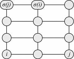

  

  An example of C-type conflict

Observation 4

In order to discover C-type conflicts, we need $O\left( n \right)$ calculations. Indeed, it is sufficient to scan all vehicles and verify what follows:

• If $i = \sigma \left( i \right),$ $i$ cannot be subject to C-type conflict;

• If $i < \sigma (i$), then find the vehicle $j = 2 \sigma \left( i \right) - i$: we have a C-type conflict $i\left( j \right)$ iff $\sigma \left( j \right) < \left( {i + j} \right)/2$;

• If $i > \sigma (i$), then find the vehicle $j = 2 \sigma \left( i \right) - i$: we have a C-type conflict $i\left( j \right)$ iff $\sigma \left( j \right) > \left( {i + j} \right)/2$.

Observation 5

The conflict relation $u\left( v \right)$ is asymmetric because when vehicle $u$ is subject to C-type conflict with vehicle $v$, $v$ cannot be subject to C-type conflict with $u$. Furthermore, it is univocal because it is impossible to simultaneously have two relations $u\left( v \right)$ and $u\left( w \right)$ with $v \ne w$.

Consequently, we can represent C-type conflicts in an instance FQRP by a directed graph $G^{{\prime }} = \left( {N^{{\prime }} ,A^{{\prime }} } \right)$ in which nodes represent vehicles and the generic arc $\left( {u, v} \right)$ represents the relation $u\left( v \right)$.

Conflict graph $G^{{\prime }}$ is a family of arborescences. Arcs are oriented towards the root: for each node, the outer degree is at most 1 (the inner degree can be higher than 1).

4 Paths of C-type conflicts

We call C-type conflict path (more simply, conflict path), any sequence of vehicles $\left\{ {z_{1} ,z_{2} , \ldots , z_{k} } \right\}$ that generates a number $k$ of C-type conflicts $z_{1} \left( {z_{2} } \right),z_{2} \left( {z_{3} } \right), \ldots ,z_{k} \left( {z_{k + 1} } \right)$: in short these vehicles constitute the path $\left( {z_{1} ,z_{2} , \ldots ,z_{k} } \right)$. As a particular case, a conflict path can consist of a single C-type conflict: $z_{1} \left( {z_{2} } \right).$ In graph $G^{{\prime }}$, the conflict path $\left( {z_{1} ,z_{2} , \ldots ,z_{k} } \right)$ corresponds to a (directed) path from node $z_{1}$ to node $z_{k}$. Based on the previous definitions, it is evident that in a path of conflicts, vehicles $z_{i} , i\,{\text{odd}}$ must move in opposite direction with respect to vehicles $z_{j} , j {\text{even}}$.

Definition 5

Length of a path

We define Length of a path the number of vehicles subject to the C-type conflict in a path. In other words, the length of the generic conflict path $z_{1} \left( {z_{2} } \right),z_{2} \left( {z_{3} } \right), \ldots ,z_{k} \left( {z_{k + 1} } \right)$ is k.

Observation 6

Conflict paths allow building a list of priorities that must be respected. Consider a C-conflict path such that relations $z_{1} \left( {z_{2} } \right), z_{2} \left( {z_{3} } \right)$ hold. Proposition 1 allows us to state that both paths of vehicles $z_{1}$ and $z_{2}$ contain at least a node of column $\sigma \left( {z_{1} } \right)$ and that both paths of vehicles $z_{2}$ and $z_{3}$ contain at least a node of column $\sigma \left( {z_{2} } \right)$. Proposition 1 follows that the first node of column $\sigma \left( {z_{1} } \right)$ belonging to the path of $z_{1}$ must be located on $h_{{z_{1} }} > h_{{z_{2} }}^{{\prime }}$, where $h_{{z_{2} }}^{{\prime }}$ is the level of the last node of column $\sigma \left( {z_{1} } \right)$ belonging to the path of $z_{2}$.

Similarly, the first node of column $\sigma \left( {z_{2} } \right)$ belonging to the path of $z_{2}$ must be located on a level $h_{{z_{2} }} > h_{{z_{3} }}^{{\prime }}$, where $h_{{z_{3} }}^{{\prime }}$ is the level of last node of column $\sigma \left( {z_{2} } \right)$ belonging to the path of $z_{3}$.

Obviously, it is $h_{{z_{2} }} \ge h_{{z_{2} }}^{{\prime }}$. Indeed, column $\sigma \left( {z_{1} } \right)$ must be located between $z_{2}$ and $\sigma \left( {z_{2} } \right)$. As a consequence, when $z_{2}$ reaches the node $\left( {h_{{z_{2} }}^{{\prime }} ,\sigma \left( {z_{1} } \right)} \right)$, two are the cases: if $z_{2}$ does not perform any vertical steps in the section of its paths from column $\sigma \left( {z_{1} } \right)$ to column $\sigma \left( {z_{2} } \right)$, then it must be $h_{{z_{2} }} = h_{{z_{2} }}^{{\prime }}$. Otherwise, i.e. if $z_{2}$ performs one or more vertical steps in such a section, it must be $h_{{z_{2} }} = h_{{z_{2} }}^{{\prime }}$.

Thus, referring to a conflict path whose length is $k$, called $h_{{z_{i} }}$ the level of first node of column $\sigma \left( {z_{i} } \right)$ belonging to the path of $z_{i}$ and $h'_{{z_{i} }}$ the level of the last node of column $\sigma \left( {z_{i - 1} } \right)$ belonging to the path of $z_{i}$ the following relations hold:

$$ h_{{z_{i} }} > h_{{z_{i + 1} }}^{{\prime }} \quad i = 1, \ldots ,k $$

$$ h_{{z_{i} }} \ge h_{{z_{i} }}^{{\prime }} \quad i = 2, \ldots ,k + 1 $$

These relations represent a list of priorities that must be respected (in order to find a feasible solution to FQRP).

Observation 7

$k + 1$ levels are sufficient to route the vehicles belonging to a conflict path whose length is $k$.

Indeed, these $k + 1$ vehicles could be routed using a very simple rule: each vehicle performs all its horizontal steps on one and only one level (opportunely chosen respecting the previously shown list of priorities) and each level allows performing its horizontal steps to one and only one of these vehicles. The result is an 1-1 assignment of vehicles to levels, so that $k + 1$ levels are required and sufficient. Note that the spirit of the previous rule is quite similar to the one of the DAs: in both vehicles performs all their horizontal steps on one and only one level and each level allows movement in one direction only. These rules imply that $h_{{z_{i} }} = h_{{z_{i} }}^{{\prime }}$ for each i. Then, we could write the second relation shown in Observation 6 as follows:

$$ h_{{z_{i} }} > h_{{z_{i + 1} }} \quad i = 1, \ldots ,k $$

i.e. if each vehicle performs all its horizontal steps on one and only one level and each level allows movements in one direction only, $z_{k + 1}$ levels are necessary and sufficient to route all vehicles belonging to a conflict path whose length is k.

Finally, Proposition 2 states a general property of conflict paths.

Proposition 2

Given a path $z_{1} \left( {z_{2} } \right),z_{2} \left( {z_{3} } \right), \ldots ,z_{k} \left( {z_{k + 1} } \right)$, the distance $\left| {z_{k + 1} - z_{k} } \right|$ is higher than the distance between any other couple of vehicles belonging to the conflict path.

Proof

Assume that $z_{i} - \sigma \left( {z_{i} } \right) < 0$ if $i$ is odd and $z_{i} - \sigma \left( {z_{i} } \right) > 0$ otherwise. Then it must be:

$$ \begin{array}{*{20}c} {\sigma \left( {z_{1} } \right) > \sigma \left( {z_{2} } \right)} \\ {\sigma \left( {z_{2} } \right) < \sigma \left( {z_{3} } \right)} \\ {\sigma \left( {z_{3} } \right) > \sigma \left( {z_{4} } \right)} \\ {\sigma \left( {z_{4} } \right) < \sigma \left( {z_{5} } \right)} \\ \ldots \\ \end{array} $$

where the last inequality is $\sigma \left( {z_{k - 1} } \right) > \sigma \left( {z_{k} } \right)$ if $k$ is even and it is $\sigma \left( {z_{k - 1} } \right) < \sigma \left( {z_{k} } \right)$ otherwise.

Remembering that in the considered path $\sigma \left( {z_{i} } \right) = \frac{{z_{i} + z_{i + 1} }}{2}$, substituting such values in the previous inequalities we obtain:

$$ z_{k} < \cdots < z_{5} < z_{3} < z_{1} \,{\text{and}}\,z_{2} < z_{4} < z_{6} < \cdots < z_{k + 1} $$

if $k$ is even, and

$$ z_{k + 1} < \cdots < z_{5} < z_{3} < z_{1} \,{\text{and}}\,z_{2} < z_{4} < z_{6} < \cdots < z_{k} $$

otherwise.

Since $z_{1} \left( {z_{2} } \right)$ and $z_{1} \in R_{1}$, it must necessarily be $z_{1} < z_{2}$. As a consequence, it will be:

$$ z_{k} < \cdots < z_{5} < z_{3} < z_{1} < z_{2} < z_{4} < z_{6} < \cdots < z_{k + 1} $$

if k is even, and

$$ z_{k + 1} < \cdots < z_{5} < z_{3} < z_{1} < z_{2} < z_{4} < z_{6} < \cdots < z_{k} $$

if $k$ is odd. Note that $z_{k}$ and $z_{k + 1}$ are, respectively, the leftmost and rightmost elements in the first case and the rightmost and leftmost elements in the second case. This proves the thesis. To prove the other case, i.e. when $z_{i} - \sigma \left( {z_{i} } \right) > 0$ if $i$ is odd and $z_{i} - \sigma \left( {z_{i} } \right) < 0$ otherwise, it is sufficient to repeat the above-mentioned procedure considering that all the inequalities that holds in the previous case are reversed.□

Corollary 1

A conflict path whose length is $k$ needs at least $\left| {z_{k + 1} - z_{k} } \right| + 1$ columns to exist.

5 The relation between the length of the C-conflict path and number of vehicles in the graph

In this section, we establish the relation between the length k of a conflict path and the minimum number of columns (and, consequently, vehicles) needed to guarantee the existence of such a path, i.e. $z_{1} (z_{2} ), z_{2} (z_{3} ), \ldots ,z_{k} \left( {z_{k + 1} } \right)$. In other words, with regard to all possible permutations which contain a conflict path whose length is $k$, we find the number of columns of the permutation composed by the minimum number of vehicles.

Then, to find such a number, which we shall call $n_{ \hbox{min} }$, we solve the following problem:

$$ \mathop {\text{min }}\limits_{{\varSigma^{\left( k \right)} }} \left\{ {\left| {z_{k + 1} - z_{k} } \right| + 1} \right\} $$

where $\left| {z_{k + 1} - z_{k} } \right| + 1$ is the number of column needed to a conflict path whose length is $k$ to exist (see Corollary 1) and $\varSigma^{\left( k \right)}$ is the set of all permutations which contain a $k$ length conflict path. Consequently, $n_{min}$ is the value of the objective function in correspondence of an optimal solution.

Proposition 3 allows decomposing objective function of the previous problem in a very useful way.

Proposition 3

Consider a conflict path whose length is $k$. Then, the following holds:

$$ \left| {z_{k} - z_{k + 1} } \right| = 2\left( {\left| {z_{1} - \sigma \left( {z_{1} } \right)} \right| + \mathop \sum \limits_{i = 1}^{k - 1} \left| {\sigma \left( {z_{i} } \right) - \sigma \left( {z_{i + 1} } \right)} \right|} \right) $$

Proof

In the following, without loss of generality, we assume that $z_{i} - \sigma \left( {z_{i} } \right) < 0$ if $i$ is an odd number, while it will be $z_{i} - \sigma \left( {z_{i} } \right) > 0$ otherwise. First, we prove the proposition assuming $k$ an odd number.

In this case, $\left| {z_{k} - z_{k + 1} } \right| = z_{k + 1} - z_{k}$, and keeping in mind:

$$ z_{h + 1} - z_{h} = 2\left[ {\sigma \left( {z_{h} } \right) - z_{h} } \right],\forall h, $$

we can write:

$$ \begin{aligned} z_{k + 1} - z_{k} & = 2\left[ {\sigma \left( {z_{k} } \right) - z_{k} } \right] \\ & = 2\left[ {\sigma \left( {z_{k} } \right) - z_{k} + z_{k - 1} - z_{k - 1} + z_{k - 2} - z_{k - 2} + \cdots + z_{2} - z_{2} + z_{1} - z_{1} } \right] \\ & = 2\left[ {\left( {\sigma \left( {z_{k} } \right) - \sigma \left( {z_{k - 1} } \right)} \right) + \left( {\sigma \left( {z_{k - 2} } \right) - \sigma \left( {z_{k - 1} } \right)} \right) + \cdots + \left( {\sigma \left( {z_{1} } \right) - \sigma \left( {z_{2} } \right)} \right) + \left( {\sigma \left( {z_{1} } \right) - z_{1} } \right) } \right] \\ \end{aligned} $$

Since k is odd, and given that $z_{i} \in R_{1}$ if i is an odd number while it belongs to $L_{1}$ otherwise, it must be:

$$ \sigma \left( {z_{1} } \right) > \sigma \left( {z_{2} } \right), \sigma \left( {z_{3} } \right) > \sigma \left( {z_{2} } \right), \sigma \left( {z_{3} } \right) > \sigma \left( {z_{4} } \right), \ldots , \sigma \left( {z_{k} } \right) > \sigma \left( {z_{k - 1} } \right) $$

As a consequence, all the terms inside round brackets are positive and this proves the thesis.

When $k$ is even, the proof is quite similar.

The other case, i.e. when we have $z_{i} - \sigma \left( {z_{i} } \right) > 0$ if i is an odd number and $z_{i} - \sigma \left( {z_{i} } \right) < 0$ otherwise, can be proved with analogous considerations.□

Observation 8

Proposition 3 shows that $\left| {z_{k} - z_{k + 1} } \right|$ is a strictly increasing function of both the sum of the distances between destinations of two consecutive vehicles in the conflict path, i.e. $\mathop \sum \limits_{i = 1}^{k - 1} \left| {\sigma \left( {z_{i} } \right) - \sigma \left( {z_{i + 1} } \right)} \right|$, and the number of horizontal steps of vehicle $z_{1}$. This leads to two considerations. First, rather than minimizing $|z_{k} - z_{k + 1} |$, we can minimize the right-hand side of equation in Proposition 3. Second, to minimize $\left| {z_{1} - \sigma \left( {z_{1} } \right)} \right|$ is trivial, since the minimum number of horizontal steps of a vehicle is 1 and it is equivalent to state that $\left| {z_{1} - z_{2} } \right| = 2$. Such a value represents the minimum distance between vehicles that can be involved in a conflict path whose length is 1, i.e. $n_{min} = 3,$ when $k = 1$. It follows that if $z_{1}$ moves towards the right, then $z_{2} = z_{1} + 2$. Otherwise it will be $z_{1} = z_{2} - 2$. Note that minimizing such a distance does not affect the minimization of $\sum\nolimits_{i = 1}^{k - 1} {\left| {\sigma \left( {z_{i} } \right) - \sigma \left( {z_{i + 1} } \right)} \right|}$.

Once proved that finding $n_{ \hbox{min} }$ when $k = 1$ it is quite trivial, in the following we focus on $k \ge 2$ assuming that $\left| {z_{1} - \sigma \left( {z_{1} } \right)} \right| = 1$. Then we will proceed as follows: first, we define a new problem which is equivalent to $\hbox{min} \left| {z_{k + 1} - z_{k} } \right| + 1$. Second, in Propositions 4 and 5 we describe properties that allow identifying whether a solution of such a new problem is optimal. Proposition 6 shows the existence, for each $k$, of a solution that has such properties.

In order to get $n_{ \hbox{min} }$, we solve the problem consisting in the determination of $k$ different destinations of vehicles, i.e. $\sigma \left( {z_{i} } \right),i = 1, \ldots ,k$, which do not overlap and minimize the following:

$$ \left| {z_{k} - z_{k + 1} } \right| = 2\left( {\mathop \sum \limits_{i = 1}^{k - 1} \left| {\sigma \left( {z_{i} } \right) - \sigma \left( {z_{i + 1} } \right)} \right| + 1} \right) $$

(1)

For the sake of simplicity, we will use the notation $\Delta_{i} = \left| {\sigma \left( {z_{i} } \right) - \sigma \left( {z_{i + 1} } \right)} \right|$.

In this way, the problem of finding the minimum number of columns that allows a k length conflict path is equivalent to find an 1-1 assignment of k vehicles to $k$ destinations for which is a minimum the quantity:

$$ \mathop \sum \limits_{i = 1}^{k - 1} \Delta_{i} $$

(2)

Note that, when $k = 2$ the problem is trivial, since we must find the min value of $\Delta_{1}$, subject to the constraint of $\Delta_{1} \ge 1$, in order to avoid that $\sigma \left( {z_{1} } \right) = \sigma \left( {z_{2} } \right)$: consequently, the optimal solution, when $k = 2$, is $\Delta_{1} = 1$.

Observation 9

In the following propositions, when we make a statement regarding the destinations of the vehicles in a conflict path, we assume given an assignment (obviously without overlapping) of the destinations of vehicles not belonging to the conflict path to the remaining columns.

Proposition 4

In the solution that minimizes (2), the destinations $\sigma \left( {z_{i} } \right), i = 1, \ldots , k$, of the vehicles involved in a conflict path of length $k$, must be located in a subset of adjacent columns of the graph.

Proof

Assume that in a feasible solution exist two vehicles destinations $\sigma \left( {z_{i} } \right)$ and $\sigma \left( {z_{j} } \right)$ situated in two non-adjacent columns, i.e. $\sigma \left( {z_{i} } \right) = p$ and $\sigma \left( {z_{j} } \right) = p + q$, with $q \ge 2$ and assume also that columns $p + 1,p + 2, \ldots ,p + q - 1$ are not destinations of any one of the vehicles involved in the conflict path.

For the sake of simplicity, we call $\varPhi = \left\{ {p + 1,p + 2, \ldots p + q - 1} \right\}$ the set of these adjacent columns.

From the assumptions, it follows that it must exist at least an integer $h$, $1 \le h \le k - 1$, such that the columns of the set $\varPhi$ are located between destinations of two consecutive vehicles $\sigma \left( {z_{h} } \right)$ and $\sigma \left( {z_{h + 1} } \right)$: if not, the hypothesis is denied, since all destinations of vehicles would be necessarily on the same side of $\varPhi$. Thus, we can move towards left, of $q - 1$ steps, all the destinations situated on columns whose index is at least $p + q$. Such movement reduces of $q - 1$ units the distance between two consecutive vehicles that are separated by $\varPhi$ and does not affect the other distances between consecutive vehicles belonging to the conflict path. It follows that any solution in which destinations of vehicles belonging to conflict path are not located in a subset of adjacent columns of the graph is not optimal.□

Now let us denote with $w_{k} = \sum\nolimits_{i = 1}^{k - 1} {\Delta_{i} }$ and $w_{k}^{*} = \hbox{min} \sum\nolimits_{i = 1}^{k - 1} {\Delta_{i} }$, respectively, the value of (2) in correspondence of a generic feasible solution—not necessarily the optimal one—and its optimal value when the path length is $k$. Proposition 5 holds.

Proposition 5

For any value of $k$, the following relation holds:

$$ w_{k}^{*} - w_{k - 1}^{*} \ge 2 $$

(3)

Proof

Consider a $k$-length C-conflict path, i.e. $z_{1} \left( {z_{2} } \right),z_{2} \left( {z_{3} } \right), \ldots ,z_{k} \left( {z_{k + 1} } \right)$. From Proposition 4, it follows that the destinations of such vehicles will identify a subset of $k$ adjacent columns of the graph. Assuming that $z_{i} - \sigma \left( {z_{i} } \right) < 0$ if $i$ is odd, while it will be $z_{i} - \sigma \left( {z_{i} } \right) > 0$, a feasible solution of (1) must respect the following inequalities:

$$ \begin{array}{*{20}c} {\sigma \left( {z_{1} } \right) > \sigma \left( {z_{2} } \right)} \\ {\sigma \left( {z_{2} } \right) < \sigma \left( {z_{3} } \right)} \\ {\sigma \left( {z_{3} } \right) > \sigma \left( {z_{4} } \right)} \\ {\sigma \left( {z_{4} } \right) < \sigma \left( {z_{5} } \right)} \\ \ldots \\ \end{array} $$

where the last inequality is $\sigma \left( {z_{k - 1} } \right) > \sigma \left( {z_{k} } \right)$ if $k$ is even and it is $\sigma \left( {z_{k - 1} } \right) < \sigma \left( {z_{k} } \right)$ otherwise.

Given an optimal solution, i.e. the permutation of $k$ destinations of vehicles belonging to the conflict path that minimizes the (1) considers in it the position of $\sigma \left( {z_{k} } \right).$ We have two cases: either $\sigma \left( {z_{k} } \right)$ is inner in the permutation, i.e. relation $\sigma \left( {z_{i} } \right) < \sigma \left( {z_{k} } \right) < \sigma \left( {z_{j} } \right)$ holds, or $\sigma \left( {z_{k} } \right)$ is the extremity of the permutation, i.e. either $\sigma \left( {z_{i} } \right) < \sigma \left( {z_{k} } \right)$ or $\sigma \left( {z_{i} } \right) > \sigma \left( {z_{k} } \right)$, $i = 1, \ldots ,k - 1$ holds. In every case, if we delete $\sigma \left( {z_{k} } \right)$ from the solution (and we delete also $_{k - 1}$ from the objective function) the remaining destinations of the vehicles $z_{1} ,z_{2} , \ldots ,z_{k - 1}$ give a feasible solution of the problem related to a path of $k - 1$ conflicts. Let us consider separately the two cases.

In the first case, $\sigma \left( {z_{k} } \right)$ is inner in the permutation, i.e. relation $\sigma \left( {z_{i} } \right) < \sigma \left( {z_{k} } \right) < \sigma \left( {z_{j} } \right)$ holds for some $z_{i}$ and $z_{j}$ belonging to the conflict path. Then, the elimination of $\sigma \left( {z_{k} } \right)$ has two effects.

The first one is the reduction in the value of (2) in the case the path length is $k - 1$ of at least one unit. Such a reduction is due to the elimination from the objective function of the addend $\Delta_{k - 1}$.

The second effect is the creation of an empty space between destinations of the remaining $k - 1$ vehicles. As a consequence, it is possible to fill such a space (see Proposition 4) in order to get adjacent destinations of vehicles belonging to the conflict path with a reduction in the objective function of at least one unit and relation (3) holds.

In the second case, when $\sigma \left( {z_{k} } \right)$ is the extremity of the permutation, as said before, either $\sigma \left( {z_{i} } \right) < \sigma \left( {z_{k} } \right)$ or $\sigma \left( {z_{i} } \right) > \sigma \left( {z_{k} } \right)$, $i = 1, \ldots ,k - 1$ holds. The first situation is possible only when $k$ is even, while the second one is possible only when $k$ is odd. Assume that $\sigma \left( {z_{k} } \right)$ is the leftmost destination of the permutation, i.e. that $k$ is even. Then, it must be:

$$ \sigma \left( {z_{k} } \right) < \sigma \left( {z_{k - 1} } \right);\sigma \left( {z_{k - 2} } \right) < \sigma \left( {z_{k - 1} } \right) $$

In order to satisfy the set of inequalities that describe a feasible solution, it must be $\Delta_{k - 1} = \left| {\sigma \left( {z_{k} } \right) - \sigma \left( {z_{k - 1} } \right)} \right| \ge 2$. Indeed, if $\Delta_{k - 1} = 1$, it would be $\sigma \left( {z_{k} } \right)$ adjacent to $\sigma \left( {z_{k - 1} } \right)$, and the only possible destination $\sigma \left( {z_{k - 2} } \right)$ available for vehicle $z_{k - 2}$ would be on the left of $\sigma \left( {z_{k} } \right)$. This would contradict the hypothesis $\sigma \left( {z_{i} } \right) > \sigma \left( {z_{k} } \right), i = 1, \ldots , k - 1$.

In this way, analogously to the procedure in Case a), we get a feasible solution for (1) when the length of the conflict path is $k - 1$, through the elimination of $\sigma \left( {z_{k} } \right)$ (and of the correspondent variable $\Delta_{k - 1}$) from the optimal solution of the conflict path whose length is $k$. It follows that the value of (2) for the $k - 1$ case in correspondence of the feasible solution obtained in this way is reduced of at least two units:

$$ w_{k - 1} \le w_{k}^{*} - 2. $$

A fortiori it will be:

$$ w_{k - 1}^{*} \le w_{k - 1} \le w_{k}^{*} - 2. $$

When $k$ is odd and $\sigma \left( {z_{k} } \right)$ is at the right extremity of the permutation, it must be:

$$ \sigma \left( {z_{k - 1} } \right) < \sigma \left( {z_{k - 2} } \right);\sigma \left( {z_{k - 1} } \right) < \sigma \left( {z_{k} } \right) $$

and very similar considerations prove that (3) holds.

The proof is quite similar when $z_{i} - \sigma \left( {z_{i} } \right) > 0$ if $i$ is odd and $z_{i} - \sigma \left( {z_{i} } \right) < 0$ otherwise.□

Observation 10

Consider $w_{k} ,$ i.e. the value of (2) in correspondence of a feasible solution—not necessarily the optimal one—when the conflict path length is $k$.

As a consequence of Proposition 5, if $w_{k} - w_{k - 1}^{*} = 2,$ then $w_{k} = w_{k}^{*}$. In other words, if $w_{k} - w_{k - 1}^{*} = 2$, then $w_{k}$ is an optimal solution of $\hbox{min} \sum\nolimits_{i = 1}^{k - 1} {\Delta_{i} }$.

Since, as said, $w_{2}^{*} = 1$, for values of $k \ge 2$ it must be $w_{k}^{*} = 2k - 3$. Substituting this value in (1) we obtain:

$$ \left| {z_{k} - z_{k + 1} } \right| = 2\left( {1 + 2k - 3} \right) = 4\left( {k - 1} \right), $$

that gives the (minimum) highest distance between vehicles belonging to the conflict path as a function of its length.

Proposition 6

A feasible solution such that $w_{k} = w_{k - 1}^{*} + 2 = 2k - 3$ exists $\forall k \ge 2$.

Proof

Consider a conflict path whose length is $k$, i.e. $z_{1} \left( {z_{2} } \right), z_{2} \left( {z_{3} } \right), \ldots , z_{k} \left( {z_{k + 1} } \right)$. In what follows we assume that $z_{i} - \sigma \left( {z_{i} } \right) < 0$ if $i$ is odd, while it will be $z_{i} - \sigma \left( {z_{i} } \right) > 0$ otherwise.

We distinguish the case in which $k$ is even and the case in which $k$ is odd. Note that in both cases, the exact destination of the vehicle $z_{k + 1}$, which do not belong to the conflict path, is irrelevant, provided that either $\sigma \left( {z_{k + 1} } \right) > \sigma \left( {z_{k} } \right)$ if $k$ is even or $\sigma \left( {z_{k + 1} } \right) < \sigma \left( {z_{k} } \right)$ if $k$ is odd.

When $k$ is even, then, as a consequence of the existence of a conflict path, it must be:

$$ \begin{array}{*{20}c} {\sigma \left( {z_{1} } \right) > \sigma \left( {z_{2} } \right)} \\ {\sigma \left( {z_{2} } \right) < \sigma \left( {z_{3} } \right)} \\ {\sigma \left( {z_{3} } \right) > \sigma \left( {z_{4} } \right)} \\ \ldots \\ {\sigma \left( {z_{k - 1} } \right) > \sigma \left( {z_{k} } \right)} \\ \end{array} $$

Then, consider the following permutation of destinations:

$$ \sigma \left( {z_{2} } \right),\sigma \left( {z_{1} } \right),\sigma \left( {z_{4} } \right),\sigma \left( {z_{3} } \right), \ldots ,\sigma \left( {z_{k} } \right), \sigma \left( {z_{k - 1} } \right). $$

The corresponding values of $\Delta_{i}$ are $\Delta_{i} = 1,\quad i = 1,3,5, \ldots ,k - 1$, and $\Delta_{i} = 3,\quad i = 2,4,6, \ldots ,k - 2$. Their sum is equal to $2k - 3$. When $k$ is odd, then it must be:

$$ \begin{array}{*{20}c} {\sigma \left( {z_{1} } \right) > \sigma \left( {z_{2} } \right)} \\ {\sigma \left( {z_{2} } \right) < \sigma \left( {z_{3} } \right)} \\ {\sigma \left( {z_{3} } \right) > \sigma \left( {z_{4} } \right)} \\ \ldots \\ {\sigma \left( {z_{k - 1} } \right) < \sigma \left( {z_{k} } \right)} \\ \end{array} $$

Then consider the following permutation of destinations:

$$ \sigma \left( {z_{2} } \right),\sigma \left( {z_{1} } \right),\sigma \left( {z_{4} } \right),\sigma \left( {z_{3} } \right), \ldots ,\sigma \left( {z_{k - 1} } \right),\sigma \left( {z_{k - 2} } \right),\sigma \left( {z_{k} } \right) $$

The corresponding values of $\Delta_{i}$ are $\Delta_{i} = 1,\quad i = 1,3,5, \ldots ,k - 2$, $\Delta_{i} = 3,\quad i = 2,4,6, \ldots ,k - 3$ and $\Delta_{k - 1} = 2$. The sum of these values is equal to $2k - 3$. □

Observation 11

Proposition 6 states the existence of an optimal solution but not necessarily it is unique. Indeed, in the other case, i.e. when $z_{i} - \sigma \left( {z_{i} } \right) > 0$ if $i$ is odd, and $z_{i} - \sigma \left( {z_{i} } \right) < 0$ otherwise, there may be other feasible solutions but, as Proposition 5 states, they cannot be better than the one presented in the proof of Proposition 6.

So, it is possible now to establish the relation between the minimum number of columns needed to the existence of a conflict and its length: recalling that $n_{\hbox{min} } = \mathop {\hbox{min} }\limits_{{\varSigma^{\left( k \right)} }} \left\{ {\left| {z_{k + 1} - z_{k} } \right| + 1} \right\}$, with $\mathop {\hbox{min} }\limits_{{\varSigma^{\left( k \right)} }} \left| {z_{k + 1} - z_{k} } \right| = 4\left( {k - 1} \right)$, $k \ge 2$, and with $\hbox{min} \left| {z_{2} - z_{1} } \right| = 2,$ we can conclude that:

$$ n_{\hbox{min} } = \left\{ {\begin{array}{*{20}l} {4k - 3} \hfill & {k \ge 2} \hfill \\ 3 \hfill & {k = 1} \hfill \\ \end{array} } \right. $$

6 The computation of the number of levels that ensure the existence of a solution to any instance of FQRP involving n vehicles

In this paragraph, we determine the number of levels that ensure the existence of a solution to any possible permutation of vehicles destinations when the value of n is fixed. In order to do so, we firstly prove that, given n, the length of the longest C-type conflict path can be computed in advance. The following proposition provides the relation between n and such a length.

Proposition 7

The length of the longest C-type conflict path in a graph $m \times n$, which we shall call $k_{\hbox{max} }$, is:

$$ k_{\hbox{max} } = \left\{ {\begin{array}{*{20}l} {1 + \text{int} \left( {\frac{n - 1}{4}} \right)} \hfill & {{\text{if}}\,n \ge 3} \hfill \\ 0 \hfill & {\text{Otherwise}} \hfill \\ \end{array} } \right. $$

where $\text{int} \left( x \right)$ is the integer part of $x$.

Proof

The result is immediately deducible considering that:

$$ n_{\hbox{min} } = \left\{ {\begin{array}{*{20}l} {4k - 3} \hfill & {k \ge 2} \hfill \\ 3 \hfill & {k = 1} \hfill \\ \end{array} } \right. $$

□

If the maximum possible length of a conflict path having $n$ vehicles is known, we can also determine the number of levels that ensure the existence of a solution to any instance of FQRP involving $n$ vehicles. We call such a number $m^{*}$, as the following proposition states.

Proposition 8

A solution to FQRP for any possible permutation of $n$ destinations $\sigma = \sigma \left( 1 \right),\sigma \left( 2 \right), \ldots ,\sigma \left( n \right)$ can be found in a graph composed of at most $m^{*}$ levels, where:

$$ m^{*} = k_{\hbox{max} } + 2 $$

Proof

We can distinguish two cases: $1 \le n \le 2$ and $n \ge 3$.

In the first case, all the permutations of destinations do not allow the existence of A-type conflicts and C-type conflicts, i.e. $k_{\hbox{max} } = 0$. In particular, when $n = 1$ we have only one vehicle that belongs to set $H$. When $n = 2$, if both vehicles do not belong to set $H$, the leftmost vehicle belongs to set $R_{1}$ while the other belongs to $L_{1}$.

In such a case, we can route all vehicles using two levels. Indeed, if the two vehicles perform all their horizontal steps on different levels, they will never enter into conflict. Note that in such a case permutations of destinations exclude the occurrence of an A-type conflict. This proves the thesis in the first case.

When $n \ge 3$, we can have no C-type conflicts as well as one or more than one conflict path, whose length is at most $k_{\hbox{max} }$.

In the absence of C-type conflicts, it is possible once more to route all vehicles using two levels: we could force vehicles belonging to a set (equivalently, $R_{1}$ or $L_{1}$) to perform all their horizontal steps on the first level while other vehicles perform all their horizontal moves on the second level. The use of such a routing rule always ensures to avoid the occurrence of any kind of conflict. Arc and B-type conflict occurrences are avoided due to the assignment to different levels of vehicles that must move in opposite directions (see Observation 3). Any possible A-type conflict is avoided (remember: when $n \ge 3$), because $m^{*} \ge 3$ and there is not a vehicle which must perform its horizontal steps on level $m^{*}$. This proves the thesis when $n \ge 3$ and $k_{ \hbox{max} } = 0$.

Alternatively, as said, we can find one or more than one conflict paths whose length is $k_{\hbox{max} }$.

In order to take advantage of Observation 7, in the following part of the proof we will assume that each vehicle performs all its horizontal steps on one and only one level. This implies that it must be $h_{{z_{i} }} > h_{{z_{i + 1} }}$ for each vehicle belonging to a given conflict path. Then, as a consequence, $k_{ \hbox{max} } + 1$ levels should be used to route these vehicles. The relaxation of such hypothesis implies that it could be used a number of levels lower than $m^{*}$: a fortiori the thesis is proved.

Now, consider an instance in which we have two conflict paths both of maximum length, i.e. $z_{1}^{{\prime }} \left( {z_{2}^{{\prime }} } \right), z_{2}^{{\prime }} \left( {z_{3}^{{\prime }} } \right), \ldots , z_{{k_{\hbox{max} } }}^{{\prime }} \left( {z_{{k_{\hbox{max} } + 1}}^{{\prime }} } \right)$ and $z_{1}^{{\prime \prime }} \left( {z_{2}^{{\prime \prime }} } \right), z_{2}^{{\prime \prime }} \left( {z_{3}^{{\prime \prime }} } \right), \ldots ,z_{{k_{\hbox{max} } }}^{{\prime \prime }} \left( {z_{{k_{\hbox{max} } + 1}}^{{\prime \prime }} } \right)$. We must distinguish, once more, two cases.

The first one arises when $z_{1}^{{\prime }}$ and $z_{1}^{{\prime \prime }}$ must move horizontally on the same direction. In this situation, the vehicles of the two conflict paths can be grouped in the following way: vehicles $z_{{k_{\hbox{max} } + 1}}^{{\prime }}$ and $z_{{k_{\hbox{max} } + 1}}^{{\prime \prime }}$ perform all their horizontal steps on the first level (possibly, together with other vehicles that do not belong to any conflict path), vehicles $z_{{k_{\hbox{max} } }}^{{\prime }}$ and $z_{{k_{\hbox{max} } }}^{{\prime \prime }}$ do all their horizontal steps on the second level and so on. The last group is composed by vehicles $z_{1}^{{\prime }}$ and $z_{1}^{{\prime \prime }}$ that are forced to make all their horizontal steps on level $k_{\hbox{max} } + 1$, while all the other vehicles make all their horizontal moves on a level lower than $k_{\hbox{max} } + 1$. It follows that, since $m^{*} = k_{\hbox{max} } + 1$, vehicles $z_{1}^{{\prime }}$ and $z_{1}^{{\prime \prime }}$ are the only vehicles forced to move horizontally on the last level and an A-type conflict may occur. On the contrary, vehicles $z_{1}^{{\prime }}$ and $z_{1}^{{\prime \prime }}$ cannot be involved in an A-type conflict, since they belong to a conflict path whose length is $k_{\hbox{max} }$ and, as a consequence, it must be:

$$ \left| {z_{1}^{{\prime }} - \sigma \left( {z_{1}^{{\prime}} } \right)} \right| = \left| {z_{1}^{{\prime \prime }} - \sigma \left( {z_{1}^{{\prime \prime }} } \right)} \right| = 1 $$

(4)

It follows that we cannot have a vehicle $j$ such that:

$$ z_{1}^{{\prime }} < j \le \sigma \left( j \right) < \sigma \left( {z_{1}^{{\prime }} } \right)\quad {\text{or}}\quad z_{1}^{{\prime \prime }} < j \le \sigma \left( j \right) < \sigma \left( {z_{1}^{{\prime \prime }} } \right) $$

(5)

because relations (4) and (5) cannot hold at the same time.

The second case arises when $z_{1}^{{\prime }}$ and $z_{1}^{{\prime \prime }}$ must move horizontally on opposite directions: grouping vehicles as in the previous case will make the occurrence of arc conflicts and B-type conflicts possible.

Then, one solution is to force vehicle $z_{{k_{\hbox{max} } + 1}}^{{\prime \prime }}$ and vehicle $z_{{k_{\hbox{max} } + 1}}^{{\prime }}$ (grouped with $z_{{k_{\hbox{max} } }}^{{\prime \prime }}$) to perform all their horizontal steps, respectively, on the first and on the second level.

The other solution is allowing vehicle $z_{{k_{\hbox{max} } + 1}}^{{\prime }}$ to make all its horizontal steps on the first level and vehicle $z_{{k_{\hbox{max} } + 1}}^{{\prime \prime }}$ (and $z_{{k_{\hbox{max} } }}^{{\prime }}$) on the second level. As a consequence, either vehicle $z_{1}^{{\prime }}$ or $z_{1}^{{\prime \prime }}$ will perform all its horizontal steps on level $k_{\hbox{max} } + 2$. As said, they cannot be involved in A-type conflicts, since (4) and (5) should hold at the same time and this is not possible. This proves the thesis when $n \ge 3$ and $k_{\hbox{max} } > 0$.

So, in general, in order to guarantee the existence of a solution to FQRP in any possible permutation of $n$ destinations, at least $k_{\hbox{max} } + 2$ levels are needed.□

Corollary 2

$m^{*}$ levels are necessary and sufficient to find a solution to any possible instance of FQRP involving $n$ vehicles when they perform all their horizontal steps on one and only one level (i.e. when $h_{{z_{i} }} = h^{\prime}_{{z_{i} }} i = 2, \ldots , k + 1$) and each level allows movements in one direction only.

Observation 12

Note that $m^{*} \le m_{DA}^{*}$, for $n > 1$. Indeed, consider that $m_{DA}^{*} = n$ and that the following holds:

$$ m^{*} = \left\{ {\begin{array}{ll} {\text {int}}\left( {\frac{n - 1}{4}} \right) + 3 & \quad n \ge 3 \\ 2 & \quad {\rm Otherwise} \\ \end{array} } \right. $$

In particular, note that the difference $m_{DA}^{*} - m^{*}$, namely the number of levels that can be saved with respect to previously provided solutions, is an increasing function of the number of vehicles $n$.

7 Solving FQRP in a graph m* × n

In the previous section, we provided m *. As shown in Observation 12, the higher is the number of vehicles involved in the instance, the higher is the number of levels that could be saved with respect to solution provided by DA (for example, see the next section). In this section, in order to find a FQRP solution, we provide an algorithm (CaR) to classify vehicles in subsets and route them in a graph m * × n, assuming as input the destinations of n vehicles, i.e. $\sigma = \sigma_{1} ,\sigma_{2} , \ldots ,\sigma_{n}$.

Routes we will find have some features in common with other algorithms that have been proposed (i.e. DA): we will force vehicle to perform all their horizontal steps on the same level and each level allows movements in one direction only.

These features, rather than being hypotheses, are a choice due to several reasons: first, they represent a link to previous works allowing a direct comparison with existing solutions; second, they allow taking advantage of Observation 3, i.e. they permit to ignore research of arc type and B-type conflicts in the instance we face; third, solution is made of very simple path: a feature that could be useful for large vehicles, as aircraft are. Algorithm CaR is composed of two procedures: $P_{1}$ and $P_{2}$. $P_{1}$ starts from sets $R_{1} , L_{1}$,$R_{2}$ and $L_{2}$ and determines a finite sequence of subsets that are used as input in the second procedure, $P_{2}$, which aim is the assignment of one or more vehicles to a suitable level. After the level assignment, the routing rule is very simple: if vehicle $i$ is assigned to level $h_{i}$, then $i$ starts moving vertically from the first level. Once level $h_{i}$, is reached, $i$ performs all its horizontal steps on level $h_{i}$. Then, when $i$ reaches column $\sigma \left( i \right)$ moving along level $h_{i}$, it moves again vertically, until it reaches its destination on level $m^{*}$. Obviously, if $h_{i} = 1$, vehicle $i$ starts moving horizontally on the first level and it performs all its vertical steps on arcs of column $\sigma \left( i \right)$. Furthermore, if $i \in H$, it has only vertical steps to perform and such assignment is irrelevant. Procedure $P_{1}$ follows.

• Procedure $\varvec{P}_{1}$ to assign vehicles to subsets

• Begin:

• $R_{1} = \left\{ {vehicles\,i |\sigma \left( i \right) > i} \right\}$

• $L_{1} = \left\{ {vehicles\,i |\sigma \left( i \right) < i} \right\}$

• $R_{2} = \left\{ {vehicles\,i \in R_{1} ,such\,that\,i\left( j \right)with\,j \in L_{1} } \right\}$

• $L_{2} = \left\{ {vehicles\,i \in L_{1} ,such\,that\,i\left( j \right)with\,j \in R_{1} } \right\}$

• Step 1 if both $R_{2}$ and $L_{2}$ are empty then STOP. Otherwise put $s = 2$ and go to step 2.

• Step 2 Put in set $R_{s + 1}$ each vehicle $i \in R_{s}$ such that $i\left( j \right)$, $j \in L_{s}$. Go to step 3.

• Step 3 Put in set $L_{s + 1}$ each vehicle $i \in L_{s}$ such that $i\left( j \right)$, $j \in R_{s + 1}$. Go to step 4.

• Step 4 if both $R_{s + 1}$ and $L_{s + 1}$ are non-empty, then $s = s + 1$ and return to step 2. Otherwise STOP.

Note that such a procedure starts from sets $R_{1}$, $L_{1}$, $R_{2}$ and $L_{2}$. These last two subsets are composed of all vehicles that are subjected to a C-type conflict and must move, respectively, towards right and towards left. Then, later, the procedure iteratively finds sets, obtained starting from $R_{2}$ and $L_{2}$, that share the following features $\forall s \ge 2:$

• $R_{s + 1}$ contains vehicles belonging to $R_{s}$ that must perform their horizontal steps on a level higher than the level used by at least one vehicle belonging to $L_{s}$.

• $L_{s + 1}$ is composed of vehicles belonging to $L_{s}$ that must perform their horizontal steps on a level higher than the level used by at least one vehicle belonging to $R_{s + 1}$.

Note that if $R_{s + 1} = \emptyset$, then necessarily it must be $L_{s + 1} = \emptyset$. Then, when the procedure stops, two are the possibilities: $R_{s + 1} \ne \emptyset$ and $L_{s + 1} = \emptyset$ or $R_{s + 1} = \emptyset$ and $L_{s + 1} = \emptyset$. In the following, we will call $\bar{k}$ the highest index such that $R_{{\bar{k}}} \ne \emptyset$.

Proposition 9

The following relations hold:

$$ R_{s + 1} \subset R_{s} $$

$$ L_{s + 1} \subset L_{s} $$

for each s.

Proof

To prove the relations when $s = 1$, remember that we explicitly consider not decomposable problems (see section first): it follows that vehicles 1 and $n$ cannot belong to $H$. As a consequence, it must necessarily exist vehicles $i \in R_{1}$ and $j \in L_{1}$ such that $\sigma \left( i \right) = 1$ and $\sigma \left( j \right) = n$. Vehicle $i$ cannot be subjected to C-type conflicts, since there is not a vehicle $u < \sigma \left( i \right)$, and vehicle $j$ cannot be subjected to C-type conflicts, since there is not a vehicle $v > \sigma \left( j \right)$. Then, at least one vehicle belonging to the set $R_{1}$ does not belong to $R_{2}$ and at least a vehicle belonging to the set $L_{1}$ does not belong to $L_{2}$. This way, the relations are verified for $s = 1$.

To prove these relations when $s \ge 2$ consider that, by definition, vehicles belonging to, respectively, $R_{s + 1}$ and $L_{s + 1}$, are also elements of $R_{s}$ and $L_{s}$. Then $R_{s + 1} \subseteq R_{s}$ and $L_{s + 1} \subseteq L_{s}$. To prove that $R_{s + 1}$ is a proper subset of $R_{s}$, assume that $R_{s + 1} = R_{s}$. This implies that if we arbitrarily chose a vehicle $i \in R_{s + 1}$ it must exist a vehicle $j \in L_{s}$ with $i\left( j \right)$. If $j \in L_{s}$, and $R_{s + 1} = R_{s}$, then it must exist a vehicle $g \in R_{s + 1}$ such that $j\left( g \right)$. In turn, it must exist a vehicle $p \in L_{s}$ such that $g\left( p \right)$, and so on, until, due to the finite number of vehicles, we will find a vehicle $q \in L_{s}$ such that $q\left( i \right)$. The resulting conflict graph will contain a circuit, but this is not possible since conflict graph is always a family of arborescences. Similar considerations prove that $L_{s + 1} \subset L_{s}$.□

Observation 13

From Proposition 9, it follows that the following relation holds:

$$ \left| {R_{s} } \right| + \left| {L_{s} } \right| > \left| {R_{s + 1} } \right| + \left| {L_{s + 1} } \right| $$

(6)

Proposition 10

The following relation holds:

$$ \bar{k} \le \frac{n - 3}{2} $$

Proof

Consider relation (6), assume w.l.o.g. that set $H$ is empty and that the quantity $\left| {R_{s} } \right| + \left| {L_{s} } \right| - \left| {R_{s + 1} } \right| - \left| {L_{s + 1} } \right|$ is as smaller as possible for each value of $s$, i.e. $\left| {R_{s} } \right| + \left| {L_{s} } \right| = \left| {R_{s + 1} } \right| + \left| {L_{s + 1} } \right| + 2$.

As a consequence, it will be $\left| {R_{1} } \right| + \left| {L_{1} } \right| = n$, $\left| {R_{2} } \right| + \left| {L_{2} } \right| = n - 2$, $\left| {R_{3} } \right| + \left| {L_{3} } \right| = n - 4$ and, in general, $\left| {R_{s} } \right| + \left| {L_{s} } \right| = n - 2\left( {s - 1} \right)$. Since by definition $R_{{\bar{k}}} \ne \emptyset$, it must be $\left| {R_{{\bar{k}}} } \right| + \left| {L_{{\bar{k}}} } \right| \ge 1$, then $n - 2\left( {\bar{k} - 1} \right) \ge 1$, i.e. $\bar{k} \le \frac{n - 3}{2}$.□

The main feature of procedure $P_{1}$ is that it allows to order sets according to the list of priorities (see Observation 6 and Observation 7). In order to show this feature, consider the general case in which the procedure finds $2\bar{k}$, $\bar{k} \ge 2$ non-empty sets: $R_{1} ,L_{1} ,R_{2} ,L_{2} , \ldots ,R_{{\bar{k}}} ,L_{{\bar{k}}}$.

Consider now $L_{{\bar{k}}} .$ By definition it is the set of vehicles that are subject to C-type conflict with at least one vehicle belonging to $R_{{\bar{k}}}$, i.e. vehicles of $L_{{\bar{k}}}$ must move on a level higher than the level used by vehicles of set $R_{{\bar{k}}}$. As a consequence, vehicles of set $R_{{\bar{k}}}$ must move horizontally on a level such that is both lower than the level used by vehicles of set $L_{{\bar{k}}}$ and higher than the level used by at least one vehicle of set $L_{{\bar{k} - 1}}$.

Considering that $L_{{\bar{k}}} \subset L_{{\bar{k} - 1}}$, it follows that vehicles of set $R_{{\bar{k}}}$ must move horizontally on a level higher than the level used by some vehicles of $L_{{\bar{k} - 1}}$ and lower than the level used by the remaining vehicles of $L_{{\bar{k} - 1}}$.

As a consequence, if vehicles of set $L_{{\bar{k}}}$ move horizontally on level $m^{*} - 1$ (remember that, in order to avoid A-type conflict, there is not a vehicle moving horizontally on level $m^{*}$) vehicles of set $R_{{\bar{k}}}$ must move horizontally on level $m^{*} - 2$. Then, the set of vehicles that must move on level $m^{*} - 3$ is $L_{{\bar{k} - 1}} \backslash L_{{\bar{k}}}$, i.e. the set of vehicles belonging to $L_{{\bar{k} - 1}}$ that must not move on a level higher than $m^{*} - 2$. Similar considerations hold with respect to other levels: the set of vehicles that must move on level $m^{*} - 4$ is $R_{{\bar{k} - 1}} \backslash R_{{\bar{k}}}$, while vehicles of set $L_{{\bar{k} - 2}} \backslash L_{{\bar{k} - 1}}$ move horizontally on level $m^{*} - 5$, and so on.

Note that such a hypothetical assignment would require $2\bar{k}$ levels and, in particular, we would assign the second and the first level to, respectively, vehicles of set $L_{1} \backslash L_{2}$ and $R_{1} \backslash R_{2}$ to move horizontally.

Note also that vehicles of sets $R_{1} \backslash R_{2}$ and $R_{2} \backslash R_{3}$ can move without conflicts on the same level and one level can be saved through the merging of these sets, i.e. forcing sets $R_{1} \backslash R_{2}$ and $R_{2} \backslash R_{3}$ to move horizontally on the same level. This implies that, in such a case, $2\bar{k} - 1$ levels are required.

Observation 14

Note that, due to the relation $R_{s + 1} \subset R_{s}$ between the sets found by the procedure, we have $R_{1} \backslash R_{3} = R_{2} \backslash R_{3} \cup R_{1} \backslash R_{2}$, where the set $R_{1} \backslash R_{2}$ is the set of vehicles that must move towards right and that are not subjected to C-type conflict and $R_{2} \backslash R_{3}$ is the set of vehicles that must move towards right and must perform their horizontal steps on a level that is higher than the level used by vehicles of $L_{1}$ (see the above-mentioned features of sets) and lower than the level used by vehicles of $L_{2}$.

Finally, note that, since set $R_{1} \backslash R_{3}$ contains vehicles subjected to C-type conflicts, it must be assigned to a level higher than the level assigned to set $L_{1} \backslash L_{2}$.

Procedure $P_{1}$ assigns vehicles to subsets. The following procedure $P_{2}$ assigns vehicles to levels on the basis of the sets defined by the procedure $P_{1}$ with respect to the list of priorities inherently present in sets found by procedure $P_{1}$. Note that the use of $P_{2}$ can be avoided when $\bar{k} = 1$ (see proof of Proposition 8).

Then, in the following procedure that assumes as input subsets defined using the procedure $P_{1}$, we assume that $\bar{k} \ge 2$.

• Procedure $\varvec{P}_{2}$ to assign subsets to levels.

• Begin:

  $$ p = 2\bar{k} - 1. $$

• Step 1 Assign to level $p$ vehicles belonging to set $L_{{\frac{p + 1}{2}}} \backslash L_{{\frac{p + 3}{2}}}$. if $p = 1$ STOP, otherwise go to step 2.

• Step 2 if $p \ne 3$ assign to level $p - 1$ vehicles belonging to set $R_{{\frac{p + 1}{2}}} \backslash R_{{\frac{p + 3}{2}}}$. Otherwise assign to level 2 vehicles belonging to set $R_{1} \backslash R_{3}$. Go to Step 3).

• Step 3 $p = p - 2$ and return to step 1.

The procedure $P_{2}$ starts defining the value of a parameter $p$. Such a parameter can be interpreted as the highest level in which a vehicle performs its horizontal steps and, as already said, the number of levels required is at most $2\bar{k} - 1$ due to the merging of vehicles of sets $R_{1} \backslash R_{2}$ and $R_{2} \backslash R_{3}$ that move horizontally on the same level.

Finally, note that the number of iterations in the second procedure $P_{2}$ is always equal to $\bar{k}$.

8 Complexity issues

Proposition 11

Algorithm CaR gives in polynomial time O $\left( {n^{3} } \right)$ a solution of FQRP.

Proof

Remember that CaR consists in two procedures, $P_{1}$ and $P_{2}$. In the first one, the partition of vehicles in the two subsets $R_{1}$ and $L_{1}$ requires ${\text{O}}\left( n \right)$ comparisons. The construction of $R_{2}$ and $L_{2}$, i.e. the recognition of C-type conflicts, can be made in ${\text{O}}\left( n \right)$ operations (see Observation 4). The following construction of each one of the sets $R_{3}$, $L_{3}$, etc. requires at most $n^{2}$ comparisons. Generally speaking, in order to construct $R_{s + 1}$ we must consider each vehicle $i \in R_{s}$ (set $R_{s}$ contains less than $n$ vehicles), then consider the vehicle $j$ with whom $i$ is subject to C-type conflict and verify whether vehicle $j$ belongs to $L_{s}$: this can be done with ${\text{O}}\left( n \right)$ comparisons. Analogous considerations hold for the construction of set $L_{s + 1}$. Being 2 $\bar{k}$ the number of such sets, and remembering that $\bar{k} \le \frac{n - 3}{2}$, this phase (Procedure $P_{1}$) requires O $\left( {n^{3} } \right)$ comparisons. Finally, the assignment of vehicles to levels (Procedure $P_{2}$) can be made in O $\left( {n^{2} } \right)$ operations. From a practical point of view, we can build two 0-1 matrices, which we shall call ${\text{MR}}$ and ${\text{ML}}$. In both of them we have $n$ columns (one column for each vehicle) and $\bar{k}$ levels. In ${\text{MR}}$, element $a_{ij} = 1$ iff vehicle $j$ belong to set $R_{i} ,$ otherwise the value is $0$. Analogously in ${\text{ML}}$, where element $a_{ij} = 1$ iff vehicle $j$ belong to set $L_{i} ,$ otherwise the value is $0$. ${\text{MR}}$ and ${\text{ML}}$ can be constructed in $P_{1}$. In both the matrices, all nonzero elements, if any, are at the top of each column.

If we take the sum of all level vectors in ${\text{MR}}$ (and analogously, in ${\text{ML}}$), we get a vector $\underset{\raise0.3em\hbox{$\smash{\scriptscriptstyle-}$}}{v}$ which contains, for each vehicle $j$ $\left( {j = 1,2, \ldots , n} \right)$, the maximum index of the sets $R_{i} ,$ which contain $j$. In other words, if $\sum\nolimits_{i} {a_{ij} = h}$, then the vehicle $j$ belongs to sets $R_{1} ,R_{2} , \ldots ,R_{h} ,$ but does not belong to sets $R_{h + 1} ,R_{h + 2} , \ldots ,R_{{\bar{k}}}$. In this way, all the vehicles for which the sum of the elements in their column is $h$ belong to the set $R_{h} \backslash R_{h + 1}$. This allows assigning them to the same level (following the rules already stated). Provided that the number of levels in MR and ML is equal to O $\left( n \right),$ the number of sums we must calculate is O $\left( {n^{2} } \right)$.□

Observation 15

The complexity of CaR is heavier than the one of the DA. In this way, using fewer levels than DA requires a fee, in terms of higher computational effort, to be paid.

Example

Let us suppose we have $29$ vehicles, so $m^{*} = 10$. The starting permutation is the identical one. The permutation of destinations is:

$$ \sigma = \left( {29, 12, 3, 6, 4, 7, 2, 8, 11, 9, 13, 14, 21, 27, 1, 5, 19, 15, 10, 28, 22, 16, 23, 20, 25, 26, 18, 17, 24} \right) $$

The sets $H$, $R_{1}$, $L_{1}$ are:

$$ H = \left\{ {3, 8, 23, 25, 26} \right\}; $$

$$ R_{1} = \left\{ {1, 2, 4, 5, 9, 10, 15, 16, 17, 18, 20,24} \right\}; $$

$$ L_{1} = \left\{ {6, 7, 11, 12, 13, 14, 19, 21, 22, 27, 28, 29} \right\}. $$

The application of $P_{1}$ leads to the following sets:

$$ R_{2} = \left\{ {1,2,4,5,9,15,16,20} \right\}; $$

$$ L_{2} = \left\{ {6,7,14,19,21,22,27} \right\}; $$

$$ R_{3} = \left\{ {15,5,4} \right\}; $$

$$ L_{3} = \left\{ {7,19,21} \right\}; $$

$$ R_{4} = \left\{ {15} \right\}; $$

$$ L_{4} = \left\{ { 19} \right\}. $$

The assignment of the vehicles to levels, due to the application of $P_{2}$, is given in Table 1. Note that levels 8, 9 and 10 are not traversed by vehicles moving horizontally.

Table 1 Levels assignment

9 Number of levels necessary to DA to solve FQRP: an empirical comparison

In this section we show that the number of levels needed by DA can be higher than $m^{*}$.

Consider the following instance in which we have 13 vehicles, so $m^{*} = 6.$ The starting permutation is the identical one. The permutation of destinations is: $\sigma = \left( {13, 9, 8, 6, 4, 3, 5, 2, 11, 1, 7, 10, 12} \right).$

In order to show DA results, we need to make some specifications. DA forces movements in a particular way: even (odd) levels allow horizontal movements to the right and odd (even) levels allow horizontal movements to the left. Once the direction allowed by even (odd) levels is chosen, a key role is played by a threshold parameter which is called $K_{t}$ and is defined as the maximum horizontal distance at time $t$ of ‘discordant’ vehicles on the current maximum level. As said, a vehicle is discordant if one of the following conditions is verified: it has to move horizontally in a direction opposite to the one allowed by the level where the vehicle is, or it has only vertical steps to perform. DA works as follows: for each $t$ and for each actual maximum level, both all discordant vehicles and vehicles not discordant having horizontal distance less than $K_{t}$ perform a vertical step. When executing DA, the solution obtained needs a grid graph 8 × 13. Table 2 compares the assignment of vehicles to levels in DA solution with the assignment obtained using our procedures. As said, if a vehicle is assigned to level, then it performs all its horizontal steps on that level.

Table 2 An empirical comparison

Note that DA needs two levels more than $m^{*}$, while, using our procedures, the number of levels effectively used by vehicles to perform their horizontal steps is lower than $m^{*}$.

10 Concluding remarks

In this paper, we considered FQRP on a grid graph, i.e. the problem of find $n$ manhattan paths, one for each vehicle, connecting starting nodes, placed at the first (bottom) level, to arrival nodes, placed at the highest level.

The existing literature provided solutions assuming that each level allows movements in one direction only and that each vehicle performs all its horizontal steps on the same level. In such solutions, the number of levels of the graph is supposed to be high enough.

The main result of this paper is the determination of $m^{*}$, the minimum number of levels in a grid graph that guarantees the existence of a solution to any instance of FQRP involving $n$ vehicles when they move in the ways that the literature has until now assumed.

We show that the higher the number of vehicles in the instance, the higher the number of levels that can be saved with respect to existing solutions. This is the reason why, as a minor aim, we provide, an algorithm, CaR, to find a FQRP solution in a graph $m^{*} \times n$.

In our opinion, this is a significant contribution to the state of art because, fixed a value of $n$, it is possible identifying a grid whose number of levels is minimum but high enough to find a solution to any permutation of destinations. These results can be useful in some real applications, as in any context in which there are AGVs, because we can reduce the effort (in terms of time) to route all the fleet from departures to destinations.

References

Andreatta G, De Giovanni L and Salmaso G (2010). Fleet quickest routing on grids: A polynomial algorithm. International Journal of Pure and Applied Mathematics 62(4): 419–432.
Balakrishnan H and Jung Y (2007). A framework for coordinated surface operations planning at Dallas-Fort Worth International Airport. In: AIAA Guidance, Navigation and Control Conference and Exhibit, Guidance, Navigation, and Control and Co-located Conferences, 20–23 August. AIAA: Hilton Head, South Carolina.
Clare G and Richards A (2011). Optimization of taxiway routing and runway scheduling. IEEE Transactions on Intelligent Transportation Systems 12(4): 1000–1013.
Garcia J, Berlanga A, Molina J and Casar J (2005). Optimization of airport ground operations integrating genetic and dynamic flow management algorithms. AI Communications 18(2): 143–164.
Gupta G, Malik W and Jung Y (2009). A mixed integer linear program for airport departure scheduling. 9th AIAA aviation technology, integration, and operations conference (ATIO), pp 21–23.
Marín ÁG and Marin A (2006). Airport management: Taxi planning. Annals of Operations Research 143(1): 191–202.
Pesic B, Durand N and Alliot J (2001). Aircraft ground traffic optimisation using a genetic algorithm. GECCO 2001.
Ravizza S, Atkin J and Burke E (2014). A more realistic approach for airport ground movement optimisation with stand holding. Journal of Scheduling 17(5): 507–520.
Roling PC and Visser HGH (2008). Optimal airport surface traffic planning using mixed-integer linear programming. International Journal of Aerospace Engineering 2008(1): 1–11.
Smeltink JW and Soomer MJ (2005). An Optimisation Model for Airport Taxi Scheduling. Proc. 13th Conf. Math. Oper. Res., Citeseer, pp 1–25.
Author information
Authors and Affiliations
Corresponding author
Rights and permissions
Open Access This article is licensed under a Creative Commons Attribution 4.0 International License, which permits use, sharing, adaptation, distribution and reproduction in any medium or format, as long as you give appropriate credit to the original author(s) and the source, provide a link to the Creative Commons licence, and indicate if changes were made.
The images or other third party material in this article are included in the article’s Creative Commons licence, unless indicated otherwise in a credit line to the material. If material is not included in the article’s Creative Commons licence and your intended use is not permitted by statutory regulation or exceeds the permitted use, you will need to obtain permission directly from the copyright holder.
To view a copy of this licence, visit https://creativecommons.org/licenses/by/4.0/.
About this article
Cite this article
Cenci, M., Di Giacomo, M. & Mason, F. A note on a mixed routing and scheduling problem on a grid graph. J Oper Res Soc 68, 1363–1376 (2017). https://doi.org/10.1057/s41274-016-0152-9
Received:
Accepted:
Published:
Issue Date:
DOI: https://doi.org/10.1057/s41274-016-0152-9