Robust kernel-based regression with bounded influence for outliers

Abstract

The kernel-based regression (KBR) method, such as support vector machine for regression (SVR) is a well-established methodology for estimating the nonlinear functional relationship between the response variable and predictor variables. KBR methods can be very sensitive to influential observations that in turn have a noticeable impact on the model coefficients. The robustness of KBR methods has recently been the subject of wide-scale investigations with the aim of obtaining a regression estimator insensitive to outlying observations. However, existing robust KBR (RKBR) methods only consider Y-space outliers and, consequently, are sensitive to X-space outliers. As a result, even a single anomalous outlying observation in X-space may greatly affect the estimator. In order to resolve this issue, we propose a new RKBR method that gives reliable result even if a training data set is contaminated with both Y-space and X-space outliers. The proposed method utilizes a weighting scheme based on the hat matrix that resembles the generalized M-estimator (GM-estimator) of conventional robust linear analysis. The diagonal elements of hat matrix in kernel-induced feature space are used as leverage measures to downweight the effects of potential X-space outliers. We show that the kernelized hat diagonal elements can be obtained via eigen decomposition of the kernel matrix. The regularized version of kernelized hat diagonal elements is also proposed to deal with the case of the kernel matrix having full rank where the kernelized hat diagonal elements are not suitable for leverage. We have shown that two kernelized leverage measures, namely, the kernel hat diagonal element and the regularized one, are related to statistical distance measures in the feature space. We also develop an efficiently kernelized training algorithm for the parameter estimation based on iteratively reweighted least squares (IRLS) method. The experimental results from simulated examples and real data sets demonstrate the robustness of our proposed method compared with conventional approaches.

Appendices

Appendix A

The diagonal element of a hat matrix in the feature space

Using the SVD, Φ(X) can be decomposed as Φ(X)=UΛV′, where U is an n × n matrix whose columns are eigenvectors of Φ(X)Φ(X)′, V is a q × q matrix whose columns are eigenvectors of Φ(X)′Φ(X), and Λ is an n × q matrix with (singular values) for i=1, 2, …, min (n, q) as the ith diagonal element. Without any loss of generality, we assume that the eigenvectors are sorted in the descending order of eigenvalues. An inverse of Φ(X)′Φ(X) can then be obtained as

Moreover, since U′U and V′V are identity matrices, Equation (3) can be written as

It can be shown that Λ(Λ′Λ)⁻¹Λ′ is an n × n diagonal matrix with r ones and (n−r) zeros, where r is the number of non-zero singular values of Φ(X). Note that r is also equal to the number of non-zero eigenvalues of Φ(X)Φ(X)′ and Φ(X)′Φ(X). Therefore,

where I _m denotes an m × m identity matrix, 0_{m × n} an m × n matrix whose all elements are zeros and u _j is a column vector of U. The leverage of the ith observation (ith diagonal elements of ) can now be obtained as

where u _ij is the ith element of u _j .

Appendix B

Proof of Proposition 1

Let φ _μ be the empirical mean vector defined as φ _μ =(1/n)∑_i=1ⁿφ(x _i )=(1/n)Φ(X)′1 _n , where 1 _n is an n × 1 vector of all ones. The observations in the feature space are centered by subtracting their mean such that

Therefore, the kernel matrix for centred data can be obtained without the explicit form of a mean vector as follows:

It should be noted that if Φ(X) is centred, the rank of Φ(X) will be reduced by 1. Therefore, the rank of will be r–1, where r is the rank of Φ(X).

• i) The squared Mahalanobis distance to the mean vector in the feature space is defined as:

  

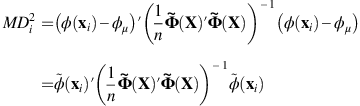
  where denotes φ(x _i )−φ _μ .Then,

  

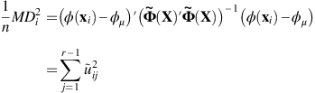
  where r−1 is the number of eigenvalues of and is an ith element of jth eigenvector of , which is sorted in descending order of eigenvalue size.

• ii) The unit length-scaled distance SD _i to the mean vector in a transformed space by KPCA can be written as since λ _i is a variance of the ith kernel principal component and is the projection of the ith observation onto the direction v _j (ie, jth kernel principal component). Owing to the following relationship between u _i and v _i ,

SD _i can be rewritten as Therefore,

Appendix C

Proof of Proposition 2

If r=n, As U is an orthogonal matrix, for all i.

Appendix D

Proof of Proposition 3

It can be proven in a similar approach as that adopted in Appendix A by the SVD. By the spectral decomposition, K can be decomposed as K=UDU′, where U is an n × n matrix whose columns are eigenvectors of K, and D is an n × n diagonal matrix with eigenvalues λ _i for i=1, …, n of K. We assume that λ _i is the ith largest eigenvalue and eigenvectors are sorted in the descending order of eigenvalues. An inverse of K+γI _n can then be written as

Equation (6) can be rewritten as

Therefore, the hat diagonal element of is given by

where r is the number of eigenvalues of K, λ _j is a jth largest eigenvalue of K, and u _ij is an ith element of jth eigenvector of K.

We can verify that (i) and (ii) of Proposition 3 can be derived using the above results. If we assume Φ(X) is centred, can be described by kernel PCA (see the proof of Proposition 1). Since can be rewritten as

Therefore, the leverage of an observation that lies in the direction of major principal component (in the feature space) becomes smaller than the leverage of an observation that lies in the direction of minor principal component (in the feature space).

Appendix E

Derivation of Equation (6)

For any matrix U and V, where I+UV and I+VU are nonsingular, the following matrix identity property holds,

Letting U=(1)/(γ)Φ(X)′ and V=Φ(X), Equation (5) can be rewritten as,

Let K=[K _ij ]_i,j=1ⁿ be an n × n matrix with entries K _ij =k(x _i , x _j )=φ(x _i )′φ(x _j ) for i, j=1, …, n. Then Equation (5) can be rewritten as the following equation.

Appendix F

Derivation of the estimates of training response values in Section 3.4

From Equation (10), the following results can be obtained.

where

Then, in the above equation can be rewritten by using the matrix identity property. Letting U=(1)/(λ)Φ(X)′ and V=QΦ(X), β is given by

Thus,

References

Askin RG and Montgomery DC (1980). Augmented robust estimators. Technometrics 22 (3): 333–341.
Beaton AE and Tukey JW (1974). The fitting of power series, meaning polynomials, illustrated on band-spectroscopic data. Technometrics 16 (2): 147–185.
Billor N and Kiral G (2008). A comparison of multiple outlier detection methods for regression data. Communications in Statistics—Simulation and Computation 37 (3): 521–545.
Bishop CM (2006). Pattern Recognition and Machine Learning. Springer: New York.
Brabanter K et al (2009). Robustness of kernel based regression: A comparison of iterative weighting schemes. In: Proceedings of the 19th International Conference on Artificial Neural Networks: Part I, Springer Berlin Heidelberg: Limassol, Cyprus, pp 100–110.
Buxton LHD (1920). The anthropology of Cyprus. The Journal of the Royal Anthropological Institute of Great Britain and Ireland 50: 183–235.
Christmann A and Steinwart I (2007). Consistency and robustness of kernel-based regression in convex risk minimization. Bernoulli 13 (3): 799–819.
Coakley CW and Hettmansperger TP (1993). A bounded influence, high breakdown, efficient regression estimator. Journal of the American Statistical Association 88 (423): 872–880.
Debruyne M, Christmann A, Hubert M and Suykens JaK (2010). Robustness of reweighted least squares kernel based regression. Journal of Multivariate Analysis 101 (2): 447–463.
Dufrenois F, Colliez J and Hamad D (2009). Bounded influence support vector regression for robust single-model estimation. IEEE Transactions on Neural Networks 20 (11): 1689–1706.
Fang Y and Jeong MK (2008). Robust probabilistic multivariate calibration model. Technometrics 50 (3): 305–316.
Handshin E, Schweppe FC, Kohlas J and Fiechter A (1975). Bad data analysis for power system state estimation. IEEE Transactions on Power Apparatus and Systems 94 (2): 329–337.
Hawkins DM, Bradu D and Kass GV (1984). Location of several outliers in multiple-regression data using elemental sets. Technometrics 26 (3): 197–208.
Holland PW (1973). Weighted ridge regression: Combining ridge and robust regression methods. NBER Working Paper: Cambridge, MA.
Jianke Z, Hoi S and Lyu MRT (2008). Robust regularized kernel regression. IEEE Transactions on Systems, Man, and Cybernetics, Part B: Cybernetics 38 (6): 1639–1644.
Kimeldorf GS and Wahba G (1970). A correspondence between Bayesian estimation on stochastic processes and smoothing by splines. The Annals of Mathematical Statistics 41 (2): 495–502.
Krasker WS and Welsch RE (1982). Efficient bounded-influence regression estimation. Journal of the American Statistical Association 77 (379): 595–604.
Markatou M and Hettmansperger TP (1990). Robust bounded-influence tests in linear models. Journal of the American Statistical Association 85 (409): 187–190.
Micchelli CA (1986). Algebraic aspects of interpolation. Proceedings of Symposia in Applied Mathematics 36: 81–102.
Pekalska E and Haasdonk B (2009). Kernel discriminant analysis for positive definite and indefinite kernels. IEEE Transactions on Pattern Analysis and Machine Intelligence 31 (6): 1017–1031.
Peng X and Wang Y (2009). A normal least squares support vector machine (NLS-SVM) and its learning algorithm. Neurocomputing 72 (16–18): 3734–3741.
Scholkopf B and Smola A (2002). Learning with Kernels: Support Vector Machines, Regularization, Optimization, and Beyond. MIT Press: Cambridge, MA.
Simpson DG and Chang Y.-C. I. (1997). Reweighting approximate GM estimators: Asymptotics and residual-based graphics. Journal of Statistical Planning and Inference 57 (2): 273–293.
Simpson JR and Montgomery DC (1996). A biased-robust regression technique for the combined outlier-multicollinearity problem. Journal of Statistical Computation and Simulation 56 (1): 1–22.
Smits GF and Jordaan EM (2002). Improved SVM Regression Using Mixtures of Kernels. In: Proceedings of the 2002 International Joint Conference on Neural Networks, Honolulu, HI, pp. 2785–2790.
Steece BM (1986). Regressor space outliers in ridge regression. Communications in Statistics: Theory and Methods 15 (12): 3599–3605.
Suykens JaK, De Brabanter J, Lukas L and Vandewalle J (2002a). Weighted least squares support vector machines: Robustness and sparse approximation. Neurocomputing 48 (1–4): 85–105.
Suykens JaK, Van Gestel T, De Brabanter J, De Moor B and Vandewalle J (2002b). Least Squares Support Vector Machines. World Scientific Publishing: Singapore.
Vapnik VN (2000). The Nature of Statistical Learning Theory. Springer Verlag: New York.
Walker E and Birch JB (1988). Influence measures in ridge regression. Technometrics 30 (2): 221–227.
Welsch RE (1980). Regression sensitivity analysis and bounded-influence estimation. In: Kmenta J and Ramsey JB (eds). Evaluation of Econometric Models. Academic Press: New York.
Wen W, Hao Z and Yang X (2008). A heuristic weight-setting strategy and iteratively updating algorithm for weighted least-squares support vector regression. Neurocomputing 71 (16–18): 3096–3103.
Zhao YP and Sun JG (2008). Robust support vector regression in the primal. Neural Networks 21 (10): 1548–1555.
Author information
Authors and Affiliations
Corresponding author