Rapid multi-criterial design of microwave components with robustness analysis by means of knowledge-based surrogates

Abstract

Manufacturing tolerances and uncertainties concerning material parameters, e.g., operating conditions or substrate permittivity are detrimental to characteristics of microwave components. The knowledge of relations between acceptable parameter deviations (not leading to violation of design specifications) and the nominal performance (not considering uncertainties), and is therefore indispensable. This paper proposes a multi-objective optimization technique of microwave components with tolerance analysis. The goal is to identify a set of trade-off designs: nominal performance versus robustness (quantified by the maximum input tolerance values that allow for achieving 100-percent fabrication yield). Our approach exploits knowledge-driven regression predictors rendered using characteristic points (features) of the component’s response for a rapid evaluation of statistical performance figures, along with trust-region algorithm to enable low execution cost as well as convergence. The proposed methodology is verified with the use of three microstrip circuits, a broadband filter, and two branch-line couplers (a single- and a dual-band one). It is demonstrated that a Pareto set w.r.t. nominal performance and robustness objectives can be produced using only 40 to 60 EM simulations of the respective structure (per design). Reliability of the proposed algorithm is corroborated with the use of EM-based Monte Carlo simulation.

Introduction

Inherently imperfect manufacturing procedures are the primary sources of uncertainties for microwave designs, including planar and multi-layer structures as well as waveguide components. Deviations of circuit dimensions from the nominal values may cause a potential violation of performance specifications. The latter are becoming continuously stringent, either due to demands implied by emerging application areas (5G communications¹, internet of things², wearable/implantable devices³), functionality requirements (wideband⁴, multi-band operation⁵, reconfigurability⁶), or miniaturization trends⁷. Their fulfilment is challenging even without accounting for tolerances, therefore, only a little margin is normally available to accommodate both statistical deviations and other types of uncertainties, including incomplete knowledge of material parameters, or changing environmental conditions such as temperature, mechanical deformations, etc. Needless to say, the capability of accurate assessment of the tolerance effects is of fundamental importance for ensuring design robustness. It should also be emphasized that improving the nominal performance (e.g., minimization of in-band return loss, maximization of bandwidth, etc.) generally leads to different parameter setups than those corresponding to the most robust designs^8,9. Consequently, designs of the highest practical utility are frequently sub-optimal with respect to nominal performance figures while ensuring broad enough safety margins for accommodating the tolerances.

Having the circuit topology established, the improvement of the (nominal) performance of passive microwave components is accomplished by appropriate adjustment of geometry parameters. For best results, both in terms of concurrent adjustment of system variables but also handling multiple objectives and constraints, parameter tuning should be realized using numerical optimization techniques^10,11,12. For reliability, the computational model of choice is usually based on full-wave electromagnetic (EM) analysis. As the optimization process requires repetitive simulations of the circuit at hand, the associated computational expenses may be high even for local (e.g., gradient-based) algorithms¹³, let alone global search procedures^14,15. The latter are typically nature-inspired population-based methods^16,17,18,19, the cost of which is measured in thousands of circuit analyses. Incorporating the effects of fabrication tolerances into the design process, in particular, when seeking performance-robustness trade-offs, makes the design task a multi-objective one²⁰. In computational terms, multi-objective optimization (MO) poses a more challenging task than single-objective design, and direct EM-driven MO is prohibitively expensive in most practical situations. A common workaround is surrogate-assisted optimization^21,22. The metamodels, often constructed in an iterative manner during the optimization run²³, are utilized as fast predictors, with EM analysis employed for verification purposes and model refinement²⁴. The modelling techniques popular in this context include approximation ones (kriging²⁵, Gaussian process regression, GPR²⁶, support-vector machines²⁷, neural networks²⁸, performance-driven surrogates^29,30) as well as physics-based methods (space mapping³¹, Pareto-ranking-based bisection³², sequential domain patching, SDP³³).

Evaluating the robustness of microwave designs with respect to fabrication tolerances requires statistical analysis³⁴. Quantification of uncertainties involves a definition of a suitable statistical figure of merit, which for microwave components is often the yield³⁵. The reason is that design specifications are typically formulated in a minimax sense³⁶. Consequently, robust design procedures would aim at yield maximization^37,38, which is equivalent to improving the probability of having the design requirements fulfilled with the assumed input tolerance levels. These levels are expressed as probability distributions pertinent to the manufacturing process but also possible correlations between the system variables. Robust design problem can also be formulated in terms of finding the maximum parameter deviations for which the design specifications are still satisfied (e.g., design for maximum input tolerance hypervolume, MITH³⁹). Regardless of the problem statement, uncertainty quantification (UQ) is CPU intensive when executed with the use of traditional methods such as EM-based Monte Carlo (MC) analysis. Practical UQ procedures largely incorporate surrogate modeling techniques^40,41,42. Among these, polynomial chaos expansion (PCE)⁴³ has recently become particularly popular in high-frequency electronics^44,45,46,47 because it directly estimates statistical moments (mean, variance) of the circuit responses without the necessity of executing MC.

A limited number of frameworks for multi-objective design of high-frequency components (primarily antennas) and tolerance analysis have been reported. MO of antenna structures and arrays, in which MITH is estimated by means of machine learning methods involving GPR surrogates has been proposed in Ref.³⁹. In Ref.⁴⁸, the authors employed kriging interpolation metamodels for robust multi-objective design of high-frequency components with worst-case analysis carried out based on trade-off designs generated by nature-inspired algorithms (here, PSO⁴⁹). Explicit handling of input tolerance hypervolume has been presented in⁵⁰, with the use of non-dominated sorting genetic algorithm (NSGA-II)⁵¹. The optimization process has been accelerated by means of an ensemble of competing surrogates (polynomial regression, GPR, kriging).

The subject of this work is a novel algorithmic approach to multi-criterial optimization of passive microwave circuits with explicit robustness improvement. Our methodology handles the tolerance-related figure of merit as one of the design objectives. Here, we define it as the maximum value of design variables’ deviations which ensures design specification fulfilment, i.e., yield equal to 100-percent. The second objective is related to the nominal performance of the circuit (e.g., in-band return loss level for filtering structures, power split ratio for the operating frequency for coupling circuits, etc.). Uncertainty quantification is realized using (linear) knowledge-based predictors established using characteristic points (response features) derived from EM-simulated circuit characteristics. Identification of the Pareto-optimal design with regard to the robustness- and performance-related goals is carried out sequentially, by local adjustment of the circuit dimensions for several target values of (nominal) figures of merit. Our procedure is demonstrated using a broadband bandpass filter and two equal-split branch-line couplers. In all cases, the average computational overhead of the MO process is around fifty EM simulations per trade-off design. Reliability of the procedure is corroborated using EM-based Monte Carlo simulation at chosen Pareto-optimal points. The original components of our approach encompass: (1) the development of a multi-criterial design framework with explicit handling of the circuit robustness, (2) the employment of fast response feature predictors, constructed using the knowledge of the system under design, enabling rapid and accurate uncertainty quantification, (3) demonstration of the procedure efficacy when solving real-world tolerance-aware MO tasks in multi-dimensional parameter spaces. The presented methodology can be applied for cost-efficient generation of alternative designs constituting achievable trade-offs between robustness and nominal figures of merit, facilitate decision making processes (e.g., concerning a selection of the manufacturing procedure), as well as meaningful comparison of different circuit topologies from the point of view of their immunity to fabrication tolerances.

Multi-criterial tuning of microwave circuits with explicit robustness handling

This section introduces the proposed framework for multi-criterial tuning of microwave circuits with explicit handling of fabrication tolerances. We aim at identifying a set of designs ensuring trade-off between robustness versus nominal performance of the circuit. Towards this end, “MO with tolerance analysis: Problem formulation” 1 provides a rigorous formulation of the design task. The details of uncertainty quantification procedure involving knowledge-based response feature predictors are given in “Uncertainty quantification procedure”. “Generating Pareto front” discusses iterative generation of the trade-off points, whereas “Multi-criterial optimization procedure” epitomizes the operation of the overall optimization framework.

MO with tolerance analysis: problem formulation

We start by introducing the necessary notation. Let x = [x₁ … x_n]^T stand for a vector of independent (adjustable) parameters of the circuit under design. We assume that the circuit response is simulated using full-wave EM analysis. Typically, we are interested in S-parameters versus frequency, which will be represented by S_ij(x,f) (e.g., i = j = 1 for reflection characteristic at Port 1, etc.), where f stands for frequency.

Performance-related objective

Here, multi-objective design is carried out according to two objectives, the performance- and robustness-related ones. A merit function quantifying the nominal performance of a circuit, that is, without parameter deviations arising from fabrication tolerances (or, in general, different types of uncertainties), will be denoted as F_p(x). We start by presenting two examples.

Example 1: bandpass filter

Let us describe a simplified setup (for the sake of clarity) with the only specifications pertaining to the reflection characteristics. Denoting by f_L and f_R the frequencies delimiting the target bandwidth, and S_max the maximal permitted in-band reflection value, the condition for satisfying the specs at the vector x can be defined as

$$\max \left\{ {f \in \left[ {f_{L} ,f_{R} } \right]\;:\;|S_{11} ({\varvec{x}},f)|} \right\} \le S_{\max }$$

(1)

Observe that additional requirements may be imposed in practice, simultaneously on the reflection and transmission characteristics (e.g., the highest level of in-band ripple⁵², maximum out-of-band transmission, etc.).

Example 2: multi-band coupler

Let f_R.k and f_L.k be the upper and lower frequencies determining the kth bandwidth, k = 1, …, N, and D_k be the maximal power split error at the f_0.k = 0.5[f_R.k + f_L.k]. Further, let S_k denote the intended power split ratio at f_0.k. The conditions for satisfying the specs at the design x are

$$\max \left\{ {f \in \bigcup\nolimits_{k = 1}^{N} {\left[ {f_{L.k} ,f_{R.k} } \right]} \;:\;|S_{11} ({\varvec{x}},f)|} \right\} \le S_{\max }$$

(2)

$$\max \left\{ {f \in \bigcup\nolimits_{k = 1}^{N} {\left[ {f_{L.k} ,f_{R.k} } \right]} \;:\;|S_{41} ({\varvec{x}},f)|} \right\} \le S_{\max }$$

(3)

and

$$\left| {|S_{31} ({\varvec{{x}}},f_{0.k} )| - |S_{21} ({\varvec{x}},f_{0.k} )| - S_{k} } \right| \le D_{k} \;\;\;\;\;k = 1,...,N$$

(4)

The maximum matching/isolation level S_max is typically set between − 15 and − 20 dB. Having the conditions (2)–(4) satisfied ensures that the circuit exhibits the target operating band (at the level equal to S_max) and, for all operating frequencies, provides the assumed power split (with the required tolerance D_k).

Microwave design optimization tasks are frequently formulated in a minimax sense, so that conditions such as (1) or (2)–(4) determine the minimum requirements, whereas the optimization process aims at reducing the levels of relevant responses beyond S_max. For the bandpass filter example considered above, the best nominal design x^p can be yielded by solving

$${\varvec{x}}^{p} = \arg \mathop {\min }\limits_{{\varvec{x}}} \left\{ {\max \left\{ {f \in \left[ {f_{L} ,f_{R} } \right]\;:\;|S_{11} ({\varvec{x}},f)|} \right\}} \right\}$$

(5)

For a coupler structure, improving the circuit matching |S₁₁| and isolation |S₄₁| (within the assumed operating bandwidths), and maintaining the assumed power split would lead to

$${\varvec{x}}^{p} = \arg \mathop {\min }\limits_{{\varvec{x}}} \left\{ {\max \left\{ {f \in \bigcup\nolimits_{k = 1}^{N} {\left[ {f_{L.k} ,f_{R.k} } \right]} \;:\;\max \{ |S_{11} ({\varvec{x}},f)|,|S_{41} ({\varvec{x}},f)|\} } \right\}} \right\}$$

(6)

subject to

$$|S_{31} ({\varvec{x}},f_{0.k} )| - |S_{21} ({\varvec{x}},f_{0.k} )| = S_{k} \;\;\;\;\;\;\;k = 1,...,N$$

(7)

Constraint handling, when solving (6), is usually implicit (using a penalty function approach⁵³) because evaluation of (7) is computationally expensive, i.e., requires EM analysis of the circuit.

In either case (here, a filter or a coupler), the nominal performance objective F_p(x) of our multi-criterial problem will be simply equal to S_max. It should also be mentioned that the performance objective F_p may encapsulate several design goals by itself, e.g., requirements concerning operating bandwidth and power split for the coupler structure considered before. These goals are aggregated to form a single scalar function. Such an approach is convenient because it allows for incorporating the designer’s priorities concerning the objectives. Notwithstanding, a generalized approach is also possible where specific performance-related goals are handled independently. This will be addressed elsewhere.

Robustness-related objective

We will denote by F_r(x) a scalar function used to determine the robustness of the system at hand. It is evaluated using a suitable statistical figure of merit, for example, the yield assessed for a given probability density function quantifying the fabrication inaccuracies. In this work, the metric of choice will be the maximum input tolerance levels that ensure meeting the performance specifications (cf. tolerance hypervolume³⁹). In practice, the parameter deviations are often modelled using independent normal distributions N(0,σ) (i.e., with mean equal to zero and variance σ common for all variables). If the correlations between the parameter are known (e.g., deviations of the coupled transmission line spacing are highly correlated with the deviation of the line widths), these may be represented using a covariance matrix C, leading to a generic multivariate distribution N(0,C), which can still be written as N(0,σC’), where σ is a positive scalar.

Observe that the definition F_r(x) = σ(x) emphasizes the explicit dependence of σ on circuit dimensions. The numerical procedure of evaluating F_r(x) will be discussed at length in “Uncertainty quantification procedure”.

MO with tolerance analysis: problem formulation

Having defined the performance- (“Performance-related objective”) and robustness-related objectives (“Robustness-related objective”), we are in a position to formulate the robust multi-criterial design problem as

$${\varvec{x}}^{*} = \arg \mathop {\min }\limits_{{\varvec{x}}} \left[ {F_{p} ({\varvec{x}})\;\;\;F_{r} ({\varvec{x}})} \right]$$

(8)

The meaning of (8) is to concurrently enhance the intended nominal performance F_p(x) along with the robust-related objective F_r(x).

It is intuitively clear that the objectives F_p and F_r stay in conflict because stricter performance demands reduce the tolerance for parameter variations. Among available nominal performance versus robustness trade-offs, one can distinguish two extreme situations, namely, the best nominal parameter vector x^p (cf. “Performance-related objective”), and the design x^r obtained for the maximum assumed value of F_p that is acceptable for a design task at hand. The latter can also correspond to any other target value according the existing priorities (e.g., − 15 dB maximum in-band reflection level in the case of a filter). Let us briefly characterize these two designs below:

• • Vector x^p

  This design realizes the best possible performance with respect to the specifications imposed on the circuit (for example features the minimum reflection within the frequency range of interest). At the same time, x^p exhibits the lowest possible robustness, especially, the fabrication yield is zero (for any parameter deviation probability distribution); also, the maximum input tolerance levels that ensure fulfilment of the specs are also zero. The reason is that altering x_p (e.g., by introducing random deviations) necessarily worsens F_p(x). Further, the design space subset encompassing feasible designs with regard to the performance conditions (e.g., (1) for a filter or (2)–(4) for a coupler) is of the form {x^p} (that is assuming a uniqueness of solution to (5) or (6), (7)).

• • Vector x^r

  This design is obtained for the most relaxed specification targets, therefore, it is characterized by the largest margin of performance as compared to x^p. This also means that x^r features the largest robustness as measured by F_r. In other words, placing the design in the centre of the feasible region permits to achieve maximum input tolerance levels which, in turn, permit to achieve 100-percent yield. This is because, for maximum F_p, the feasible region is of the largest volume.

  The above discussion indicates that designs x^p and x^r determining the span of the Pareto front corresponding to the problem (8) are the ‘outermost’ Pareto-optimal points. Multi-objective optimization aims at identifying a discrete group of points being globally nondominated in the Pareto sense⁵⁴ for both considered objectives, F_r and F_p. This set will be a representation of the achievable trade-offs between robustness and nominal performance. “Uncertainty quantification procedure”, “Generating Pareto front” and “Multi-criterial optimization procedure” describe the proposed approach to accomplishing this task, whereas Fig. 1 illustrates graphically the discussed concepts.

  Figure 1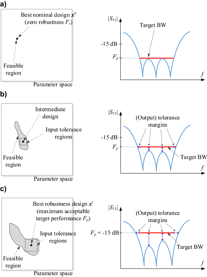

  

  Multi-criterial microwave design with robustness evaluation. Gray manifold indicates the feasible region encompassing the vectors for which, for a given F_p, the specifications are met (the feasible region is enlarged for the relaxed F_p). The right panels show reflection responses at exemplary designs of a broadband filter for various values of the assumed nominal objective F_p: (a) the highest-quality nominal design x^p; here, the feasible manifold only consists the design x^p itself, consequently, the input tolerance equals 0; (b) intermittent design: larger feasible region with the maximum robustness point residing in the centre; (c) the most robust design (for which acceptable value of F_p is the highest, for example, − 15 dB for in-band filter characteristic): the input tolerance values are maximum when centering the design. The design set rendered for various F_p constitute a Pareto set comprising the best robustness vs. performance trade-offs.

Uncertainty quantification procedure

As mentioned in “Robustness-related objective”, the measure F_r(x) of the circuit robustness is defined to be the highest value of input tolerances, parameterized by the variance σ of the probability distribution selected to describe the parameter deviations’ statistical allocation. The ‘maximum level’ is viewed as the largest value of σ enabling to obtain 100 percent fabrication yield.

Fabrication yield. Monte Carlo simulation. Robustness objective

The formal definition of yield Y at the design x is⁵⁵

$$Y({\varvec{x}}) = \int\limits_{{X_{f} }} {p({\varvec{y}},{\varvec{x}})d{\varvec{y}}}$$

(9)

with p(y, x) being a function of joint probability density that describes the point y variations with regard to the design x. The feasible space is denoted by X_f, i.e., it is the parameter region containing vectors that meet the performance specifications (such as (1) in the case of filters, or (2)–(4) for couplers, cf. “Performance-related objective”). However, the feasible space is not given explicitly, therefore direct integration of (9) is hardly possible. Instead, it is possible to approximate the yield, utilizing, e.g., Monte Carlo (MC) simulation⁵⁶. We have

$$Y({\varvec{x}}) = N_{r}^{ - 1} \sum\nolimits_{k = 1}^{{N_{r} }} {H({\varvec{x}}^{(k)} )}$$

(10)

The random observables x^(k) in (10) are of the form x^(k) = x + dx^(k), k = 1, …, N_r, where dx^(k) are rendered using the function p. Unfortunately, the MC analysis is slowly convergent (the yield estimation speed is proportional to (N_r)^−1/2), so that sizeable datasets are indispensable to provide meaningful results. Consequently, direct EM-driven MC is an expensive procedure. In practice, it is most often expedited using surrogate modeling methods^40–47.

The definition and the practical ways of estimating the yield are necessary to evaluate the robustness objective. Recall, that F_r(x) = σ(x) is the largest variance that ensures 100-percent yield. Consequently, it can be found as

$$F_{r} ({\varvec{x}}) = - \arg \mathop {\max }\limits_{\sigma } \left\{ {Y({\varvec{x}},\sigma ) = 1} \right\}$$

(11)

The notation Y(x,σ) in (11) is to emphasize that the input probability distribution variance delimits the parameter deviation values, thereby, the yield.

Response features. Design problem reformulation

For computational-efficiency, in this work, the evaluation of (11) involves knowledge-based predictors rendered using response features as described in the remaining part of this section. Response feature technology serves to expedite and enhance reliability of local optimization of antenna structures⁵⁷. It exploits a close-to-linear dependence between the frequency and level coordinates of adequately chosen characteristic attributes of the circuit responses and the system designable parameters. The feature points are chosen to carry sufficient amount of information from the point of view of whatever design task is to be undertaken, in particular, to determine satisfaction or violation of the assumed performance requirements⁵⁷. Capitalizing on problem-specific knowledge extracted from the system outputs by reformulating design problems in terms of response features brings significant advantages: faster convergence of optimization algorithms⁵⁸, enables global search capabilities even when using local methods⁵⁹, as well as allows for lowering the training data acquisition cost of setting up surrogate models⁶⁰.

As mentioned above, the feature point definition depends on design specifications (minimax, L-square, frequency-based, level-based) as well as the type of the circuit (filter, power divider, coupler, etc.). If the figure of interest is the circuit operating bandwidth, the feature points would correspond to the frequencies determining the bandwidth at the target level (e.g., − 20 dB) as well as additional points such as local maxima of the return loss characteristics within the frequency range of interest (in the case of filters). Possible allocation of the feature points for two exemplary microwave circuits: a bandpass filter and a coupler can be found in Fig. 2.

Figure 2

Exemplary features points: (a) S-parameters of a bandpass filter, characteristic points refer to − 15 dB level of return loss characteristic along with its local in-band maxima; the features allow for assessing if |S₁₁| meets the matching conditions within the following band: 5.9 GHz to 10.6 GHz; (b) coupler’s S-parameters and the features referring to − 20 dB level of |S₁₁| and |S₄₁| characteristics (o), as well as |S₂₁| and |S₃₁| at the intended operational frequency 1.5 GHz (◻); the features permit to assess meeting the design requirements within the 100 MHz bandwidth around 1.5 GHz, and maximum power split error equal to 0.5 dB at this frequency. Designs fulfilling and infringing the specs are shown in the left- and right-hand-side panels, respectively.

Handling response features through numerical procedures requires their rigorous description. Let P(x) be a (feature) vector containing the relevant information about the feature points pertinent to a given design task at the vector x. We have

$${\varvec{P}}({\varvec{x}}) = [p_{1} ({\varvec{x}})\;p_{2} ({\varvec{x}})\;...\;p_{{N_{p} }} ({\varvec{x}})]^{T}$$

(12)

in which p_k(x) are the coordinates of the feature points (either levels or frequencies). The feature point data is derived from the EM-simulated circuit outputs.

In order to clarify the matter further, let us consider two examples. The first example is a Nth-order bandpass filter whose design specs are given by (1) (“Performance-related objective”); here, the vector P has the following form

$${\varvec{P}}({\varvec{x}}) = [p_{1} ({\varvec{x}})\;p_{2} ({\varvec{x}})\;...\;p_{N + 1} ({\varvec{x}})]^{T} = [f_{1} ({\varvec{x}})\;f_{2} ({\varvec{x}})\;l_{1} ({\varvec{x}})\;\;...\;\;l_{N - 1} ({\varvec{x}})]^{T}$$

(13)

Note that the first two entries are frequencies f₁ and f₂ corresponding to S_max (such as minus 20 dB) level of |S₁₁|; the remaining entries l_k refer to in-band maxima of |S₁₁| (specifically, their reflection levels). The performance requirements (1) may be rewritten in terms of the feature vector as

$$f_{1} ({\varvec{x}}) \le f_{L} ,\;\;\;f_{2} ({\varvec{x}}) \ge f_{R}$$

(14)

$$l_{k} ({\varvec{x}}) \le S_{\max } ,\;k = 1, \ldots ,N{-}{1}$$

(15)

Clearly, the filter has to be well tuned to ensure the presence of all maxima; however, this condition holds at the nominal design. In some cases, during optimization run, the number of in-band maxima may be different form that at the nominal design. Nevertheless, such a situation does not occur for the considered parameter variations. In practice, variations being so large that it would affect the shapes of the filter characteristics (and thereby the number of in-band maxima) are unlikely to happen, as this would mean, e.g., error of etching the geometrical details of the filter of large fractions of millimeter (i.e., comparable to their width). The actual manufacturing procedures (chemical etching or mechanical milling) are considerably more accurate with the deviations corresponding to the levels considered in the paper.

Another example is a microwave coupler. If design specifications follow (2)–(4), the feature points should correspond to S_max (e.g., − 20 dB) levels of |S₁₁| and |S₄₁|, but also the values of |S₂₁| and |S₃₁| (i.e., coupler’s transmission responses) at the target operating frequency. Therefore, the feature vector is as follows

$${\varvec{P}}({\varvec{x}}) = [p_{1} ({\varvec{x}})\;p_{2} ({\varvec{x}})\;...\;p_{6} ({\varvec{x}})]^{T} = [f_{1} ({\varvec{x}})\;f_{2} ({\varvec{x}})\;f_{3} ({\varvec{x}})\;f_{4} ({\varvec{x}})\;l_{1} ({\varvec{x}})\;l_{2} ({\varvec{x}})]^{T}$$

(17)

Here, the frequencies of the S_max level of |S₁₁| are denoted as f₁ and f₂, whereas the frequencies corresponding to the S_max level of |S₄₁| are referred to as f₃ and f₄. Moreover, l₁ and l₂ are the levels of |S₂₁| and |S₃₁| at the coupler’s intended operational frequency, respectively (cf. Figure 2b). This concept can be generalized for a multi-band coupler:

$$\begin{gathered} {\varvec{P}}({\varvec{x}}) = [p_{1} ({\varvec{x}})\;p_{2} ({\varvec{x}})\;...\;p_{6N} ({\varvec{x}})]^{T} = \\ [f_{1.1} ({\varvec{x}})\;f_{2.1} ({\varvec{x}})\;f_{3.1} ({\varvec{x}})\;f_{4.1} ({\varvec{x}})\;l_{1.1} ({\varvec{x}})\;l_{2.1} ({\varvec{x}})\;\;...\;\;f_{1.N} ({\varvec{x}})\;f_{2.N} ({\varvec{x}})\;f_{3.N} ({\varvec{x}})\;f_{4.N} ({\varvec{x}})\;l_{1.N} ({\varvec{x}})\;l_{2.N} ({\varvec{x}})]^{T} \\ \end{gathered}$$

(18)

where the operating band (from 1 to N) is indicated by the second subscript.

The design requirements (2)–(4) expressed in terms of the feature points will become

$$f_{1.k} ({\varvec{x}}) \le f_{L.k} ,\;\;\;f_{3.k} ({\varvec{x}}) \le f_{L.k} ,\;k = {1}, \ldots ,N$$

(19)

$$f_{2.k} ({\varvec{x}}) \ge f_{R.k} ,\;\;\;f_{4.k} ({\varvec{x}}) \ge f_{R.k} ,\;k = {1}, \ldots ,N$$

(20)

$$|l_{1.k} ({\varvec{x}}) - l_{2.k} ({\varvec{x}})| \le D_{k} ,\;k = {1}, \ldots ,N$$

(21)

Knowledge-based predictors

The fundamental benefits of incorporating response feature technology into the uncertainty quantification process is the abovementioned weakly nonlinear (in many cases, close to linear) dependence of the vector P entries on the circuit dimensions. Consequently, even simple (in particular, linear) metamodels may exhibit predictive power sufficient for reliable statistical analysis in a vicinity of the nominal design. Moreover, the computational cost of setting up such knowledge-based models is considerably lower than for surrogates representing the entire frequency characteristics of the circuit of interest.

Consider a feature-based predictor L_P⁽ⁱ⁾(x) constructed at the point x⁽ⁱ⁾, and representing the vector of response features P(x) in the neighborhood of x⁽ⁱ⁾

$$L_{P}^{(i)} ({\varvec{x}}) = [p_{L.1} ({\varvec{x}})\;...\;p_{{L.N_{p} }} ({\varvec{x}})]^{T} = \left[ \begin{gathered} l_{0.1} + {\varvec{L}}_{1}^{T} ({\varvec{x}} - {\varvec{x}}^{(i)} ) \\ \vdots \\ l_{{0.N_{p} }} + {\varvec{L}}_{{2N_{p} }}^{T} ({\varvec{x}} - {\varvec{x}}^{(i)} ) \\ \end{gathered} \right]$$

(22)

Solving linear regression problems L_P⁽ⁱ⁾(x_B^(j)) = P(x_B^(j)) allows for identifying the predictor model, with x_B^(j), j = 1, …, n + 1, being trial points, and P(x_B^(j)) yielded from EM-simulated circuit response. We have

$$\left[ \begin{gathered} l_{0.j} \\ {\varvec{L}}_{j} \\ \end{gathered} \right] = \left[ \begin{gathered} 1\;\;({\varvec{x}}_{B}^{(1)} - {\varvec{x}}^{(i)} )^{T} \\ \vdots \\ 1\;\;({\varvec{x}}_{B}^{(n + 1)} - {\varvec{x}}^{(i)} )^{T} \\ \end{gathered} \right]^{ - 1} \left[ \begin{gathered} p_{j} ({\varvec{x}}_{B}^{(1)} ) \\ \vdots \\ p_{j} ({\varvec{x}}_{B}^{(n + 1)} ) \\ \end{gathered} \right],\;j = {1}, \ldots ,N_{p}$$

(23)

Here, the training vectors are allocated by perturbing the center point x_B⁽¹⁾ = x⁽ⁱ⁾ as x_B^(j) = x⁽ⁱ⁾ + [0 … 0 d 0 … 0]^T, i.e., the (j−1)th entry equals d. We use the value d = 3σ, i.e., the perturbations are equal to the largest deviations of the parameters.

Robustness objective evaluation

Evaluation of the robustness-related objective function (11) requires repetitive computation of the yield, which is realized here by numerically integrating the probability density function p in (9). In order to expedite the process, we utilize the feature-based predictor L_P⁽ⁱ⁾(x), which allows for a fast assessment of design specifications (e.g., conditions (14), (15) for the exemplary filter, or (18)–(20) for the coupler). Estimation of the yield Y(x,σ) is carried out with the use of a large number of random observables x_r^(j) (in our experiments, we have 100,000 points) rendered following the probability distribution parameterized by the variance σ. The routine operates in the following manner:

• 1. For a variance σ, render the set of random observations {x_r^(j)}_{j = 1, …, Nr};

• 2. For each j = 1, …, N_r, evaluate the feature-based predictor L_P⁽ⁱ⁾(x_r^(j));

• 3. For all x_r^(j), j = 1, …, N_r, verify design specification conditions (e.g., (14), (15), or (18)–(20) using predicted feature coordinates p_L.k(x_r^(j));

• 4. Calculate estimated yield Y(x,σ) as in (10).

Observe that for large N_r the standard deviation of the Monte Carlo process outcome may be greatly reduced. All operations (in particular, Steps 2 and 3) are vectorized to further reduce the CPU cost of yield evaluation.

Having a procedure for fast yield evaluation, the robustness objective F_r is computed by solving (11). Here, as Y is dependent on a scalar parameter σ, we use a golden ratio search⁶¹. In general, e.g., joint Gaussian distribution described by a covariance matrix, generic gradient-based procedures may be applied.

Generating Pareto front

The goal of the proposed multi-criterial optimization with robustness evaluation is to render a discrete sequence of designs being the best attainable robustness versus performance trade-offs. As discussed in “MO with tolerance analysis: Problem formulation”, the Pareto front span is defined by the vector x^p (the best nominal design, “Performance-related objective”, cf. (5) and (6), (7)), and the vector x^r, representing the best robust design (i.e., that of the maximum acceptable target level S_max).

We aim at generating N_P trade-off designs, starting from x⁽¹⁾ = x^p. Let S_max.1 denote the value of the function F_p at design x^p. For the filter example considered before (cf. (1)), it is

$$S_{\max .1} = \max \left\{ {f \in \left[ {f_{L} ,f_{R} } \right]\;:\;|S_{11} ({\varvec{x}}^{p} ,f)|} \right\}$$

(24)

For the microwave coupler (cf. (2)–(4)), we have

$$S_{\max .1} = \max \left\{ {f \in \bigcup\nolimits_{k = 1}^{N} {\left[ {f_{L.k} ,f_{R.k} } \right]} \;:\max \{ \;|S_{11} ({\varvec{x}}^{p} ,f)|,|S_{41} ({\varvec{x}}^{p} ,f)|\} } \right\}$$

(25)

Let us denote as S_max.NP the maximum acceptable level of target S_max. The points x^(j), j = 2, …, N_P, i.e., trade-off solutions, are to be rendered for the assumed values S_max.j, j = 2, …, N_P, distributed in equal intervals between S_max.1 and S_max.NP (recall, that F_p(x^(j)) = S_max.j)

$$F_{p} ({\varvec{x}}^{(j)} ) = S_{\max .j} = S_{\max .1} + \left[ {S_{{\max .N_{P} }} - S_{\max .1} } \right]\frac{j - 1}{{N_{P} - 1}}$$

(26)

Having defined S_max.j, the trade-off design x^(j) is found as

$${\varvec{x}}^{(j)} = \arg \mathop {\min }\limits_{{\varvec{x}}} F_{r} ({\varvec{x}})$$

(27)

with S_max set to S_max.j in the relevant objective function, cf. (1) for the filter, and (2)–(4) for the coupler, as well as their response feature counterparts (14), (15), and (18)–(20). In plain words, in order to find x^(j), the circuit at hand is optimized to improve its robustness as defined by (11), assuming that the target level S_max = S_max.j.

The solution to problem (26) is found iteratively, incorporating the trust-region (TR) principles⁶². More specifically, the design x^(j) is approximated by a sequence of vectors x^(j.i+1) produced as

$${\varvec{x}}^{(j.i + 1)} = \arg \mathop {\min }\limits_{{||{\varvec{x}} - {\varvec{x}}^{(j.i)} || \le d^{(i)} }} F_{r} ({\varvec{x}})$$

(28)

The first of these approximations (i.e., the starting point for the iterative procedure (27)) is the previously obtained trade-off design; we have x^(j.0) = x^(j−1). The function F_r (i.e., robustness objective) is evaluated as described in “Robustness objective evaluation”. The solution to (27) is identified in the neighborhood of the current point, given by ||x − x^(j.i)||≤ d⁽ⁱ⁾, where positive scalar d⁽ⁱ⁾ constitutes the trust region size parameter; it is re-adjusted upon each consecutive iteration in compliance with the standard TR rules⁶². A decision about accepting or rejecting the new approximate solution x^(j.i+1) is based upon the gain ratio

$$r = \frac{{F_{r}^{\# } ({\varvec{x}}^{(j.i + 1)} ) - F_{r} ({\varvec{x}}^{(j.i)} )}}{{F_{r} ({\varvec{x}}^{(j.i + 1)} ) - F_{r} ({\varvec{x}}^{(j.i)} )}}$$

(29)

The denominator thereof quantifies enhancement of the robustness according to the feature-based predictor. The numerator accounts for the actual improvement, although it is still approximated by using an auxiliary function F_r^#, calculated as in “Robustness objective evaluation”, still the model L_P^(j.i) is substituted by L_P^#(j.i), which is built as in (21), (22) yet, instead of the vector [l_0.1 … l_0.2N]^T, the feature vector P(x^(j.i+1)) derived from EM-simulated response of the circuit at hand at x^(j.i+1) is utilized. Note that using F_r^# instead of a fully updated surrogate L_P^(j.i+1) brings tremendous computational advantages because its evaluation only requires one EM analysis. Nevertheless, the assessment made with the use of (28) is generally reliable because the gradients of the features do not change abruptly between subsequent iteration points x^(j.i) and x^(j.i+1). The reason is small design relocation (comparable to σ) but also weakly nonlinear relation between the coordinates of the features and circuit dimensions.

The design x^(j.i+1) is approved for positive value of the gain ratio r. For r < 0, the design is discarded and the iteration is relaunched with a smaller d⁽ⁱ⁾. On the other hand, if the r is close to one (here, r > 0.75), the size parameter d⁽ⁱ⁾ is increased before the next iteration. The algorithm is terminated if either condition is met: (i) ||x⁽ⁱ⁺¹⁾ − x⁽ⁱ⁾||< ε (convergence in argument) or (ii) d⁽ⁱ⁾ < ε (shrinking of the trust region). Here, we use ε = 10⁻³. The entire multi-criterial optimization procedure has been illustrated in Fig. 3.

Figure 3

Graphical illustration of multi-criterial design with robustness evaluation. The graph visualizes successive rendition of performance-robustness trade-off solutions, starting from the best nominal design x^p.

Multi-criterial optimization procedure

The operating flow of the proposed multi-criterial optimization algorithm with robustness evaluation has been shown in Fig. 4. The initial setup concerning performance-related design objectives, maximum acceptable performance target level S_max, etc., is up to the user. The best nominal design is usually obtained through a local search. The target performance thresholds S_max.j are determined based on S_max, the performance-related objective value F_p(x^p), as well as the required number of trade-off points N_P. These are identified using the iterative process described in “Generating Pareto front”.

Figure 4

Operating flow of the proposed multi-criterial optimization algorithm with knowledge-based robustness evaluation using feature-based predictors and trust-region-based parameter adjustment.

Verification case studies

This section demonstrates the functioning and performance of the multi-criterial optimization framework introduced in “Multi-criterial tuning of microwave circuits with explicit robustness handling”. Numerical experiments are based on three microstrip structures, a broadband bandpass filter, and two branch-line couplers, a single-band and a dual-band one. The performance-related objective F_p(x) is formulated using the highest level of reflection characteristic (filter) or matching and isolation characteristics (couplers) within the frequency range of interest. In the latter case, an additional requirement is equal power split condition at the centre frequencies of the respective circuits with 0.5 dB tolerance. The robustness-related performance figure F_r(x) is given as the maximal variance of the Gaussian distributions characterizing the deviations of the geometry parameters, ensuring the perfect (100 percent) fabrication yield. The obtained results are validated by performing EM-driven Monte Carlo simulation at the chosen trade-off solutions obtained for the considered circuits.

Case study 1: broadband bandpass filter

Consider a broadband bandpass filter with stepped-impedance resonator⁶³ presented in Fig. 5. The circuit is implemented on RO4003C substrate (ε_r = 3.55, h = 0.305 mm). The design variables are x = [L₁ L₂ L₃ W₁ W₂ W₃]^T (all in millimeters). The width of the feed line equals W₀ = 0.66 mm. The EM simulation model of the filter is evaluated using time-domain solver of CST Microwave Studio.

Figure 5

Geometry of the broadband bandpass filter with stepped-impedance resonator⁶³.

The intended filter operating bandwidth is delimited by f_L = 6.0 GHz and f_R = 10.0 GHz (cf. “Performance-related objective”). The best nominal design x^p = [4.40 5.61 3.76 6.55 1.01 0.48]^T has been obtained by solving the design task (5), i.e., by minimizing the maximum in-band reflection level |S₁₁| within the frequency range from f_L = 6 to f_R = 10 GHz. The problem (5) has been solved using the trust-region algorithm, and the achieved maximum in-band reflection is around − 22 dB. At this design, the robustness-related merit function F_r(x^p) is zero (cf. “MO with tolerance analysis: Problem formulation”). In the course of multi-criterial design, several supplementary trade-off solutions (namely six) have been produced, for S_max.2 = − 20 dB, S_max.3 = − 19 dB, up to S_max.7 = − 15 dB (the highest tolerable value of the reflection). Table 1 provides the relevant data with respect to the trade-off solutions, and Fig. 6 presents the obtained Pareto set. Finally, in Fig. 7, EM-based Monte Carlo (MC) analysis is visualized for some designs of Table 1. MC simulation has been executed for the sake of validation of robustness predictions produced by the feature-based surrogates. More specifically, we need to verify the agreement between the yield maintained during the optimization process (which is supposed to be 100 percent), and its estimation obtained at the level of EM analysis. As it turns out, the MC-based yield is between 99 and 100 percent for all designs x⁽²⁾ through x⁽⁷⁾. At the same time, it should be noted that—due to its high CPU cost—MC was run with only 500 samples, so, the standard deviation of yield estimation is increased.

Table 1 Results of multi-criterial design with robustness evaluation for a bandpass filter of Fig. 5

Figure 6

Bandpass filter of Fig. 5: trade-off designs (performance vs. robustness) generated using the multi-criterial optimization procedure of “Multi-criterial tuning of microwave circuits with explicit robustness handling”. The maximal acceptable reflection level within the frequency band of interest is marked using vertical line.

Figure 7

EM-based Monte Carlo analysis of the bandpass filter of Fig. 5 at some trade-off points from Table 1. The circuit output at the selected trade-off design is marked black, whereas 500 random trial points rendered following the probability distribution of the variance σ = F_r are shown using grey color. The specs are indicated by thin lines: (a) design x⁽²⁾, (b) design x⁽⁴⁾, (c) design x⁽⁷⁾.

The proposed multi-criterial optimization procedure is cost-effective. The total cost of rendering the entire Pareto set equals 306 EM simulations of the filter circuit (with the average expenses of generating a trade-off solution corresponding to merely 44 EM analyses). As elaborated on in “Multi-criterial tuning of microwave circuits with explicit robustness handling”, this level of efficiency is mainly possible due to the involvement of the feature-based predictor models.

Case study 2: miniaturized branch-line coupler

Our second verification structure is a compact equal-split branch-line coupler (BLC)⁶⁴ presented in Fig. 8. The circuit is implemented on AD300 substrate (ε_r = 2.97, h = 0.76 mm). We have the independent designable parameters: x = [g l_1r l_a l_b w₁ w_2r w_3r w_4r w_a w_b]^T (dimensions in millimeters for absolute parameters; relative parameters indicated by subscript r are unitless). Remaining dimensions: L = 2dL + L_s, L_s = 4w₁ + 4 g + s + l_a + l_b, W = 2dL + W_s, W_s = 4w₁ + 4 g + s + 2w_a, l₁ = l_bl_1r, w₂ = w_aw_2r, w₃ = w_3rw_a, and w₄ = w_4rw_a, w_c = 1.9 mm. The circuit is simulated using transient solver of CST Microwave Studio.

Figure 8

Geometry of the miniaturized microstrip branch-line coupler (BLC)⁶⁴.

The intended frequency bandwidth is given f_L.1 = 1.45 GHz and f_R.1 = 1.55 GHz. Furthermore, BLC is to ensure equal power split with the tolerance of 0.5 dB, i.e., the following condition has to be satisfied: ||S₂₁| −|S₃₁||≤ S₁ = 0.5 dB at 1.5 GHz. The best nominal performance design x^p = [0.65 5.93 9.35 12.47 1.29 2.03 0.97 0.32 2.79 0.22]^T has been obtained by solving the design task (6) and (7) using the TR algorithm with S₁ = 0.5 dB, f_L.1 = 1.45 GHz and f_R.1 = 1.55 GHz. The nominal design refers to the maximal values of |S₁₁| and |S₄₁|, or F_p(x^p) = − 21.1 dB. For equal-split BLC, six supplementary trade-off solutions were rendered, for S_max.2 = − 20 dB, S_max.3 = − 19 dB, up to S_max.7 = − 15 dB (the highest tolerable level for matching and isolation). Observe that for relative variables, the deviations are re-evaluated to follow the required tolerances of the respective absolute variables taking into account the relationships from the circuit description.

Table 2 provides the numerical results, whereas Fig. 9 shows the Pareto front. Figure 10 presents graphical illustration of the EM-driven Monte Carlo analysis. As before, the value of MC-estimated yield nearly equals to 100 percent for all trade-off designs x^(k). This re-confirms prediction reliability of the feature-based predictors. The total cost of generating the entire Pareto set equals 422 EM simulations of the coupler (with the average expenditures of rendering the trade-off points equal around 60 EM analyses). It should be noted that there is no improvement of the robustness-related objective for F_p higher than − 16 dB, which is due to the fact that the robustness is limited from above by the power split condition (i.e., further relaxing of F_p cannot improve F_r anymore).

Table 2 Results of multi-criterial design with robustness evaluation for a compact BLC of Fig. 8

Figure 9

Compact BLC of Fig. 8: trade-off solutions generated using the introduced multi-criterial optimization framework. The maximal acceptable value of in-band |S₁₁| and |S₄₁| is marked using vertical line.

Figure 10

EM-based Monte Carlo analysis of the compact BLC of Fig. 8 at some trade-off points of Table 2. The circuit output at the selected trade-off design is marked black, whereas 500 random trial points rendered following the probability distribution of the variance σ = F_r are shown using grey color. The specs are indicated by thin lines: (a) design x⁽²⁾, (b) design x⁽⁴⁾, (c) design x⁽⁶⁾.

Case study 3: dual-band microstrip branch-line coupler

Our last verification structure is a dual-band branch-line coupler (BLC)⁶⁵ of Fig. 11. The circuit is implemented on RO4003 substrate (ε_r = 3.5, h = 0.51 mm). The independent design parameters are x = [L_s W_s l_3r w₁ w₂ w₃ w₄ w₅ w_v]^T. Absolute dimensions are expressed in mm. The parameter l_3r is relative and unitless. Further, we have: d_L = d_W = 10 mm, L = 2d_L + L_s, W = 2d_W + 2w₁ + (W_s− 2w_f), l₁ = W_s/2, l₂ = l₃2^1/2, l₃ = l_3r((L_s − w₃)/2 − w₄/2^1/2), l_v1 = l₃/3, l_v3 = L_s/2 − w₃/2 − l₃ + l_v1; w_f = 1.15 mm. The BLC is simulated using CST Microwave Studio. In the case of the relative variable, the corresponding parameter deviations are recalculated to match the tolerance of the respective absolute variable, here, l₃ (using the dependencies provided above).

Figure 11

Geometry of dual-band branch-line coupler⁶⁵.

The target operating bandwidths are given by f_L.1 = 2.35 GHz and f_R.1 = 2.45 GHz (lower band), and f_L.2 = 5.15 GHz and f_R.2 = 5.25 GHz (upper band). Furthermore, the BLC is to ensure equal power split with the tolerance of 0.5 dB, i.e., the following condition has to be satisfied: | |S₂₁| −|S₃₁| |≤ S₁ = S₂ = 0.5 dB at the operational frequencies equal to 2.4 GHz and 5.2 GHz. The best nominal performance design x^p = [25.03 0.80 0.78 1.96 1.29 0.41 0.79 0.34 0.34]^T (corresponding to the maximum reflection F_p(x^p) = − 21.5 dB) has been obtained by solving the design task (6) and (7) using the TR algorithm with S₁ = S₂ = 0.5 dB, f_L.1 = 2.35 GHz and also f_R.1 = 2.45 GHz, f_L.2 = 5.15 GHz and f_R.2 = 5.25 GHz. Similarly as for the previous example, six supplementary trade-off points have been rendered, for S_max.2 = − 20 dB, S_max.3 = − 19 dB, up to S_max.7 = − 15 dB.

Table 3 gathers numerical results, and Fig. 12 gives the Pareto set. Whereas Fig. 13 presents results of the simulation-based MC analysis. MC-evaluated yield, for all trade-off solutions, is around one hundred percent. The total cost of generating the entire Pareto set equals 341 EM simulations of the coupler, which corresponds to just 49 EM simulations of the BLC per design, which is consistent with the previous case studies. Similarly as for the second example, no improvement of the robustness-related objective can be observed beyond a certain value of F_p, here, − 17 dB. The reason is the same as for the BLC of Fig. 8: the robustness is limited by the assumed maximum tolerable power split error of 0.5 dB.

Table 3 Results of multi-criterial design with robustness evaluation for a dual-band BLC of Fig. 11.

Figure 12

Dual-band BLC of Fig. 11: trade-off designs rendered using the introduced multi-criterial optimization framework. The maximal acceptable value of in-band |S₁₁| and |S₄₁| is marked using vertical line.

Figure 13

EM-based Monte Carlo analysis of the dual-band BLC of Fig. 11 at some trade-off points of Table 3. The circuit output at the selected trade-off design is marked black, whereas 500 random trial points rendered following the probability distribution of the variance σ = F_r are shown using gray color. The specs are indicated by thin lines: (a) design x⁽²⁾, (b) design x⁽⁴⁾, (c) design x⁽⁵⁾.

Conclusion

This work introduced an algorithmic approach for multi-criterial optimization of microwave components with robustness evaluation. The aim is to render a set of alternate parameter vectors corresponding to the best attainable trade-offs (or Pareto set) in the sense of both the nominal performance of the circuit (i.e., neglecting possible uncertainties, primarily manufacturing tolerances), as well as its robustness. The robustness is understood as the highest possible input tolerance values still ensuring satisfaction of given performance specs with 100-percent likelihood. The proposed procedure capitalizes on rapid uncertainty quantification realized by means of the feature-based predictors, which are demonstrated to be instrumental in ensuring both computational efficiency of the algorithm and the reliability of yield estimation. The iterative rendition of trade-off designs utilizes the trust-region (TR) algorithm, which guarantees process convergence. Verification of the candidate solutions generated in the course of the TR process is carried out by reusing feature point sensitivities, which contributes to additional speedup, at the same time, the process reliability is not degraded. Our methodology has been demonstrated using three microstrip circuits, including a bandpass filter, and two microstrip couplers. The optimization cost varies between 40 and 60 EM analyses of the considered circuit with only slight dependence on the dimensionality of the design space. Accuracy of the feature-based predictors has been confirmed via simulation-driven Monte Carlo analysis of the selected trade-off designs. The MO procedure presented in this paper can be applied in support systems facilitating a selection of fabrication procedures, as well as fast determination of available compromise solutions between electrical performance of the circuit and its fabrication tolerance immunity. Other applications include robustness-related comparisons of various candidate circuit architectures (for a given application area), or determination of the required manufacturing process accuracy as a function of nominal performance demands. In our methodology, only the fabrication tolerances are considered (also referred to as aleatory uncertainties). Handling epistemic uncertainties, for example, the tolerances of dielectric relative permittivity being a result of an incomplete knowledge concerning material parameters, will be the subject of the future work.

References

Zhang, Y., Deng, J., Li, M., Sun, D. & Guo, L. A MIMO dielectric resonator antenna with improved isolation for 5G mm-wave applications. IEEE Ant. Wirel. Propag. Lett. 18, 747–751 (2019).
Taheri, M. M. S., Abdipour, A., Zhang, S. & Pedersen, G. F. Integrated millimeter-wave wideband end-fire 5G beam steerable array and low-frequency 4G LTE antenna in mobile terminals. IEEE Trans. Veh. Technol. 68, 4042–4046 (2019).
Manshari, S., Koziel, S. & Leifsson, L. Compact dual-polarized corrugated horn antenna for satellite communications. IEEE Trans. Antennas Propag. 68, 5122–5129 (2020).
Yang, X., Ge, L., Wang, J. & Sim, C. A differentially driven dual-polarized high-gain stacked patch antenna. IEEE Ant. Wirel. Propag. Lett. 17, 1181–1185 (2018).
Sang, L., Wu, S., Liu, G., Wang, J. & Huang, W. High-gain UWB Vivaldi antenna loaded with reconfigurable 3-D phase adjusting unit lens. IEEE Ant. Wirel. Propag. Lett. 19, 322–326 (2020).
Assimonis, S. D., Abbasi, M. A. B. & Fusco, V. Millimeter-wave multi-mode circular antenna array for uni-cast multi-cast and OAM communication. Sci. Rep. 11, 4928 (2021).
Li, S., Wang, S., An, Q., Zhao, G. & Sun, H. Cylindrical MIMO array-based near-field microwave imaging. IEEE Trans. Antennas Propag. 69, 612–617 (2021).
Wu, T., Li, R. & Tentzeris, M. M. A scalable solar antenna for autonomous integrated wireless sensor nodes. IEEE Ant. Wireless Propag. Lett. 10, 510–513 (2011).
Valanarasi, A. & Dhanasekaran, R. Optimum band ε shaped miniature implantable antennas for telemetry applications. IEEE Trans. Antennas Propag. 69, 55–63 (2021).
Yuan, X. et al. Ultra-wideband MIMO antenna system with high element-isolation for 5G smartphone application. IEEE Access 8, 56281–56289 (2020).
Cai, Z., Zhou, Y., Qi, Y., Zhuang, W. & Deng, L. A millimeter wave dual-lens antenna for IoT-based smart parking radar system. IEEE Internet Things J. 8, 418–427 (2021).
Rahman, A., Islam, M., Singh, M., Kibria, S. & Khtaruzzaman, M. Electromagnetic performances analysis of an ultra-wideband and flexible material antenna in microwave breast imaging: To implement a wearable medical bra. Sci. Rep. 6, 38906 (2016).
Afifi, A. I., Abdel-Rahman, A. B., El-Hameed, A. S. A., Allam, A. & Ahmed, S. M. Small frequency ratio multi-band dielectric resonator antenna utilizing vertical metallic strip pairs feeding structure. IEEE Access 8, 112840–112845 (2020).
Houret, T., Lizzi, L., Ferrero, F., Danchesi, C. & Boudaud, S. DTC-enabled frequency-tunable inverted-F antenna for IoT applications. IEEE Ant. Wirel. Propag. Lett. 19, 307–311 (2020).
Zhang, Y., Wang, H., Liao, D. & Fu, W. Phase-tuning metasurface for circularly polarized broadside radiation in broadband. Sci. Rep. 8, 2970 (2018).
Liang, Z., Lv, S., Li, Y., Liu, J. & Long, Y. Compact folded slot antenna and its endfire arrays with high gain and vertical polarization. IEEE Ant. Wirel. Propag. Lett. 19, 786–790 (2020).
Lalbakhsh, A., Afzal, M. U., Hayat, T., Esselle, K. P. & Mandal, K. All-metal wideband metasurface for near-field transformation of medium-to-high gain electromagnetic sources. Sci. Rep. 11, 9421 (2021).
Yang, G., Zhang, Y. & Zhang, S. Wide-band and wide-angle scanning phased array antenna for mobile communication system. IEEE Open J. Antennas Propag. 2, 203–212 (2021).
Ren, J., Hu, W., Yin, Y. & Fan, R. Compact printed MIMO antenna for UWB applications. IEEE Ant. Wirel. Propag. Lett. 13, 1517–1520 (2014).
Tao, J. & Feng, Q. Compact ultrawideband MIMO antenna with half-slot structure. IEEE Ant. Wirel. Propag. Lett. 16, 792–795 (2017).
Reddy, B. R. S. & Vakula, D. Compact zigzag-shaped-slit microstrip antenna with circular defected ground structure for wireless applications. IEEE Ant. Wirel. Propag. Lett. 14, 678–681 (2015).
Wang, Z., Li, C. & Yin, Y. A meta-surface antenna array decoupling (MAAD) design to improve the isolation performance in a MIMO system. IEEE Access 8, 61797–61805 (2020).
Roshna, T. K., Deepak, U., Sajitha, V. R., Vasudevan, K. & Mohanan, P. A compact UWB MIMO antenna with reflector to enhance isolation. IEEE Trans. Antennas Propag. 63, 1873–1877 (2015).
Liu, J., Esselle, K. P., Hay, S. G. & Zhong, S. Effects of printed UWB antenna miniaturization on pulse fidelity and pattern stability. IEEE Trans. Antennas Propag. 62, 3903–3910 (2014).
Hassan, E., Noreland, D., Augustine, R., Wadbro, E. & Berggren, M. Topology optimization of planar antennas for wideband near-field coupling. IEEE Trans. Antennas Propag. 63, 4208–4213 (2015).
Koziel, S. & Pietrenko-Dabrowska, A. Expedited optimization of antenna input characteristics with adaptive Broyden updates. Eng. Comp. 37, 851–862 (2019).
Koziel, S., Bekasiewicz, A., Couckuyt, I. & Dhaene, T. Efficient multi-objective simulation-driven antenna design using co-kriging. IEEE Trans. Antennas Propag. 62, 5900–5905 (2014).
Barmuta, P., Ferranti, F., Gibiino, G. P., Lewandowski, A. & Schreurs, D. M. M. P. Compact behavioral models of nonlinear active devices using response surface methodology. IEEE Trans. Microwave Theory Techn. 63, 56–64 (2015).
Ghorbani, F. et al. Deep neural network-based automatic metasurface design with a wide frequency range. Sci. Rep. 11, 7102 (2021).
Jacobs, J. P. & Koziel, S. Two-stage framework for efficient Gaussian process modeling of antenna input characteristics. IEEE Trans. Antennas Propag. 62, 706–713 (2014).
Polikar, R. Ensemble learning. In Ensemble Machine Learning (eds Zhang, C. & Ma, Y.) 1–34 (Springer, 2012).
Baratta, I. A., de Andrade, C. B., de Assis, R. R. & Silva, E. J. Infinitesimal dipole model using space mapping optimization for antenna placement. IEEE Ant. Wirel. Propag. Lett. 17, 17–20 (2018).
Su, Y., Li, J., Fan, Z. & Chen, R, Shaping optimization of double reflector antenna based on manifold mapping. In International Applied Computational Electromagnetics Society Symposium (ACES), 1–2 (Suzhou, China, 2017).
Koziel, S. & Unnsteinsson, S. D. Expedited design closure of antennas by means of trust-region-based adaptive response scaling. IEEE Ant. Wirel. Propag. Lett. 17, 1099–1103 (2018).
Koziel, S. & Leifsson, L. Simulation-driven design by knowledge-based response correction techniques (Springer, 2016).
Zhang, C., Feng, F., Gongal-Reddy, V., Zhang, Q. J. & Bandler, J. W. Cognition-driven formulation of space mapping for equal-ripple optimization of microwave filters. IEEE Trans. Microw. Theory Techn. 63, 2154–2165 (2015).
Tak, J., Kantemur, A., Sharma, Y. & Xin, H. A 3-D-printed W-band slotted waveguide array antenna optimized using machine learning. IEEE Ant. Wirel. Propag. Lett. 17, 2008–2012 (2018).
Liu, B., Koziel, S. & Ali, N. SADEA-II: A generalized method for efficient global optimization of antenna design. J. Comp. Design Eng. 4, 86–97 (2017).
Lim, D. K. et al. A novel surrogate-assisted multi-objective optimization algorithm for an electromagnetic machine design. IEEE Trans. Magn. 51, 8200804 (2015).
Dong, J., Qin, W. & Wang, M. Fast multi-objective optimization of multi-parameter antenna structures based on improved BPNN surrogate model. IEEE Access 7, 77692–77701 (2019).
Xiao, S. et al. Multi-objective Pareto optimization of electromagnetic devices exploiting kriging with Lipschitzian optimized expected improvement. IEEE Trans. Magn. 54, 7001704 (2018).
Koziel, S., Cheng, Q. S. & Li, S. Optimization-driven antenna design framework with multiple performance constraints. Int. J. RF Microw. CAE 28, e21208 (2018).
Yücel, A. C., Bağcı, H. & Michielssen, E. An ME-PC enhanced HDMR method for efficient statistical analysis of multiconductor transmission line networks. IEEE Trans. Comp. Packaging Manufact. Techn. 5, 685–696 (2015).
Koziel, S. & Pietrenko-Dabrowska, A. Fast multi-objective optimization of antenna structures by means of data-driven surrogates and dimensionality reduction. IEEE Access 8, 183300–183311 (2020).
Spina, D., Ferranti, F., Antonini, G., Dhaene, T. & Knockaert, L. Efficient variability analysis of electromagnetic systems via polynomial chaos and model order reduction. IEEE Trans. Comp. Packag. Manuf. Technol. 4, 1038–1051 (2014).
Li, X. Finding deterministic solution from underdetermined equation: Large-scale performance modeling of analog/RF circuits. IEEE Trans. Comput. Aided Des. Integr. Circuits Syst. 29, 1661–1668 (2010).
Hu, R., Monebhurrun, V., Himeno, R., Yokota, H. & Costen, F. An adaptive least angle regression method for uncertainty quantification in FDTD computation. IEEE Trans. Antennas Propag. 66, 7188–7197 (2018).
Easum, J. A., Nagar, J., Werner, P. L. & Werner, D. H. Efficient multi-objective antenna optimization with tolerance analysis through the use of surrogate models. IEEE Trans. Antennas Propag. 66, 6706–6715 (2018).
Tomasson, J. A., Koziel, S. & Pietrenko-Dabrowska, A. Quasi-global optimization of antenna structures using principal components and affine subspace-spanned surrogates. IEEE Access 8, 50078–50084 (2020).
Koziel, S. Fast simulation-driven antenna design using response-feature surrogates. Int. J. RF Microw. CAE 25, 394–402 (2015).
Koziel, S. & Pietrenko-Dabrowska, A. Expedited feature-based quasi-global optimization of multi-band antennas with Jacobian variability tracking. IEEE Access 8, 83907–83915 (2020).
Petrocchi, A. et al. Measurement uncertainty propagation in transistor model parameters via polynomial chaos expansion. IEEE Microw. Wirel. Comp. Lett. 27, 572–574 (2017).
Du, J. & Roblin, C. Statistical modeling of disturbed antennas based on the polynomial chaos expansion. IEEE Ant. Wirel. Prop. Lett. 16, 1843–1847 (2017).
Koziel, S. Objective relaxation algorithm for reliable simulation-driven size reduction of antenna structure. IEEE Ant. Wirel. Propag. Lett. 16, 1949–1952 (2017).
Chen, Q., Ding, J., Yang, S. & Chai, T. A novel evolutionary algorithm for dynamic constrained multiobjective optimization problems. IEEE Trans. Evol. Comp. 24, 792–806 (2020).
Feng, Q., Li, Q., Wang, H., Feng, Y. & Pan, Y. Two-stage adaptive constrained particle swarm optimization based on bi-objective method. IEEE Access 8, 150647–150664 (2020).
Xu, B. & Zhang, Z. Constrained optimization based on ensemble differential evolution and two-level-based epsilon method. IEEE Access 8, 213981–213997 (2020).
Koziel, S. & Ogurtsov, S. Antenna Design by Simulation-Driven Optimization. Surrogate-Based Approach (Springer, New York, NY, 2014).
Koziel, S. & Bekasiewicz, A. Low-cost multi-objective optimization of antennas using Pareto front exploration and response features. In IEEE International Symposium on Antennas and Propagation Fajardo, Puerto Rico (2016).
Alsath, M. G. N. & Kanagasabai, M. Compact UWB monopole antenna for automotive communications. IEEE Trans. Antennas Propag. 63, 4204–4208 (2015).
Haq, M. A. & Koziel, S. Simulation-based optimization for rigorous assessment of ground plane modifications in compact UWB antenna design. Int. J. RF Microw. CAE 28, e21204 (2018).
Koziel, S. & Pietrenko-Dabrowska, A. Reduced-cost design closure of antennas by means of gradient search with restricted sensitivity update. Metrol. Meas. Syst. 26, 595–605 (2019).
Koziel, S. & Pietrenko-Dabrowska, A. Reduced-cost electromagnetic-driven optimization of antenna structures by means of trust-region gradient-search with sparse Jacobian updates. IET Microw. Antennas Propag. 13, 1646–1652 (2019).
Conn, A. R., Gould, N. I. M. & Toint, P. L. Trust Region Methods (SIAM, 2000).
Johanesson, D. O. & Koziel, S. Feasible space boundary search for improved optimization-based miniaturization of antenna structures. IET Microw. Antennas Propag. 12, 1273–1278 (2018).
Acknowledgements
The authors would like to thank Dassault Systemes, France, for making CST Microwave Studio available. This work is partially supported by the Icelandic Centre for Research (RANNIS) Grant 206606 and by National Science Centre of Poland Grant 2020/37/B/ST7/01448.
Author information
Authors and Affiliations
Contributions
Conceptualization, S.K. and A.P.; methodology, S.K. and A.P.; software, S.K. and A.P.; validation, S.K. and A.P.; formal analysis, S.K.; investigation, S.K. and A.P.; resources, S.K.; data curation, S.K. and A.P.; writing—original draft preparation, S.K. and A.P.; writing—review and editing, S.K.; visualization, S.K. and A.P.; supervision, S.K.; project administration, S.K.; funding acquisition, S.K All authors reviewed the manuscript.
Corresponding author
Ethics declarations
Competing interests
The authors declare no competing interests.
Additional information
Publisher's note
Springer Nature remains neutral with regard to jurisdictional claims in published maps and institutional affiliations.
Rights and permissions
Open Access This article is licensed under a Creative Commons Attribution 4.0 International License, which permits use, sharing, adaptation, distribution and reproduction in any medium or format, as long as you give appropriate credit to the original author(s) and the source, provide a link to the Creative Commons licence, and indicate if changes were made. The images or other third party material in this article are included in the article's Creative Commons licence, unless indicated otherwise in a credit line to the material. If material is not included in the article's Creative Commons licence and your intended use is not permitted by statutory regulation or exceeds the permitted use, you will need to obtain permission directly from the copyright holder. To view a copy of this licence, visit http://creativecommons.org/licenses/by/4.0/.
About this article
Cite this article
Koziel, S., Pietrenko-Dabrowska, A. Rapid multi-criterial design of microwave components with robustness analysis by means of knowledge-based surrogates. Sci Rep 13, 5953 (2023). https://doi.org/10.1038/s41598-023-32816-w
Received:
Accepted:
Published:
DOI: https://doi.org/10.1038/s41598-023-32816-w
- Springer Nature Limited