Extend Tversky’s Ratio Model to an Asymmetric Similarity Measurement Model with Three Conditional Parameters: 3p-ASM Model

Abstract

Generally, the similarity between objects is often measured by symmetric operators, such as Cosine, Dice, and Jaccard similarity. However, the ratio model originally proposed by Tversky pointed out that the similarity using the feature matching method tends to be asymmetric. Furthermore, in many practical situations, the existing similarity measures using the feature matching method have some limitations: the calculation formulas are symmetrical, it is not intuitive based on binary features, and it is not easy to calculate based on fuzzy sets. To overcome such limitations, some other asymmetries have proposed to directly combine Tversky’s ratio model with the classical symmetric similarity metric, which in turn leads to the inability to identify different features between the compared objects and affects their similarity accuracy. Therefore, aiming to avoid these, this paper will focus on extending Tversky’s ratio model to a series of 3-parameter asymmetric similarity metrics (3p-ASM), using three conditional parameters to describe both common and different features. First, the set-based 3p-ASM is achieved due to the general and fuzzy set-theoretic operations, when estimating features in $\left\{ 0,1\right\}$ and $\left[ 0,1\right]$, respectively. Then, considering that the estimated values of features can also be expressed as vectors, it will be extended to the vector-based 3p-ASM. Finally, a vector form of 3p-ASM is compared with existing classical methods and a comparative analysis is performed to demonstrate its effectiveness and validity. It is then applied to the KNN model in order to select the most similar items.

1 Introduction

In real-world decision making problems, similarity measurement plays a very critical role and is widely used in face recognition [12, 30, 53], image recognition [27, 55], anti-cheating [20], and recommendation systems [10, 18, 59], etc. It is often computed as a non-negative symmetric operator, $S\left( a,b\right)$, between any two objects a, b under study, which satisfies these three general properties [42]:

• (1) Equal self-similarity: $S\left( a,a\right) =S\left( b,b\right) =1$;

• (2) Minimality: $S\left( a,a\right) ~{\ge }~S\left( a,b\right)$;

• (3) Symmetry: $S\left( a,b\right) =S\left( b,a\right)$.

However, the symmetry property is not always true in many cases [1, 7, 14, 46]. To give a simple counterexample, an ellipse is more similar to a circle than a circle is similar to an ellipse [46]. In other words, for any pair of comparison objects, a and b, the similarity between a and b is not always equal to the similarity between b and a.

A lot of work has been done to define the symmetrical similarity between objects based on crisp set-theoretic operations or vector calculation. One of the most outstanding methods is the Jaccard similarity measure [3, 21, 32] proposed in 1901, mainly because of its simplicity and intuitiveness. The second is the Dice similarity measure [11, 44, 52] in 1945 and the Cosine similarity measure [41, 54]. In particular, the Cosine similarity measurement has been widely developed and applied in artificial intelligence (AI) and related fields [28, 33, 35, 50, 51].

In terms of asymmetric similarity, the outstanding one is Tversky’s work [46], which proposed the contrast model and ratio model similarities using feature matching in 1977. In [46], both models are asymmetric similarities when $\gamma \not =\beta$ within $\gamma ,\beta$ are non-negative parameters associated with distinctive features of the compared objects. Tversky proposed that the object to be compared is represented by a set of finite features, and a value in the binary-value set $\left\{ 0,1\right\}$ is used to characterize whether the object has the corresponding feature. That is, 0 means not having the feature, and 1 means having the feature. Much of the subsequent literature based on Tversky’s work mainly can be divided into two categories:

• (i) Considering the use of fuzzy numbers for modeling the features of the object. For instance, Santini and Jain [42] introduced the use of fuzzy predicates, which is an extension of the feature contrast model to fuzzy feature contrast based on fuzzy logic. Bashon et al. [5] extended Tversky’s ratio model to a 3-parameter-Tversky’s ratio model between two fuzzy sets, which are used to represent the values of features, by adding a new positive parameter to characterize the intersection of these two fuzzy sets.

• (ii) Combing classic symmetrical similarity together with Tversky’s ratio model based on set cardinality, for instance: Pirasteh et al. [36] suggested an asymmetric user similarity method, which is mainly composed of Tversky’s ratio model and Dice similarity, and then combined with Cosine or mean squared difference (MSD) [6, 29, 34] method to be applied to recommendation systems. Based on Tversky’s ratio model, Bao et al. [4] proposed and developed the concept of asymmetric similarity measure to identify subset copies of text similarity measures faster in information retrieval. Krawczak and Szkatuła [23] introduced a new measure of remoteness between sets of nominal values by describing the change of one set after adding another set. Andrea Rodriguez and Egenhofer [1] defined the Matching-Distance Similarity Measure (MDSM) to solve the asymmetry of similarity judgments and the role of context in such judgments. Kunimoto et al. proposed [24] the Tversky index based on the maximum common substructure, which is an asymmetric hybrid similarity measure.

There are some other related methods that can reflect the asymmetric similarity of various application areas, such as e-tourism package recommendation [22], feature matching [60], classify objects [43], the min and the max hierarchical clustering methods [19], sparse word similarity models [15], collaborative filtering recommendation system [31, 49], and so on.

In spite of multiple asymmetric similarity measures, there still remain some important limitations:

• (i) From a mathematical point of view, based on the feature-based evaluation logic, the assumption of binary features, that is, using one of $\left\{ 0,1\right\}$, will lead to unreliable results. For instance, the similarity of two objects a and b with the same features will be calculated as 1, but in fact the similarity may be much less than 1 when they have different evaluation values in $\left( 0,1\right)$, for example, 0.1 and 0.9, respectively.

• (ii) Most of the existing asymmetric similarity methods combine the binary feature-based Tversky’s ratio model with the vector-based classical similarity measure to avoid unreliable results due to ignoring estimated values. When using such similarity measures in recommender systems [36], computing recommendations for a few features is a straightforward task. However, as the number of features increases to hundreds, the computation becomes more complex and less intuitive, making it challenging to operate efficiently.

• (iii) While Tversky’s ratio model ignores a parameter that describes common features, in some cases, these features can have a significant or negligible impact on the final similarity. For instance, when people’s decisions are more dependent on their unique features, larger parameter values should be assigned to different features to reflect their importance, while common characteristics should be assigned smaller parameter values. Therefore, decision makers may find it more intuitive to use three parameters, which can better account for the importance of both common and different features.

In order to overcome previous limitations and taking into account the idea of using 3 parameters [5], we propose to use 3 parameters to define a novel asymmetric similarity measure (3p-ASM) that is based on the features matching method. The main contributions to our proposal are the following ones:‘

• (1) Another parameter, $\alpha$, is added to Tversky’s ratio model to characterize common features and meets the condition: the sum of these three parameters is 1, i.e., $\gamma +\alpha +\beta =1$. Therefore, based on these conditional parameters, a new extended model called 3p-ASM model has been introduced to improve the accuracy of the asymmetric measure.

• (2) The estimated values of features are not only in a binary set $\left\{ 0,1\right\}$, but also in the $\left[ 0,1\right]$. However, both of them can be unified in the following forms: sets and vectors. Thus, the 3p-ASM is reformulated on the basis of set theories (crisp and fuzzy sets) and vector theory. Further, their properties are analyzed for wider applicability.

The rest of this work is organized as follows. Section 2 reviews the related concepts of similarity measures in the cases of $\left\{ 0,1\right\}$ and $\left[ 0,1\right]$. Section 3 extends Tversky’s ratio model with three conditional parameters to achieves a series of concepts of 3p-ASM model in the context of $\left\{ 0,1\right\}$ and $\left[ 0,1\right]$, respectively. The experimental simulation and comparative analysis will be shown in Sect. 4. Section 5 points out some conclusions.

2 Preliminaries of Similarity Measurement

In this section, the preliminary knowledge of similarity measures in the binary value $\left\{ 0,1\right\}$ and interval value $\left[ 0,1\right]$ environments is reviewed. Subsequently, on these bases, the concept of three conditional parameters asymmetric similarity measure (3p-ASM) model will be obtained, which is an extension of Tversky’s ratio model [46].

2.1 Classical Forms of Characterizing Features: Sets and Vectors

Generally, the estimated value of an object’s features has many forms, such as real numbers [26, 47], linguistic terms [16, 17, 48], interval values [8], hesitant fuzzy sets [39, 40, 45], etc. Here, the features are mainly estimated in the form of real numbers. Considering that all values can be normalized within the interval $\left[ 0,1\right]$, it has two forms: one can use a value in $\left\{ 0,1\right\}$ and the another uses a value in $\left[ 0,1\right]$, both are used to indicate that the object does not have or has that feature.

Tription, let $\Omega =\left\{ a,b,c,\ldots \right\}$ be a finite set of all objects need to be compared, and each object of $\Omega$ can be characterized by a finite set of all features $\mathcal {F}=\left\{ \mathcal {F}_1,\mathcal {F}_2,\ldots ,\mathcal {F}_n\right\} ,~n\ge 2$. Therefore, $\forall a,b \in \Omega$, they can be expressed as the sets on the basis of mappings $\begin{aligned} \mu _{a}: \mathcal {F}&\rightarrow \left[ 0,1\right] \\ \mathcal {F}_{i}&\mapsto \mu _a\left( \mathcal {F}_i\right) \end{aligned}$ and $\begin{aligned} \mu _{b}: \mathcal {F}&\rightarrow \left[ 0,1\right] \\ \mathcal {F}_{i}&\mapsto \mu _b\left( \mathcal {F}_i\right) \end{aligned}$ as follows:

$$\begin{aligned} A{} & {} =\left\{ \left( \mathcal {F}_i,\mu _a\left( \mathcal {F}_i\right) \right) |~\mathcal {F}_i\in \mathcal {F}\right\} ;~\nonumber \\ B{} & {} =\left\{ \left( \mathcal {F}_j,\mu _b\left( \mathcal {F}_j\right) \right) |~\mathcal {F}_j\in \mathcal {F}\right\} \end{aligned}$$

(1)

Note 1

Due to the choice of values in $\left\{ 0,1\right\}$ or $\left[ 0,1\right]$, Eq. (1) can be simplified as crisp set or fuzzy set as follows:

• (1) If $\mu _{a}\left( \mathcal {F}_i\right) ,\mu _{b}\left( \mathcal {F}_j\right) \in \left\{ 0,1\right\}$ for all $i,j \in \left\{ 1,2,\ldots ,n\right\}$, then A and B can be simplified as the crisp subset:

  $$\begin{aligned} A{} & {} =\left\{ \mathcal {F}_i|~\mu _a\left( \mathcal {F}_i\right) =1,~ \mathcal {F}_i\in \mathcal {F}\right\} ;~ \nonumber \\ B{} & {} =\left\{ \mathcal {F}_j|~\mu _b\left( \mathcal {F}_j\right) =1,~ \mathcal {F}_j\in \mathcal {F}\right\} \end{aligned}$$

  (2)

• (2) If $\mu _{a}\left( \mathcal {F}_i\right) ,\mu _{b}\left( \mathcal {F}_j\right) \in \left[ 0,1\right]$ for all $i,j \in \left\{ 1,2,\ldots ,n\right\}$, then A and B can be simplified as fuzzy subsets:

  $$\begin{aligned} A= & {} \left\{ \left( \mathcal {F}_i,\mu _a\left( \mathcal {F}_i\right) \right) |~\mu _a\left( \mathcal {F}_i\right)>0,~\mathcal {F}_i\in \mathcal {F}\right\} ;\nonumber \\ B= & {} \left\{ \left( \mathcal {F}_j,\mu _b\left( \mathcal {F}_j\right) \right) |~\mu _b\left( \mathcal {F}_j\right) >0,~\mathcal {F}_j\in \mathcal {F}\right\} \end{aligned}$$

  (3)

Obviously, $\left\{ 0,1\right\} \subset \left[ 0,1\right]$, that is, the first case is a special case of the second case, but according to its underlying set theory, the set operations are completely different. Therefore, without loss of generality, we will further study the asymmetric similarity measure in these two situations in the following sections.

It is worth pointing out that Eq. (1) could also be expressed in the form of vectors consisting of membership values on $\left[ 0,1\right] ^n$ as follows:

$$\begin{aligned} \vec {r}_{a}= & {} \left( \mu _a\left( \mathcal {F}_1\right) ,\mu _a\left( \mathcal {F}_2\right) ,\ldots ,\mu _a\left( \mathcal {F}_n\right) \right) ;\nonumber \\ \vec {r}_{b}= & {} \left( \mu _b\left( \mathcal {F}_1\right) ,\mu _b\left( \mathcal {F}_2\right) ,\ldots ,\mu _b\left( \mathcal {F}_n\right) \right) . \end{aligned}$$

(4)

where $\mu _{a}\left( \mathcal {F}_i\right) ,\mu _{b}\left( \mathcal {F}_i\right)$ for all $i\in \left\{ 1,2,\ldots ,n\right\}$ are the estimated values of the corresponding features by means of the membership functions $\mu _{a}\left( \cdot \right) ,\mu _{b}\left( \cdot \right)$, respectively.

2.2 Symmetrical Similarity Measure

Now, on the basis of the previous analysis, we review the similarity measures between two objects satisfying the symmetric property, i.e, $S\left( a,b\right) =S\left( b,a\right)$.

2.2.1 Symmetrical Similarity Measure Based on the Crisp Set Theory

Considering the case that the estimated value is one of $\left\{ 0,1\right\}$, let $\left| \cdot \right|$ be the cardinality of the set, that is, the number of set elements, based on crisp set theory, the two classical similarity formulas are as follows:

• (1) Dice similarity [11] is given as follows:

  $$\begin{aligned} {S}^1_\textbf{Dice}\left( a,b\right) =\frac{2\left| A\cap B\right| }{\left| A\right| +\left| B\right| } \end{aligned}$$

  (5)

• (2) Jaccard similarity [21] is defined as follows:

  $$\begin{aligned} {S}^1_ {\textbf{Jaccard}}\left( a,b\right) =\frac{\left| A\cap B\right| }{\left| A\cup B\right| } \end{aligned}$$

  (6)

2.2.2 Symmetrical Similarity Measure Based on Vector Theory

Let $\vec {r}_{a}=\left( \mu _{a}\left( \mathcal {F}_1\right) ,\mu _{a}\left( \mathcal {F}_2\right) ,\ldots ,\mu _{a}\left( \mathcal {F}_n\right) \right)$ and $\vec {r}_{b}=\left( \mu _{b}\left( \mathcal {F}_1\right) ,\mu _{b}\left( \mathcal {F}_2\right) ,\ldots ,\mu _{b}\left( \mathcal {F}_n\right) \right)$ be the two vectors of objects a and b within n elements satisfying $\mu _{a}\left( \mathcal {F}_i\right) ,\mu _{b}\left( \mathcal {F}_i\right) \in \left[ 0,1\right]$ for all $i=1,2,\ldots ,n$. To make notations of the formula simple and clear, let $\vec {r}_{a}\cdot \vec {r}_{b}=\sum \nolimits _{i=1}^{n}\mu _{a}\left( \mathcal {F}_i\right) \cdot \mu _{b}\left( \mathcal {F}_i\right)$ be the inner product of the two vectors $\vec {r}_{a}$ and $\vec {r}_{b}$, and $\parallel \vec {r}_{a}\parallel _2=\sqrt{\sum \nolimits _{i=1}^{n}\mu ^2_{a}\left( \mathcal {F}_i\right) },~ \parallel \vec {r}_{b}\parallel _2=\sqrt{\sum \nolimits _{i=1}^{n}\mu ^2_{b}\left( \mathcal {F}_i\right) }$ be the Euclidean (or $L_2$) norms of $\vec {r}_{a}$ and $\vec {r}_{b}$, respectively. Then, based on these notations, three classic similarity formulas are given as follows.

• (1) Cosine similarity measure [41, 54] between two vectors is given as follows:

  $$\begin{aligned} {S}_ \textbf{Cosine}\left( a,b\right){} & {} =\frac{\vec {r}_{a}\cdot \vec {r}_{b}}{\parallel \vec {r}_{a}\parallel _2\cdot \parallel \vec {r}_{b}\parallel _2}\nonumber \\{} & {} =\frac{\sum \nolimits _{i=1}^{n}\mu _{a}\left( \mathcal {F}_i\right) \cdot \mu _{b}\left( \mathcal {F}_i\right) }{\sqrt{\sum \nolimits _{i=1}^{n}\mu ^2_{a}\left( \mathcal {F}_i\right) }\cdot \sqrt{\sum \nolimits _{i=1}^{n}\mu ^2_{b}\left( \mathcal {F}_i\right) }}\nonumber \\ \end{aligned}$$

  (7)

• (2) Dice similarity measure [11, 52] between two vectors is given as follows:

  $$\begin{aligned} {S}^2_{\textbf{Dice}}\left( a,b\right)= & {} \frac{2\vec {r}_{a}\cdot \vec {r}_{b}}{\parallel \vec {r}_{a}\parallel _2^2 +\parallel \vec {r}_{b}\parallel _2^2}\nonumber \\= & {} \frac{2\sum \nolimits _{i=1}^{n}\mu _{a}\left( \mathcal {F}_i\right) \cdot \mu _{b}\left( \mathcal {F}_i\right) }{\sum \nolimits _{i=1}^{n}\mu ^2_{a}\left( \mathcal {F}_i\right) +\sum \nolimits _{i=1}^{n}\mu ^2_{b}\left( \mathcal {F}_i\right) } \end{aligned}$$

  (8)

• (3) Jaccard similarity measure [21] between two vectors is given as follows:

  $$\begin{aligned}{} & {} {S}^2_{\textbf{Jaccard}}\left( a,b\right) \nonumber \\= & {} \frac{\vec {r}_{a}\cdot \vec {r}_{b}}{\parallel \vec {r}_{a}\parallel _2^2 +\parallel \vec {r}_{b}\parallel _2^2-\vec {r}_{a}\cdot \vec {r}_{b}}\nonumber \\= & {} \frac{\sum \nolimits _{i=1}^{n}\mu _{a}\left( \mathcal {F}_i\right) \cdot \mu _{b} \left( \mathcal {F}_i\right) }{\sum \nolimits _{i=1}^{n}\mu ^2_{a}\left( \mathcal {F}_i\right) +\sum \nolimits _{i=1}^{n}\mu ^2_{b}\left( \mathcal {F}_i\right) -\sum \nolimits _{i=1}^{n} \mu _{a}\left( \mathcal {F}_i\right) \cdot \mu _{b}\left( \mathcal {F}_i\right) }\nonumber \\ \end{aligned}$$

  (9)

2.3 Tversky’s Ratio Model and Its Extension

This section briefly reviews Tversky’s ratio model and its 3-parameter extension based on fuzzy sets.

2.3.1 Tversky’s Ratio Model

In [46], Tversky first proposed the ratio model to measure the asymmetric similarity between objects a and b based on set theory and the feature matching method. Tversky’s ratio model is defined as follows:

Definition 1

[46] Let $\Omega =\left\{ a,b,c,\ldots \right\}$ be the domain of objects (or stimuli) under study. Assume that each object in $\Omega$ is represented by a set of features (or attributes), and let $A,B,C,\ldots$ denote the sets of features associated with the objects $a,b,c,\ldots$, respectively. Then, $\forall a,b \in \Omega$, there exists a similarity scale $S_{T}^\mathrm{{ratio}}$ based on 2 non-negative parameters $\gamma ,\beta$ and a non-negative feature additivity function f such that

$$\begin{aligned} S_{T}^\mathrm{{ratio}}\left( a,b\right)= & {} \frac{f\left( A \cap B\right) }{\gamma \cdot f\left( A-B\right) +f\left( A\cap B\right) +\beta \cdot f\left( B-A\right) },\nonumber \\{} & {} \forall \gamma ,\beta {\ge 0} \end{aligned}$$

(10)

Due to various values of parameters $\gamma$ and $\beta$, the ratio model defines a series of similarities. For instance, let f be the cardinality of the set, denoted as $f\left( \cdot \right) =\left| \cdot \right|$, and if some specific values of $\alpha ,\beta$ have been set in advance, then Eq. (10) can be simplified as follows:

• (1) If $\gamma =\beta =1$, then $S_{T}^\mathrm{{ratio}}\left( a,b\right) =\frac{\left| A\cap B \right| }{\left| A\cup B \right| }$, and it actually is ${S}^1_\textbf{Jaccard}\left( a,b\right)$;

• (2) If $\gamma =\beta =\frac{1}{2}$, then $S_{T}^\mathrm{{ratio}}\left( a,b\right) =\frac{2 \left| A\cap B\right| }{\left| A \right| +\left| B \right| }$, and it is ${S}^1_\textbf{Dice}\left( a,b\right)$;

• (3) If $\gamma ~=1$ and $\beta ~=0$, then $S_{T}^\mathrm{{ratio}}\left( a,b\right) =\frac{\left| A\cap B \right| }{\left| A \right| }$; If $\gamma ~=0$ and $\beta ~=1$, then $S_{T}^\mathrm{{ratio}}\left( a,b\right) =\frac{\left| A\cap B \right| }{\left| B \right| }$;

It is worth pointing out that Tversky’s ratio model is a set theory ratio model, a more general formula for calculating the asymmetric similarity between two objects, that is, $S_{T}^\mathrm{{ratio}}\left( a,b\right) ~{\not =}~S_{T}^\mathrm{{ratio}}\left( b,a\right)$ while $\gamma \not = \beta$. It further shows that similarity is not necessarily a symmetric relation [46]. Therefore, researchers often choose $\alpha =1,~ \beta =0$ or $\alpha =0,~\beta =1$ [4, 36] to indicate its asymmetric property in some practical problems.

2.3.2 3-Parameter Tversky’s Ratio Model

In [5], Bashon et al. proposed a 3-parameter Tversky ratio model in which each feature of the object is characterized by a fuzzy numerical or linguistic value. They suggested adding another parameter $\alpha$ to describe the importance of the intersection of two fuzzy sets. On this basis, the similarity of the corresponding features of the two objects can be obtained. Consequently, the similarities of all features are fused by an aggregation operator to obtain the final similarity between the objects.

Definition 2

[5] Let $a,b \in \Omega$ are two compared objects, then the similarity between a, b is defined as the following formula:

$$\begin{aligned} S^{3p}\left( a,b\right) =\sum \limits ^{n}_{i = 1} \omega _{i}\cdot S^{3p}\left( a{\left( \mathcal {F}_{i}\right) }, b{\left( \mathcal {F}_{i}\right) }\right) \end{aligned}$$

(11)

with $S^{3p}\left( a{\left( \mathcal {F}_{i}\right) },b{\left( \mathcal {F}_{i}\right) }\right)$ is given as follows for $\alpha > 0$ and $\beta ,\gamma \ge 0$:

$$\begin{aligned}{} & {} \!\!\!S^{3p}\left( a{\left( \mathcal {F}_{i}\right) },b{\left( \mathcal {F}_{i}\right) }\right) \nonumber \\{} & {} \quad {=} \frac{\alpha \cdot \left| a{\left( \mathcal {F}_{i}\right) } \cap b{\left( \mathcal {F}_{i}\right) }\right| _{SCF}}{\gamma \cdot \left| a{\left( \mathcal {F}_{i}\right) }{-} b{\left( \mathcal {F}_{i}\right) }\right| _{SCF}{+}\alpha \cdot \left| a{\left( \mathcal {F}_{i}\right) } \cap b{\left( \mathcal {F}_{i}\right) }\right| _{SCF} {+}\beta \cdot \left| b{\left( \mathcal {F}_{i}\right) }{-}a{\left( \mathcal {F}_{i}\right) }\right| _{SCF}}\nonumber \\ \end{aligned}$$

(12)

where $\omega _{i}$ satisfies $\omega _{i} \ge 0,~\forall i = 1,2,\ldots ,n$ and $\sum \nolimits ^{n}_{i=1}\omega _{i} = 1$. For all $i = 1,2,\ldots ,n$, $a{\left( \mathcal {F}_{i}\right) }$ and $b{\left( \mathcal {F}_{i}\right) }$ are fuzzy sets defined on the universe of discourse ${\textbf {U}}$ for each feature of objects a and b, respectively. A new parameter $\alpha > 0$ is used to contribute the intersection of two fuzzy sets. $\left| \cdot \right| _{SCF}$ is the scalar cardinality of fuzzy set [13, 37], which is computed as

$$\begin{aligned} \left\{ \begin{array}{l} \left| a{\left( \mathcal {F}_{i}\right) } \cap b{\left( \mathcal {F}_{i}\right) }\right| _{SCF} \\ \quad = \sum \limits _{x \in {\textbf {U}}} \min \left\{ \mu _{a{\left( \mathcal {F}_{i}\right) }}\left( x\right) , \mu _{b{\left( \mathcal {F}_{i}\right) }}\left( x\right) \right\} ;\\ \left| a{\left( \mathcal {F}_{i}\right) }\left( x\right) - b{\left( \mathcal {F}_{i}\right) }\right| _{SCF} \\ \quad = \sum \limits _{x \in {\textbf {U}}} \max \left\{ 0,\mu _{a{\left( \mathcal {F}_{i}\right) }}\left( x\right) - \mu _{b{\left( \mathcal {F}_{i}\right) }}\left( x\right) \right\} ;\\ \left| b{\left( \mathcal {F}_{i}\right) }-a{\left( \mathcal {F}_{i}\right) }\left( x\right) \right| _{SCF}\\ \quad = \sum \limits _{x \in {\textbf {U}}} \max \left\{ 0,\mu _{b{\left( \mathcal {F}_{i}\right) }}\left( x\right) -\mu _{a{\left( \mathcal {F}_{i}\right) }}\left( x\right) \right\} . \end{array}\right. \end{aligned}$$

Inspired by [5], our proposal has the same idea of adding a parameter $\alpha$ to describe the importance of the intersection of two sets. However, our proposal differs from [5] in two aspects. One is to focus mainly on asymmetric similarity, i.e., $\alpha \in \left( 0,1\right] ,~\gamma ,\beta \in \left[ 0,1\right] ,~\alpha + \gamma + \beta =1$ and $\gamma \not = \beta$; another is to evaluate the features of the objects being compared using numerical values rather than fuzzy numbers. In the following, we will further investigate the main contributions of our proposal.

3 The Three Conditional Parameters Asymmetric Similarity Measure

In some situations, similarity implies its direction, i.e., similarity from a to b is not necessarily equal to similarity from b to a. On the basis of Tversky’s ratio model, the intuitive reason is that in some cases where similarity is calculated, $A-B$ and $B-A$ having different weights, i.e., $\gamma \not =\beta$, is the key to asymmetry and further implies that they are similar, but different. Therefore, inspired by outstanding works in [5, 46], in order to distinguish from the existing symmetric similarity measurement models, the three conditional parameter asymmetric similarity measures (3p-ASM) from object a to object b noted as $\mathcal {S}\left( a,b\right)$ can be computed based on the use of three conditional non-negative parameters. Therefore, based on the above description, the main contributions of this proposal are:

• (1) $\mathcal {S}\left( a,b \right)$ is an extension of Tversky’s ratio model based on set theories.

  • (a) $\mathcal {S}\left( a,b \right)$ is computed on the basis of the set operations when the estimated value is one of $\left\{ 0,1\right\}$.

  • (b) $\mathcal {S}\left( a,b \right)$ uses the values defined on $\left[ 0,1\right]$ to compute based on fuzzy set operations [56,57,58].

• (2) $\mathcal {S}\left( a,b \right)$ is an extension of Tversky’s ratio model based on vector theory.

3.1 The 3p-ASM Based on Set Theories

In this section, the 3p-ASMs based on set theories are first introduced: one is based on crisp set theory and the other is based on fuzzy set theory. In addition, subsequently summarizes some properties of the 3p-ASM based on set theories.

3.1.1 The 3p-ASM Based on Crisp Set Theory

Here, we focus on the estimated values is a value in $\left\{ 0,1\right\}$. To simplify description and notation, assume that the compared objects a, b have distinct features and do not need to share all the same features, then the definition of 3p-ASM on the basis of crisp set theory is given as follows.

Definition 3

Let $\Omega =\left\{ a,b,c,\ldots \right\}$ be the set of all objects to be studied, in which each object is characterized by a subset of the finite set of all features $\mathcal {F}$. Based on the three conditional parameters $\gamma ,\alpha$ and $\beta$ satisfying $\alpha \in \left( 0,1\right] ,\gamma ,\beta \in \left[ 0,1\right]$, $\gamma \not = \beta$, and $\gamma +\alpha +\beta =1$, the crisp set theory-based 3p-ASM used to measure the similarity from object a to object b is defined as the following formula:

$$\begin{aligned} \mathcal {S}\left( a,b\right) = \frac{\alpha \cdot \left|A \cap B\right|}{\gamma \cdot \left|A- B\right|+\alpha \cdot \left|A \cap B\right|+\beta \cdot \left|B-A\right|} \end{aligned}$$

(13)

where $\left| \cdot \right|$ is an additive cardinality function. In addition, $A- B$ is the set of all features only belonging to the crisp set A, $B- A$ represents the set of all features only belonging to the crisp set B, and $A\cap B$ indicates the set of common shared features simultaneously included in the crisp sets A and B.

Note 2

Without loss of generality, the formula $\mathcal {S}\left( b,a\right)$ can be computed as follows in the context of Definition 3:

Obviously, the values of $\mathcal {S}\left( a,b\right)$ and $~\mathcal {S}\left( b,a\right)$ are not equal if and only if $\gamma ~{\not =}~\beta$.

• (1) If the potential conditions $\left( A-B\right) =A-\left( A\cap B\right)$ and $\left( B-A\right) =B-\left( A\cap B\right)$ have been considered, then Eq. (13) can be rewritten as the following one:

  $$\begin{aligned} \mathcal {S}\left( a,b\right) =\frac{\alpha \cdot \left|A\cap B\right|}{\gamma \cdot \left|A\right|+\left( 2\alpha -1\right) \cdot \left|A \cap B\right|+\beta \cdot \left|B\right|} \end{aligned}$$

  (14)

  In addition, taking $\gamma +\alpha +\beta {=1}$ into account, then we can rewrite Eq. (14) as the following formulas using only two parameters:

  • (a) Using parameters $\gamma$ and $\beta$:

    $$\begin{aligned} \mathcal {S}\left( a,b\right) =\frac{\left[ 1-\left( \gamma +\beta \right) \right] \cdot \left|A\cap B\right|}{\gamma \cdot \left|A\right|{+}\left[ 1{-}2\left( \gamma {+}\beta \right) \right] \cdot \left|A \cap B\right|{+}\beta \cdot \left|B\right|}; \end{aligned}$$

    (15)

  • (b) Using parameters $\alpha$ and $\gamma$:

    $$\begin{aligned} \mathcal {S}\left( a,b\right) {=}\frac{\alpha \cdot \left|A \cap B\right|}{\gamma \cdot \left|A\right|{+}\left( 2\alpha {-}1\right) \cdot \left|A \cap B\right|{+}\left( 1{-}\alpha {-}\gamma \right) \cdot \left|B\right|}; \end{aligned}$$

    (16)

  • (c) Using parameters $\alpha$ and $\beta$:

    $$\begin{aligned} \mathcal {S}\left( a,b\right) =\frac{\alpha \cdot \left|A \cap B\right|}{\gamma \cdot \left|A\right|+\left( 2\alpha -1\right) \cdot \left|A \cap B\right|+\beta \cdot \left|B\right|}. \end{aligned}$$

    (17)

• (2) If different values of $\gamma ,\alpha ,\beta$ have been given, then we will obtain some simplified formulas of Eq. (13) for some special cases, as follows:

  • (a) If $A\cap B=\emptyset$, then $\mathcal {S}\left( a,b\right) =\mathcal {S}\left( b,a\right) =0$.

  • (b) In the case of the condition $\left\{ A\cap B~{\not =}~\emptyset \right\}$, there are some special examples:

    • (i) Considering the condition $\left\{ A\not \subset B\right\} \wedge \left\{ B\not \subset A\right\}$:

      • If $\gamma =\alpha = \frac{1}{2}$ and $\beta =0$, then $\mathcal {S}\left( a, b\right) =\frac{\left| A\cap B\right| }{\left| A\right| }$ and $\mathcal {S}\left( b,a\right) =\frac{\left| A\cap B\right| }{\left| B\right| }$.

      • If $\beta =\alpha = \frac{1}{2}$ and $\gamma =0$, then $\mathcal {S}\left( a, b\right) =\frac{\left| A\cap B\right| }{\left| B\right| }$ and $\mathcal {S}\left( b,a\right) =\frac{\left| A\cap B\right| }{\left| A\right| }$.

      • If $\alpha =\gamma +\beta =\frac{1}{2}$, then $\mathcal {S}\left( a, b\right) =\frac{\frac{1}{2} \left| A\cap B\right| }{\gamma \cdot \left| A\right| +\beta \cdot \left| B\right| }~\mathrm{{and}}~\mathcal {S}\left( b,a\right) =\frac{\frac{1}{2} \left| A\cap B\right| }{\gamma \cdot \left| B\right| +\beta \cdot \left| A\right| }$.

    • (ii) Considering that one is a subset of the other: $A\subset B$ or $B\subset A$.

      • If $A\subset B$, then $\mathcal {S}\left( a, b\right) =\frac{\alpha \cdot \left| A\right| }{\left( \alpha -\beta \right) \cdot \left| A\right| +\beta \cdot \left| B\right| }$ and $\mathcal {S}\left( b,a\right) =\frac{\alpha \cdot \left| A\right| }{\left( \alpha -\gamma \right) \cdot \left| A\right| +\gamma \cdot \left| B\right| }$.

      • If $B\subset A$, then $\mathcal {S}\left( a, b\right) =\frac{\alpha \cdot \left| B\right| }{\gamma \cdot \left| A\right| +\left( \alpha -\gamma \right) \cdot \left| B\right| }$ and $\mathcal {S}\left( b,a\right) =\frac{\alpha \cdot \left| B\right| }{\left( \alpha -\beta \right) \cdot \left| B\right| +\beta \cdot \left| A\right| }$.

    • (iii) If $A=B$, then $\mathcal {S}\left( a, b\right) =1$.

Definition 3 works well in many cases. However, there are instances where measuring similarity on the basis of the crisp nature of the presence of features could produce unreliable results, and that has been illustrated in the following example (Table 1).

Example 1

Assume that two objects a and b are estimated using the fuzzy membership functions $\mu _{a}\left( \cdot \right)$ and $\mu _{b}\left( \cdot \right)$ on the basis of the 6 features set $\mathcal {F}=\left\{ \mathcal {F}_1,\mathcal {F}_2,\mathcal {F}_3,\mathcal {F}_4,\mathcal {F}_5,\mathcal {F}_6\right\}$ as follows:

Table 1 Use values in $\left\{ 0,1\right\}$ to estimate the features of objects

Then, $A=\left\{ \mathcal {F}_2,\mathcal {F}_4,\mathcal {F}_5,\mathcal {F}_6\right\}$, $B=\left\{ \mathcal {F}_1,\mathcal {F}_2,\mathcal {F}_3,\mathcal {F}_6\right\}$, $A -B =\left\{ \mathcal {F}_4,\mathcal {F}_5\right\}$, $B - A=\left\{ \mathcal {F}_1,\mathcal {F}_3\right\}$ and $A \cap B = \left\{ \mathcal {F}_2,\mathcal {F}_6\right\}$. Applying Eq. (13), then $\mathcal {S}\left( a, b\right) = \mathcal {S}\left( b,a\right) = \alpha$ due to $|A- B|= |B- A|= |A \cap B |= 2$ and $\alpha + \gamma + \beta = 1$. In summary, its final similarity value depends only on the choice of $\alpha$ value, which is very subjective and may not only lead to a very low accuracy of the similarity value, but also fail to identify different features between two objects. The most straightforward solution is to redefine another measure function for the crisp set.

In addition, Definition 3 still has limitations when the objects being compared have the same features and their features have different estimated values from $\left( 0,1\right]$. We further illustrate this issue in the following example.

Example 2

Let two objects $a,b\in \Omega$ be characterized on a set of 5-terms feasible features $\mathcal {F}=\left\{ \mathcal {F}_1=\mathrm{{price}},~\mathcal {F}_2= \right.$$\left. \mathrm{{reliability}},\mathcal {F}_3= \mathrm{{quality}},~\mathcal {F}_4= \mathrm{{craftsmanship}}, ~\mathcal {F}_5= \right.$$\left. \mathrm{{frequency of use}}\right\}$ using values of $\left[ 0,1\right]$ (see details in Table 2), then shall compare their similarity degree between each other based on Definition 3.

Table 2 The membership values of features are estimated by values in $\left[ 0,1\right]$

According to Eq. (13) of Definition 3, then $\mathcal {F}=B=A$, $A~\cap ~ B=\mathcal {F}$, and $\mathcal {S}\left( b, a \right) =\mathcal {S}\left( a, b \right) =1$. This result is clearly inconsistent with the facts in Table 2. The different values evidently reflect more intuitively that the two objects a and b are not similar to each other, which is a key deviation from the results of Definition 3. Therefore, it requires a novel extension of Tversky’s ratio model in the case $\left[ 0,1\right]$ to compute similarity using fuzzy set theory.

Table 3 The membership values of features in the sets $A\cap B$, $A-B$ and $B-A$, respectively

3.1.2 The 3p-ASM Based on Fuzzy Sets

It is obvious that the features’ values estimated in $\left[ 0,1\right]$ rather than $\left\{ 0, 1\right\}$ can indicate more correctly the differences between the corresponding features of the compared objects. Therefore, on the basis of fuzzy set theory, the fuzzy extension of Tversky’s ratio model can be extended as follows.

Definition 4

Let $\Omega =\left\{ a,b,c,\ldots \right\}$ be the set of all objects to be studied. In addition, each object in $\Omega$ is represented by a discrete fuzzy set on the basis of the feature set $\mathcal {F}=\left\{ \mathcal {F}_{1},\mathcal {F}_{2},\ldots ,\mathcal {F}_{n}\right\} ,~n \ge 2$. Based on the three conditional parameters $\gamma ,\alpha$ and $\beta$ satisfying $\alpha \in \left( 0,1\right] ,\gamma ,\beta \in \left[ 0,1\right]$, $\gamma \not = \beta$, and $\gamma +\alpha +\beta =1$, the formula of fuzzy set theory-based 3p-ASM is given:

$$\begin{aligned} \mathcal {S}\left( a,b\right) = \frac{\alpha \cdot \left|A \cap B\right|_{f}}{\gamma \cdot \left|A- B\right|_{f}+\alpha \cdot \left|A \cap B\right|_{f}+\beta \cdot \left|B-A\right|_{f}} \end{aligned}$$

(18)

where the fuzzy set operations based on fuzzy set theory [56,57,58] are given as

$$\begin{aligned} \left\{ \begin{aligned} A\cap B=&\left\{ \left( \mathcal {F}_{i},\min \left\{ \mu _a\left( \mathcal {F}_{i}\right) ,\mu _b\left( \mathcal {F}_{i}\right) \right\} \right) |~ \mathcal {F}_{i}\in \mathcal {F}\right\} ;\\ A-B=&\left\{ \left( \mathcal {F}_{i},\min \left\{ \mu _a\left( \mathcal {F}_{i}\right) ,1-\mu _b\left( \mathcal {F}_{i}\right) \right\} \right) |~ \mathcal {F}_{i}\in \mathcal {F}\right\} ;\\ B-A=&\left\{ \left( \mathcal {F}_{i},\min \left\{ \mu _b\left( \mathcal {F}_{i}\right) ,1-\mu _a\left( \mathcal {F}_{i}\right) \right\} \right) |~ \mathcal {F}_{i}\in \mathcal {F}\right\} .\\ \end{aligned}\right. \end{aligned}$$

(19)

In addition, $\left|\cdot \right|_{f}$ is a fuzzy cardinality function [56,57,58] are given as follows:

$$\begin{aligned} \left\{ \begin{aligned} \left|A\cap B\right|_{f}&=~\left( \sum \limits ^{n}_{i=1}\min \left\{ \mu _a\left( \mathcal {F}_{i}\right) ,\mu _b\left( \mathcal {F}_{i}\right) \right\} \right) ;\\ \left|A-B\right|_{f}&=~\left( \sum \limits ^{n}_{i=1}\min \left\{ \mu _a\left( \mathcal {F}_{i}\right) ,1-\mu _b\left( \mathcal {F}_{i}\right) \right\} \right) ;\\ \left|B-A\right|_{f}&=~\left( \sum \limits ^{n}_{i=1}\min \left\{ \mu _b\left( \mathcal {F}_{i}\right) ,1-\mu _a\left( \mathcal {F}_{i}\right) \right\} \right) . \end{aligned}\right. \end{aligned}$$

(20)

Note 3

It is obvious that $A-B\not =B-A$ when $A\not =B$. Thence, it is easy to obtain $\mathcal {S}_{f}\left( a,b\right) \not =\mathcal {S}_{f}\left( b,a\right)$ for $\gamma \not =\beta$.

In order to avoid some bad effects in the fuzzy domain by maintaining the relationship $A-A=\emptyset ~\left( \forall A\right)$ [42], there is another difference operation between two fuzzy sets such that

$$\begin{aligned} \left\{ \begin{aligned} A-B=&\left\{ \left( \mathcal {F}_{i},\max \left\{ \mu _a\left( \mathcal {F}_{i}\right) -\mu _b\left( \mathcal {F}_{i}\right) ,0\right\} \right) |~\mathcal {F}_{i}\in \mathcal {F}\right\} ;\\ B-A=&\left\{ \left( \mathcal {F}_{i},\max \left\{ \mu _b\left( \mathcal {F}_{i}\right) -\mu _a\left( \mathcal {F}_{i}\right) ,0\right\} \right) |~ \mathcal {F}_{i}\in \mathcal {F}\right\} .\\ \end{aligned}\right. \end{aligned}$$

(21)

Corresponding, $|\cdot |$ will make some slight changes, as shown as follows:

$$\begin{aligned} \left\{ \begin{aligned} \left|A{-}B\right|_{f,\mathrm{{new}}}~&{=}~1{-}\left( \sum \limits ^{n}_{i=1}\max \left\{ \mu _a\left( \mathcal {F}_{i}\right) {-}\mu _b\left( \mathcal {F}_{i}\right) ,0\right\} \right) ;\\ \left|B{-}A\right|_{f,\mathrm{{new}}}~&{=}~1{-}\left( \sum \limits ^{n}_{i=1}\max \left\{ \mu _b\left( \mathcal {F}_{i}\right) {-}\mu _a\left( \mathcal {F}_{i}\right) ,0\right\} \right) . \end{aligned} \right. \end{aligned}$$

(22)

Example 3

Table 4 The membership values of features in the sets $A\cap B$, $A-B$ and $B-A$, respectively

Fig. 1

The values of Eqs. (23) and (24) change with increasing $\gamma$ and $\beta$, respectively, for $\alpha = 0.1$

Fig. 2

The values of Eqs. (23) and (24) change with increasing $\alpha$ and $\beta$, respectively, for $\gamma = 0.1$

• (1) To compare the results using fuzzy set-based 3p-ASM model, continuing with Example 2 and applying Eq. (19), the following Table 3 shall be obtained:

  Then, applying Eqs. (18) and (20), the similarity between objects a and b is computed as follows:

  $$\begin{aligned} \mathcal {S}\left( a,b\right) = \frac{2.5\alpha }{1.9\gamma + 2.5\alpha + 1.7\beta } \end{aligned}$$

  (23)

  The obvious conclusion is that $\mathcal {S}\left( a,b\right) \not = \mathcal {S}\left( b,a\right) \not = 1$ for $\gamma \not =\beta$. In other words, Definition 4 better distinguishes the difference between objects a and b than Definition 3, and that the similarity is asymmetric and not equal to 1.

• (2) Similarly, applying Eq. (21) to the data of Example 2, the following Table 4 shall be obtained:

  • (a) Comparing Tables 3 and 4, we can observe that completely different results for difference operations (A-B and B-A) after applying Eqs. (19) and (21).

  • (b) Applying Eqs. (18) and (22), the similarity between objects a and b is computed as follows:

    $$\begin{aligned} \mathcal {S}\left( a,b\right) = \frac{2.5\alpha }{0.4\gamma + 2.5\alpha + 0.2\beta } \end{aligned}$$

    (24)

    It is observed that the values of Eqs. (23) and (24) depend on the choice of parameters $\alpha$, $\gamma$ and $\beta$, regarding the three conditional constraints $\alpha \in \left( 0,1\right]$, $\gamma ,\beta \in \left[ 0,1\right]$, $\gamma \not = \beta$, and $\gamma +\alpha +\beta =1$ on the parameters, they can be divided into the following three cases (see Figs. 1, 2 and 3, in which Eq. (23) is shown in black color, Eq. (24) is shown in blue color):

Fig. 3

The values of Eqs. (23) and (24) change with increasing $\gamma$ and $\alpha$, respectively, for $\beta = 0.1$

Case 1::

In Fig. 1, $\alpha = 0.1$ is given, the values of Eqs. (23) and (24) are increasing with the increase of $\gamma$; However, their values are decreasing with the increase of $\beta$; Furthermore, the value of Eq. (23) is less than the value of Eq. (24).

Case 2::

In Fig. 2, $\gamma = 0.1$ is given, the values of Eqs. (23) and (24) are increasing with the increase of $\alpha$; However, their values are decreasing with the increase of $\beta$; Moreover, the value of Eq. (23) is less than the value of Eq. (24).

Case 3::

In Fig. 3, $\beta = 0.1$ is given, the values of Eqs. (23) and (24) are increasing with the increase of $\alpha$; However, their values are decreasing with the increase of $\gamma$; In addition, the value of Eq. (23) is less than the value of Eq. (24).

From Eq. (23), the values of $\left|A\cap B\right|_{f}$, $\left|A - B\right|_{f}$ and $\left|B - A\right|_{f}$ are 2.5, 1.9 and 1.7, respectively, which are very close. In contrast, from Eq. (24), the values of $\left|A\cap B\right|_{f}$, $\left|A - B\right|_{f,new}$ and $\left|B - A\right|_{f,new}$ are 2.5, 0.4, and 0.2, respectively, with a large difference between 2.5 and 0.4 or 0.2. This leads to Eq. (23) showing a straighter line, while Eq. (24) shows a curve.

3.1.3 Some Interesting Properties of the 3p-ASM Based on Set Theories

In short, based on three associated conditional parameters $\gamma$, $\alpha$ and $\beta$, let $\textbf{m}\left( \cdot \right) \in \left\{ |\cdot |,|\cdot |_{f}\right\}$, then the 3p-ASM models based on set theories could be unified as

$$\begin{aligned} \mathcal {S}\left( a,b\right) = \frac{\alpha \cdot \textbf{m}\left( A \cap B\right) }{\gamma \cdot \textbf{m}\left( A{-} B\right) {+}\alpha \cdot \textbf{m}\left( A \cap B\right) {+}\beta \cdot \textbf{m}\left( B{-}A\right) } \end{aligned}$$

(25)

Therefore, they all satisfy the following general properties of asymmetric similarity, which are self-evident:

• (1) Equal self-similarity: $\mathcal {S}\left( a,a\right) =\mathcal {S}\left( b,b\right) =1$;

• (2) Minimality: $\mathcal {S}\left( a,a\right) ~{\ge }~\mathcal {S}\left( a,b\right)$;

• (3) Asymmetry: $\mathcal {S}\left( a,b\right) ~{\not =}~\mathcal {S}\left( b,a\right)$.

Note that the value of the asymmetric measure depends on the choice of the parameters $\alpha , \beta$ and $\gamma$. It is possible to analyze the behavior of this measure with respect to these parameters, which eventually may help the decision maker in the choice of their values. In the following proposition, we illustrate the behavior of the measures.

Properties 1

For a given function $\textbf{m}\left( \cdot \right)$ of Eq. (25), the three conditional parameters can be divided into variable groups as $\left\{ \alpha ,\gamma \right\}$ or $\left\{ \alpha ,\beta \right\}$ or $\left\{ \gamma ,\beta \right\}$, and use the controlled variable method to further study its hidden properties of $\mathcal {S}\left( a,b \right)$ and $\mathcal {S}\left( b, a \right)$.

Case 1::

Given $\beta _{0}\in \left[ 0,1\right]$, then $\alpha +\gamma = 1 -\beta _{0}$.

• (a) Let $\phi _{1,\beta _{0}}\left( \alpha ,\gamma \right) =\mathcal {S}\left( a, b\right)$$= \frac{\alpha \cdot \textbf{m}\left( A \cap B\right) }{\gamma \cdot \textbf{m}\left( A- B\right) +\alpha \cdot \textbf{m}\left( A \cap B\right) +\beta _{0} \cdot \textbf{m}\left( B-A\right) }$, then the following differentiating partially with respect to $\alpha$ and $\gamma$ shall be obtained:

  $$\begin{aligned}{} & {} \frac{\partial \phi _{1,\beta _{0}}\left( \alpha ,\gamma \right) }{\partial \alpha }\nonumber \\&{=}&\frac{\textbf{m}\left( A \cap B\right) \left[ \left( 1{-}\beta _{0}\right) \cdot \textbf{m}\left( A{-}B\right) {+}\beta _{0}\cdot \textbf{m}\left( B{-}A\right) \right] }{\left[ \gamma \cdot \textbf{m}\left( A{-} B\right) {+}\alpha \cdot \textbf{m}\left( A \cap B\right) {+}\beta _{0}\cdot \textbf{m}\left( B{-}A\right) \right] ^{2}}\nonumber \\{} & {} \frac{\partial \phi _{1,\beta _{0}}\left( \alpha ,\gamma \right) }{\partial \gamma }\nonumber \\&{=}&\frac{{-}\textbf{m}\left( A \cap B\right) \left[ \left( 1{-}\beta _{0}\right) \cdot \textbf{m}\left( A{-}B\right) {+}\beta _{0}\cdot \textbf{m}\left( B{-}A\right) \right] }{\left[ \gamma \cdot \textbf{m}\left( A{-} B\right) {+}\alpha \cdot \textbf{m}\left( A \cap B\right) {+}\beta _{0} \cdot \textbf{m}\left( B-A\right) \right] ^{2}} \end{aligned}$$

  Obviously, $\frac{\partial \phi _{1,\beta _{0}}\left( \alpha ,\gamma \right) }{\partial \alpha }~{\ge }~0$ and $\frac{\partial \phi _{1,\beta _{0}}\left( \alpha ,\gamma \right) }{\partial \gamma }~{\le }~0$, in other words, $\mathcal {S}\left( a,b\right)$ is an increasing function related to $\alpha$ defined on $\left( 0,1 -\beta _{0}\right]$ and it is a decreasing function related to $\gamma$ defined on $\left( 0,1 -\beta _{0}\right]$.

• (b) Similarly, let $\phi _{2,\beta _{0}}\left( \alpha ,\gamma \right) =\mathcal {S}\left( b,a\right)$$= \frac{\alpha \cdot \textbf{m}\left( A \cap B\right) }{\gamma \cdot \textbf{m}\left( B - A\right) +\alpha \cdot \textbf{m}\left( A \cap B\right) +\beta _{0} \cdot \textbf{m}\left( A - B\right) }$, then $\frac{\partial \phi _{2,\beta _{0}}\left( \alpha ,\gamma \right) }{\partial \alpha }~{\ge }~0$ and $\frac{\partial \phi _{2,\beta _{0}}\left( \alpha ,\gamma \right) }{\partial \gamma }~{\le }~0$, i.e., $\mathcal {S}\left( b,a\right)$ is an increasing function related to $\alpha$ defined on $\left( 0,1 -\beta _{0}\right]$ and it is a decreasing function related to $\gamma$ defined on $\left( 0,1 -\beta _{0}\right]$.

• (c) Furthermore, if $\alpha \in \left( 0,1-2\beta _{0}\right]$, it has $\mathcal {S}\left( a,b\right) >\mathcal {S}\left( b, a\right)$, then $\alpha \in \left[ 1-2\beta _{0},1 - \beta _{0}\right]$, it has $\mathcal {S}\left( a,b\right) ~{<}~\mathcal {S}\left( b, a\right)$, and vice versa.

Case 2::

For a given $\gamma _{0}$, $\alpha + \beta = 1 -\gamma _{0}$, then $\mathcal {S}\left( a,b\right)$ and $\mathcal {S}\left( b, a\right)$ have similar conclusions, due to the fact that $\left\{ \alpha ,\gamma \right\}$ and $\left\{ \alpha ,\beta \right\}$ are reciprocal.

• (a) $\mathcal {S}\left( a, b\right)$ and $\mathcal {S}\left( b,a\right)$ are increasing functions related to $\alpha$ defined on $\left( 0,1-\gamma _{0}\right]$, and they are decreasing functions related to $\beta$ defined on $\left( 0,1 - \gamma _{0}\right]$.

• (b) If $\alpha \in \left( 0,1-2\gamma _{0}\right]$, it has $\mathcal {S}\left( a,b\right) >\mathcal {S}\left( b, a\right)$, then $\alpha \in \left[ 1-2\gamma _{0},1 - \gamma _{0}\right]$, it has $\mathcal {S}\left( a,b\right) ~{<}~\mathcal {S}\left( b, a\right)$, and vice versa.

Case 3::

Given a value $\alpha _{0} \in \left( 0,1\right]$, then $\gamma ,\beta \in \left[ 0,1-\alpha _{0}\right]$ and $\gamma + \beta = 1 -\alpha _{0}$.

• (a) Let $\phi _{1,\alpha _{0}}\left( \gamma ,\beta \right) =\mathcal {S}\left( a, b\right)$ $=\frac{\alpha _{0}\cdot \textbf{m}\left( A \cap B\right) }{\gamma \cdot \textbf{m}\left( A- B\right) +\alpha _{0}\cdot \textbf{m}\left( A \cap B\right) + \beta \cdot \textbf{m}\left( B-A\right) }$, then the following differentiating partially with respect to $\gamma$ and $\beta$ shall be obtained:

  $$\begin{aligned}{} & {} \frac{\partial \phi _{1,\alpha _{0}}\left( \gamma ,\beta \right) }{\partial \gamma }\nonumber \\{} & {} \quad = \frac{-\alpha _{0}\cdot \textbf{m}\left( A \cap B\right) \left[ \textbf{m}\left( A-B\right) {-}\textbf{m}\left( B-A\right) \right] }{\left[ \gamma \cdot \textbf{m}\left( A{-} B\right) {+}\alpha _{0}\cdot \textbf{m}\left( A \cap B\right) {+}\beta \cdot \textbf{m}\left( B{-}A\right) \right] ^{2}}\nonumber \\{} & {} \frac{\partial \phi _{1,\alpha _{0}}\left( \gamma ,\beta \right) }{\partial \beta }\nonumber \\{} & {} \quad = \frac{\alpha _{0}\cdot \textbf{m}\left( A \cap B\right) \left[ \textbf{m}\left( A-B\right) {-} \textbf{m}\left( B{-}A\right) \right] }{\left[ \gamma \cdot \textbf{m}\left( A{-} B\right) {+}\alpha _{0}\cdot \textbf{m}\left( A \cap B\right) {+} \beta \cdot \textbf{m}\left( B{-}A\right) \right] ^{2}} \end{aligned}$$

  The result of $\textbf{m}\left( A-B\right) -\textbf{m}\left( B-A\right)$ has an important influence on the monotonic of the function $\mathcal {S}\left( a, b\right)$ relative to the variable $\gamma$, which can be expressed clearly as follows:

  $$\begin{aligned} {\left\{ \begin{array}{ll} \mathcal {S}\left( a, b\right) \quad \text {decrease as} \quad \gamma \quad \text {increase}\quad \quad &{} \text {if}\quad \textbf{m}\left( A-B\right) -\textbf{m}\left( B-A\right) >0;\\ \mathcal {S}\left( a, b\right) \quad \text {increase as}\quad \gamma \quad \text {increase}\quad \quad &{} \text {if}\quad \textbf{m}\left( A-B\right) -\textbf{m}\left( B-A\right) <0;\\ \mathcal {S}\left( a, b\right) \quad \text {is a constant} \quad &{} \text {if}\quad \textbf{m}\left( A-B\right) -\textbf{m}\left( B-A\right) =0.\\ \end{array}\right. } \end{aligned}$$

  And $\frac{\partial \phi _{1,\alpha _{0}}\left( \gamma ,\beta \right) }{\partial \gamma } + \frac{\partial \phi _{1,\alpha _{0}}\left( \gamma ,\beta \right) }{\partial \beta } = 0$, then the function $\mathcal {S}\left( a, b\right)$ has an opposite monotonic of $\beta$ regarding $\gamma$. Therefore, $\mathcal {S}\left( b,a\right)$ is being handled in a similar way.

• (b) Furthermore, the above conclusion is easily obtained according to the following equation:

  $$\begin{aligned}{} & {} \frac{1}{\mathcal {S}\left( a, b\right) }+\frac{1}{\mathcal {S}\left( b, a \right) }\\= & {} \frac{\left( 1{-}\alpha _{0}\right) \cdot \textbf{m}\left( A{-} B\right) {+}2\alpha _{0}\cdot \textbf{m}\left( A \cap B\right) {+}\left( 1{-}\alpha _{0}\right) \cdot \textbf{m}\left( B{-}A\right) }{\alpha _{0}\cdot \textbf{m}\left( A \cap B\right) }\\= & {} \frac{\left( \frac{1}{\alpha _{0}}{-}1\right) \cdot \textbf{m}\left( A{-} B\right) {+}2 \textbf{m}\left( A \cap B\right) {+}\left( \frac{1}{\alpha _{0}}{-}1\right) \cdot \textbf{m}\left( B{-}A\right) }{\textbf{m}\left( A \cap B\right) } \end{aligned}$$

  Since $\alpha _{0}$ is a given value, $\frac{\left( \frac{1}{\alpha _{0}}-1\right) \cdot \textbf{m}\left( A- B\right) +2 \textbf{m}\left( A \cap B\right) +\left( \frac{1}{\alpha _{0}}-1\right) \cdot \textbf{m}\left( B-A\right) }{\textbf{m}\left( A \cap B\right) }$ is a corresponding constant value. Therefore, if $\mathcal {S}\left( a, b\right)$ decreases with the increase value of $\gamma$ (or $\beta$) from 0 to $\left( 1-\alpha _{0}\right)$, the corresponding $\mathcal {S}\left( b, a \right)$ increases at the same time, and vice versa.

3.2 The 3p-ASM Based on Vectors

As mentioned earlier, let $\vec {r}_{a}=\left( \mu _{a}\left( \mathcal {F}_{1}\right) ,\ldots ,\mu _{a}\left( \mathcal {F}_{n}\right) \right)$ and $\vec {r}_{b}=\left( \mu _{b}\left( \mathcal {F}_{1}\right) ,\ldots ,\mu _{b}\left( \mathcal {F}_{n}\right) \right)$ be the two vectors of objects a and b consisting of membership values on $\left[ 0,1\right] ^n$. Now, in this vein, Tversky’s ratio model can be extended as the following one.

Definition 5

Let $\Omega =\left\{ a,b,c,\ldots \right\}$ be the set of all objects to be studied. Assume that each object in $\Omega$ is characterized by a finite set of features $\mathcal {F}=\left\{ \mathcal {F}_{1},\mathcal {F}_{2},\ldots ,\mathcal {F}_{n}\right\} ,~n \ge 2$ by means of fuzzy membership functions. For the three conditional parameters $\gamma ,\alpha$ and $\beta$ satisfying $\alpha \in \left( 0,1\right]$, $\gamma ,\beta \in \left[ 0,1\right]$, $\gamma \not = \beta$, and $\gamma +\alpha +\beta =1$, the vector-based 3p-ASM from object a to object b is defined

$$\begin{aligned}{} & {} \!\!\!\mathcal {S}\left( a, b\right) \nonumber \\= & {} \frac{\alpha \cdot \left( \vec {r}_{a}\cdot \vec {r}_{b}\right) }{\gamma \cdot \parallel \max \{ \vec {r}_{a} {-} \vec {r}_{b},0\}\parallel _2^2 {+} \alpha \cdot \left( \vec {r}_{a}\cdot \vec {r}_{b}\right) {+}\beta \cdot \parallel \max \{ \vec {r}_{b} {-} \vec {r}_{a},0\}\parallel _2^2}\nonumber \\ \end{aligned}$$

(26)

where function $\min \left( \cdot \right)$ aims to control the final value not exceed 1. $\vec {r}_{a}\cdot \vec {r}_{b} =\sum \nolimits ^{n}_{i=1}\mu _{a}\left( \mathcal {F}_{i}\right) \cdot \mu _{b}\left( \mathcal {F}_{i}\right)$ is the inner production function. And $\parallel \vec {r}_{a}\parallel _2=\left( \sum \nolimits ^{n}_{i=1}\mu ^{2}_{a}\left( \mathcal {F}_{i}\right) \right) ^{\frac{1}{2}}$ and $\parallel \vec {r}_{b}\parallel _2=\left( \sum \nolimits ^{n}_{i=1}\mu ^{2}_{b}\left( \mathcal {F}_{i}\right) \right) ^{\frac{1}{2}}$ are Euclidean norm functions.

Due to the fact that the parameters $\gamma$ and $\beta$ are inverse to each other, some common interesting results for the vector-based 3p-ASM as the set-based 3p-ASM are described in the following proposition.

Properties 2

For the vector-based asymmetric similarity measure defined in Eq. (26), the following properties hold:

• (1) For a given $\gamma = \gamma _{0}$:

  • (a) $\mathcal {S}\left( a, b\right)$ and $\mathcal {S}\left( b, a\right)$ are increasing functions with $\alpha \in \left( 0,1-\gamma _{0}\right]$ increasing; they are decreasing functions with $\beta \in \left( 0,1-\gamma _{0}\right]$ increasing.

  • (b) if $\alpha \in \left( 0,1-2\gamma _{0}\right]$, it has $\mathcal {S}\left( a,b\right) >\mathcal {S}\left( b, a\right)$, then $\alpha \in \left[ 1-2\gamma _{0},1 - \gamma _{0}\right]$, it has $\mathcal {S}\left( a,b\right) ~{<}~\mathcal {S}\left( b, a\right)$, and vice versa.

• (2) For a given $\alpha = \alpha _{0}$, if $\mathcal {S}\left( a,b\right)$ increase as $\gamma$ (or $\beta$) decrease, while $\mathcal {S}\left( b,a\right)$ increase, and vice versa.

Example 4

For the same Example 2, their vectors’ expression are $\vec {r}_{a} = \left( 0.7,0.5,0.8,0.6,0.3\right)$ and $\vec {r}_{b} = \left( 0.6,0.7,0.7,\right.$$\left. 0.4,0.3\right)$, then applying Eq. (26), the similarity value is obtained as follows:

$$\begin{aligned} \mathcal {S}\left( a, b\right) = \frac{1.66\alpha }{0.06\gamma + 1.66\alpha + 0.04\beta } \end{aligned}$$

Figures 4 and 5 can be used to demonstrate Property 2, where $\mathcal {S}\left( a, b\right)$ uses black and $\mathcal {S}\left( b, a\right)$ uses blue.

Fig. 4

For $\gamma = 0.1$, the similarity values of $\mathcal {S}\left( a, b\right)$ and $\mathcal {S}\left( b, a\right)$

In Fig. 4, $\gamma = 0.1$, it can be derived that

• (1) $\mathcal {S}\left( a, b\right)$ and $\mathcal {S}\left( b, a\right)$ are increasing functions with $\alpha \in \left( 0,0.9\right]$ increasing;

• (2) if $\alpha \in \left( 0,0.8\right]$, then $\mathcal {S}\left( a,b\right) >\mathcal {S}\left( b, a\right)$; and if $\alpha \in \left[ 0.8,0.9\right]$, then $\mathcal {S}\left( a,b\right) ~{<}~\mathcal {S}\left( b, a\right)$;

In Fig. 5, $\alpha = 0.1$, $\mathcal {S}\left( a,b\right)$ increase as $\gamma \in \left[ 0,0.9\right]$ decrease, while $\mathcal {S}\left( b,a\right)$ increase.

Fig. 5

For $\alpha = 0.1$, the similarity values of $\mathcal {S}\left( a, b\right)$ and $\mathcal {S}\left( b, a\right)$

Table 5 Some statistical results of initial information

4 Case Study

In this section, we focus on the following: first, using selected comparison data with MovieLens 100K, in which we compare the aforementioned 3p-ASM with classical similarity calculation methods, such as cosine, dice and Jaccard methods. And then, this is applied to the K-Nearest-Neighbor (KNN) method [9], also known as the KNN method based on the 3p-ASM, to select similarity items and prove its validity.

4.1 Dataset

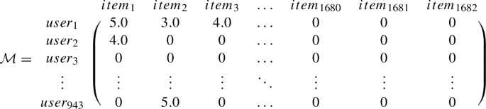
We use the MovieLens 100K dataset to conduct experiments, in which 943 users rated 1682 movies with a rating scale of 1–5, where 1 = bad and 5 = excellent. The total number of ratings reaches 100,000 because each user has a rating of at least 20 movies. For this paper, we do some simple processing on the MovieLens 100K data as follows:

• (1) Reading the initial data information through Python to construct a matrix $\mathcal {M} = \left( m_{ij}\right) _{943 \times 1682}$, where the value of $m_{ij}$ is estimated by the $i^{th}$ user on the $j^{th}$ item and $m_{ij} \in \left\{ 0,1,2,3,4,5\right\}$. Here, for the convenience of calculation, 0 means that the user has not provided a rating.

  

• (2) Some initial information statistics are shown in Table 5.

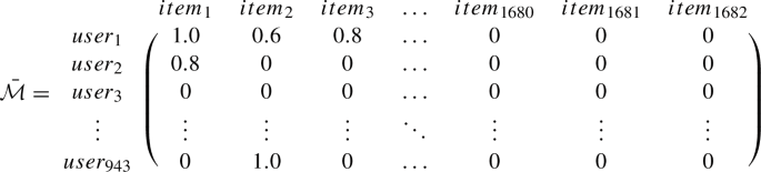
• (3) To apply the 3p-ASMs, the matrix needs to be normalized, that is, ratings are normalized to the value of the interval $\left[ 0, 1\right]$ as $\bar{\mathcal {M}}$ as follows:

  

4.2 The Applications of 3p-ASM

If a pair of comparison objects are exactly the same, that is, they have the same features and the same value, then the similarity is always equal to 1. However, if two objects are slightly different, for example, have different features or have the same features but have different values, compared with the proposed similarity measure, the existing similarity measure cannot more accurately identify their differences. To illustrate the advantages of 3p-ASM in overcoming this drawback, we focus on two aspects: (i) compare the similarity of between two users; omit processing the similarity between two items that are similar. (ii) Select K-nearest movies using KNN method based on proposed 3p-ASM.

4.2.1 Comparison with Classical Vector-Based Symmetric Similarity Methods

To simplify the whole calculation process, based on the fact that the values of the elements of the matrix $\bar{\mathcal {M}}$ belong to the interval $\left[ 0,1\right]$, we will apply the Eq. (26) to compute the similarity values between the two users of $\bar{\mathcal {M}}$. For example, selecting the first two rows, then $a = \left[ 1.0, 0.6, 0.8, \ldots , 0, 0, 0 \right]$ and $b = \left[ 0.8, 0, 0,\ldots , 0, 0, 0 \right]$. Thus, we will compute the results as follows:

$$\begin{aligned} \begin{aligned}&{S}_ \textbf{Cosine}\left( a,b\right) ={S}_ \textbf{Cosine}\left( b,a\right) =0.1669;\\&{S}^2_\textbf{Dice}\left( a,b\right) ={S}^2_\textbf{Dice}\left( b,a\right) =0.1303;\\&{S}^2_ \textbf{Jaccard}\left( a,b\right) ={S}^2_ \textbf{Jaccard}\left( b,a\right) =0.0697; \end{aligned} \end{aligned}$$

and

$$\begin{aligned} \mathcal {S}\left( a,b \right)= & {} 0.1068~\mathrm{{and}}~\mathcal {S}\left( b,a \right) \\= & {} 0.1392 ~\mathrm{{with}}~\left\{ \begin{array}{l} \alpha = 0.6758 \\ \gamma = 0.0999 \\ \beta = 0.2242 \\ \end{array}\right. . \end{aligned}$$

It should be noted here that $\mathcal {S}\left( a,b \right) \not =\mathcal {S}\left( b,a \right)$ for $\gamma \not = \beta$, and the similarity values of $\mathcal {S}\left( a,b \right)$ and $\mathcal {S}\left( b,a \right)$ are computed with the variation of the three condition parameters. For instance, if $\alpha = 0.0949$, $\gamma = 0.4677$ and $\beta = 0.4374$, then $\mathcal {S}\left( a,b \right) = 0.0070$ and $\mathcal {S}\left( b,a \right) = 0.0068$. In addition, to adjust the values of three conditional parameters, the similarity value of $\mathcal {S}\left( a,b \right)$ will be as close as possible to the values of ${S}_ \textbf{Cosine}\left( a,b\right)$, ${S}^2_\textbf{Dice}\left( a,b\right)$ and ${S}^2_ \textbf{Jaccard}\left( a,b\right)$. For example, choose the values of $\gamma ,\alpha ,\beta$ as $\alpha = 0.7755$, $\gamma = 0.0440$ and $\beta = 0.1805$, the similarity value is $\mathcal {S}\left( a,b \right) =0.1555$ that is close to ${S}_ \textbf{Cosine}\left( a,b\right)$.

In summary, the vector-based 3p-ASM, $\mathcal {S}\left( a,b \right)$, differs from the classical symmetric similarity measures mainly because different conditional parameters of $\mathcal {S}\left( a,b \right)$ lead to different computational results, which confirms the necessity of a parametric description of common and distinct features.

4.2.2 Application of KNN Method Based on 3p-ASM

In general, similarity measures are often used for classification, and the more commonly used method is KNN. Here, we use KNN for simple item-based classification. Without loss of generality, we consider two cases of applying the combination of Eqs. (18), (19) and (20): (i) for given two values, for instance $\gamma = 0.2$ and $\beta = 0.3$ (see Tables 6, 7); (ii) the three parameters vary randomly (see Table 8). For simplicity, we will find the 10 nearest neighbors of the term Copycat (1995) and its average ratings is 3.302325581395349.

Table 6 Case 1: Select 10 nearest neighbors items using the 3p-ASM $\mathcal {S}\left( a,b\right)$

Table 7 Case 1: Select 10 nearest neighbors items using the 3p-ASM $\mathcal {S}\left( b,a\right)$

Table 8 Case 2: Select 10 nearest neighbors items using the 3p-ASM $\mathcal {S}\left( a,b\right)$

Tables 6 and 7 are obtained by applying the 3p-ASM model $\mathcal {S}\left( a,b\right)$ and $\mathcal {S}\left( b,a\right)$ with given values $\gamma = 0.2$, $\beta = 0.3$ and $\alpha = 1-\gamma -\beta$. They have shared 6 movies and have 4 different movies because $\gamma = 0.2$ is close to $\beta = 0.3$ and their vectors of rating value is close to Copycat (1995)’s rating vector. Their different movies further indicate the two directions in which they imply: from object a to b and from object b to a. Furthermore, if $\gamma$ and $\beta$ are closer to each other, the results of 10 nearest items of $\mathcal {S}\left( a,b\right)$ and $\mathcal {S}\left( b,a\right)$ share more movies to each other, vice versa. For instance, let $\alpha = 0.7754$, $\gamma = 0.1023$ and $\beta = 0.1223$, then the results of $\mathcal {S}\left( a,b\right)$ and $\mathcal {S}\left( b,a\right)$ share 8 movies such as Aladdin and the King of Thieves (1996), Aladdin (1992), Goofy Movie, A (1995), Santa Clause, The (1994), Home Alone (1990), Aristocats, The (1970), D3: The Mighty Ducks (1996) and Love Bug, The (1969). Thus, when controlling the values of parameters, we can obtain an average closer to Copycat (1995)’s rating average value 3.302325581395349, as shown in Table 8. Overall, from the average results, the effectiveness of 3p-ASM models is further verified, the closer the results are between them, the more common features of the 10 nearest items are shared.

5 Conclusions and Future Work

In most practical situations, the similarity is not always symmetric, but asymmetric. To better departure the asymmetric, in this article, we were further studying 3-parameter-Tversky’s Ratio Model [5] to propose 3p-ASM models, which have made some contributions: (1) a novel parameter $\alpha$ has been added to characterize the common features between two compared objects. Thence, a new series of 3p-ASM models have been proposed that contain three conditional parameters satisfying $\alpha > 0$, $\gamma ,\beta \ge 0$, $\gamma \not =\beta$ and $\alpha +\gamma +\beta = 1$. (2) In the case of features’ values are estimated in $\left\{ 0,1\right\}$ and $\left[ 0,1\right]$, the proposed 3p-ASM models have been defined based on the concept of crisp set, fuzzy set and vector. The first two are an extension of the ratio model based on set theories, and the latter is based on vector theory. (3) We have studied some interesting properties, for example, a pair of parameters under a given parameter, whose influence on the final result has been studied mathematically and directly represented graphically; simulations and comparative analyses have also been performed.

It is well known that real-world problems are often posed under uncertainty, and these problems have been successfully modeled using fuzzy linguistic approaches [56,57,58]. Based on these, in future work, we shall straightforwardly extend the proposed ratio model to other representation contexts, such as intuitionistic fuzzy set [2], hesitant fuzzy set [45], hesitant fuzzy linguistic term set [38], and ELICIT [25], and the values of the features are not only those in $\left\{ 0,1\right\}$ or $\left[ 0,1\right]$. However, it is still an unsolved problem to choose the values of these three parameters and to satisfy the conditional constraints under uncertainty. To this end, it is possible to apply Robust to further investigate their uncertainty in the future.

References

Andrea Rodriguez, M., Egenhofer, M.J.: Comparing geospatial entity classes: an asymmetric and context-dependent similarity measure. Int. J. Geogr. Inf. Sci. 18(3), 229–256 (2004)
Atanassov, K.: Intuitionistic fuzzy sets. Int. J. Bioautom. 20(suppl. 1), 1–6 (2016)
Bag, S., Kumar, S.K., Tiwari, M.K.: An efficient recommendation generation using relevant Jaccard similarity. Inf. Sci. 483, 53–64 (2019)
Bao, J., Shen, J., Liu, X., Liu, H.: Quick asymmetric text similarity measures. In: Proceedings of the 2003 International Conference on Machine Learning and Cybernetics (IEEE Cat. No. 03EX693), vol. 1, pp. 374–379. IEEE (2003)
Bashon, Y., Neagu, D., Ridley, M.J.: Fuzzy set-theoretical approach for comparing objects with fuzzy attributes. In: 2011 11th International Conference on Intelligent Systems Design and Applications, pp. 754–759. IEEE (2011)
Cacheda, F., Carneiro, V., Fernández, D., Formoso, V.: Comparison of collaborative filtering algorithms: Limitations of current techniques and proposals for scalable, high-performance recommender systems. ACM Trans. Web (TWEB) 5(1), 1–33 (2011)
Cao, B., Yang, Q., Sun, J.T., Chen, Z.: Learning bidirectional asymmetric similarity for collaborative filtering via matrix factorization. Data Min. Knowl. Discov. 22(3), 393–418 (2011)
Chen, N., Xu, Z., Xia, M.: Interval-valued hesitant preference relations and their applications to group decision making. Knowl. Based Syst. 37, 528–540 (2013)
Cover, T., Hart, P.: Nearest neighbor pattern classification. IEEE Trans. Inf. Theory 13(1), 21–27 (1967)
Cui, L., Wu, J., Pi, D., Zhang, P., Kennedy, P.: Dual implicit mining-based latent friend recommendation. IEEE Trans. Syst. Man Cybern. Syst. 50(5), 1663–1678 (2018)
Dice, L.: Measures of the amount of ecologic association between species. Ecology 26(3), 297–302 (1945)
Duan, X., Tan, Z.H.: A spatial self-similarity based feature learning method for face recognition under varying poses. Pattern Recognit. Lett. 111, 109–116 (2018)
Dubois, D., Prade, H.: Fuzzy cardinality and the modeling of imprecise quantification. Fuzzy Sets Syst. 16(3), 199–230 (1985)
Elboher, E., Werman, M.: Asymmetric correlation: a noise robust similarity measure for template matching. IEEE Trans. Image Process. 22(8), 3062–3073 (2013)
Gawron, J.M.: Improving sparse word similarity models with asymmetric measures. In: Proceedings of the 52nd Annual Meeting of the Association for Computational Linguistics (Volume 2: Short Papers), Baltimore, Maryland, pp. 296–301. Association for Computational Linguistics (2014). https://doi.org/10.3115/v1/P14-2049
Gou, X., Xu, Z., Liao, H., Herrera, F.: Consensus model handling minority opinions and noncooperative behaviors in large-scale group decision-making under double hierarchy linguistic preference relations. IEEE Trans. Cybern. 51(1), 283–296 (2020)
Herrera, F., Martínez, L.: A 2-tuple fuzzy linguistic representation model for computing with words. IEEE Trans. Fuzzy Syst. 8(6), 746–752 (2000)
Huang, D., Wang, C.-D., Peng, H., Lai, J., Kwoh, C.-K.: Enhanced ensemble clustering via fast propagation of cluster-wise similarities. IEEE Trans. Syst. Man Cybern. Syst. 51(1), 508–520 (2018)
Hubert, L.: Min and max hierarchical clustering using asymmetric similarity measures. Psychometrika 38(1), 63–72 (1973)
Irlenbusch, B., Mussweiler, T., Saxler, D.J., Shalvi, S., Weiss, A.: Similarity increases collaborative cheating. J. Econ. Behav. Organ. 178, 148–173 (2020)
Jaccard, P.: Distribution de la flore alpine dans le bassin des dranses et dans quelques régions voisines. Bull. Soc. Vaud. Sci. Nat. 37, 241–272 (1901)
Kolahkaj, M., Harounabadi, A., Nikravanshalmani, A., Chinipardaz, R.: A hybrid context-aware approach for e-tourism package recommendation based on asymmetric similarity measurement and sequential pattern mining. Electron. Commer. Res. Appl. 42, 100978 (2020)
Krawczak, M., Szkatuła, G.: On asymmetric matching between sets. Inf. Sci. 312, 89–103 (2015)
Kunimoto, R., Vogt, M., Bajorath, J.: Maximum common substructure-based Tversky index: an asymmetric hybrid similarity measure. J. Comput. Aided Mol. Des. 30(7), 523–531 (2016)
Labella, Á., Rodríguez, R., Martínez, L.: Computing with comparative linguistic expressions and symbolic translation for decision making: ELICIT information. IEEE Trans. Fuzzy Syst. 20(10), 2510–2522 (2019)
Li, C., Dong, Y., Xu, Y., Chiclana, F., Herrera-Viedma, E., Herrera, F.: An overview on managing additive consistency of reciprocal preference relations for consistency-driven decision making and fusion: Taxonomy and future directions. Inf. Fusion 52, 143–156 (2019)
Li, J., Sang, N., Gao, C.: Completed local similarity pattern for color image recognition. Neurocomputing 182, 111–117 (2016)
Liu, D., Chen, X., Peng, D.: Cosine similarity measure between hybrid intuitionistic fuzzy sets and its application in medical diagnosis. Comput. Math. Methods Med. 2018, 3146873–3146877 (2018)
Liu, H., Hu, Z., Mian, A., Tian, H., Zhu, X.: A new user similarity model to improve the accuracy of collaborative filtering. Knowl. Based Syst. 56, 156–166 (2014)
Mi, J.X., Li, C., Li, C., Liu, T., Liu, Y.: A human visual experience-inspired similarity metric for face recognition under occlusion. Cogn. Comput. 8(5), 818–827 (2016)
Millan, M., Trujillo, M., Ortiz, E.: A collaborative recommender system based on asymmetric user similarity. In: International Conference on Intelligent Data Engineering and Automated Learning, pp. 663–672. Springer (2007)
Niwattanakul, S., Singthongchai, J., Naenudorn, E., Wanapu, S.: Using of Jaccard coefficient for keywords similarity. In: Proceedings of the International Multiconference of Engineers and Computer Scientists, vol. 1, IMECS 2013, Hong Kong, China, pp. 380–384 (2013)
Park, K., Hong, J.S., Kim, W.: A methodology combining cosine similarity with classifier for text classification. Appl. Artif. Intell. 34(5), 396–411 (2020)
Patra, B.K., Launonen, R., Ollikainen, V., Nandi, S.: A new similarity measure using Bhattacharyya coefficient for collaborative filtering in sparse data. Knowl. Based Syst. 82, 163–177 (2015)
Peng, X., Dai, J.: Algorithms for interval neutrosophic multiple attribute decision-making based on MABAC, similarity measure, and EDAS. Int. J. Uncertain. Quantif. 7(5): 395–421 (2017)
Pirasteh, P., Hwang, D., Jung, J.: Exploiting matrix factorization to asymmetric user similarities in recommendation systems. Knowl. Based Syst. 83, 51–57 (2015)
Ralescu, D.: Cardinality, quantifiers, and the aggregation of fuzzy criteria. Fuzzy Sets Syst. 69(3), 355–365 (1995). (Fuzzy Information Processing)
Rodríguez, R., Martínez, L., Herrera, F.: Hesitant fuzzy linguistic term sets for decision making. IEEE Trans. Fuzzy Syst. 20(1), 1109–119 (2012)
Rodríguez, R., Martínez, L., Herrera, F.: A group decision making model dealing with comparative linguistic expressions based on hesitant fuzzy linguistic term sets. Inf. Sci. 241(1), 28–42 (2013)
Rodríguez, R.M., Martínez, L., Herrera, F.: A group decision making model dealing with comparative linguistic expressions based on hesitant fuzzy linguistic term sets. Inf. Sci. 241, 28–42 (2013)
Salton, G., McGill, M.: An introduction to modern information retrieval (3rd print) (1987)
Santini, S., Jain, R.: Similarity measures. IEEE Trans. Pattern Anal. Mach. Intell. 21(9), 871–883 (1999)
Sato-Ilic, M., Sato, Y.: A general fuzzy clustering model based on asymmetric aggregation operators. IETE J. Res. 44(4–5), 207–218 (1998)
Singh, A., Kumar, S.: A novel dice similarity measure for IFSS and its applications in pattern and face recognition. Expert Syst. Appl. 149, 113245 (2020)
Torra, V.: Hesitant fuzzy sets. Int. J. Intell. Syst. 25(6), 529–539 (2010)
Tversky, A.: Features of similarity. Psychol. Rev. 84(4), 327 (1977)
Ureña, R., Chiclana, F., Morente-Molinera, J.A., Herrera-Viedma, E.: Managing incomplete preference relations in decision making: a review and future trends. Inf. Sci. 302, 14–32 (2015)
Wang, P., Liu, P., Chiclana, F.: Multi-stage consistency optimization algorithm for decision making with incomplete probabilistic linguistic preference relation. Inf. Sci. 556, 361–388 (2021)
Wang, Y., Deng, J., Gao, J., Zhang, P.: A hybrid user similarity model for collaborative filtering. Inf. Sci. 418, 102–118 (2017)
Wei, F., Vijayakumar, P., Kumar, N., Zhang, R., Cheng, Q.: Privacy-preserving implicit authentication protocol using cosine similarity for internet of things. IEEE Internet Things J. 8(7), 5599–5606 (2020)
Wei, G.: Some cosine similarity measures for picture fuzzy sets and their applications to strategic decision making. Informatica 28(3), 547–564 (2017)
Wei, G.: The generalized dice similarity measures for multiple attribute decision making with hesitant fuzzy linguistic information. Econ. Res. (Ekonomska istraživanja) 32(1), 1498–1520 (2019)
Wu, Y., Hu, H., Li, H.: Age-invariant face recognition using coupled similarity reference coding. Neural Process. Lett. 50(1), 397–411 (2019)
Ye, J.: Cosine similarity measures for intuitionistic fuzzy sets and their applications. Math. Comput. Model. 53(1–2), 91–97 (2011)
Yen, C.Y., Cios, K.J.: Image recognition system based on novel measures of image similarity and cluster validity. Neurocomputing 72(1–3), 401–412 (2008)
Zadeh, L.A.: The concept of a linguistic variable and its application to approximate reasoning (i). Inf. Sci. 8(3), 199–249 (1975)
Zadeh, L.A.: The concept of a linguistic variable and its application to approximate reasoning (ii). Inf. Sci. 8(4), 301–357 (1975)
Zadeh, L.A.: The concept of a linguistic variable and its application to approximate reasoning (iii). Inf. Sci. 9(1), 43–80 (1975)
Zhang, Y., Yin, C., Wu, Q., He, Q., Zhu, H.: Location-aware deep collaborative filtering for service recommendation. IEEE Trans. Syst. Man Cybern. Syst. 51(6), 3796–3807 (2019)
Zielman, B., Heiser, W.J.: Models for asymmetric proximities. Br. J. Math. Stat. Psychol. 49(1), 127–146 (1996)
Funding
This work is partially supported by the Spanish Ministry of Economy and Competitiveness through the Postdoctoral fellow Ramón y Cajal (RYC-2017-21978), the Andalucía Excellence Research Program with Research Project ProyExcel_00257 and the National Natural Science Foundation of China (62006154 and 72171182).
Author information
Authors and Affiliations
Contributions
Conceptualization, WH, BD, YYL and RMR; methodology, WH, BD and YYL; validation, RMR and YYL; formal analysis, WH, RMR and BD; investigation, WH, RMR and YYL; writing—original draft preparation, WH, BD and YYL; supervision, RMR and YYL; funding acquisition, RMR and YYL. All the authors have read and agreed to the published version of the manuscript.
Corresponding author
Ethics declarations
Conflict of Interest
The authors declare no conflict of interest.
Rights and permissions
Open Access This article is licensed under a Creative Commons Attribution 4.0 International License, which permits use, sharing, adaptation, distribution and reproduction in any medium or format, as long as you give appropriate credit to the original author(s) and the source, provide a link to the Creative Commons licence, and indicate if changes were made. The images or other third party material in this article are included in the article’s Creative Commons licence, unless indicated otherwise in a credit line to the material. If material is not included in the article’s Creative Commons licence and your intended use is not permitted by statutory regulation or exceeds the permitted use, you will need to obtain permission directly from the copyright holder. To view a copy of this licence, visit http://creativecommons.org/licenses/by/4.0/.
About this article
Cite this article
He, W., Dutta, B., Liu, Y. et al. Extend Tversky’s Ratio Model to an Asymmetric Similarity Measurement Model with Three Conditional Parameters: 3p-ASM Model. Int J Comput Intell Syst 16, 113 (2023). https://doi.org/10.1007/s44196-023-00285-8
Received:
Accepted:
Published:
DOI: https://doi.org/10.1007/s44196-023-00285-8