
Abstract
With the aim to enhance prediction accuracy for nonlinear time series, this paper put forward an improved deep Echo State Network based on reservoir states reconstruction driven by a Self-Normalizing Activation (SNA) function as the replacement for the traditional Hyperbolic tangent activation function to reduce the model’s sensitivity to hyper-parameters. The Strategy was implemented in a two-state reconstruction process by first inputting the time series data to the model separately. Once, the time data passes through the reservoirs and is activated by the SNA activation function, the new state for the reservoirs is created. The state is input to the next layer, and the concatenate states module saves. Pairs of states are selected from the activated multi-layer reservoirs and input into the state reconstruction module. Multiple input states are transformed through the state reconstruction module and finally saved to the concatenate state module. Two evaluation metrics were used to benchmark against three other ESNs with SNA activation functions to achieve better prediction accuracy.
1 Introduction
A prediction is a statement about forecasting an event or data in the future. Based on a general belief that what happened before will happen again, people often look at history to provide them with clues to plan for the future. However, reliable prediction on nonlinear time series is a complex task [1, 2]. Given the capability of time series in retaining features of events or data in the sequence of time as events unfold, it has become a source of information to trace the footstep of history over time, to allow us to study and identify key factors that drive the development. As a result, many algorithms [3, 4] have been developed over the years to study prediction using time series, as a source of historical information to learn about the past, and seek to uncover key underlying features or patterns hidden within the data set to make predictions for the future. However, the time series data set is inherently nonlinear, which makes it challenging to analyze. Tools like artificial neural networks have shown promising potential in learning and predicting nonlinear data [5]. Among them, recurrent neural network (RNN) has been widely reported in conjunction with time series as the data sets [6, 7].
Nonetheless, limitations do exist in handling training of bifurcation towards convergence, which when the time span becomes larger or as the network deepens, the calculation will grow exponentially to require the support of massive computational power [8]. Furthermore, exploding and vanishing gradients may also occur when using RNN [9]. This has led many researchers to look for an alternative to recurrent neural networks, known as reservoir computing (RC), the model offers a higher efficiency, and better solution to overcome convergence of bifurcation and gradient limitations of the recurrent neural network (RNN) [10, 11].
Reservoir computing is a framework of computation derived from recurrent neural network theory that maps input signals into higher dimensional computational spaces through the dynamics of a fixed, but non-linear system called a reservoir. After the input signal is fed into the reservoir, which is treated as a “black box,” a simple readout mechanism is trained to read the state of the reservoir and map it onto the desired output. The first key benefit of this framework is that the training is performed only at the readout stage when the reservoir dynamics are already fixed. The other advantage is the requirement for computational power is not demanding, and could be supportable with a normal PC or laptop.
The concept of reservoir computing stems from the use of recursive connections within neural networks to create a complex dynamical system. It is a generalization of earlier versions of neural network architectures such as recurrent neural networks, Liquid State Machine (LSM), or Echo State Networks (ESN). Reservoir computing has also extended over to apply to physical systems that are not neural networks in the classical sense, but rather continuous systems in space and/or time: e.g., a literal “bucket of water” can serve as a reservoir that performs computations on inputs given as perturbations of the surface. The resultant complexity of such recurrent neural networks was found to be useful in solving a variety of problems including language processing and dynamic system modeling. However, training of recurrent neural networks is challenging and computationally extensive, and therefore, switching over to Reservoir computing reduces those training-related challenges by fixing the dynamics of the reservoir to only train on the linear output layer. A large variety of nonlinear dynamical systems can serve as a reservoir that performs computations.
As the special computational framework of RNN, reservoir computing (RC) has a complete theoretical basis and can effectively avoid the problems of high computational complexity and gradient explosion or vanishment. There are two main types of RC, namely Echo State Networks (ESN) and Liquid State Machine (LSM). They could be easy to train to deliver excellent predictions. Hence, they are widely applied to areas such as system identification, signal processing, and time series prediction. In this article, we will present the ESN, and its potential to convert the input information into a high-dimensional signal to be stored in its reservoirs, and for the delivery of better prediction, based on training on nonlinear time series data sets. Difference from other RNN methods, ESN only needs to adjust the output weight matrix with a linear regression algorithm, which makes it easy to implement and could be supported with low computational requirements. Although, ESN is widely applied in solving complex data-based problems, such as classification[12], and time series forecasting [13], it does suffer from sensitivity to hyperparameters [14]. To address this problem, some researchers have opted for changing the model’s topology or adjusting the sampling method of time series to extract the features of time series in various ways with little improvement to show. Here, we propose a two-state reconstruction method to train the system to redo the training on the same set of data to learn and extract missing temporal features from the existing data set, rather than mining new ones. At the same time, we will also replace the tanh activation function in ESN with an SNA activation function to ensure that the model runs in a stable state.
The remainder of this paper is organized as follows. Section 2 summarizes the current works on the time series prediction on ESN. In Section 3, we will present the operation mechanism of the original ESN. In In Sect. 5, we will showcase the use of the SNA activation function to enable the ESN to extract temporal features from the existing state in the reservoir in a stable environment. A bench-marking will be presented in Section 5, with results showcased in Sect. 6.
2 Literature review
ESN has exhibited its robustness in nonlinear mapping to predict accurately at a faster speed than others, making it an ideal model for predicting nonlinear time series [13, 15].
ESN was first introduced to time series problems in 2004 when it was shown to be capable of working work with nonlinear data in chaotic wireless communication systems to predict accurately [16]. Thereafter, when a leakage rate was added onto the standard ESN as a parameter to optimize learning different time features at the global level, it has come up head-and-shoulder on top of many other classic counterparts, especially when it is placed to work with noisy time series, and time-warped dynamic patterns data sets [17]. However, in the traditional single-layer random connected reservoir, there is a limitation on how long it could preserve the features of long-term time series. Over time, the time features in the reservoir gradually disappear, and this has limited ESN’s scope for expanding. To overcome this limitation on maintaining the long-term memory capacity of the reservoir, a variety of algorithms such as Deep ESN, and some hybrid models that combine ESN with other algorithms have been attempted, with little results to show for [5]. There were also others who proposed the use of the Principal Neuron Reinforcement (PNR) algorithm [18] to strengthen the connections between the main neuron and other neurons, hoping that this might improve the performance. The introduction of Anti-Oja (AO) [19] was yet another attempt to learn to update neuron weights in the reservoir, by reducing the correlation between neurons, to improve the dynamic to diversify of internal state, with the hope that it would improve the prediction performance. In an attempt to simplify the internal structure of the reservoir, Simple Cycle Reservoir (SCR), Delay Line Reservoir (DLR), and Delay Line Reservoir with feedback connections (DLRB) were reported in 2010 [20], and seem to delivery better performance as expected. Thereafter, adjacent-feedback Loop Reservoir (ALR) [13] introduced the feedback mechanism of adjacent neurons on SCR and achieved satisfactory results.
For Deep ESN, which consists of multiple stacked reservoirs, focuses were directed to create additional layers inside the reservoirs to increase the richness in features and improve the performance [11]. Researchers have also found better accuracy by stacking multiple layers of reservoirs to improve the short-term memory capacity. Based on this observation, a Deep ESN, [21] with a new hidden layer was proposed by adding three gate states inside the reservoirs, to improve the knowledge held in deep memory. Compared with Deep ESN, Deepr-ESN[22] continuously works on developing the high-level state space in the reservoirs by new rounds of training to learn additional features from the low-level feature space, in the process, remove the high-frequency components of the representations, and resulted in significant improvement over other similar models.
Modular Deep ESN (Mod-Deep ESN) [23] proposed several models with heterogeneous topology to capture multi-scale dynamic features of time series. Mod-Deep ESN used Criss-Cross topology and Wide Layered topology were proposed to train on some time series to prepare for prediction tasks. Multi-reservoir ESN with sequence re-sampling (MRESN) [24] deployed three re-sampling methods based on Deep ESN and Group ESN to improve the prediction performance for nonlinear time series. In [25], three ESN models integrated SNA have given birth to the arrival of the Deep ESN with SNA, Group ESN with SNA, and Grouped Deep ESN with SNA, to overcome the ESN model’s sensitivity to hyper-parameters.
ESN not only be driven by deep learning but could also incorporate other machine learning algorithms and neural networks into the system, to enhance the linkage between information sensed in from the environment (sensation) with features held in the reservoirs (perception) to provide a sense of continuity of experience. Such continuity may even serve as the basis for personal identity. In [26], the feed-forward neural network is used to replace the output layer of ESN, and the back-propagation algorithm is used to optimize the feed-forward neural network.
In 2019, Sun X, et al. put forward an enhanced echo-state restricted Boltzmann machine (eERBM) [12] to extract temporal features through a restricted Boltzmann machine and then input them into ESN. Through experiments, eERBM yields a better nonlinear approximation and delivers accurate prediction in traffic tasks. Others like He K, et al. decided to opt for improvement on the Long-term performance prediction for proton exchange membrane fuel cell (PEMFC) in vehicles based on a least absolute shrinkage and selection operator (LASSO-ESN) [27] to eliminate the parameters with the minimum weight during the prediction process to improves the accuracy of the prediction.
In this review, we found that most ESN we have covered so far, mainly focus on the increasing number of reservoir states, instead of paying attention on extracting more time features from the existing time series data set to develop new states for the reservoir. Inspired by the works of Li Z, et. al. on multi-reservoir echo state networks with sequence re-sampling for nonlinear time-series prediction [24], we propose an improved ESN that will generate new states through a state reconstruction process using features extracted between different layers of the reservoir. This hypothesis would be tested in the numerical simulation in Section 5, when we brandmark it with the other three deep models featured in [25].
3 Preliminaries of ESN
ESN is a particular recurrent neural network proposed by Jaeger [28]. The architecture of a traditional ESN shown in Fig. 1 which consists of an input layer, a reservoir with sparse connections, and a readout layer. \(W_{\mathrm{in}}\) represents the weight matrix of the input unit, W is the weight inside the reservoir, and \(W_{\mathrm{out}}\) is the weight of the output unit. \(W_{\mathrm{in}}\) and W are generated from random values, and they are fixed during training. The \(W_{\mathrm{out}}\) is obtained by linear regression, which can dramatically reduce the amount of calculation compared to RNN.

Traditional ESN
The input units, reservoir units, and output units are denoted by:
The updated formula of neurons in the reservoirs is as follows:
where f is the activation function, traditional ESN uses tanh to activate neurons. The prediction output calculation formula is as follows:
where \(f_{\mathrm{out}}\) is the readout function and \(W_{\mathrm{out}}\) is the trained output weight matrix. Symbol \([\cdot;\cdot ]\) stands for a vertical concatenation.
To ensure the dynamic stability of the network during initialization, ESN needs to satisfy the asymptotic stability property, which is called Echo State Property (ESP) [29]. To guarantee ESP, the spectral radius of the reservoir’s weight matrix (Equation (6)) needs to be less than 1.
where \(W_{1}\) is the randomly generated reservoir weight matrix, \(\lambda _{\mathrm{max}}\) is the spectral radius of \(W_{1}\), and α is the scaling parameter for tuning.
4 The framework of proposed ESN model
This paper will focus on the issue of sensitivity of the ESN’s regarding hyperparameters that prevent them from working in a stable environment to work on generating more states for the reservoir by training to learn additional temporal features from the states in the reservoir. In other words, the goal to enhance the prediction accuracy of Echo State Networks (ESN), will now decompose into two objectives; Firstly, it is on the identification of a replacement for the hyperbolic tangent activation function to ensure the ESN is given to operate in a stable environment. Secondly, to improve the predictivity of ESN, additional training to enrich the reservoirs with additional temporal features learned from pairs of states selected from the activated multi-layer reservoirs and input into the state reconstruction module.
The proposed ESN is developed based on Deep ESN, and its schematic diagram is shown in Figure 2 as the proposed improved version of ESN. First, we replace the traditional Hyperbolic tangent activation function with a SNA activation function to reduce the impact due to the sensitivity of hyperparameters. Then, we design a state reconstruction module based on Deep ESN. The proposed ESN model aims to extract additional features from the existing states stored between different layers in ESN.

Comparison of Deep ESN and our proposed ESN
The time series forecasting process of the proposed ESN is as follows (see Fig. 3):
-
1.
Input the time series data to the model separately.
-
2.
After the time data passes through the reservoirs and is activated by SNA activation function (Subsect. 4.1), the state of the reservoirs is obtained. The state is input to the next layer, and the concatenate states module (Subsect. 4.3) saves.
-
3.
Pairs of states are selected from the activated multi-layer reservoirs and input into the state reconstruction module (Subsect. 4.2). Multiple input states are transformed through the state reconstruction module, and finally saved to the concatenate states module.
-
4.
Predict future time data through ridge regression.

Flowchart of the proposed ESN’s training process
4.1 Self-normalizing activation function on hyper-sphere
Generally, the traditional ESN model uses tanh as the reservoir activation function. This activation function is simple and practical, whereas it is very sensitive to hyperparameters. Only proper hyperparameter configurations can ensure that the ESN is at the edge of criticality and maximize the ESN’s performance. Otherwise, the network will be useless and result in chaotic behavior. Therefore, we use the SNA activation function (Equation (7)) rather than tanh in the ESN. Theoretical analysis of the SNA activation function shows that the maximum Lyapunov exponent of the model is always zero. It means that no matter how the hyperparameters of the network are configured, the model always runs in a stable state, eliminating the excessive dependence on hyperparameters [14]. Furthermore, SNA guarantees that ESN exhibits nonlinear behavior and handles tasks that require rich dynamics. SNA also provides memory behavior similar to linear networks, effectively balancing non-linearity and memory ability [14].
In Equation (7), \({\alpha}_{k}\) is the pre-activation vector obtained from the state \({x_{k-1}}\) of the input \({u_{k}}\). In Equation (8), the pre-activation vector \({\alpha}_{k}\) is projected onto an \(N-1\) dimensional hypersphere with radius r, and the post-activation state \({x_{k}}\) is obtained. The SNA activation function is not element-wise, it depends on all the states, and it is a global activation function. The activation function of each neuron depends on the values of other neurons.
4.2 States reconstruction module
We design the state reconstruction module based on Deep ESN, as shown in Fig. 4. The states reconstruction module is used to cross-stitch the original states of the input in the original order. Unlike general Deep ESN, we further process the state of the reservoir that has been obtained, expecting to obtain more temporal features. As shown in Fig. 2(b), after inputting the data into the multi-layer ESN model from the top, the states are inputted to the state reconstruction module in pairs, extracting more temporal features. We employ \(s(\kappa ) \in \mathbb{R}^{N_{r}}\) for \(r = 1,2...,{N_{r}}\) to represent the inputs to the state reconstruction module, where \(N_{r}\) is the size of the reservoirs. And then, a collection matrix of the inputs in pair can be defined as \(S_{1} = [s_{1}(1),s_{1}(2),\ldots s_{1}(N_{r})]\), \(S_{2} = [s_{2}(1),s_{2}(2),\ldots s_{2}(N_{r})]\). Based on the sampling and splicing of states, we put forward two-state reconstruction methods: single adjacent elements concatenation and double adjacent elements concatenation, respectively. They are designed to realize the mutual mixing of the states of different layers and improve the model’s ability to extract the features of time series.

An example of state reconstruction of two states in the proposed ESN
Concatenation of single adjacent elements
Regarding the method of a single adjacent element, it inputs the states between the two layers into the state reconstruction module. It divides the elements into two states according to whether the subscript is odd or even. It keeps the relative position of reservoir states unchanged. The odd subscript elements of the first state are combined with the even subscript elements of the second state. The even subscript elements of the first state are combined with the odd subscript elements of the second state.
with
where τ represents the index of the original state element, and \({s_{\mathrm{rec}}}\) represents the new state after reconstruction. We construct \({s_{\mathrm{rec}1}}\) by interval sampling, and exchange index to construct \({s_{\mathrm{rec}2}}\).
Concatenation of double adjacent elements
This method treats two adjacent states as a group. They are concatenating odd-numbered combinations in the first state with even-numbered combinations in the second state and vice versa.
with
G represents the index formed by every two states as a group.
Through these two reconstruction methods, we can add several new states to the original states and ensure that the relative positions of the elements in the original states remain unchanged in the new states.
4.3 States concatenation module
In the states concatenation module, all states corresponding to time t are vertically connected. The vertically arranged states include the SNA-activated states and the new state obtained by the state reconstruction module.
The definition of states concatenation is as follows.
5 Numerical experiments
In this section, we undertook a number of simulations to study the outputs from the proposed ESN model, in comparison with its peers; namely ESN model with SNA, which is Deep ESN, Group ESN, and Grouped Deep ESN [30]. in terms of their accuracy in predicting on a set of multiple classical chaotic time series.
In here, Group ESN is a parallel shallow ESN model. While Deep ESN is composed of multiple ESNs stacked vertically, which are organized differently from the traditional deep neural networks, the output of Deep ESN is composed of the intermediate state of each layer. On the other hand, the Grouped Deep ESN is made up of Group ESN and Deep ESN, combined into one system with the aim of integrating the breadth and depth of both models.
During the simulations; a time series was fan-in into all four ESNs at the same time with their output fan-out separately at the final output stage. The improved ESN we proposed is mainly based on Deep ESN with the tanh activation function replaced by SNA activation function, to improve the stability of the ESN to oversee the state reconstruction module for the state enrichment by extracting more temporal features from the existing time series data set, hopefully to improve the prediction performance.
5.1 Dataset description
We use two benchmark prediction tasks named Multiple Superimposed Oscillators (MSO) and the Rossler system to evaluate the proposed ESN. Further, Laser and Electromyograms (EMG), which are two real data sets, are also applied to simulate time series prediction tasks (see Fig. 5). These four data sets are classic data sets in time series forecasting tasks. Among them, the first two data sets can be shown by mathematical expressions that their curves are smoother and therefore tend to be better predicted. The latter two data sets are extracted from real scenes, have a certain degree of chaos, and are difficult to predict.

Partial display of MSO12,Rossler,Laser, and EMG datasets
-
1.
MSO
MSO [31] is formed by superpositioning multiple sine signals of different frequencies.
$$\begin{aligned} {y(t) = \sum_{k=1}^{m}\sin(\omega _{k} t)}. \end{aligned}$$(16)Where m represents the number of different sine functions, and \({\omega _{k}}\) represents different frequencies. In the experiments, we perform one-step ahead predictions on superimposed sine signals of 12 different frequencies: \({\omega _{1}} = 0.2\), \({\omega _{2}} = 0.331\), \({\omega _{3}} = 0.42\), \({\omega _{4}} = 0.51\), \({\omega _{5}} = 0.63\), \({\omega _{6}} = 0.74\), \({\omega _{7}} = 0.85\), \({\omega _{8}} = 0.97\), \({\omega _{9}} = 1.08\), \({\omega _{10}} = 1.19\), \({\omega _{11}} = 1.27\), \({\omega _{12}} = 1.32\).
-
2.
Rossler system
The Rossler system [32] consists of three nonlinear ordinary differential equations that define a continuous-time dynamical system.
$$\begin{aligned} \textstyle\begin{cases} {\dfrac{dx}{dy} = -y-z}, \\ {\dfrac{dy}{dz} = x+ay}, \\ {\dfrac{dz}{dt} = b+z(x-c)} \end{cases}\displaystyle \end{aligned}$$(17)The system shows chaotic behavior for \(a=0.15, b=0.2, c=10\).
The time series of the Rossler system is generated with initial values \((-1, 0, 3)\) and step of 0.01. In our experiments, we make a one-step ahead prediction for \(\mathit{Rossler}-x(t)\).
-
3.
Laser
Santa Fe Laser Dataset is a benchmark dataset in time series forecasting tasks [33]. It is a real-world dataset measured in the laboratory with periodic laser output power datasets, and it contains a length of 10092. It will be used in one step ahead prediction of our simulation.
-
4.
EMG
Electromyography is mainly used in clinical experiments to assess functions such as muscles and nerves. We use the EMG time series of a 44-year-old healthy male with no history of muscle disease collected in work [34] and use it for one-step-ahead prediction.
We employ the same length of the training set, validation set, test set, and initial transient set on the above four experimental datasets. The specific parameters are shown in Table 1.
Each dataset is 4000 in length, of which the first 3000 data are used for training, 500 data are used for validation, and the last 500 data points are used for testing. The transient data set is 30. For a fair comparison, the same dataset partitioning is used in our improved ESN model and the three contrasting models.
5.2 Evaluation metrics
Two metrics are used to evaluate our model, root-mean-square error (RMSE) in Equation (18) and normalized root mean square error (NRMSE) in Equation(19). They have a strong theoretical correlation in statistical modeling and are the most commonly used measurement methods in time series prediction tasks [35].
\(y(t)\) refers to the actual data observed at time t under the length of \(N_{T}\), \(\hat{y(t)}\) refers to the predicted value at time t, and \(\bar{y(t)}\) represents the average value of real data.
5.3 Experiments settings
The parameter settings of the simulated ESNs are shown in Table 2. The input scaling θ, the spectral radius ρ, the density of internal weight η, the leaking rate α, and the regularizing factor β. The reservoir size \(N_{R}\) is varied in the range of \([100,1000]\) with the interval of 100. The activation radius r is in range \([10,50,100,\ldots,800]\).
After using the SNA activation function, the sensitivity of the input scaling θ and spectral radius ρ decreases. We can fix these two values to improve the search efficiency [25]. However, SNA function also introduces another hyperparameter, the activation radius r. Thus, for each dataset, we test the reservoir size \(N_{R}\) ∈ [100,200,…,1000] and the SNA activation radius r ∈ \([10,50,100,200,\ldots,800]\).
The improved ESN is compared with three models with SNA activation functions proposed in the work [30], Deep ESN with SNA, Grouped Deep ESN with SNA, and Grouped ESN with SNA. We use a grid search strategy to test each model under the same conditions and compare their optimal values.
5.4 Results analysis
In this section, we present and analyze the performance of our improved ESN and compare ESN models on the aforementioned four datasets. The optimal parameters of our proposed model in each dataset are shown in Table 3, Table 4, Table 5, and Table 6.
-
MSO
Table 3 lists the optimal performance of our improved model and the three comparative models under the optimal configuration within the given range. In this dataset, the average NRMSE (18) and RMSE (19) obtained by grouped ESN are the best, and the improved ESN is better than the other two models. Figure 6(b) shows the result of our improved model by grid search. Among them, \(N_{r}=600\), \(r=80\). The predicted time series is shown in Fig. 6(a).
Figure 6 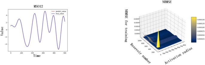
The prediction performance and grid search result on MSO12
Table 3 Hyperparameter setting in MSO task -
Rossler system
Table 4 shows that the proposed model outperforms other compared models on the Rossler system. The best prediction results of our proposed method are obtained under the parameter conditions: \(N_{R}=10\), \(r=300\). The grid search results and prediction are shown in Fig. 7.
Figure 7 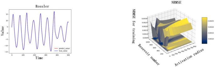
The prediction performance and grid search result on Rossler
Table 4 Hyperparameter setting in Rossler task -
Laser
The results of the Laser dataset are shown in Table 5. The improved ESN is still better than the three comparison models in RMSE and NRMSE, where the model parameters \(N_{R}=\)600, \(r=100\). The prediction and grid search results are shown in Fig. 8.
Figure 8 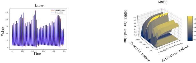
The prediction performance and grid search result on Laser
Table 5 Hyperparameter setting in Laser task -
Electromyograms
The experimental results of RMSE the EMG dataset are shown in Table 6. The result of RMSE standard deviation (18) obtained through multiple experiments on Deep ESN is slightly smaller than the ESN we proposed. The improved ESN is better than the comparison model on the rest of the metrics. The optimal parameter configuration is \(N_{R}=100\), \(r=800\). The predicted effect is shown in Fig. 9.
Figure 9 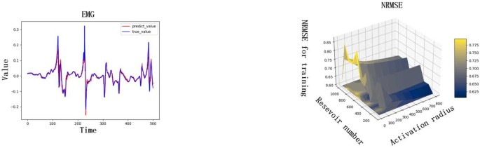
The prediction performance and grid search result on EMG
Table 6 Hyperparameter setting in EMG task


As we can see from the graphs generated by the simulation, the real curves of the MSO and Rossler systems are smoother, indicating that the four models predicted on these two data sets are more accurate, and the lines are almost completely fitted. As for Laser and Electromyograms, due to the many changes and poor regularity, the performance on these two data sets was somewhat lower with the larger. error.
Compared with the other three ESNs with SNA activation function, our improved ESN model has shown to perform rather well in the case of multiple indicators on the four data sets. Especially in comparison with the Deep ESN model, our model is better than Deep ESN in almost all indicators. The possible reason is that after state reconstruction, it seems to be able to capture rather more features.
On all four data sets we have selected, the minimum RMSE (18) and NRMSE (19) obtained by our model are the best among all. The improvement could be credited to the use of the state reconstruction module we proposed to capture additional relevant features from the time series by re-training on the states from the multi-layer reservoirs and re-splicing it in sequence during reconstruction. Compared with the original model, the state reconstruction module increases the richness of the original states. Although on the MSO data set, the average values of our NRMSE and RMSE are slightly lower than some of the peers, the performance of our model has been improved from a global view.
6 Conclusions
With the aim to improve the prediction accuracy for Echo State Networks (ESN) on nonlinear time series, we identified the instability due to the hyperbolic tangent activation function and the lack of temporal features existing within the states in reservoirs as two potential areas that in need of investigation.
Theoretical analysis of the SNA activation function shows that the maximum Lyapunov exponent of the model is always zero. It means that no matter how the hyperparameters of the network were configured, the model will always run in a stable state, as a result, eliminate the excessive dependency on hyper-parameters, and hence, the replacement of hyperbolic tangent activation function should provide us with the stability needed for our ESNs on work on the second problem.
Strategically, the issue of missing temporal features could be made up by re-training the existing states sitting inside the reservoirs to extract these features to create new states in a two-state reconstruction method as follows.
-
Input the time series data to the model separately.
-
After the time data passes through the reservoirs and is activated by SNA activation function, the state of the reservoirs is obtained. The state is input to the next layer, and the concatenate states module saves.
-
Pairs of states are selected from the activated multi-layer reservoirs and input into the state reconstruction module. Multiple input states are transformed through the state reconstruction module and finally saved to the concatenate states module.
The design of the state reconstruction module is based on Deep ESN that is used here to cross-stitch the original states of the input in the original order. After inputting the data into the multi-layer ESN model from the top, the states are inputted to the state reconstruction module in pairs, extracting more temporal features to concatenate them in a two-state reconstruction method: single adjacent elements concatenation and double adjacent elements concatenation, respectively. They are designed to realize the mutual mixing of the states from different layers to improve the model’s ability to extract these additional features from the time series concerned.
During the state concatenation module, all states corresponding to the time t are vertically connected. The vertically arranged stated include the SNA-activated stares and the next state objected by the state reconstruction module.
The proposed model was benchmarked with four popular improved ESN models; namely Deep ESN with SNA, Group Deep ESN with SNA, and Grouped ESN with SNA, on four time series data sets; namely Multiple Superimposed Oscillators [MSO], Rossler system, Santa Fe Laser Dataset, and EMG time series, to obtain a set of very interesting results in prediction performance among all its peers.
However, limitations do exist in this study that each layer’s state is reconstructed monolithically when layers of the reservoir might contains different hidden features in the time series, but were treated by us uniformly of the same type, which opened the way for future investigation to study the benefit from different architectural orientations that we might have missed in this study.
Availability of data and materials
This paper does not involve any data or material.
Code availability
There is no code for this manuscript.
References
M. Casdagli, Nonlinear prediction of chaotic time series. Phys. D, Nonlinear Phenom. 35(3), 335–356 (1989)
Z. Hajirahimi, M. Khashei, Hybrid structures in time series modeling and forecasting: a review. Eng. Appl. Artif. Intell. 86, 83–106 (2019)
N.I. Sapankevych, R. Sankar, Time series prediction using support vector machines: a survey. IEEE Comput. Intell. Mag. 4(2), 24–38 (2009). https://doi.org/10.1109/MCI.2009.932254
G. Heydari, M.A. Vali, A.A. Gharaveisi, Chaotic time series prediction via artificial neural square fuzzy inference system. Expert Syst. Appl. 55, 461–468 (2016)
C. Sun, M. Song, S. Hong et al., A review of designs and applications of echo state networks (2020). arXiv preprint. arXiv:2012.02974
J.L. Elman, Finding structure in time. Cogn. Sci. 14(2), 179–211 (1990)
D.E. Rumelhart, G.E. Hinton, R.J. Williams, Learning internal representations by error propagation, California Univ. San Diego La Jolla Inst. for Cognitive Science, 1985
K. Doya, Bifurcations in the learning of recurrent neural networks 3. Learn. (RTRL) 3, Article ID 17 (1992)
R. Grosse, Lecture 15: Exploding and Vanishing Gradients (University of Toronto Computer Science, 2017)
M. Lukoševičius, H. Jaeger, Reservoir computing approaches to recurrent neural network training. Comput. Sci. Rev. 3(3), 127–149 (2009)
C. Gallicchio, A. Micheli, L. Pedrelli, Deep reservoir computing: a critical experimental analysis. Neurocomputing 268, 87–99 (2017)
Q. Ma, L. Shen, W. Chen et al., Functional echo state network for time series classification. Inf. Sci. 373, 1–20 (2016)
X. Sun, H. Cui, R. Liu et al., Modeling deterministic echo state network with loop reservoir. J. Zhejiang Univ. Sci. C 13(9), 689–701 (2012)
P. Verzelli, C. Alippi, L. Livi, Echo state networks with self-normalizing activations on the hyper-sphere. Sci. Rep. 9(1), 1–14 (2019)
Z. Li, T. Tanaka, HP-ESN: echo state networks combined with Hodrick–Prescott filter for nonlinear time-series prediction, in 2020 International Joint Conference on Neural Networks (IJCNN) (IEEE Press, New York, 2020), pp. 1–9
H. Jaeger, H. Haas, Harnessing nonlinearity: predicting chaotic systems and saving energy in wireless communication. Science 304(5667), 78–80 (2004)
H. Jaeger, M. Lukoševičius, D. Popovici et al., Optimization and applications of echo state networks with leaky-integrator neurons. Neural Netw. 20(3), 335–352 (2007)
H.T. Fan, W. Wang, Z. Jin, Performance optimization of echo state networks through principal neuron reinforcement, in 2017 International Joint Conference on Neural Networks (IJCNN) (IEEE Press, New York, 2017), pp. 1717–1723
Š. Babinec, J. Pospíchal, Improving the prediction accuracy of echo state neural networks by anti-Oja’s learning, in International Conference on Artificial Neural Networks (Springer, Berlin, 2007), pp. 19–28
A. Rodan, P. Tino, Minimum complexity echo state network. IEEE Trans. Neural Netw. 22(1), 131–144 (2010)
Y. Yang, X. Zhao, X. Liu, A novel echo state network and its application in temperature prediction of exhaust gas from hot blast stove. IEEE Trans. Instrum. Meas. 69(12), 9465–9476 (2020)
Q. Ma, L. Shen, G.W. Cottrell, DeePr-ESN: a deep projection-encoding echo-state network. Inf. Sci. 511, 152–171 (2020)
Z. Carmichael, H. Syed, S. Burtner et al., Mod-deepesn: modular deep echo state network (2018). arXiv preprint. arXiv:1808.00523
Z. Li, G. Tanaka, Multi-reservoir echo state networks with sequence resampling for nonlinear time-series prediction. Neurocomputing 467, 115–129 (2022)
R. Wcisło, W. Czech, Grouped multi-layer echo state networks with self-normalizing activations, in International Conference on Computational Science (Springer, Cham, 2021), pp. 90–97
Š. Babinec, J. Pospíchal, Merging echo state and feedforward neural networks for time series forecasting, in International Conference on Artificial Neural Networks (Springer, Berlin, 2006), pp. 367–375
K. He, L. Mao, J. Yu et al., Long-term performance prediction of PEMFC based on LASSO-ESN. IEEE Trans. Instrum. Meas. 70, 1–11 (2021)
H. Jaeger, The “echo state” approach to analysing and training recurrent neural networks-with an erratum note, Bonn, Germany: German National Research Center for Information Technology GMD Technical Report, 148(34), 13 (2001)
M. Buehner, P. Young, A tighter bound for the echo state property. IEEE Trans. Neural Netw. 17(3), 820–824 (2006)
R. Wcisło, W. Czech, Grouped multi-layer echo state networks with self-normalizing activations, in International Conference on Computational Science (Springer, Cham, 2021), pp. 90–97
Y. Xue, L. Yang, S. Haykin, Decoupled echo state networks with lateral inhibition. Neural Netw. 20(3), 365–376 (2007)
O.E. Rössler, An equation for continuous chaos. Phys. Lett. A 57(5), 397–398 (1976)
A.S. Weigend, N.A. Gershenfeld, Results of the time series prediction competition at the Santa Fe Institute, in IEEE International Conference on Neural Networks (IEEE Press, New York, 1993), pp. 1786–1793
A.L. Goldberger, L.A.N. Amaral, L. Glass et al., PhysioBank, PhysioToolkit, and PhysioNet: components of a new research resource for complex physiologic signals. Circulation 101(23), e215–e220 (2000)
M. Xu, Y. Yang, M. Han et al., Spatio-temporal interpolated echo state network for meteorological series prediction. IEEE Trans. Neural Netw. Learn. Syst. 30(6), 1621–1634 (2018)
Funding
This work has been supported in part by the National Natural Science Foundation of China under Grant Nos. 72171172 and 62088101; in part by Shanghai Municipal Science and Technology, China Major Project under Grant No. 2021SHZDZX0100; in part by Shanghai Research Institute of China Engineering Science and Technology Development Strategy, Strategic Research and Consulting Project, under Grant No. 2022-DFZD-33-02, and in part by Chinese Academy of Engineering, Strategic Research and Consulting Program, under Grant No. 2022-XY-100
Author information
Authors and Affiliations
Contributions
QY was responsible for modeling and writing the paper. HZ designed experiments and writing. LT designed and verified the experiment. LL confirmed the structure and reviewed the paper. AY participated in revising the paper and improving its quality. SG analyzed and visualized experimental data. All authors read and approved the final manuscript.
Corresponding author
Ethics declarations
Competing interests
Prof. Li Li is an editorial board member for Autonomous Intelligent Systems and was not involved in the editorial review, or the decision to publish, this article. All authors declare that there are no other competing interests.
Additional information
Publisher’s Note
Springer Nature remains neutral with regard to jurisdictional claims in published maps and institutional affiliations.
Rights and permissions
Open Access This article is licensed under a Creative Commons Attribution 4.0 International License, which permits use, sharing, adaptation, distribution and reproduction in any medium or format, as long as you give appropriate credit to the original author(s) and the source, provide a link to the Creative Commons licence, and indicate if changes were made. The images or other third party material in this article are included in the article’s Creative Commons licence, unless indicated otherwise in a credit line to the material. If material is not included in the article’s Creative Commons licence and your intended use is not permitted by statutory regulation or exceeds the permitted use, you will need to obtain permission directly from the copyright holder. To view a copy of this licence, visit http://creativecommons.org/licenses/by/4.0/.
About this article

Cite this article
Yu, Q., Zhao, H., Teng, L. et al. Prediction for nonlinear time series by improved deep echo state network based on reservoir states reconstruction. Auton. Intell. Syst. 4, 3 (2024). https://doi.org/10.1007/s43684-023-00057-3
Received:
Revised:
Accepted:
Published:
DOI: https://doi.org/10.1007/s43684-023-00057-3