
Abstract
With the recent revolution in the field of multimedia technology, video data have become much easier and straightforward to be created, stored and transferred on a huge scale with small costs. The big amount of created data pushed the research community to delve into various study areas to aid the huge proliferation of multimedia content such as video structuring, video classification and clustering, events and objects detection, video recommendation and many other video content analysis techniques. The key success of any analysis technique relies on the audiovisual features extracted from the video. Motivated by the appearance and efficiency of deep learning techniques, we propose in this paper a new deep-learning-based features representation of videos. We depend on image-based features extracted from the sequence of frames in the video using deep learning techniques. A mapping approach named VideoToVecs is then applied to transform the extracted features into a matrix in which each row contains features of the same type. This matrix is named deep features video matrix. The efficiency of the representation is tested on 5261-video dataset for classification and clustering, and the obtained results were very promising as we will see in the paper.
1 Introduction
Nowadays, Big Data is presented as one of the top domains of research. The advent of free internet access and the revolution of the Internet of Things (IoT), in addition to the enormous spread of smartphones and social media such as Facebook, Instagram and YouTube, are all considered as valuable source of Big Data.
Each of the different types of multimedia content including text, graphics, video, audio and animation has its own side of importance in the Big Data field. However, video could be considered the most important source of Big Data. The huge number of video recording, stored or live, increases the necessity to find an automatic way to investigate through these videos in order to search for a video of interest. Here appears the importance of classification and clustering of videos.
Video classification/clustering helps in multimedia content understanding where automatic video content analysis, including video classification, is necessary for various applications such as video content-based retrieval databases, online video indexing, filtering, video summaries for browsing systems, video archiving and identifying video similarities.
In order to classify a video, it should be represented by vector(s) of features to facilitate the later comparison. These features can be low-level, mid-level and/or high-level features and may be extracted from the different modalities like visual, audio and text.
In the literature, we can distinguish between 2 types of video classification/clustering approaches: classical handmade feature-based approaches and deep learning-based approaches. The first type contains the methods that extract traditional global and/or local features such as number of shots, average color histograms, HoG, HoF and many other features that are fed to a classifier (SVM, KNN, etc.) or a clustering algorithm (K-means, hierarchical, etc.). In the second category, the approaches base on features extracted from the selected keyframes. These features are the output of a certain fully connected layer in a pre-trained CNN network after the application of the feedforward algorithm.
As stated above, the first category contains methods that represent a video by vector(s) of multimodal features extracted from the different modalities which are later used for analysis steps. The features extracted may vary based on the targeted analysis step. For example, video structuring approaches may depend on features that are not exactly the same as video clustering such as the number of shots in a video.
Classical video classification approaches can be categorized based on the type of modality used. We found in the literature text-based, audio-based, visual-based and multimodal-based approaches.
In the text-based approaches, the main source of the text can come from viewable text in the frames of the video (text on objects, text inserted in the frames such as scoreboards, etc.), from the speech transcript, from closed captions or subtitles. An example of purely text-based approach is the one proposed by Zhu et al. [1] to classify news stories into one of the categories: politics, daily events, sports, weather, entertainment, business and science, health, and technology.
Several audio features are found in the audio-based approaches in the literature of different semantic levels such as ZCR, MFCC, loudness, frequency centroid, pitch, music ratio, silence ratio and many other features. An example of audio-based approach is the one proposed by Roach et al. [2]. A GMM is trained on 10-12 MFCC coefficients to classify videos into sports, cartoon, news, commercials and music.
Most of the approaches of the literature are visual-based ones. This is because most of the information is perceived visually by humans. Visual features can be video-based features or frame-based features. An example of video-based features is the average shot length, average number of faces, etc. Frame-based features are features extracted from the sequence of frames (all frames in the video or keyframes of shots). The features extracted from frames are then mapped into one or more vectors to represent the whole video. Frame-based features may be global ones such as color histogram or local ones such as SIFT, SURF, HOG, etc. Iyengar and Lippman [3] propose two visual-based methods for video classification. In the first method, two HMMs per category are trained on the sequence of motion information calculated from optical flow and frame differences. One HMM is used to recognize news videos, while the second categorizes sports videos. In the second method, the log of the ratio of motion to the shot length for all the shots is used to train the two above-mentioned HMMs.
Some approaches in the literature tried to benefit from features coming from more than one modality. Xu and Li [4] combine audio and visual features in order to classify videos into sports, cartoon, movie, music and commercials. Audio features are the 14 MFCC coefficients, while visual features are the mean and standard deviation of MPEG motion vectors in addition to the MPEG 7 descriptors of the scalable color, color layout and homogeneous texture.
All the features used in the classical methods do not represent well the structure of videos. Even though they treat the video as a sequence of frames in order to take into account the temporal information, such features represent more the content than the structure. Two videos have the same structure if they are filmed in the same manner and thus belong to the same category. A generic attempt to represent the structure of the video is the one proposed by Ibrahim et al. [5]. The representation method is based on the analysis of temporal relations between low-level features. Starting from some basic segmentation methods, they introduced new representation of video by a set of temporal relation matrices (TRM). Algebra of temporal relation was also proposed in [6] to analyze these TRMs. Using these TRMs, the authors defined in [5] a similarity measure to classify and cluster a set of videos in one of the categories: news, soccer, TV series, documentary, TV games and movie extracts.
The above category has a main drawback which is the efficiency of the features chosen to represent the video. Some of them may be useless, and others may be redundant. Moreover, the features used may not represent well all the content of the video. That is why, the classification step is usually preceded by feature engineering steps such as feature selection and dimensionality reduction helping in filtering and reducing the features space.
Recently, with the appearance of deep learning techniques, learning a more robust feature representation become easier. Nowadays, several pre-trained models (AlexNet [7], VGGNet [8], GoogLeNet [9], ResNet [10], etc.) on huge dataset like ImageNet [11] are made available and used for video classification. With the help of deep learning architecture, you can feed to the network all the pixels of the image without passing by the feature extraction and engineering steps. The main idea here is to take some (or all) frames from the video and feed them to one of the models and take the output of certain fully connected layer and then represent the video by these features. The features of all the frames belonging to a video can be averaged to represent a video for classification, or each frame can be classified alone, and then, a final decision can be made based on the classified frame for a video. The classification step is used with the help of one traditional classifier like SVM.
Several deep learning-based approaches for classification are proposed in the literature. Some works have considered the video classification problem as an extended image classification one, while others treated it as a separate one even though they base on some image-based pre-trained models.
One naive approach for video classification is to train a deep network on the frames of the videos [12]. All the frames of the same video are labeled with the video label. Then, a model is trained on the frames of all the videos. To classify a video, all its frames are classified separately and then, the majority label of all the frames is taken as the label of the video.
Zha et al. [13] conducted in their work a deep study of different strategies for event detection and action recognition based on CNN that was trained for image classification. In the first step, each video is sampled uniformly into 50 to 120 frames. Each frame is represented by CNN-based features taken from one of three different layers (output layer, hidden layer number 6 and hidden layer number 7). These features pass through a spatiotemporal pooling and different methods of normalization. Later, features of all the sampled images are combined together into one video-level features using Fisher vector (FV) encoding method. The fused features are then fed to an SVM for classification.
Following the same pipeline described above, Li et al. [14] propose a temporal modeling approach to aggregate the pre-extracted (by the dataset) features from frames into video level. They use two stream sequence models: one for visual features and one for audio features. Features are then concatenated and fed into two fully connected layers and a sigmoid activation function at an output layer for classification.
The fusion of multimodal features (audio and video) pre-extracted on the YouTube-8 M has also been addressed by An et al. [15] that explores several different combination models.
While some works in the literature tried to fuse multimodal features, others has focused on visual features but tried to integrate as much as possible the temporal information such as in [16] which uses a network for RGB features and a second one for optical flow features. Features are then fused together using a late fusion strategy.
In this paper, we propose a new deep learning-based video representation method. The features extracted represent only the objects that are detected in all the keyframes of all the shots detected in the video. Each video is represented by a deep features video matrix (DFVM). We conducted our experimentation on 5261 videos from the BlipTV dataset [17] containing 25 different categories to prove the efficiency of our representation and classification/clustering proposals.
The remainder of the paper is organized as follows: Sect. 2 is dedicated to our proposed approach. In Sect. 3, we define a distance to compute the similarity between two videos, while Sect. 4 presents the experimentations that we have done, the obtained results and a comparison with some approaches in the literature. At the end, Sect. 5 concludes the paper and presents the future works.
2 Proposed approach
With the success of deep learning techniques in the computer vision domain and especially for object detection, we aim here to represent video by features extracted from the objects in the keyframes of its shots. So, we proposed a new method named VideoToVecs aiming to map the video into multidimensional vector of values. Figure 1 presents an overview of the proposed method. Each component will be detailed later.

VideoToVecs mapping workflow
The main idea of our method is to represent a video by features extracted from all the recognized objects in the keyframes of its composed shots in addition to some statistics about these objects. This objective is due to the fact that the objects in a video are more representative than the backgrounds. The steps followed in the representation workflow are described as follows:
- Step 1:
-
Each video Vi is segmented into shots, and one keyframe (noted KF) per shot (the middle one) is taken as representative. So, a video is represented as follows:
$$V_{i} = \left\{ {KF_{i,j} with\,\, j = 1 \ldots NBS_{i} } \right\}$$$$NBS_{i} \, is\, the\, number\, of\, detected\, shots\, in\, V_{i}$$ - Step 2:
-
The keyframe of each shot is passed through the Keras implementation of the RetinaNet network [18] with its trained model on the COCO dataset [19]. The method is used to detect the list of objects in each keyframe KFi,j and classify them into one of 80 categories provided in the pre-trained model such as person, car, airplane and horse. For each detected object, we consider its category, the score of the recognition and the bounding box englobing it. Figure 2 shows a frame in which a car, a horse, a dog and two persons are detected each with a bounding box (a size) and a score for the detection
Fig. 2 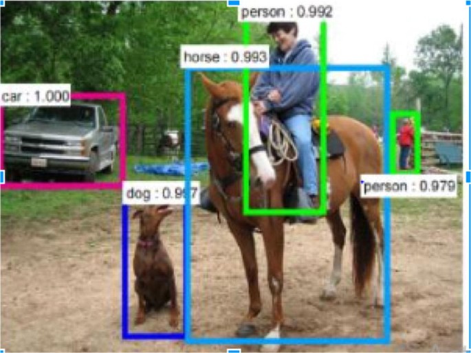
Detected objects using Keras RetinaNet
- Step 3:
-
For each keyframe KFi,j, four vectors are computed as follows:
-
1.
Occurrence Vector (OVi,j): It is a vector of dimension 80 that counts the number of objects of each of the 80 categories that has appeared in the keyframe KFi,j. For example, the vector for the frame in Fig. 2 will have a count equal to zero for all the object categories except for car, dog, horse and person. The count for the first three categories is 1, while for person is 2 (two persons are detected in the frame).
-
2.
Score Vector (SVi,j): Since each detected object has a score of detection, we compute a score vector of dimension 80 that contains the sum of scores of all the objects in the keyframe KFi,j. For example, the score value for the category person is 0.992 + 0.979 = 1.971, for the category car is 1, for the category horse is 0.993, and for the category dog is 0.997.
-
3.
Binary Vector (BVi,j): It is similar to the occurrence vector, but it computes a binary number instead of counting the number of times each of the 80 categories is detected in the key frame. In this case, the vector is an 80-dimensional one with zero values except for the categories: car, person, dog and horse, which are equal to 1.
-
4.
ConvPool Vector (ConvPVi,j): For each detected object O k i,j in KFi,j, we pass the englobing zone through a CNN network that generates a 128-dimensional vector named ConvPV k i,j . The network is composed of two sequential Conv2d layers followed by a max pooling layer and then two sequential Conv2d layers followed by an average pooling layer. The ConvPVi,j is calculated as follows:
$$ConvPV_{i,j} = \frac{1}{{NBO_{i,j} }}\mathop \sum \limits_{k = 1}^{{NBO_{i,j} }} ConvPV_{i,j}^{k},$$where NBOi,j is the number of detected objects in KFi,j
-
1.
- Step 4:
-
For each keyframe KFi,j, the above four vectors are concatenated into one matrix named DFFMi,j (deep features frame matrix) as follows:
$$DFFM_{i,j} = \left[ {\begin{array}{*{20}c} {OV_{i,j} } \\ {SV_{i,j} } \\ {BV_{i,j} } \\ {ConvPV_{i,j} } \\ \end{array} } \right]$$ - Step 5:
-
Each video Vi is represented by the set of DFFMi,j named DFVMi (deep features video matrix) of all its KFi,j as follows:
$$DFVM_{i} = \left[ {\begin{array}{*{20}c} {DFM_{i,1} } \\ {DFM_{i,2} } \\ \ldots \\ \ldots \\ {DFM_{{i,NBS_{i} }} } \\ \end{array}} \right]$$

3 Similarity between videos
In order to compute the similarity between two videos, we propose a two-step distance calculation.
Let us define first the distance between two keyframes KFi,l and KFj,m belonging to two videos Vi and Vj.
To compute the distance between two videos Vi and Vj based on the above-defined distance, we find the best k-matches between couple of keyframes Ki,l and Kj,m as follows:
To find the best k-matches in Mat, we proceed as follows:
Repeat k times:
- Step 1:
-
find the minimum in Mat and add it to the list of k-matches. Let it be d(KFi,l, KFj,m)
- Step 2:
-
eliminate from Mat all values d(KFi,o, KFj,p) with o = l or p = m
4 Experimentations and results
In order to test the efficiency of our video representation, we have conducted two types of experimentations. In the first type, we have clustered the set of videos in our dataset into several clusters using the k-medoid algorithm and based on the above-defined distance, and then, we have computed the mAP measure. In the second type, we have trained a model for each category using several classification methods, and then calculated several evaluation measures.
In our experimentations, we have used the dev part of the BlipTv dataset [17]. This dataset contains two sets of videos. The dev set contains 5288 videos in which we found 27 videos containing problems (empty, does not open, etc.), while the test set contains about 9000 videos. For each video, semi-professional user-generated (SPUG) content has been attached such as some metadata provided by the uploader, automatic speech recognition transcripts, automatic shot boundary files and social information. In our experimentations, we have based on the detected shots provided by the creators of the dataset. The shot boundary detection was performed using [20], and each shot was represented by its middle frame.
The videos of the dataset are categorized into 25 categories (Fig. 3). The category of a video is given by the user when uploading the video on the BlipTV website. Among the categories, we find the default category. This category contains all the videos that were not assigned a category by the uploader and all the other categories that contain less than 100 videos. In other words, this category may contain videos of different categories including the existing categories.

Genre distribution among categories in each set [17]
4.1 Video clustering
As mentioned above, we have applied the k-medoid algorithm with the above-defined distance (α1 = α2 = α3 = α4) on the set of 5261 videos with k = 25 (number of real categories). The mAP calculated on the clusters is 0.3379 which competes the results obtained by other works on the same dataset as we will show in the below discussion subsection.
4.2 Video classification
As presented before, a video is represented by the DFFM of all its keyframes. One problem we may face when using most of the classification approaches is that the DFVM of two videos may probably have different sizes. To avoid that, we have calculated the DFVM in the classification context as the average of the DFFMs of all its keyframes. In this case, the DFVM will be as follows:
Several classification methods have been tested. We have used 70% of the dev set for training and 30% of the dev set for testing. Using the random forest algorithm, the best results are obtained with an accuracy of 68.1% as shown in Table 1.
4.3 Discussion
The results obtained are compared to six works participated in the tagging task on this dataset (ARF [21], KIT [22], TUB [23], TUD [24], TUD_MM [25] and UNI_Camp [26]). These works are based on features extracted from one or more modalities. Table 2 shows the obtained results with a comparison against their results since they have used the same dataset.
As shown in the table, we have reached an accuracy of 68% in classification and a mAP of 33.8% in clustering using only visual features which are very competitive results. We had no chance to compare our work to deep learning video classification approaches since we do not have the same dataset. Even for the works that the datasets are available such as YouTube-1M and YouTube-8M, these datasets do not provide the raw videos but only features extracted from some frames inside the videos.
5 Conclusion
In this paper, we have proposed a new video representation technique for video classification and clustering aims named VideoToVecs. Most of the existing techniques focus on the extraction of features from the entire video frames. In contrast, we propose to extract features representing recognized objects inside the keyframes of the shots. We have then proposed a distance to compare the similarity between two videos. This similarity measure is used to cluster the videos into clusters in which the obtained results proved the efficiency of our proposal. Moreover, the classification results have shown that representing objects is efficient. The next step of our work is to enhance the representation with features derived from other sources such as speech transcript, social media and metadata.
References
Zhu W, Toklu, Liou S-P (2001) Automatic news video segmentation and categorization based on closed-captioned text. In: IEEE international conference on multimedia and expo (ICME2001), Tokyo, Japan
Roach M, Mason J (2001) Classification of video genre using audio. In: 7th European conference on speech communication and technology (Eurospeech), Aalborg, Denmark
Iyengar G, Lippman A (1997) Models for automatic classification of video sequences. In: Proceedings of SPIE storage and retrieval for image and video databases VI, CA, USA
Xu L-Q, Li Y (2003) Video classification using spatial-temporal features and PCA. In: Proceedings of the 2003 international conference on multimedia and expo (ICME2003), MD, USA
Ibrahim ZAA, Ferrane I, Joly P (2011) A similarity-based approach for audiovisual document classification using temporal relation analysis. EURASIP J Image Video Process 2011:537372. https://doi.org/10.1155/2011/537372
Ibrahim ZAA, Ferrane I, Joly P (2018) Temporal relation algebra for audiovisual data analysis. In: Furht B (ed) Multimedia tools and applications, multimedia tools and applications. Springer, Berlin. https://doi.org/10.1007/s11042-018-6771-1
Krizhevsky A, Sutskever I, Hinton G (2012) ImageNet classification with deep convolutional neural networks. Adv Neural Inf Process Syst 25(2):1097–1105. https://doi.org/10.1145/3065386
Simonyan K, Zisserman A (2015) Very deep convolutional networks for large-scale image recognition. In: International conference on learning representations, BC, Canada
Szegedy C, Liu W, Jia Y, Sermanet P, Reed S, Anguelov D, Erhan D, Vanhoucke V, Rabinovich A (2015) Going deeper with convolutions. In: IEEE conference on computer vision and pattern recognition (CVPR), MA, USA
He K, Zhang X, Ren S, Sun J (2016) Deep residual learning for image recognition. In: IEEE conference on computer vision and pattern recognition (CVPR), NV, USA
Deng J, Dong W, Socher R, Li L-J, Li K, Fei-Fei L (2009) ImageNet: a large-scale hierarchical image database. In: IEEE conference on computer vision and pattern recognition (CVPR), FL, USA
Sun J, Wang J, Yeh T-C (2017) Video understanding: from video classification to captioning. In: Stanford University. http://cs231n.stanford.edu/reports/2017/pdfs/709.pdf. Accessed Feb 2019
Zha S, Luisier F, Andrews W, Srivastava N, Salakhutdinov R (2015) Exploiting image-trained CNN architectures for unconstrained video classification. In: British machine vision conference (BMVC), Swansea, UK
Li F, Gan C, Liu X, Bian Y, Long X, Li Y, Li Z, Zhou J, Wen S (2017) Temporal modeling approaches for large-scale Youtube-8 M video understanding. In: Computing research repository. arXiv http://arxiv.org/abs/1707.04555
An E, Ji A, Ng E (2017) Large scale video classification using both visual and audio features on Youtube-8 M Dataset. In: Stanford University http://cs231n.stanford.edu/reports/2017/pdfs/702.pdf. Accessed Feb 2019
Simonyan K, Zisserman A (2014) Two streams convolution networks for action recognition in videos. In: Advances in neural information processing systems. http://arxiv.org/abs/1406.2199
Schmiedeke S, Xu P, Ferrané I, Eskevich M, Kofler C, Larson M, Estève Y, Lamel L, Jones G, Sikora T (2013) Blip10000: a social video dataset containing SPUG content for tagging and retrieval. In: ACM multimedia systems conference, Oslo, Norway
Lin T-Y, Goyal P, Girshick R, He K, Dollár P (2017) Focal loss for dense object detection. In: IEEE international conference on computer vision (ICCV), Venice, Italy
Lin T-Y, Maire M, Belongie S, Hays J, Perona P, Ramanan D, Dollár P, Zitnick L (2014) Microsoft COCO: common objects in context. In: European conference on computer vision, Zurich, Switzerland
Kelm P, Schmiedeke S, Sikora T (2009) Feature-based video key frame extraction for low quality video sequences. In: 10th workshop on image analysis for multimedia interactive services, London, UK
Ionescu B, Mironica I, Seyerlehner K, Knees P, Schluter J, Schedl M, Horia C, Buzo A, Lambert P (2012) ARF @ MediaEval 2012: multimodal video classification. In: Proceedings of the MediaEval 2012 Workshop, Pisa, Italy
Semela T, Tapaswi M, Ekenel HK, Stiefelhagen R (2012) KIT @ MediaEval 2012: content-based genre classification using visual cues. In: Proceedings of the MediaEval 2012 Workshop, Pisa, Italy
Schmiedeke S, Kelm P, Sikora T (2012) TUB @ MediaEval 2012 tagging task: feature selection methods for bag-of-(visual)-words approaches. In: Proceedings of the MediaEval 2012 Workshop, Pisa, Italy
Shi Y, Larson M, Wiggers P, Jonker C (2012) MediaEval 2012 tagging task: prediction based on one best list and confusion networks. In: Proceedings of the MediaEval 2012 Workshop, Pisa, Italy
Xu P, Shi Y, Larson M (2012) TUD @ MediaEval 2012 genre tagging task: multi-modality video categorization with one-vs-all classifiers. In: Proceedings of the MediaEval 2012 Workshop, Pisa, Italy
Almeida J, Salles T, Martins E, Penatti O, Torres R, Goncalves M, Almeida J (2012) UNICAMP-UFMG @ MediaEval 2012: genre tagging task. In: Proceedings of the MediaEval 2012 Workshop, Pisa, Italy
Author information
Authors and Affiliations
Corresponding author
Ethics declarations
Conflict of interest
On behalf of all authors, the corresponding author states that there is no conflict of interest.
Additional information
Publisher's Note
Springer Nature remains neutral with regard to jurisdictional claims in published maps and institutional affiliations.
Rights and permissions
About this article

Cite this article
Ibrahim, Z.A.A., Saab, M. & Sbeity, I. VideoToVecs: a new video representation based on deep learning techniques for video classification and clustering. SN Appl. Sci. 1, 560 (2019). https://doi.org/10.1007/s42452-019-0573-6
Received:
Accepted:
Published:
DOI: https://doi.org/10.1007/s42452-019-0573-6