Explicit realization of elements of the Tate–Shafarevich group constructed from Kolyvagin classes

Abstract

We consider the Kolyvagin cohomology classes, associated to an elliptic curve $E/{\mathbb Q}$, from a computational point of view. We explain how to go from a model of a class as an element of $(E(L)/pE(L))^{\mathrm {Gal}(L/{\mathbb Q})}$, where p is prime and L is a dihedral extension of ${\mathbb Q}$ of degree 2p, to a geometric model as a genus one curve embedded in $\mathbb { P} ^{p-1}$. We adapt the existing methods to compute Heegner points to our situation, and explicitly compute them as elements of E(L). Finally, we compute explicit equations for several genus one curves that represent non-trivial elements of , for $p \le 11$, and hence are counterexamples to the Hasse principle.

1 Introduction

Let $E/\mathbb {Q}$ be an elliptic curve of conductor N, with a fixed modular parametrization $\varphi : X_{0}(N) \xrightarrow {} E$. Let K be an imaginary quadratic field satisfying the Heegner hypothesis: all prime factors of N are unramified and split in K. Let H be the Hilbert class field of K. Using the theory of complex multiplication and the modular parametrization $\varphi$, one defines certain points in E(H), known as Heegner points.

Let us fix an odd prime p. Kolyvagin [18] has used Heegner points to construct certain elements of the p-Selmer group $\mathrm {Sel}^{(p)}(E/\mathbb { Q} )$. The images of these elements in the Tate–Shafarevich group , under the natural map , are known as Kolyvagin classes. It is a standard fact, due to Cassels [4], that elements of can be represented by genus one curves embedded in $\mathbb { P} ^{p-1}$.

The main result of this paper is an algorithm (divided into Algorithm 5.1 and Algorithm 3.2) to compute such representations for the Kolyvagin classes in , and thus obtain explicit counterexamples to the Hasse principle. In Sect. 6 we then use these algorithms to compute explicit equations for smooth genus one curves embedded in $\mathbb { P} ^{p-1}$, that have points over every completion of ${\mathbb Q}$, but no points defined over ${\mathbb Q}$ for primes $p \le 11$.

These calculations are especially interesting if $p>5$, and the curve E does not admit a p-isogeny. The standard method to compute such counter examples to the Hasse principle is to use the method of complete p-descent to compute the entire p-Selmer group $\mathrm {Sel}^{(p)}(E/{\mathbb Q})$. However, when $p>5$, this is not feasible in practice, as one runs into difficulties with computing class groups of very large number fields. Our method does not run into this problem, and in particular, in Sect. 6, Example 6.3, we compute the first known explicit realization of a non-trivial element of for an elliptic curve E that does not have a 7-isogeny.

These classes have already been studied from a computational point of view by Jetchev, Lauter and Stein in [17]. They are able to compute representations of these classes as elements of E(L)/pE(L), where L is a certain abelian extension of K. However, their aim is only to test whether these classes are non-zero, for which this representation is sufficient, whereas we compute explicit equations defining the corresponding homogeneous space.

The problem of computing these equations breaks up into two problems. First, given a suitable elliptic curve E, an imaginary quadratic field K and a prime p, we compute a Heegner point $x_K$, defined over a certain dihedral extension of $\mathbb { Q}$. Our method for doing this is Algorithm 3.2. To this point we associate a Kolyvagin class $c \in \mathrm {Sel}^{(p)}(E/\mathbb { Q} )$. Algorithm 5.1 then represents this class by a genus one curve $C \subset \mathbb { P} ^{p-1}$. The main difficulty in our computations is caused by the fact that typically the Heegner points $x_K$ have very large height, making them hard to compute and work with. We note that despite this, the output of Algorithm 5.1 is a model for the curve C with small integral coefficients, i.e. a minimized and reduced model, in the sense of [7].

2 Background on Kolyvagin classes and statement of results

In this section we review basic material from the theory of Heegner points. The main references are the articles of Gross, [15] and [14], as well as [24, 25] and Chapter 8 of [9].

2.1 Heegner points on modular curves

For $N \ge 1$ an integer, let $Y_0(N)$ be the open modular curve, defined over $\mathbb { Q}$. The $\mathbb { C}$-points of $Y_0(N)$ classify isomorphism classes of cyclic N-isogenies $E \xrightarrow {} E'$, defined over $\mathbb { C}$. Fix an imaginary quadratic field K satisfying the Heegner hypothesis: every prime dividing N splits completely in K. It follows that there exists an ideal $\mathcal { N}$ of the ring of integers $\mathcal { O} _K$ with $\mathcal { N} \bar{\mathcal { N} }=N \mathcal { O} _K$, and hence $\mathcal { O} _{K}/ \mathcal { N} \cong {\mathbb Z}/ N {\mathbb Z}$.

Given such an ideal $\mathcal { N}$, an ideal class $[\mathfrak {a}] \in \mathrm {Cl}(\mathcal { O} _K)$ determines a map of complex tori $\mathbb { C} /\mathfrak {a} \xrightarrow {} \mathbb { C} /\mathfrak {a}\mathcal { N} ^{-1}$. Since we have $\mathfrak {a}\mathcal { N} ^{-1}/\mathfrak {a} \cong \mathbb { Z} /N\mathbb { Z}$, this map is a cyclic N-isogeny, and determines a point in $Y_0(N)(\mathbb { C} )$. This is defined to be the Heegner point associated to the triple $x_K=(\mathcal { O} _K,[\mathfrak {a}],\mathcal { N} )$.

2.2 Rationality of Heegner points

A key property of Heegner points, implied by the theory of complex multiplication, is that they are defined over abelian extensions of the field K. More precisely, let $(\mathcal { O} _K,[\mathfrak {a}],\mathcal { N} )$ be a Heegner point on $Y_0(N)$. This point is defined over the Hilbert class field H of K. See $\S 5$ of [14]. The key point is that both $\mathbb { C} /\mathfrak {a}$ and $\mathbb { C} /\mathfrak {a}\mathcal { N} ^{-1}$ have complex multiplication by $\mathcal { O} _K$. This is a consequence of the Shimura reciprocity law, as explained in Chapter 6.8 of [21], or Chapter II of [22].

The field H is an abelian extension of K, and the Artin map provides a canonical isomorphism $F:\mathrm {Cl}(\mathcal { O} _K) \xrightarrow {} \mathrm {Gal}(H/K)$. Explicitly, by Shimura reciprocity, for an ideal class $[\mathfrak {b}]$ we have

$$\begin{aligned} (\mathcal { O} _K,[\mathfrak {a}],\mathcal { N} )^{F([\mathfrak {b}])}= (\mathcal { O} _K,[\mathfrak {ab^{-1}}],\mathcal { N} ). \end{aligned}$$

Suppose that $\tau \in \mathrm {Gal}(H/\mathbb { Q} )$ is a lift of complex conjugation. The action of $\tau$ is given by

$$\begin{aligned} (\mathcal { O} _K,[\mathfrak {a}],\mathcal { N} )^{\tau }=(\mathcal { O} _K,[\tau (\mathfrak {a})],\tau (\mathcal { N} )). \end{aligned}$$

2.3 Heegner points on elliptic curves and Kolyvagin classes

Now let E be an elliptic curve defined over $\mathbb { Q}$, of conductor N. Let $X_0(N)$ be the compactified modular curve of level N. By the modularity theorem (see [1]), there exists a modular parametrization map $\varphi : X_0(N) \xrightarrow {} E$. For every discriminant D that satisfies the Heegner condition, we fix an ideal $\mathcal { N}$ with $N \mathcal { O} _K=\mathcal { N} \bar{\mathcal { N} }$, and define the Heegner point $x_{K} \in E(H)$ by setting $x_K=\varphi (\mathcal { O} ,[\mathfrak {a}],\mathcal { N} )$. We also define the basic Heegner point $y_K \in E(K)$ by setting $y_K=\mathrm {Tr}_{H/K} x_K$.

Let $p>2$ be a prime such that E(H)[p] is trivial, $y_K \in pE(K)$ and p divides $|\mathrm {Cl}(\mathcal { O} _K)|=|H:K|$ exactly once. These assumptions are fairly mild, as we will see later. Then there exists a unique degree p subfield of H, which we denote by L. Let $z_{K}=\mathrm {Tr}_{H/L} x_{K}$, and let $\sigma$ be a generator of $G=\mathrm {Gal}(L/K).$ Define the operators $D_{\sigma }$ and $\mathrm {Tr}$ in $\mathbb {Z}[G]$ by

$$\begin{aligned} D_{\sigma }=\sum _{i=1}^{p-1} i \sigma ^i, \quad \mathrm {Tr}=\sum ^{p-1}_{i=0} \sigma ^i. \end{aligned}$$

The operator $D_{\sigma }$ is known as the Kolyvagin derivative and $\mathrm {Tr}$ is the trace operator. They satisfy the identity

$$\begin{aligned} (\sigma -1)D_{\sigma }=p-\mathrm {Tr}, \end{aligned}$$

We define the derived Heegner point P as $P=D_{\sigma } \cdot z_K$. The class $[P] \in E(L)/pE(L)$ is invariant under the action of G, since we have

$$\begin{aligned} (\sigma -1)(D_{\sigma } \cdot z_K)=p z_K- \mathrm {Tr} (z_K)=p z_K-\mathrm {Tr}_{H/K} (x_K)=p z_K-y_K, \end{aligned}$$

and by assumption $y_K \in pE(K)$. The Kummer map $\delta : E(L)/p(L) \xrightarrow {} H^1(L,E[p])$ is compatible with the Galois action, and so we can define a cohomology class $c_L \in H^1(L,E[p])^{\mathrm {Gal}(L/K)}$ by $c_L=\delta ([P])$. We have the inflation-restriction exact sequence

$$\begin{aligned} H^1(L/K, E[p](L)) \xrightarrow {\mathrm {inf}} H^1(K,E[p]) \xrightarrow {\mathrm {res}} H^1(L,E[p])^{\mathrm {Gal}(L/K)} \xrightarrow {} H^2(L/K, E[p](L)). \end{aligned}$$

As E[p](L) is trivial, the two outermost groups are trivial, and the restriction map defines an isomorphism $\mathrm {res}: H^1(K,E[p]) \xrightarrow {} H^1(L,E[p])^{\mathrm {Gal}(L/K)}$. We define $c \in H^1(K,E[p])$ to be the preimage of $c_L$ under the restriction map. The class c is in fact an element of the p-Selmer group $\mathrm {Sel}^{(p)}(E/K)$, see [15, Prop 6.2]. Finally, let d be the image of c in $H^1(K,E)$. Then d is an element of .

Remark 2.1

The above definition is less general than the one Kolyvagin used—he also used Heegner points defined over ring class fields to define Kolyvagin classes. Our method extends to these classes as well with minor changes, but to make exposition simpler we restrict to the case when the Heegner point is defined over the Hilbert class field. In practice, when computing examples with $p\ge 7$, these points appear to be easier to compute.

2.4 Descent from K to $\mathbb { Q}$

Let $\epsilon$ be the sign of the functional equation of $E/\mathbb {Q}$. The proof of Proposition 5.4 in [15] shows that the class c lies in the $\epsilon$-eigenspace for the action of complex conjugation on $H^1(K,E[p])$. Thus, if E is a curve of rank 0, c is fixed by complex conjugation, and by the same inflation-restriction argument we naturally obtain an element of $H^1(\mathbb {Q},E[p])$, which we will also call c.

As E has no non-trivial p-torsion and rank 0, the group $E(\mathbb {Q})/pE(\mathbb {Q})$ is trivial, and hence if c is non-zero, its image d in $H^1(K,E[p])$ will be a non-trivial element of . Tracing through the isomorphisms used to define c, we see that the class c is non-zero if and only if the point P is not divisible by p in E(L).

2.5 Galois cohomology and n-diagrams

Let F be a number field, E/F an elliptic curve and $n \ge 1$ an integer. We briefly recall a few standard facts about the Galois cohomology groups $H^1(F,E)$ and $H^1(F,E[n])$, see for example [5].

A torsor under E is a smooth projective curve T/F, together with a regular simply transitive action of E on T, defined by a morphism $E \times T \xrightarrow {} T$. An isomorphism of torsors $C_1$ and $C_2$ is an isomorphism of curves $C_1$ and $C_2$ that respects the action of E. The left action of E on itself by translations makes E a torsor, which we call the trivial torsor. There is a natural identification of the group $H^1(F,E)$ with the set of isomorphism classes of torsors defined over F, and the trivial torsor E corresponds to the identity element.

We will also need the following interpretation of the group $H^1(F,E[n])$. We define a diagram $[C \xrightarrow []{} S]$ to be a morphism from a torsor C to a variety S. An isomorphism of diagrams $[C_1 \xrightarrow {} S_1] \sim [C_2 \xrightarrow {} S_2]$ is an isomorphism of torsors $\varphi : C_1 \cong C_2$ together with an isomorphism of varieties $\psi : S_1 \cong S_2$ making the diagram

commute. We define the trivial n-diagram to be the diagram $[E \xrightarrow []{} \mathbb { P} ^{n-1}]$ where the morphism is induced by the complete linear system of the divisor $n \cdot 0_E$, and in general, we say a diagram $[C \xrightarrow []{} S]$ is an n-diagram if it is defined over F, but isomorphic to the trivial diagram over the algebraic closure $\bar{F}$, i.e. a twist of the trivial diagram. The set of isomorphism classes is also naturally identified with $H^1(F,E[n])$.

The group law on E induces a summation map $\mathrm {sum} : \mathrm {Div} E \xrightarrow []{} E$, given by $\sum n_p \cdot (P) \mapsto \sum n_pP.$ Two divisors D and $D'$ of the same degree are linearly equivalent if and only $\mathrm {sum}(D)=\mathrm {sum}(D')$. The Kummer map $\delta : E(F)/nE(F) \xrightarrow {}H^1(F,E[n])$ sends a class $[P] \in E(F)/nE(F)$ to the isomorphism class of the n-diagram $[E \xrightarrow []{} \mathbb { P} ^{n-1}]$, where the map is induced by the complete linear system of any degree n divisor D with $\mathrm {sum}(D)=P$.

In this article we consider only n-diagrams of the form $[C \xrightarrow []{} {\mathbb P}^{n-1}]$. When $n \ge 3$, such an n-diagram is a closed embedding, and its image is a smooth projectively normal curve C of genus one and degree n. If $n=3$, C is a plane cubic. For $n \ge 4$, the ideal defining C is generated by $n(n-3)/2$ quadrics, see [10, Prop. 5.3]. Finally, as a consequence of class field theory, under the above identification, the elements of the n-Selmer group of E can be represented by n-diagrams of the form $[C \xrightarrow []{} \mathbb { P} ^{n-1}]$.

2.6 Summary of the setup and the statement of results

Our starting data is an elliptic curve $E/{\mathbb Q}$ of rank 0 and an odd prime p for which the Birch and Swinnerton-Dyer conjecture predicts that the group is non-trivial. To construct a Kolyvagin class, we also need to find a discriminant D of an imaginary quadratic field K with Hilbert class field H that satisfies the following: D satisfies the Heegner hypothesis, E(H)[p] is trivial, p divides $|\mathrm {Cl}(\mathcal { O} _K)|=|H:K|$ exactly once, the rank of E/K is 0, and the basic Heegner point $y_K$ is divisible by p in E(K).

Remark 2.2

For given E and p, it is usually easy to find a discriminant D that satisfies these conditions. In practice, a naive search will usually find plenty of discriminants that are easily seen to satisfy all conditions but the last one, and a famous theorem of Kolyvagin (Theorem 1.3 of [15]) then often guarantees that we must have $p|y_K$.

Starting from the data of E, p and D, we compute a p-diagram representing the Kolyvagin class $c \in \mathrm {Sel}^{(p)}(E/{\mathbb Q})$ defined above. There are two main steps. Algorithm 3.2 computes the Heegner point $x_K$ as an element of E(H), and using this data Algorithm 5.1 then computes the equations defining a genus one normal curve $C \subset \mathbb { P} ^{p-1}$, and the inclusion $C \subset \mathbb { P} ^{p-1}$ is the p-diagram representing the class c. If this class is non-trival, the curve C is a counter-example to the Hasse principle. We are able to succesfully use these algorithms for various elliptic curves with $p=3,5$ and 7, and we give examples in Sect. 6. Note that the examples with $p=3$ and $p=5$ can also be obtained by the method of p-descent, but Example 6.3 with $p=7$ is out of reach of p-descent at the moment, and is the first such example with no 7-isogeny to our knowledge.

Remark 2.3

If the curve E has rank 1 over ${\mathbb Q}$, then the class d is in the $(-1)$-eigenspace of complex conjugation, and hence is obtained as the restriction of an element of , where $E_D$ is the quadratic twist of E by D. If this quadratic twist has rank 0, then by the same argument, the class d is non-zero if and only if the class c is.

Our method applies in this case as well, and in fact we are able to compute an example (Example 6.5) with $p=11$, i.e. a genus one normal curve $C \subset \mathbb { P} ^{10}$ that is a counter-example to the Hasse principle. We suspect that p could be increased even further, since computing the Heegner point appears to be much easier in this case. As the Kolyvagin class is naturally an element of for the quadratic twist $E_D$ of the curve E we begin with, it seems difficult to use this version of our method as a tool to compute of a given curve E.

3 Computing the Heegner point

In this section we describe the algorithm we will use to compute the Heegner points needed to define the Kolyvagin class.

3.1 Computing the modular parametrization

We briefly recall how to compute a modular parametrization of an elliptic curve, following [9] and [17]. Let $E/\mathbb {Q}$ be an elliptic curve of conductor N, p an odd prime, and let K be an imaginary quadratic field. We assume that the maximal order $\mathcal { O} _K$ of K is of discriminant $-D\ne 3,4$ and that K satisfies the Heegner hypothesis: all prime factors of N split completely in $\mathcal { O} _K$. We fix an ideal $\mathcal { N}$ with $N \mathcal { O} _K= \mathcal { N} \bar{\mathcal { N} }$. Let H be the Hilbert class field of K, and fix a modular parametrization $\varphi : X_0(N) \xrightarrow {} E$ that maps the cusp $\infty$ to the origin of E. We assume that H has unique subfield of degree p over K, denoted L. The Heegner point $x_K$ is defined to be the image $x_K=\varphi (\mathcal { O} _K,[\mathcal { O} _K],\mathcal { N} ) \in E(H)$, and we set $z_{K}=\mathrm {Tr}_{H/L} x_{K}$.

Following [17], we give an explicit description of the map $\varphi$. Let $\Lambda$ be the period lattice associated to E, and let $f\in S_2(\Gamma _0(N))$ be the newform associated to E. Let $\mathcal { H} ^{*}=\mathcal { H} \cup \mathbb {Q} \cup \{\infty \}$ be the extended upper half plane, and identify the modular curve $X_0(N)$ with the quotient $\mathcal { H} ^*/\Gamma _0(N)$. The modular parametrization map $\varphi :X_0(N) \xrightarrow {} \mathbb {C}/\Lambda$ is given by integrating the holomorphic differential f(z)dz on $X_0(N)$. We can compute it using the power series

$$\begin{aligned} \varphi (\tau )=\int ^{\infty }_{\tau } f(z)dz=\sum _{n \ge 1} \frac{a_n}{n} e^{2\pi i n \tau }, \end{aligned}$$

(1)

where $f=\sum _{n\ge 1}a_n q^n$ is the Fourier expansion of f. To obtain a parametrization $X_0(N) \xrightarrow {} E$, we compose with the uniformization $\psi :\mathbb {C}/\Lambda \xrightarrow {} E(\mathbb { C} )$. The map $\psi$ is defined using the Weierstrass $\wp$-function, and is easy to compute numerically to high precision.

The Artin map provides us with an isomorphism between the class group $\mathrm {Cl}(\mathcal { O} _K)$ and the Galois group $\mathrm {Gal}(H/K)$. We first compute a set of representatives $\mathfrak {a}_1,\ldots ,\mathfrak {a}_m$ for $\mathrm {Cl}(\mathcal { O} _K)$. Let $\sigma _i$ be the image of $\mathfrak {a}_i$ under the Artin map. The Galois conjugates of the point x corresponding to the isogeny $[\mathbb {C}/\mathcal {O}_{K} \xrightarrow {} \mathbb {C}/\mathcal {N}^{-1}]$ are given by

$$\begin{aligned} \sigma _i(x)= [\mathbb {C}/\mathfrak {a}^{-1}_i \xrightarrow {} \mathbb {C}/\mathfrak {a}^{-1}_i \mathcal {N}^{-1}]. \end{aligned}$$

(2)

For every conjugate we compute a corresponding point $\tau$ in the upper half plane. Fix an embedding $\iota$ of L into $\mathbb {C}$. As the morphism $\varphi$ is defined over $\mathbb {Q}$, we can use the above description of the Galois action to compute the coordinates of the Galois conjugates $\sigma _i(x_K)$, to whatever precision we like. We then to do same for the point $z_K=\mathrm {Tr}_{H/L}(x_K)$. By assumption, L is the unique degree p subfield of H, and so it is the fixed field of the unique index p subgroup of $\mathrm {Gal}(H/K)$. We enumerate the corresponding elements $[\mathfrak {a}_{i_1}],[\mathfrak {a}_{i_2}],\ldots ,[\mathfrak {a}_{i_{m/p}}]$ of $\mathrm {Cl}(\mathcal { O} _K)$ and then compute $z_K$ numerically from the sum $z_K=\sum _{j=1}^{m/p} \sigma _{i_j}(x_K)$.

3.2 Recognizing the Heegner point using lattice reduction

We now discuss how to use the LLL algorithm to recover the point $z_K$ from the data computed in the previous section. Recognizing an algebraic number from floating point approximations is a well-studied problem, and in the setting of Heegner points has been considered in [17]. An algorithm similar to the one they propose has been implemented in MAGMA by Steve Donnelly. For our purposes however, their method is too slow to handle the case when $p \ge 5$, so in this section we propose a variant to this method that seems to work quite well in this setting.

Let L be a number field of degree n, with n complex embeddings $\sigma _1,\ldots ,\sigma _{n}$, and let $\alpha _1,\ldots ,\alpha _{n}$ be a ${\mathbb Z}$-basis of the ring integers $\mathcal {O}_{L}$. In our application L will be a dihedral extension of ${\mathbb Q}$ of degree 2p.

Definition 3.1

Let $\epsilon >0$, $C=10^B$ for an integer $B>0$, $z \in L$ and let $z_1,\ldots ,z_{n} \in \mathbb {C}$ be such that $|\sigma _i(z) -z_i|~ <\epsilon$. Let $\alpha _{ij} \in \mathbb {C}$ be such that $|\sigma _j(\alpha _i)-\alpha _{ij}|<\epsilon$. To this data we associate the $2n\times 3n$ integer matrix $A_{z,\epsilon ,C}$:

$$\begin{aligned} \begin{pmatrix} 1 &{}\quad 0 &{}\quad \ldots &{}\quad 0 &{} 0 &{} \lfloor {C\alpha _{1,1}}\rfloor &{}\ldots &{} \lfloor {C\alpha _{1,n}}\rfloor \\ \vdots &{}\quad \vdots &{}\quad \ddots &{}\quad \vdots &{} \vdots &{} \vdots &{}\ldots &{} \vdots \\ \vdots &{}\quad \vdots &{} \quad \ldots &{}\quad \vdots &{} \vdots &{} \lfloor {C\alpha _{n,1}}\rfloor &{}\ldots &{}\lfloor {C\alpha _{n,n}}\rfloor \\ \vdots &{}\quad \vdots &{}\quad \ldots &{}\quad \vdots &{} \vdots &{} \lfloor {C\alpha _{1,1} z_1}\rfloor &{}\ldots &{}\lfloor {C\alpha _{1,n} z_{n}}\rfloor \\ \vdots &{}\quad \vdots &{}\quad \ddots &{}\quad \vdots &{} \vdots &{} \vdots &{} \vdots &{}\vdots \\ 0 &{}\quad 0 &{}\quad \ldots &{} \quad 0 &{}\quad 1 &{}\lfloor {C \alpha _{n,1} z_1}\rfloor &{} \ldots &{}\lfloor {C\alpha _{n,n} z_{n}}\rfloor \end{pmatrix} \end{aligned}$$

i.e. the left $2n\times 2n$-block is the $2n\times 2n$ identity matrix, and the right $2n\times n$-block splits into the upper $n \times n$-block $(\lfloor {C\alpha _{ij}}\rfloor )_{ij}$ and the lower $n \times n$-block $(\lfloor {C\alpha _{ij} z_j}\rfloor )_{ij}$. We define $L_{z,\epsilon ,C}$ to be the lattice in $\mathbb {R}^{3n}$ spanned by the rows of $A_{z,\epsilon ,C}$.

We now explain the heuristic behind our algorithm to recover z from its numerical approximations. It is based on a standard idea used in algorithms to detect integer relations, see [16]. We look for integers $u_1,\ldots ,u_{2n}$ for which we have

$$\begin{aligned} 0=u_1\alpha _1+u_2\alpha _2+\ldots +u_n \alpha _{n}+u_{n+1}\alpha _{1}z+u_{n+2}\alpha _{2}z+\ldots +u_{2n}\alpha _{n}z. \end{aligned}$$

(3)

Such a set of integers certainly exists, since (3) is equivalent to

$$\begin{aligned} z=-\frac{\sum ^{n}_{i=1} u_i \alpha _i}{\sum ^{n}_{i=1} u_{n+i} \alpha _i}, \end{aligned}$$

allowing us to recover z. Let $r_1,\ldots ,r_{2n}$ denote the rows of $A_{z,\epsilon ,C}$, and consider the vector row vector $u_1r_1+\ldots +u_{2n}r_n$. The entries of this vector are

$$\begin{aligned} (u_1, u_2,\ldots ,u_{2n},\sum ^{n}_{i=1} (\lfloor {C\alpha _{i,1}}\rfloor +\lfloor {C\alpha _{i,1}z_1}\rfloor ) ,\ldots ,\sum ^{n}_{i=1}( \lfloor {C\alpha _{i,n}}\rfloor +\lfloor {C\alpha _{i,n}z_n}\rfloor )) \end{aligned}$$

and so if $\epsilon$ is small and C is large, the last n entries should be very small. If the integers $u_1,\ldots ,u_{2n}$ are chosen to be the smallest possible so that the relation (3) holds, then $u_1r_1+\ldots +u_{2n}r_n$ is a candidate for the shortest vector in the lattice $L_{z,\epsilon ,C}$. Thus we use the LLL algorithm to find the shortest vector in this lattice and hope that it actually corresponds to a relation (3). If it does not, we decrease $\epsilon$, increase C and try again. Note that we have not proven that this algorithm terminates, i.e. that for small enough $\epsilon$ the shortest vector corresponds to a relation (3), but as we were able to compute some very large examples with this method, it seems plausible that this is the case.

We summarise the discussion of this section in the following algorithm.

Algorithm 3.2

• INPUT: An elliptic curve E, a Heegner discriminant D, and a prime p that divides $|\mathrm {Cl}(\mathcal { O} _K)|$ exactly once.

• OUTPUT: Coordinates (x, y) of a point $P \in E(L)$ that is (conjecturally) the point $z_K=\mathrm {Tr}_{H/L}x_K$.

• (i) Find a set of representatives $\mathfrak {a}_1,\mathfrak {a}_2,\ldots ,\mathfrak {a}_{n}$ for the class group $\mathrm {Cl}(O_K)$, and for each point $[\mathbb {C}/\mathfrak {a}^{-1}_i \xrightarrow {} \mathbb {C}/\mathfrak {a}^{-1}_i \mathcal {N}^{-1}]$, compute a corresponding $\tau _i$ in the upper half plane.

• (ii) Compute an equation for the unique degree p subfield L of the Hilbert class field, and compute an integral basis of the maximal order $\mathcal {O}_{L}$.

• (iii) Pick an $\epsilon >0$, and compute $\varphi (\tau _i) \in \mathbb {C}$ to precision $\epsilon /2$, using the formula (1), by computing enough of the Fourier coefficients $a_n$.

• (iv) Compute the period lattice $\Lambda$ and hence the uniformisation map $\psi :\mathbb {C}/\Lambda \xrightarrow []{} E$ to the required precision, and hence find $\psi (\varphi (\tau _i))$. Then, use the description of the Galois action on Heegner points given in Sect. 2.2 to take the trace from H to L, and hence obtain $z_1,\ldots ,z_{2p}$ with $|\sigma _i(x)-z_i|<\epsilon$.

• (v) Using $z_1,z_2,\ldots ,z_{2p}$ and choosing a large constant C, form the matrix $A_{z,\epsilon ,C}$ as in Definition 3.1. Use the LLL algorithm to find a $U\in \mathrm {GL}_{4p}(\mathbb {Z})$ such that the rows of $UA_{z,\epsilon ,C}$ form an LLL-reduced basis of $L_{z,\epsilon ,C}$. Then let $x=-\frac{\sum ^{2p}_{i=1} u_{1,i} \alpha _i}{\sum ^{2p}_{i=1} u_{1,2p+i} \alpha _i}$ and test if x is the x-coordinate of a point in E(L). If it is, solve for the y-coordinate and return (x, y). Otherwise, replace $\epsilon$ by $\epsilon /2$, and return to Step 3.

Steps (i), (ii) and (iii) of the algorithm have been studied extensively in the literature, see for example Section 8.6 of [9] or [24], so we do not provide details on how to implement them. We have used the existing MAGMA implementations of these steps in our calculations. The algorithm has not proven that the point (x, y) is indeed the point $x_K$, although we believe it is highly probable that it is, nor have we proven that the algorithm always terminates. However, in practice we have been able to use it to compute points on various elliptic curves for $p\le 11$.

The main bottleneck is Step (iii). If the height of the Heegner point is very large, then we need to take $\epsilon$ to be very small for the algorithm to return a point in E(L), and this requires computing a very large number of the Fourier coefficients $a_n$.

Remark 3.3

The output of our algorithm, if it terminates, will be a point $u=(x',y') \in E(H)$, and as noted in [17], verifying that this point coincides with the Heegner point $z_K=(x,y)$ is a nontrivial matter. We know that the point we obtain is a good archimedean approximation of the Heegner point, in the sense that by increasing the precision in Algorithm 3.2 we can make the absolute values $|\sigma (x)-\sigma (x')|$, where $\sigma$ is any embedding $L \hookrightarrow \mathbb { C}$, as small as we like. However, without a bound on the height of $z_K$, we can’t actually prove that $u=z_K$.

Since our main goal is to construct examples of non-trivial elements of the Tate–Shafarevich group of E, it suffices to verify that the point u satisfies the same properties as the Heegner point $z_K$ for the purpose of constructing a Kolyvagin class, as formalized in Lemma 4.2. This also serves as a consistency check on our calculations, and in all of the examples we have computed, we believe it is very unlikely that the resulting point is not the Heegner point. Note that the appendix of [17] provides a method one could use to compute a bound on the height of $z_K$ and hence make the calculations provably correct, but we did not implement this algorithm.

Remark 3.4

The idea to use the LLL-algorithm method to recover z from the matrix $A_{z,\epsilon ,C}$ is very well known. Our approach differs from the standard method explained in Chapter 7 of [16]. Briefly, the standard method to recover an algebraic number z from a set of complex numbers $\{z_g : g \in G\}$ that approximate the Galois conjugates of z is to approximate the minimal polynomial f of z by $\prod _{g \in G}(x-z_g)$, and try to recognize the coefficients of f as rationals, using continued fractions, or better yet the LLL algorithm. However, for us this method is not efficient enough, since z is of very large height in the examples we consider, and the coefficients of the polynomial f are symmetric polynomials in $z_g$, and hence are of even larger height.

Our method instead tries to recognize z directly, taking advantage of the fact that we know that x is defined over the Hilbert class field H. We can compute this field beforehand, using the machinery of computational class field theory already implemented in MAGMA.

Remark 3.5

A further improvement along the same lines is to use the fact that we can also compute numerically the y-coordinate, and look for linear relations of the form $A+Bx+Cy=0$. Recall that we have assumed that L is of class number 1, so that $x=r/t^2$ and $y=s/t^3$, for some $r,s,t \in \mathcal { O} _L$. Thus if $A+Bx+Cy=0$, we see that t|A, and that hence $A^2x \in \mathcal { O} _L$. It is then simple to recover $A^2x$ from its floating point approximation, and hence to compute the point (x, y). Based on experimental data we have computed, this seems to be an improvement. A heuristic explanation might be that the minimal A, B, C that can appear in a relation $A+Bx+Cy=0$ can be a lot smaller than the minimal u, v appearing in a relation $u+vx=0$, and so it is easier to guess a short vector in the corresponding lattice.

4 Geometric realization of the Kolyvagin class

4.1 The p-diagram associated to the Kolyvagin class

In this section we explain how to compute, given a Heegner point, equations for the p-diagram representing the Kolyvagin class. The first step is to formalize the input we need from Heegner points to define Kolyvagin classes. After that, we first represent the Kolyvagin class by a p-diagram $C \subset PP^{p-1}$ defined over a dihedral extension $L/{\mathbb Q}$ of degree 2p, and give explicit formulas for the action of the Galois group $\mathrm {Gal}(L/{\mathbb Q})$ on $C \subset {\mathbb P}^{p-1}$. This action is encoded in a cocycle in $Z^1(\mathrm {Gal}(L/{\mathbb Q}),\mathrm {GL}_p(L))$. We then use Galois descent to reduce the problem of computing a p-diagram defined over ${\mathbb Q}$ that represents the Kolyvagin class to linear algebra.

Throughout this section, we fix the following data. Let $E/\mathbb {Q}$ be an elliptic curve of rank 0, let p be an odd prime and $K/\mathbb {Q}$ be a quadratic field. In addition, let $L/\mathbb { Q}$ be a dihedral extension, of degree 2p, that contains K, such that E(L)[p] is trivial.

Proposition 4.1

Let $P \in E(L)$ be a point such that the class $[P]\in E(L)/pE(L)$ is invariant under the action of $G=\mathrm {Gal}(L/\mathbb { Q} )$. Let $\delta :E(L)/pE(L) \xrightarrow {} H^1(L,E[p])$ be the Kummer map, and let $\mathrm {res} : H^1(\mathbb { Q} ,E[p]) \xrightarrow {} H^1(L,E[p])$ be the restriction map.

Then there exists a unique class $c \in H^1(\mathbb {Q},E[p])$ such that $\mathrm {res}(c)=\delta ([P])$.

Proof

This is the inflation-restriction argument from Sect. 2. $\square$

The aim of this section is to give method to compute equations for the p-diagram representing the class c. This is accomplished by Galois descent, and involves explicit cocycle calculations. Let $\sigma \in G$ be an element of order p, and let $\tau \in G$ be an involution.

Lemma 4.2

Let $P \in E(L)$ be a point with $[P] \in (E(L)/pE(L))^{G}$, and suppose that we also have $\tau (P)=P$. We then have the following.

• (i) For each $g \in G$, there exists a unique $R_g \in E(L)$ with $pR_g=g(P)-P$. The map $g \mapsto R_g$ defines a cocycle in $H^1(G,E(L))$, meaning that for any $g,h \in G$ we have

  $$\begin{aligned} R_{gh}=g(R_h)+R_g, \end{aligned}$$

• (ii) For $0 \le k \le p-1$, we have $R_{\sigma ^k}=\sum ^{k}_{i=1} \sigma ^{i-1}(R_{\sigma })$, and $R_{\sigma ^k\tau }=R_{\sigma ^k}$.

• (iii) We have $\sum ^{p}_{k=1} \sigma ^k (R_{\sigma })=0_E$ and $\tau (R_{\sigma ^k})=R_{\sigma ^{p-k}}$.

• (iv) We have $[P]=[D_{\sigma } R_{\sigma }]=[\sum ^{p-1}_{i=1} i\sigma ^i (R_{\sigma })]=[\sum ^{p-1}_{i=1} R_{\sigma ^i}] \in E(L)/pE(L)$.

Proof

• (i) Since $[g(P)]=[P]$ as elements of E(L)/pE(L) for every $g \in G$, there exists a point $R_{g}\in E(L)$ with $pR_g=g(P)-P$. As E(L)[p] is trivial, $R_g$ is unique and the cocycle condition follows from

  $$\begin{aligned} pR_{gh}=gh(P)-P=g(h(P)-P)+g(P)-P=pg(R_h)+pR_{g}=p(g(R_h)+R_g), \end{aligned}$$

• (ii) As $pR_{\sigma ^k \tau }=\sigma ^k\tau (P)-P=\sigma ^k(P)-P=pR_{\sigma ^k}$, we have $R_{\sigma ^k\tau }=R_{\sigma ^k}$. By (i) we have $R_{\sigma ^k}=\sigma (R_{\sigma ^{k-1}})+R_{\sigma }$, so we are done by induction on k.

• (iii) By (ii), $0_E=R_{\sigma ^p}=\sum ^{p}_{k=1} \sigma ^k (R_{\sigma })$. Using the identity $\sigma ^{p-k}\tau =\tau \sigma ^k$, we compute

  $$\begin{aligned} p \cdot \tau (R_{\sigma ^k})=\tau ( p \cdot R_{\sigma ^k}) = \tau \sigma ^k (P)- \tau (P)=\sigma ^{p-k}\tau (P)-P=p \cdot R_{\sigma ^{p-k}\tau } \end{aligned}$$

  and as before we conclude $\tau (R_{\sigma ^k})=R_{\sigma ^{p-k}\tau }$.

• (iv) Using (ii) we see that

  $$\begin{aligned} \sum ^{p-1}_{i=1} R_{\sigma ^i}=\sum ^{p-1}_{i=1}\sum ^{i}_{j=1} \sigma ^{j-1}(R_{\sigma })=\sum ^{p-1}_{i=1} i\sigma ^i (R_{\sigma })= D_{\sigma }R_{\sigma }. \end{aligned}$$

  By the identity $(\sigma -1) \cdot D_{\sigma }=p-\sum ^{p}_{i=1} \sigma ^i$ and (iii), we have

  $$\begin{aligned} \sigma (D_{\sigma }R_{\sigma })-D_{\sigma }R_{\sigma }=pR_{\sigma }-\sum ^{p}_{i=1} \sigma ^i( R_{\sigma })=pR_{\sigma }. \end{aligned}$$

  Using (iii), we find that $\tau (D_{\sigma }R_{\sigma })=\tau (\sum _{i=1}^{p} R_{\sigma ^i})=\sum _{i=1}^{p} R_{\sigma ^{p-i}}=D_{\sigma }R_{\sigma }$. Let $Q=P-D_{\sigma }R_{\sigma }$. We have $\sigma (D_{\sigma }R_{\sigma })-D_{\sigma }R_{\sigma }=\sigma (P)-P=pR_{\sigma }$, and hence $\sigma (Q)=Q$. Since $\tau (D_{\sigma }R_{\sigma })=D_{\sigma } R_{\sigma }$ and $\tau (P)=P$, we also have $\tau (Q)=Q$. As $\sigma$ and $\tau$ generate G, we have $Q \in E(\mathbb {Q})$. But we have assumed that $E(\mathbb {Q})$ is finite, so Q is a torsion point. As E(L)[p] is trivial, the image of Q in E(L)/pE(L) is zero, and hence $[P]=[D_{\sigma }R_{\sigma }]$, as desired.

$\square$

We now describe the p-diagram corresponding to $c_L$ and the action of the Galois group on this diagram. For a point $Q \in E(L)$, let $\varphi _{Q} : E \xrightarrow []{} E$ be the translation by Q morphism.

Proposition 4.3

• (i) Consider the degree p divisor D on E/L defined by $D=\sum ^{p}_{i=1} R_{\sigma ^i}$. Let $l_1,\ldots ,l_p$ be a basis of the Riemann-Roch space $\mathcal {L}(D)$ and let $E \xrightarrow {l} \mathbb {P}^{p-1}$ be the embedding induced by this choice of basis. Then $[E \xrightarrow {l} \mathbb {P}^{p-1}]$ is the p-diagram representing $c_L \in H^1(L,E[p])$.

• (ii) The action of the Galois group G on the divisor D is given by

  $$\begin{aligned} g\left( \sum _{i=0}^{p-1} R_{\sigma ^i}\right) =\varphi _{R_g}^{*}\left( \sum _{i=0}^{p-1} R_{\sigma ^i}\right) . \end{aligned}$$

• (iii) For each $g\in G$, the translation map $\varphi _{R_g}$ induces an isomorphism of p-diagrams $g \cdot [E \xrightarrow { l} \mathbb {P}^{p-1}]$ and $[E \xrightarrow {l} \mathbb {P}^{p-1}]$, represented by the commutative diagram

  

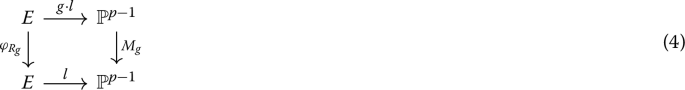
  where $M_g \in \mathrm {PGL}_p(L)$. The map $g \mapsto M_g$ determines a cocycle class in $H^1(G,\mathrm {PGL}_p(L))$.

Proof

By Lemma 4.2(iv), we have $[\mathrm {sum}(D)]=[D_{\sigma } R_{\sigma }]=[P] \in E(L)/pE(L)$, where $\mathrm {sum} : \mathrm {Div}(E) \xrightarrow {} E$ is the map adding up points on a divisor using the group law. Part (i) follows from the description of the Kummer map given in Sect. 2.4. For part (ii), by Lemma 4.2(ii) and (iii), we have $\sigma (R_{\sigma }^{i})=R_{\sigma ^{i}}-R_{\sigma }$ and $\tau (R_{\sigma ^{i}})=R_{\sigma ^{p-i}}$. From these identities we obtain

$$\begin{aligned} \sigma \left( \sum _{i=0}^{p-1} R_{\sigma ^i}\right) =\varphi _{R_{\sigma }}^{*}\left( \sum _{i=0}^{p-1} R_{\sigma ^i} \right) , \quad \tau \left( \sum _{i=0}^{p-1} R_{\sigma ^i}\right) =\sum _{i=0}^{p-1} R_{\sigma ^i}. \end{aligned}$$

The cocycle condition for $g \mapsto R_g$ implies the result for all $g \in G$.

To see the isomorphism of p-diagrams in (iii), note that by (ii) we have $\varphi ^{*}_{-R_g}(D)=g(D)$, and that $g(l_1),\ldots ,g(l_p)$ and $\varphi ^{*}_{-R_g}(l_1),\ldots \varphi ^{*}_{-R_g}(l_p)$ are two bases of $\mathcal {L}(g(D))$. We can then take $M_g$ to be the matrix taking one basis to the other. Finally, to see that $g \mapsto M_g$ is a cocycle, let $C_L$ be the image of E in $\mathbb {P}^{p-1}$. $C_L$ is a genus one normal curve of degree p, so in particular it spans $\mathbb {P}^{p-1}$ (see [10, Def. 5.1.]). The restriction of $M_g$ to $C_L$ is equal to $\varphi _{R_g}$. As $g \mapsto \varphi _{R_g}$ is a cocycle, we deduce that $M_{gh}=g(M_h)M_g$ holds on $C_L$, and as $C_L$ spans $\mathbb {P}^{p-1}$ and $M_g$ is an automorphism of $\mathbb { P} ^{p-1}$, $M_{gh}=g(M_h)M_g$ must hold on the entire $\mathbb {P}^{p-1}$. $\square$

The Galois group G acts in a natural way on the field $\mathcal { L} (E)$ of rational functions on E. Explicitly, for $g \in G$ and $f=u/v \in \mathcal { L} (E)$, with $u,v \in L[x,y]$, we have $g(f)=g(u)/g(v)$, where g acts on u and v by acting on their coefficients. Using this action, we define a twisted action of G on $\mathcal { L} (E)$ by setting $g \star f=\varphi ^{*}_{-R_g}(g(f))$. That this is a group action follows immediately from the cocycle condition for $g \mapsto R_g$. By Proposition 4.3(ii), the action restricts to an action on the space $\mathcal { L} (D)$.

The action $\star$ is semilinear, meaning that we have $g(v+w)=g(v)+g(w)$ and $g(\alpha v)=g(\alpha ) g(v)$ for all $v,w \in V$, $\alpha \in L$ and $g \in \mathrm {Gal}(L/\mathbb {Q})$. We need the following standard result, which is equivalent to (generalized) Hilbert’s theorem 90.

Lemma 4.4

Let V be an n-dimensional L-vector space with a semilinear action of $\mathrm {Gal}(L/{\mathbb Q})$. The set of invariant elements $V(D)^{G}$ is an n-dimensional $\mathbb {Q}$-vector subspace of V. We have $V \cong V^{G} \otimes _{\mathbb {Q}} L$, i.e. V has a basis of G-invariant vectors.

Proof

Follows immediately from Lemma 5.8.1 in Chapter II of [23]. $\square$

Remark 4.5

For V as in the above lemma, the trace map $V \xrightarrow []{} V^{G}$ is surjective. In other words, if $\alpha _1,\alpha _2,\ldots ,\alpha _{2p}$ is a basis of L over $\mathbb {Q}$, then $V^{G}$ is spanned by the elements $\sum _{g \in G} g(\alpha _i v)$ for $1 \le i \le 2p$, $v \in V$. This provides a simple method to compute a basis of $V^G$.

Let $l_1,\ldots ,l_p$ be a basis of $\mathcal { L} (D)$, and for each $g\in G$, define $N_g \in \mathrm {GL}_p(L)$ to be the matrix representing the action of g on $\mathcal { L} (D)$ with respect to this basis. Then the matrix $N^{-1}_g$ represents the automorphism $M_g \in \mathrm {PGL}_p(L)$ defined in Proposition 4.3(iii), and slightly abusing notation, we write $M_g=N^{-1}_g$.

Remark 4.6

The semilinearity of the action $\star$ immediately implies that $g \mapsto M_g$ is a cocycle taking values in $\mathrm {GL}_p(L)$, i.e. we lifted the cocycle $g \mapsto M_g$ to an element of $Z^1(G,\mathrm {GL}_{p})(L)$. This can also be interpreted as showing that the obstruction [6, 19] of the class $c \in H^1({\mathbb Q},E[p])$ in the Brauer group vanishes.

Proposition 4.7

Let $f_{1},f_2,\ldots ,f_{p}$ be a basis of $\mathcal {L}(D)$ invariant under the action $\star$. Then the image $C_{\mathbb {Q}}$ of E under the embedding $X \xrightarrow {} [f_1(X):f_2(X):\ldots :f_p(X)]$ can be defined over $\mathbb {Q}$, i.e. the ideal defining $C_{\mathbb {Q}}$ as a projective curve has a basis consisting of polynomials with rational coefficients. The p-diagram $C_{\mathbb {Q}} \xrightarrow {} \mathbb {P}^{p-1}$ represents the Kolyvagin class c.

Proof

Since the $f_{i}$ are invariant under the action $\star$, for each g the matrix $N_g$ that represents this action is the identity matrix. For each $g \in G$, let $g(C_{\mathbb Q})$ be the image of $C_{{\mathbb Q}}$ under the standard action of G on ${\mathbb P}^{p-1}$, i.e. $g \cdot (u_1 : \ldots : u_p)=(g(u_1) : \ldots : g(u_p))$. By Proposition 4.3(iii), we have $g(C_{\mathbb {Q}})=C_{\mathbb {Q}}$ for all $g \in G$.

Let I be the ideal defining $C_{\mathbb {Q}}$. It is generated by a set of $p(p-3)/2$ quadratic forms if $p\ge 5$, and if $p=3$, it is generated by a ternary cubic form. (See [10, Proposition 5.3]). For $p \ge 5$, the L-vector space of quadrics vanishing on $C_{\mathbb {Q}}$ is stable under the natural semilinear action of G, and hence, by Lemma 4.4, has a basis consisting of G-invariant elements, i.e. quadrics with rational coefficients. Similarly, if $p=3$, there exists a rational ternary cubic defining $C_{\mathbb {Q}}$. In any case, $[C_{{\mathbb Q}} \subset \mathbb { P} ^{p-1}]$ is a p-diagram defined over ${\mathbb Q}$, which represents a class in $H^1({\mathbb Q},E[p])$ that restricts to the class $c_L \in H^1(L,E[p])$, and hence is a p-diagram that represents the Kolyvagin class. $\square$

The above proposition thus reduces our problem to computing a basis of $\mathcal { L} (D)^{G}$. Once we compute the cocycle $M_g$ representing the action $\star$ relative to a basis of $\mathcal { L} (D)$, this is just linear algebra, see Remark 4.5.

4.2 Computing the matrices $M_{g}$

We start by fixing a basis of $\mathcal { L} (D)$. We may assume that the points $R_{\sigma ^i}$ are pairwise distinct—if this assumption does not hold, then it follows easily from the relations established in Lemma 4.2 that the class $[P]\in E(L)/pE(L)$ is trivial. To make the formulas simpler, we will assume E is in short Weierstrass form, defined by $y^2=x^3+Ax+B$. Put $R_{g}=(x_{g},y_{g})$ for each non-trivial $g \in G$. Define $l_k=\frac{y+y_{\sigma ^k}}{x-x_{\sigma ^k}}$ for $1 \le k \le p-1$, and set $l_p=1$.

For $k<p$, it is clear that $l_k$ has a simple pole at $0_E$. We note that it has a simple pole at $R_{\sigma }$, and no other poles. Indeed, $x-x_{\sigma ^k}$ is of degree two and vanishes at $R_{\sigma ^k}$ and $-R_{\sigma ^k}$, and $y+y_{R\sigma }$ vanishes at $-R_{\sigma ^k}$. Now it follows easily that $l_k \in \mathcal {L}(D)$, and furthermore that $l_1,l_2,\ldots ,l_{p-1},l_p$ are linearly independent, and so they span the p-dimensional space $\mathcal {L}(D)$.

Note that it suffices to compute $M_{\sigma }$ and $M_{\tau }$, as $\sigma$ and $\tau$ generate G.

Proposition 4.8

The matrices $M_{\sigma }$ and $M_{\tau }$ in $\mathrm {GL}_p(L)$, relative to the basis $l_1,\ldots ,l_p$, are given by

$$\begin{aligned} M_{\sigma }=\begin{pmatrix} 0 &{}\quad 0 &{}\quad \ldots &{}\quad 0 &{}\quad -1 &{}\quad 0 \\ 1 &{}\quad 0 &{}\quad \ldots &{}\quad 0 &{}\quad -1 &{}\quad c_2 \\ 0 &{}\quad 1 &{}\quad \ldots &{}\quad 0 &{}\quad -1 &{}\quad c_3 \\ \vdots &{}\quad \vdots &{}\quad \ddots &{} \quad \vdots &{}\quad \vdots &{} \quad \vdots \\ 0 &{}\quad 0 &{}\quad \ldots &{}\quad 1 &{}\quad -1 &{}\quad c_{p-1} \\ 0 &{}\quad 0 &{}\quad \ldots &{}\quad 0 &{}\quad 0 &{}\quad 1 \end{pmatrix}, M_{\tau }=\begin{pmatrix} 0 &{}\quad 0 &{}\quad 0 &{}\quad \ldots &{}\quad 0 &{} \quad 1 &{}\quad 0 \\ 0 &{}\quad 0 &{}\quad 0 &{}\quad \ldots &{}\quad 1 &{}\quad 0 &{}\quad 0 \\ \vdots &{}\quad \vdots &{}\quad \vdots &{}\quad \ddots &{}\quad \vdots &{}\quad \vdots &{}\quad \vdots \\ 0 &{}\quad 1 &{}\quad 0 &{}\quad \ldots &{}\quad 0 &{}\quad 0 &{}\quad 0 \\ 1 &{}\quad 0 &{}\quad 0 &{}\quad \ldots &{}\quad 0 &{}\quad 0 &{}\quad 0 \\ 0 &{}\quad 0 &{}\quad 0 &{}\quad \ldots &{}\quad 0 &{}\quad 0 &{}\quad 1 \\ \end{pmatrix} \end{aligned}$$

where $c_k=\frac{y_{\sigma }+y_{\sigma ^{k}}}{x_{\sigma }-x_{\sigma ^{k}}}$ for $2 \le k \le p-1$.

We need the following lemma.

Lemma 4.9

Let E be an elliptic curve over a field k. For any $P=(x_P,y_P) \in E(k)$ different from $0_E$, let $l_P=\frac{y+y_P}{x-x_P} \in k(E)$. Let $P_1,P_2 \in E(k)$ be points such that $P_1 \ne -P_2$.

• (i) Define $f_{P_1,P_2}=\frac{\varphi ^{*}_{P_2}(l_{P_1+P_2})}{l_{P_1}} \in k(E)$. Then $f_{P_1,P_2}$ is regular at $P_1$ and we have $f_{P_1,P_2}(P_1)=1$.

• (ii) For any $R \in E(k)$, we have $\frac{\varphi ^{*}_{R}(l_R)}{l_{-R}}=-1$.

• (iii) For distinct $R_1,R_2 \in E(k)$, we have $(l_{R_1}-l_{R_2})(0_E)=0.$

Proof

• (i) It is clear that $f_{P_1,P}$ is regular at $P_1$. We define a rational function $g \in k(E)$ by $P \mapsto f_{P_1,P} (P_1)$. As $\frac{y+y_{P_1+P_2}}{x-x_{P_1+P_2}}$ has a simple pole at $P_1+P_2$, the function $\varphi ^{*}_{-P_2}(\frac{y+y_{P_1+P_2}}{x-x_{P_1+P_2}})$ has a simple pole at $P_1$, and therefore g is regular with no zeros on the open set $E\setminus \{-P_1\}$. But the only such rational functions are the constant ones, and since $g(0_E)=1$, we deduce that $g=1$, and hence $f_{P_1,P_2}(P_1)=1$.

• (ii) Note that both $\varphi ^{*}_{R}(l_R)$ and $l_{-R}$ have simple poles at $-R$ and $0_E$. The Riemann-Roch space $\mathcal {L}((0_E)+(-R))$ is 2-dimensional, and therefore there exists a $c_R \in k$ such that $\varphi ^{*}_{R}(l_R)+c_R\cdot l_{-R}$ is a constant function, i.e. the function on $E(k) \times E(k)$

  $$\begin{aligned} (P,R) \mapsto \frac{y_{P+R}+y_{R}}{x_{P+R}-x_{R}}+c_R\frac{y_{P}-y_{R}}{x_{P}-x_{R}}, \end{aligned}$$

  depends only on R, and so can be viewed as a rational function on E. It is clearly regular on $E\setminus \{0_E\}$, and therefore it must be constant. Since it does not have a pole at $0_E$, we have $c_R=1$.

• (iii) We compute

  $$\begin{aligned} \begin{aligned}&l_{R_1}-l_{R_2}=\frac{y+y_{R_1}}{x-x_{R_1}}-\frac{y+y_{R_2}}{x-x_{R_2}}=\frac{(y_{R_1}+y_{R_2})x-(x_{R_1}+x_{R_2})y-(y_{R_1}x_{R_2}+x_{R_1}y_{R_2})}{(x-x_{R_1})(x-x_{R_2})}. \end{aligned} \end{aligned}$$

  The numerator has a pole of order 3 at $0_E$, the denominator has pole of order 4, and hence $l_{R_1}-l_{R_2}$ vanishes at $0_E$,

$\square$

Proof of Proposition 4.8

The matrix $M_{\sigma }$ is determined by the equation $\varphi ^{*}_{R_{\sigma }} (l)=M_{\sigma } \cdot \sigma (l)$, where l is the column vector $(l_1,\ldots ,l_p)^{T}$. By Lemma 4.2, we have $R_{\sigma ^{p-2}}=\sum _{i=0}^{p-2} \sigma ^i(R_{\sigma })=-\sigma ^{p-1}(R_{\sigma })$ and $\sigma (R_{\sigma ^k})=R_{\sigma ^{k+1}}-R_{\sigma }$. As $l_p=1$, we have $\sigma (l_p)=\varphi ^{*}_{-R_{\sigma }}(l_p)=1$, giving the last row of $M_{\sigma }$. The proposition amounts to proving that for $1 \le k \le p-2$ we have

$$\begin{aligned} \varphi ^{*}_{R_{\sigma }}(l_{k+1})=\sigma (l_k)-\sigma (l_{p-1})+c_k l_p, \end{aligned}$$

as well as

$$\begin{aligned} \varphi ^{*}_{R_{\sigma }}(l_{1})=\sigma (l_{p-1}). \end{aligned}$$

Suppose first that $k<p-1$. Recall that we have assumed that the points $R_g$ are distinct, and note that $\varphi ^{*}_{R_{\sigma }}(l_{k+1})$ has simple poles at $R_{\sigma ^{k+1}}-R_{\sigma }=\sigma (R_{\sigma ^k})$ and $-R_{\sigma }$, $\sigma (l_k)$ has simple poles at $\sigma (R_{\sigma ^k})$ and $0_E$, and $\sigma (l_{p-1})$ has simple poles at $\sigma (R_{\sigma ^{p-1}})=-R_{\sigma }$ and $0_E$.

Hence the function $\frac{\varphi ^{*}_{R_{\sigma }}(l_{k+1})}{\sigma (l_k)}$ is regular at the point $\sigma (R_{\sigma ^k})$. By Lemma 4.9, taking $P_1=\sigma (R_{\sigma ^k})=R_{\sigma ^{k+1}}-R_{\sigma }$ and $P_2=-R_{\sigma }$, we see that $\frac{\varphi ^{*}_{R_{\sigma }}(l_{k+1})}{\sigma (l_k)}(\sigma (R_{\sigma ^k}))=1$.. As a consequence we see that the function $\varphi ^{*}_{R_{\sigma }}(l_{k+1})-\sigma (l_k)$ is regular at $\sigma (R_{\sigma ^k})$. By Lemma 4.9 (iii), $\sigma (l_k)-\sigma (l_{p-1})$ is regular at $0_E$ with $\sigma (l_k-l_{p-1})(0_E)=0$. Hence the rational function $\varphi ^{*}_{R_{\sigma }}(l_{k+1})-\sigma (l_k)+\sigma (l_{p-1})$ has no poles except perhaps a simple one at $-R_{\sigma }$, and therefore must be the constant $-c_k$. By evaluating at $0_E$, we find that

$$\begin{aligned} c_k= & {} -(\varphi ^{*}_{R_{\sigma }}(l_{k+1})-\sigma (l_k)+\sigma (l_{p-1}))=-(\varphi ^{*}_{R_{\sigma }}(l_{k+1}))(0_E)\\= & {} -l_{k+1}(R_{\sigma })=-\frac{y_{\sigma ^{k+1}}+y_{\sigma }}{x_{\sigma }-x_{\sigma ^{k+1 }}}. \end{aligned}$$

as desired. To prove that $\sigma (l_{p-1})=-\varphi ^{*}_{R_{\sigma }}(l_{1})$, note that in the notation of Lemma 4.9, $\sigma (l_{p-1})=l_{-R_{\sigma }}$, and $l_{1}=l_{R_{\sigma }}$, and so we are done by the final assertion of Lemma 4.9.

The computation of $M_{\tau }$ is simpler. Note that $R_{\tau }=0_E$, and so the last row of $M_{\tau }$ is the assertion that $\tau (l_p)=l_p=1$. For the other rows, we need to show that $\tau (l_k)=l_{p-k}$. This follows from the identity $\tau (R_{\sigma ^k})=R_{\sigma ^{p-k}}$, which is the content of Lemma 4.2(iii). $\square$

The cocycle condition determines the other $M_{g}$ as follows: $M_{\sigma ^k}=M_{\sigma }\sigma (M_{\sigma })\cdots \sigma ^{k-1}(M_{\sigma })$, and $M_{\sigma ^k\tau }=M_{\sigma ^k}M_{\tau }$.

5 Minimization and reduction

Proposition 4.7 reduces the problem of computing a p-diagram representing the Kolyvagin class to linear algebra over ${\mathbb Q}$ since we now only need to compute a basis for the p-dimensional ${\mathbb Q}$-vector space $\mathcal { L} (D)^G$. However, if we do not do this linear algebra carefully, the resulting diagram $C \subset \mathbb { P} ^{p-1}$ will be defined by equations with enormous coefficients. Moreover, even just doing this linear algebra can be computationally very expensive.

The reason for this is that the Heegner point we start with is typically of very large height. From the theory of minimization and reduction of genus one models, as developed in [7, 12] and [20], we know that every element of the n-Selmer group of E can be represented by a minimal model, i.e. can be defined by equations with small integral coefficients. To make this more precise, Theorem 1.2 of [11] shows that the coefficients of these equations are integers bounded by a power of the naive height of E, for $2 \le n \le 4$. Another result that is similar in spirit, that holds all odd n, is Theorem 1.0.1 of [20].

We are free to modify a p-diagram $[C \xrightarrow []{} {\mathbb P}^{p-1}]$ by making a linear change of coordinates on ${\mathbb P}^{p-1}$. In this section we explain how to choose such a coordinate change so that the Kolyvagin class c is represented by a diagram defined by equations with small integer coefficents. This breaks up into two steps known as minimization and reduction. The minimization step finds a $\mathrm {GL}_p({\mathbb Q})$-transformation so that the diagram $[C \xrightarrow []{} {\mathbb P}^{p-1}]$ can be represented by an integral model which has nice reduction properties modulo each prime. The approach we use differs from the algorithms developed in [7] and [12], which in any case would be difficult to extend to p-diagrams with $p>5$. We make use of the fact that, by construction, p-diagram $C \subset {\mathbb P}^{p-1}$ representing a Kolyvagin class comes with an explicit isomorphism $E \xrightarrow {} C$ defined over a number field L. This allows us to adapt the proof of existence of minimal models ([20, Theorem 4.1.1], [7, Theorem 1.1.]) into an algorithm for computing them. The main idea is to modify the isomorphism $E \xrightarrow {} C \subset {} {\mathbb P}^{p-1}$ so that the image is defined over ${\mathbb Q}$ while simultaneously making sure that the morphism behaves nicely modulo any prime q. This amounts to doing the linear algebra of Sect. 4 over ${\mathbb Z}$ instead of over ${\mathbb Q}$. From a computational point of view this computation is somewhat delicate, again because of the heights of Heegner points. To make the algorithm practical, we choose carefully the initial basis of the Riemann-Roch space $\mathcal { L} (D)$ giving rise to $E \xrightarrow {} C \subset {\mathbb P}^{p-1}$, so that we can remove the primes of bad reduction coming from the denominators of Heegner points before minimizing the model.

The second step, reduction, finds a $\mathrm {GL}_p({\mathbb Z})$-transformation to make the coefficients of such a model as small as possible. This is simpler than minimization, and the algorithm of [7] adapts straightforwardly to our situation.

5.1 Minimization

5.1.1 Toy example

We give first an informal overview of what goes wrong with the naive approach to computing equations, and how this can be fixed. Consider the following simpler problem. Let $E/{\mathbb Q}$ be an elliptic curve, let $n \ge 5$ be an odd integer, let $[P] \in E({\mathbb Q})/nE({\mathbb Q})$, and suppose we want to compute an n-diagram representing the class $\delta ([P]) \in H^1({\mathbb Q},E[n])$. Let $y^2=x^3+ax+b$ be a Weierstrass equation W for E, with $a,b\in {\mathbb Z}$.

As explained in Section 2.4, we need to choose a degree n divisor D with $\mathrm {sum}(D)=P$ and compute a basis for the Riemann-Roch space $\mathcal { L} (D)$. A natural choice would be to take $D=(n-1)\cdot (0_E) + (P)$, and for the basis $l_1,\ldots ,l_{n-1}$ of $\mathcal { L} (D)$ we can take $1,x,y,x^2,xy,\ldots ,x^{\frac{n-1}{2}}$ together with $\frac{y+y_P}{x-x_P}$, if $P=(x_P,y_P) \in E({\mathbb Q})$, and $\delta ([P])$ is represented by $C \subset {{\mathbb P}}^{n-1}$, where C is the image of E under the map $Q \mapsto (l_1(Q):\ldots :l_n(Q))$. An integral model for C is then determined by $n(n-3)/2$ quadrics that form the basis for the $\mathbb { Z}$-module of quadrics in integral coefficients that vanish on C.

The problem that arises is that, if q is a prime of good reduction of E, for which the point P maps to zero under the reduction map $E \xrightarrow {} \tilde{E}$, i.e. q divides the denominators of $x_P$ and $y_P$, then the above basis does not reduce to a basis of $\mathcal { L} (\widetilde{D})$, and it is not difficult to show that this implies that the integral model for C reduces to a singular curve modulo q. If the point P is of large height, then the primes q can be very large, and in practice this forces the coefficients of C to be large, since the discriminant invariant of the integral model of C, as defined in [7, 12] when $n \le 5$, is a non-zero integer divisible by q, and so at least q.

In this case, the issue can be resolved as follows. We first replace $(n-1) 0_E+P$ by the linearly equivalent divisor $(n+1) \cdot (0_E)-(-P)$. Then $\mathcal { L} (D) \subset \mathcal { L} ((n+1) \cdot 0_E)$. It follows from the Riemann-Roch theorem that $1,x,y,x^2,xy,\ldots ,x^{\frac{n-1}{2}},x^{\frac{n-3}{2}}y$ is a basis of $\mathcal { L} ((n+1) \cdot 0_E)$. This is a nice basis, in the sense that if q is a prime that does not divide the discriminant of W, then $1,\tilde{x},\tilde{y},\tilde{x}^2,\tilde{x}\tilde{y},x^{\frac{n-1}{2}},\tilde{x}^{\frac{n-3}{2}}\tilde{y}$ is a basis of $\mathcal { L} (n \cdot 0_{\tilde{E}})$. For the basis of $\mathcal { L} (D)$ we take $l_1,\ldots ,l_{n}$ to be a ${\mathbb Z}$-basis of the module of spanned by those ${\mathbb Z}$-linear combinations of $1,x,y,x^2,xy,\ldots ,x^{\frac{n-1}{2}},x^{\frac{n-3}{2}}y$ that vanish at $-P$. Then $l_1,\ldots ,l_{n}$ reduces to a basis of $\mathcal { L} (\tilde{D})$ on the reduction $\tilde{E}$. The curve $C \subset {\mathbb P}^{n-1}$ defined by this embedding has an integral model that reduces to a non-singular curve modulo any prime q with $q \not \mid \mathrm {Disc}(E)$, see [20, Lemma 7.4.5]. In fact, if the Weierstrass equation W is minimal, one can also show that this model is a minimal genus one model, in the sense of Theorem 4.1.1 of [20].

5.1.2 Minimizing the Kolyvagin class

Let us recall the setup of Sect. 4.1. We assume that we have the data specified in Lemma 4.2: an elliptic curve $E/\mathbb {Q}$, an odd prime p, an imaginary quadratic field $K/\mathbb {Q}$, a cyclic extension L/K of degree p, and a point $P \in E(L)$ such that $[P] \in (E(L)/pE(L))^G$, where $G=\mathrm {Gal}(L/\mathbb {Q})$. We also assume, for simplicity, that L has class number one. This assumption holds in most of the examples we were able to compute in practice. From this data one can compute the points $R_{g} \in E(L)$ giving rise to the cocycle $g \mapsto R_g$ defined in Lemma 4.2.

Fix a short Weierstrass equation W of E, and let $R_g=(x_g,y_g)$ for $g \in G$. Recall that we have defined two divisors on E

$$\begin{aligned} D= & {} 0_E+(R_{\sigma })+\ldots +(R_{\sigma ^{p-1}}) , \\ D'= & {} (2p-1) \cdot 0_E-(-R_{\sigma })-\ldots -(-R_{\sigma ^{p-1}}). \end{aligned}$$

As $\mathrm {sum}(D')=\mathrm {sum}(D)$ and both $D'$ and D have degree p, the divisors [D] and $[D']$ are linearly equivalent, and the Kolyvagin class $c_L \in H^1(L,E[p])$ is represented by the p-diagram $[E \xrightarrow []{} \mathbb { P} ^{p-1}]$ where the map is induced by the linear system $|D'|$. A choice of a rational function f with $\mathrm {div}(f)=D-D'$ determines an isomorphism between the vector spaces $\mathcal {L}(D)$ and $\mathcal {L}(D')$, and we transport the action of G to $\mathcal {O}_E(D')$ via such an isomorphism. The subset $\mathcal { L} (D')^{G}$ of G-invariant elements is a p-dimensional ${\mathbb Q}$-vector space. We can naturally view $\mathcal {L}(D')$ as a subspace of $\mathcal {L}((2p-1) \cdot 0_E)$ that consists of functions that vanish at $-R_{\sigma },-R_{\sigma ^2},\ldots ,-R_{\sigma ^{p-1}}$.

Note that $1,x,y,x^2,xy,\ldots ,x^{p-1},x^{p-2}y$ is a basis of $\mathcal {L}((2p-1) \cdot 0_E)$. Let $S \subset \mathcal {L}((2p-1) \cdot 0_E)$ be the free $\mathcal {O}_L$-module spanned by $1,x,y,x^2,xy,\ldots ,x^{p-1},x^{p-2}y$ and let $T=S \cap \mathcal {L}(D')$. Then the subset $T^{G}$ of invariant elements of T is a $\mathbb { Z}$-module, and since we have $T^{G} \otimes {\mathbb Q}=\mathcal { L} (D')^{G}$, it is a free ${\mathbb Z}$-module of rank p.

Finally, let $l_1,\ldots ,l_p$ be a basis of $T^{G}$ as a ${\mathbb Z}$-module. Then $l_1,\ldots ,l_p$ is also a basis of $\mathcal { L} (D')^{G}$ as a ${\mathbb Q}$-vector space, and hence, by Proposition 4.7, determines an embedding $C \xrightarrow {} {\mathbb P}^{p-1}$ that represents the Kolyvagin class c. This representation of c is sufficiently nice for our purposes. In fact, in [20, Section 7.4], we show that the reduction of this curve mod q is non-singular for any prime q that does not divide the discriminant of E or the discriminant of L, and we conjecture that the resulting genus one model is minimal.

5.1.3 Practical computation of a minimal model

We now explain how to compute equations for the p-diagram defined above. This amounts to doing the linear algebra of Proposition 4.7 over ${\mathbb Z}$, in a suitable sense. We need to take some care with solving the resulting linear equations, since they have very large coefficients.

Matrix representation of a basis of $\mathcal {L}(D').$ We have an inclusion $\mathcal {L}(D') \subset \mathcal {L} ((2p-1) \cdot 0_E)$. Let $e_1=1,e_2=x,e_3=y,\ldots ,e_{2p-2}=x^{p-1},e_{2p-1}=x^{p-3}y$ be the standard basis of $\mathcal {L}((2p-1)\cdot 0_E)$. For a basis $f_1,\ldots ,f_p$ of $\mathcal {L}(D')$, we can then write $f_i=\sum _{j=1}^{2p-1} A_{ij} e_{j}$ for some $A_{ij} \in L$, and from now on we identify the vector space $\mathcal {L}(D')$ with the span of the rows of the matrix A with entries $(A_{ij})$.

Recall that we have defined a free $\mathcal {O}_{L}$-module T as the subset of elements of $\mathcal {L}(D')$ that can be expressed as $\mathcal {O}_{L}$-integral linear combinations of $e_1,\ldots ,e_{2p-1}$. Under the above identification, elements of T correspond to linear combination of rows with integral entries.

Making the action of $\mathrm {Gal}(L/\mathbb {Q})$ explicit. In Section 2 we have defined a basis of $\mathcal {L}(D)$ by setting $l_1=\frac{y+y_{\sigma }}{x-x_{\sigma }},\ldots ,l_{p-1}=\frac{y+y_{\sigma ^{p-1}}}{x-x_{\sigma ^{p-1}}},l_p=1$. For the function f with $\mathrm {div}(f)=D-D'$, we take $f=\prod ^{p-1}_{k=1}(x-x_{\sigma ^{k}})$. Then $l'_i=f \cdot l_i$, $1 \le i \le p$, is a basis of $\mathcal {L}(D')$. Let $\alpha _1,\ldots ,\alpha _{2p}$ be a $\mathbb {Z}$-basis of $\mathcal {O}_{L}$, and consider $\mathcal {L}(D')$ as a $\mathbb {Q}$-vector space with the basis $\alpha _i f_j$, $1 \le i \le 2p$, $1 \le j \le p$. Recall the matrices $M_g \in \mathrm {GL}_p(L)$ computed in Proposition 4.8. Let $N_g=M_g^{-1}$. By Proposition 4.3, we have

$$\begin{aligned} \begin{pmatrix} g(l'_{1}) \\ g(l'_{2}) \\ \vdots \\ g(l'_{p}) \end{pmatrix} = N_{g} \cdot \begin{pmatrix} l'_{1} \\ l'_{2} \\ \vdots \\ l'_{p} \end{pmatrix}. \end{aligned}$$

As the action of G is semilinear, by multiplying the left and right sides by $g(\alpha _j)$ we obtain

$$\begin{aligned} \begin{pmatrix} g(\alpha _j l'_{1}) \\ g(\alpha _j l'_{2}) \\ \vdots \\ g(\alpha _j l'_{p}) \end{pmatrix} =\frac{g(\alpha _j)}{\alpha _j} N_{g} \cdot \begin{pmatrix} \alpha _j l'_{1} \\ \alpha _j l'_{2} \\ \vdots \\ \alpha _j l'_{p} \end{pmatrix}. \end{aligned}$$

For a general basis $f_1,\ldots ,f_p$ of $\mathcal {L}(D)$ we have a similar formula, with $N_g$ represented by $g(T)N_gT^{-1}$, where $T\in \mathrm {GL}_{p}(L)$ is the matrix relating the bases $l'_i$ and $f_i$.

Computing an integral basis of $T^{G}$. Using the above formulas we can compute the row vector representation of $g(\alpha _i f_j)$ for each i and j. Let $A_1 \in \mathrm {Mat}_{2p^2,2p-1}(L)$ be the matrix formed by the rows corresponding to the elements $\sum _{g \in G} g(\alpha _i f_j)$ for $1 \le i \le 2p$, $1 \le j \le p$. By Proposition 4.3, the space $\mathcal {L}(D')^{G}$ is spanned by the rows of $A_1$. Note that $T^{G}=\mathcal {L}(D')^{G} \cap T$.

Next, the choice of basis $\alpha _1,\ldots \alpha _{2p}$ determines an isomorphism $L \cong \mathbb {Q}^{2p}$, and hence an isomorphism $\mathrm {Mat}_{k,l}(L) \cong \mathrm {Mat}_{k,2pl}(\mathbb {Q})$ for any pair k, l. To be explicit, for each entry z of $A_1$, write $z=c_1\alpha _1+\ldots +c_{2p}\alpha _{2p}$ for $c_i \in \mathbb {Q}$, and let $A_2 \in \mathrm {Mat}_{2p^2,2p(2p-1)}(\mathbb {Q})$ be the matrix obtained from $A_1$ by replacing each entry of A by the associated 2p-tuple $c_1,\ldots ,c_{2p}$. We say $A_2$ is obtained from $A_1$ by the restriction of scalars from L to $\mathbb {Q}$.

The space $T^G$ then corresponds to the $\mathbb {Z}$-sublatice of row vectors with integral entries in the $\mathbb {Q}$-span of rows of $A_2$, and finding a basis for such a lattice is a standard problem, which can be solved efficiently using Hermite normal form.

We summarise the above discussion in the following algorithm:

Algorithm 5.1

• INPUT: E, D, $p \ge 5$ and a point $P \in E(L)$ that satisfies the conditions of Lemma 4.2.

• OUTPUT: An integral model $\mathcal {C}$ of the class $c_{\mathbb {Q}}$.

• (i) Compute the points $R_{g}$, and then the matrices $M_g \in \mathrm {GL}_p(L)$ using Proposition 4.8.

• (ii) Choose a basis $f_1,\ldots ,f_p$ of $\mathcal {L}(D')$, and represent it by a matrix $A \in \mathrm {Mat}_{p,2p-1}(L)$. Use the formulas defining the Galois action to compute the matrix $A_1 \in \mathrm {Mat}_{2p^2,2p-1}(L)$ representing a set of generators of $\mathcal {L}(D')^G$, and its restriction-of-scalars representation $A_2 \in \mathrm {Mat}_{2p^2,2p(2p-1)}(\mathbb {Q})$, as described above. Let V be the $\mathbb {Q}$-span of rows of $A_2$, and set $T'=\mathbb {Z}^{2p(2p-1)} \cap V$.

• (iii) Compute a basis of $T'$ as a matrix $B' \in \mathrm {Mat}_{p,2p(2p-1)}(\mathbb {Z})$, and then compute the matrix $B \in \mathrm {Mat}_{p,2p-1}({\mathcal {O}_{L}})$ such that $B'$ is the restriction of scalars of B. We recover a basis of T by setting $f^{G}_i=\sum _{j=1}^{2p-1}B_{ij} e_j$ for $1 \le i \le p$.

• (iv) Compute a basis $q_1,\ldots ,q_{p(p-3)/2}$ for the $\mathbb {Z}$-module of quadrics with $\mathbb {Z}$-coefficients vanishing on the image of E in $\mathbb {P}^{p-1}$ under the map e induced by $f^{G}_1,\ldots ,f^{G}_p$, and return as the model $\mathcal {C}$ the subscheme of $\mathbb {P}_{\mathbb {Z}}^{n-1}$ defined by the $q_i$.

Two steps of the algorithm need further explanation. We need to explain how to compute the quadrics in Step (iv), which is straightforward and we do first, and we need explain how to choose the basis in Step (ii), which is a subtler problem.

Step 4 of the algorithm. Let $C_{\mathbb {Q}}$ be the image of E in ${\mathbb P}^{p-1}$ under the embedding e and let $C_{L}$ be the base change of $C_{{\mathbb Q}}$ to L. As $C_L$ is a genus one normal curve, so in particular projectively normal, the monomials $f^G_if^G_j$, $1 \le i,j \le p$, span the 2p-dimensional L-vector space $\mathcal {L}(2D')$.

Let $x_1,\ldots ,x_p$ be the coordinates on $\mathbb {P}^{p-1}$, and let $V_{\mathbb {Q}}$ be the $\mathbb {Q}$-space of all rational quadratic forms, spanned by the monomials $x_ix_j$, $1 \le i,j \le p$. We then define a $\mathbb {Q}$-linear map $j: V \xrightarrow {} \mathcal {L}(2D')$ by the rule $x_i x_j \mapsto f^G_i f^G_j$.

The kernel of this map consists of all of the quadrics that vanish on $C_{\mathbb {Q}}$. We compute a matrix representing the map j, and then use linear algebra over $\mathbb {Z}$ to compute a set of generating quadrics $q_1,\ldots ,q_{p(p-3)/2}$ of $I(C_{\mathbb {Q}})$, with the property that they generate the $\mathbb {Z}$-submodule of integral quadrics that vanish at $C_{\mathbb {Q}}$.

When $p=3$, $C_{\mathbb {Q}}$ is defined by a single ternary cubic, and it is simple to adapt the above method to work in this case as well.

Picking a basis in Step 2. A natural choice of basis of $\mathcal {L}(D')$, given the computation of Proposition 4.8, would be $l'_1,\ldots ,l'_p$. This, however, does not lead to a practical algorithm. With this choice, computing the basis of $T'$ in Step 3 can be very time consuming, as the dimension of matrix $A_2$ grows quickly with p and the entries of $A_2$ tend to be rational numbers of large height, as they were obtained from the coordinates of the Heegner point. We now describe a more careful way to choose a basis.

We start by rescaling the basis $l'_i$. For legibility write $x_i=x_{\sigma ^i}$ and $y_{\sigma ^i}=y_i$. As $\mathcal {O}_{L}$ is a PID, it is a standard fact that we can write $x_i=\frac{r_i}{t_i^2}$ and $y_i=\frac{s_i}{t_i^3}$ for some $r_i,s_i,t_i$, with $r_i,t_i$ and $s_i,t_i$ being pairs of coprime algebraic integers. For $1 \le i \le p-1$, we put

$$\begin{aligned} f'_i=t_i \cdot t_{1}^2\cdots t^2_{p-1} \cdot l'_i= & {} (t_1^2x-r_1)\cdots (t_{i-1}^2+r_{i-1})(t_i^3y+s_i)\\&\times (t_{i+1}^2x+r_{i+1})\cdots (t_{p-1}^2x-r_{p-1}) . \end{aligned}$$

Having chosen this scaling, we see that $f'_i \in T$, i.e. the matrix $A'$ whose rows represent $f'_i$ have integral entries, and so do the corresponding matrices $A'_1$ and $A'_2$.

Our next step is motivated by the following heuristic. For $l<k<p$, we have $R_{\sigma ^k}-R_{\sigma ^l}=\sum ^{k}_{i=1} \sigma ^{i-1}(R_{\sigma })-\sum ^{l}_{i=1} \sigma ^{i-1}(R_{\sigma })=\sigma ^{l}(R_{\sigma ^{k-l}})$. If, for a prime $\mathfrak {p}{}$ of $\mathcal {O}_{L}$, the point $\sigma ^{l}(R_{\sigma ^{k-l}})$ reduces to $0_{\widetilde{E}}$, then $\widetilde{R_{\sigma ^k}}=\widetilde{R_{\sigma ^l}}$, and hence $\widetilde{f_k}=\widetilde{f_l}$. Hence $\mathfrak {p}{}$ will divide all entries of the difference $r_{k,l}$ of rows of $A'$ corresponding to $f_k$ and $f_l$. As the primes for which $\sigma ^l(R_{\sigma ^{k-l}})$ reduces to zero are exactly those that divide $\sigma ^l(t_{k-l})$, we expect that the entries of $r_{k,l}$ and $\sigma ^{k-l}(t_l)$ will have a large common divisor.

To cancel out these divisors for all pairs of rows we use the following procedure, reminiscent of Gaussian elimination. Let $r_1,\ldots ,r_p$ be the rows of $A'$. For $1 \le k \le p-1$, consider the $2 \times (2p-1)$ submatrix $A^{k}$ of $A'$ formed by $r_k$ and $r_{p-1}$, and let $d_k$ be the generator of the ideal of $\mathcal {O}_{L}$ generated by the $2\times 2$ minors of $A^{k}$. We then compute $c_k \in \mathcal {O}_{L}$ such that the entries of $r_{p-1}-c_{k}r_{k}$ are divisible by $d_k$: this amounts to putting $A^k$ in Hermite normal form (over $\mathcal {O}_L$), which is possible since we assumed $\mathcal {O}_{L}$ is a PID, and can be done efficiently.

Next, compute a generator $D_k$ of the ideal $(d_{k},d_1\cdots d_{k-1}d_{k+1}\cdots d_{p-2})$, and find $i_k \in \mathcal {O}_{L} \frac{d_{k}}{D_{k}}$ and $j_k \in \mathcal {O}_{L} \cdot \frac{d_{k},d_1\cdots d_{k-1}d_{k+1}\cdots d_{p-2}}{D_{k}}$, with $i_k+j_k=1$: this is also a standard problem, see [8]. We then replace $r_{p-1}$ with $r'_{p-1}=r_{p-1}-j_1c_1 \cdot r_1-\ldots -j_{p-2}c_{p-2} \cdot r_{p-2}$, and then divide $r'_{p-1}$ by the GCD of its entries. In practice, $D_k$ will often be a unit or at worst divisible by a few small primes, and so this GCD will be the product $d_{1,p-1}\cdots d_{p-2,p-1}$, up to a small factor. We then repeat this process for rows $r_1,\ldots ,r_{p-2}$, with $r_{p-2}$ taking the role of $r_{p-1}$, and so on.

At the end of this process we obtain a new matrix $A'' \in \mathrm {Mat}_{p,2p-1}(\mathcal {O}_{L})$ and $U \in \mathrm {GL}_{p}(L)$ with $A''=UA'$. We then take $f_1,\ldots ,f_p$ to be the basis of $\mathcal {L}(D')$ that corresponds to the rows of $A''$. To account for the change of basis, we replace $M_{g}$ by $UM_{g}g(U^{-1})$ for each $g \in G$, and then compute a basis $f^{G}_1,\ldots ,f^{G}_p$ of $T^{G}$ using the approach described for A.

5.2 Reduction

The final step is to find a $\mathrm {GL}_{p}({\mathbb Z})$-change of coordinates making the coefficients of the equations defining $C \subset \mathbb { P} ^{p-1}$ as small as possible. For this, we use the method of reduction, developed in Section 6 of [7]. This method extends with minimal changes to our setting, so we give a very brief summary.

To compute a reduced p-diagram equivalent to the diagram $[C \subset {} {\mathbb P}^{p-1}]$ representing the Kolyvagin class, we first compute the reduction covariant $\varphi (C)$, according to the recipe given in Section 6 of [7]. The reduction covariant is a certain symmetric positive definite matrix, well-defined up to a scalar in $\mathbb { R} ^{\times }$, one associates to a p-diagram $[C \subset {\mathbb P}^{p-1}]$ defined over $\mathbb { R}$, which transforms in a natural way under linear changes of coordinates on ${\mathbb P}^{p-1}$. Computing it amounts to computing the set of flex points of C, i.e. points $P \in C(\mathbb { C} )$ with the property that the tangent hyperplane at P meets C only at P. In our case this is is easy, since we have a description of C as an embedding of E via the complete linear system $|D'|$. We then use the LLL algorithm to compute a $g \in SL_p({\mathbb { Z} })$ such that $g^{-t} \varphi (C) g^{-1}$ is LLL-reduced, and replace C with g(C). For more details on our implementation, see Sect. 7.4.3 of [20].

6 Examples

In this section we apply the theory we developed to concrete examples, and construct elements of p-torsion subgroups of Tate–Shafarevich groups, for $p \le 11$ an odd prime.

As mentioned in the introduction, these computations are of the most interest when the prime p is at least 7, since for $p \le 5$ the usual method of p-descent works quite well for computing these examples. As a warmup, we compute an element of for the curve E labelled 681b3 in Cremona’s tables. We then follow with our main result, explicit equations representing an element of for $p=7$, where E is the curve 3364c1.

Note that we can’t apply the theory we developed in Section 2 to the Kolyvagin class $c_{{\mathbb Q}}$ directly. We defined this class as the image of the class $[D_{\sigma } z_K] \in E(L)/pE(L)$, and the point $D_{\sigma } z_K$ need not satisfy the conditions of Lemma 4.2, since it is not necessarily fixed by complex conjugation $\tau$. However, since $c_{{\mathbb Q}}$ is in the ±-eigenspace of $H^1({\mathbb Q},E[p])$, where ± is the sign of the functional equation of E, we have $2\cdot [D_{\sigma } z_K]=[D_{\sigma } z_K \pm \tau D_{\sigma } z_K] \in (E(L)/pE(L))^{G}$, and so the point $P=D_{\sigma } z_K \pm \tau D_{\sigma } z_K$ satisfies the conditions of Lemma 4.2, and we compute the Kolyvagin class associated to this point. We can then recover the $\mathbb { F} _{p}$-line spanned by c in $H^1({\mathbb Q},E[p])$, since we can use Algorithm 5.1 to compute a p-diagram representing the class [mP] for any $m \in {\mathbb Z}$.

Recall that by Proposition 4.2(ii), we have $[P]=[D_{\sigma }R_{\sigma }]$, with $R_{\sigma }=\frac{\sigma (P)-P}{p}$. In practice, the point $R_{\sigma }$ is of much smaller height than $z_K$, and it is simple to adapt Algorithm 3.2 to compute this point directly. However, a drawback is that there are $p^2$ possible p-division points of the point $\sigma (P)-P$ in $E(\mathbb { C} )$, and only one of them is the point $R_{\sigma }$. Thus we use Algorithm 3.2 on each division point successively, until the algorithm returns a point. If the height of the Heegner point is very large, like in our $p=7$ example, then this is worth doing, however if p is large and the height of the point is small, like in our $p=11$ example, then we compute P first to avoid slowing down the code.

Example 6.1

Consider the elliptic curve E labelled 681b3 in Cremona’s tables. E has no rational 3-isogeny and . There are no elliptic curves of smaller conductor with this property, so E is a natural first candidate for us. E is defined by the minimal Weierstrass equation

$$\begin{aligned} y^2 + xy = x^3 + x^2 - 1154x - 15345. \end{aligned}$$

For our Heegner discriminant, we choose $D=-107$. The conductor of E is $N=3\cdot 227$, and one verifies that 3 and 227 split completely in $K=\mathbb {Q}(\sqrt{-107})$, so D satisfies the Heegner hypothesis.

For our field L, we take the Hilbert class field of K. As K has class number 3, by class field theory $L/\mathbb {Q}$ is a dihedral extension of degree 6. We use the machinery implemented in MAGMA to find that $L=\mathbb {Q}[\alpha ]$, where the minimal polynomial of $\alpha$ is $x^6 - 2x^5 - 2x^3 + 30x^2 - 52x + 29$, and that L has class number 1. We fix an ideal $\mathcal { N}$ with $\mathcal { N} \bar{\mathcal { N} }=N\mathcal { O} _K=681\mathcal { O} _K$. Let $z_K \in E(H)$ be the Heegner point that is the image of the point $(\mathcal { O} _K,[\mathcal { O} _K],\mathcal { N} )$. There are 4 possible choices for $\mathcal { N}$, corresponding to the factorization $N=3\cdot 227$. Which one we choose is not important for the purpose of constructing non-trivial Kolyvagin classes, since changing the choice of $\mathcal { N}$ replaces $z_K$ by $\pm z_K+T$, where $T \in E(\mathbb { Q} )_{\mathrm {tors}}$. See Proposition 5.3 of [15].

Using Algorithm 3.2, slightly modifed as explained above, we compute the point $R_{\sigma } \in E(L)$. Its x-coordinate is

$$\begin{aligned}&1/1741682413263770958143450(483403026915311979182787081\alpha ^5 + \\&35453825605498566073743810\alpha ^4 - 137498458568104949011766487\alpha ^3 -\\&2452468960182058461987679215\alpha ^2 + 9038525365115044024894770546\alpha - \\&3473956084362757366189406163). \end{aligned}$$

Next, we run the Algorithm 5.1 up to Step 3, computing rational functions $l_1,l_2$ and $l_3$ that form an invariant basis of $\mathcal { L} (5\cdot 0_E-R_{\sigma }-R_{\sigma ^2})$. Let C be the image of E in $\mathbb {P}^2$ under the map $(x,y) \mapsto (l_1(x,y) : l_2(x,y) :l_3(x,y))$. Step 4 of Algorithm 5.1 does not apply in this case, since C is defined by a ternary cubic rather than by quadrics. However it is easy to compute a cubic G defining C, using the standard algorithms implemented in MAGMA:

$$\begin{aligned} G&= \ 2372x^3 + 4174x^2y - 3043x^2z + 2340xy^2 - 3457xyz + 1271xz^2 \\&\quad + 419y^3 - 940y^2z + 700yz^2 - 173z^3 \end{aligned}$$

The next step is to reduce G. Making the change of coordinates corresponding to the matrix

$$\begin{aligned} \begin{pmatrix} - 1&{} -5&{} -9\\ 0&{} 3&{} 4\\ 0&{} 1&{} 1 \end{pmatrix} \end{aligned}$$

replaces the cubic G by

$$\begin{aligned} F=x^3 + 2x^2y - 3x^2z - xy^2 + 9xyz - 8xz^2 + y^3 - 11y^2z - 5yz^2 + 6z^3. \end{aligned}$$

The cubic F is minimal, in the sense of Definition 3.1 of [7], and is essentially as nice as of an equation as we can hope. Let $C \subset \mathbb {P}^2$ be the curve defined by F. The diagram $[C \xrightarrow {} \mathbb {P}^2]$ is the representation of the class $c_{\mathbb {Q}} \in H^1(\mathbb {Q},E[3])$ that we set out to obtain.

Note that as Algorithm 3.2 does not prove that the point we computed is the Heegner point, see Remark 3.3, we still need to prove that this class is in the 3-Selmer group $\mathrm {Sel}^{(3)}(E/\mathbb {Q})$, i.e. that the curve C is everywhere locally soluble. Since we have represented c by the ternary cubic F, we can use the standard algorithms for genus one models implemented in MAGMA to do so.

Finally, to check that the image of $c_{\mathbb {Q}}$ is a non-trivial element of , note that E has rank 0 and $E(\mathbb {Q})[3]$ is trivial. Hence $E(\mathbb {Q})/3E(\mathbb {Q})$ is trivial, and we only need to show that $c_{\mathbb {Q}}$ is non-zero. Thus it suffices to check that the class $[D_{\sigma }R]$ is non-zero in E(L)/3E(L), i.e. that $D_{\sigma } \cdot R_{\sigma }$ is not divisible by 3, and it is easy to check that this is indeed the case. Hence $C(\mathbb {Q})$ is empty, and C is a counterexample to the Hasse principle.

Remark 6.2

One can easily find an equation for $c_{\mathbb { Q} }$ using the method of 3-descent. However, our method gives us an additional piece of information—we know that the class $c_{\mathbb { Q} }$ capitulates over the field L, i.e. the curve C admits an L-rational point. By construction of our model for $[C \xrightarrow {} \mathbb { P} ^{n-1}]$, we know that the images of the points $R_{\sigma ^{i}}$, where $0 \le i \le p-1$, under the embedding $E \xrightarrow {l} \mathbb { P} ^{p-1}$, lie on the intersection of the curve C and a hyperplane H defined over $\mathbb { Q}$. We can compute an equation for H using linear algebra, since p points uniquely determine a hyperplane in $\mathbb { P} ^{p-1}$. In our case, we find

$$\begin{aligned} H= 771x -2818y+ 4751z. \end{aligned}$$

Hence, the binary cubic obtained by substituting $z=-771/4751x + 2818/4751y$ in F splits as a product of three distinct linear forms over L.

Example 6.3

Let E be the curve labeled 3364c1 in Cremona’s tables, defined by a minimal Weierstrass equation $y^2 = x^3 - 4062871x - 3152083138$. Similarly to the previous examples, we chose E because it is the smallest rank 0 curve with no rational 7-isogeny and .

For the Heegner discriminant, we take $D=-71$, which has class number 7. The Hilbert class field L of $K=\mathbb { Q} (\sqrt{-71})$ is a degree 14 dihedral extension of $\mathbb { Q}$, defined by

$$\begin{aligned} f&= x^{14} + 7x^{13} + 25x^{12} + 59x^{11} + 103x^{10} + 141x^{9} + 159x^{8} + 153x^7 + \\&\quad 129x^6 + 95x^5 + 58x^4 + 27x^3 + 10x^2 + 3x + 1; \end{aligned}$$

The class group of the Hilbert class field L of K is trivial, so $\mathcal {O}_{L}$ is a PID. We compute the point $R_{\sigma }$ directly, using 250 digits of precision in the computation of modular parametrization, and finding a point of height approximately 194.99. This calculation took less than a minute with our MAGMA implementation. Unfortunately the results of the computation are too large to give here, as the x-coordinate of $R_{\sigma }$ would take several pages to print, so we refer the reader to our GitHub repository.

As before, we use the algorithm of Sect. 5.1.3 to compute the rational functions $l_1,l_2,\ldots ,l_7$ that define an embedding $E \xrightarrow {} \mathbb {P}^6$ over L. The image of the embedding is a curve C, that admits over $\mathbb {Q}$. We compute a basis for the 14-dimensional space of quadrics that cut out C in $\mathbb { P} ^{6}$. The coefficients of all of the equations are remarkably small. We give the equations below:

$$\begin{aligned} f_{1}=&2x_1x_2 - 2x_1x_3 + 2x_1x_5 - x_1x_6 + x_2^2 - x_2x_3 - x_2x_4 + 2x_2x_5 - 4x_2x_6 + 2x_2x_7 \\&- 3x_3^2 - 3x_3x_5 - x_3x_6 + 4x_4^2 - 2x_4x_5 + 3x_4x_6 - x_4x_7 - 3x_5^2 - 4x_5x_6\\&- x_5x_7 + 2x_6^2 - x_6x_7 - 2x_7^2, \\ f_{2}=&x_1x_3 + x_1x_4 + x_1x_5 + 2x_1x_6 - x_1x_7 + 4x_2x_4 - x_2x_5 + 2x_2x_6 - 2x_2x_7 - x_3^2 \\&+ 4x_3x_4 - 2x_3x_5 + 5x_3x_6 - 3x_3x_7 + x_4^2 + 2x_4x_5 - x_4x_6 - 4x_4x_7 \\&+3x_5x_6 - 2x_5x_7 + 2x_6^2,\\ f_{3}=&x_1^2 + 4x_1x_3 + x_1x_5 + x_1x_6 - 4x_1x_7 - x_2x_3 + 3x_2x_4 - 2x_2x_5 + x_2x_6 - x_2x_7 \\&+ x_3^2 - 2x_3x_4 + x_3x_5 + x_3x_6 - x_3x_7 - x_4^2 + x_4x_5 + x_4x_6 + 3x_4x_7 + x_5^2 \\&+ 2x_5x_6 - 2x_5x_7 + 5x_6^2 - 5x_7^2,\\ f_{4}=&x_1^2 + 4x_1x_3 + 2x_1x_4 + x_1x_5 + x_1x_6 - 6x_1x_7 + x_2^2 + x_2x_3 + 2x_2x_4 + x_2x_5 \\&+ x_2x_6 + 2x_3^2 + x_3x_4 + x_3x_5 + 2x_3x_6 - 3x_3x_7 + x_4^2 - 2x_4x_5 + 2x_4x_6 - 3x_4x_7 \\&+ 2x_5^2 + 2x_5x_6 + x_5x_7 + x_6^2 - 4x_6x_7 - x_7^2,\\ f_{5}=&x_1x_2 - 3x_1x_3 - x_1x_4 - x_1x_5 - 2x_1x_6 + 5x_1x_7 - x_2^2 - x_2x_3 - 3x_2x_4 - x_2x_5 \\&- 2x_2x_6 + 3x_2x_7 + x_3x_5 - 3x_3x_7 + 3x_4^2 - 3x_4x_6 - 2x_4x_7 - 2x_5^2 - x_5x_6 - 5x_6^2 \\&- 2x_6x_7 - 3x_7^2,\\ f_{6}=&2x_1^2 + x_1x_2 + x_1x_3 + 2x_1x_4 - x_1x_6 - 5x_1x_7 + 2x_2x_4 + x_2x_5 + 4x_2x_6 - x_2x_7 \\&- x_3^2 + 4x_3x_5 + 2x_3x_6 + 2x_3x_7 + 2x_4^2 - x_4x_5 + 2x_4x_6 + 3x_5^2 + x_5x_6 - 4x_5x_7 \\&- 3x_6^2 - x_6x_7 - 4x_7^2,\\ f_{7}=&x_1^2 + x_1x_2 + x_1x_3 + 2x_1x_4 - 3x_1x_5 + x_1x_6 - 3x_1x_7 - x_2^2 - 2x_2x_3 - 4x_2x_5 \\&+ x_2x_6 - 2x_2x_7 + 2x_3^2 - x_3x_4 - 3x_3x_6 - x_3x_7 - x_4^2 - x_4x_5 - x_4x_6 - x_4x_7 - x_5^2 \\&- 3x_5x_6 + 5x_5x_7 - 2x_6^2 - 3x_6x_7 + 5x_7^2,\\ f_{8}=&x_1^2 + 3x_1x_2 + x_1x_3 + 4x_1x_5 + x_1x_7 - 2x_2^2 + 2x_2x_3 + x_2x_4 - x_2x_5 + 3x_2x_6 \\&+ 4x_2x_7 + x_3^2 + 2x_3x_4 + 4x_3x_5 + x_3x_6 - x_3x_7 + 3x_4^2 + 3x_4x_5 - x_4x_7 - 3x_5^2 \\&+ 2x_5x_6 - 4x_5x_7 + x_6^2 - x_6x_7 - 4x_7^2,\\ f_{9}=&x_1^2 + x_1x_2 + x_1x_3 - 2x_1x_4 + 3x_1x_5 - 2x_1x_6 + x_1x_7 - x_2x_4 + x_2x_5 - x_2x_6 \\&+ 4x_2x_7 - x_3^2 - 2x_3x_4 + 3x_3x_5 + 2x_3x_6 + 4x_3x_7 + x_4^2 - 5x_4x_6 - x_5^2 + 5x_5x_6 \\&+ 2x_5x_7 - 3x_6^2 + 3x_6x_7 - 2x_7^2,\\ f_{10}=&2x_1x_2 - 3x_1x_3 - 2x_1x_5 - x_1x_6 + 2x_1x_7 - 3x_2^2 + x_2x_3 - 4x_2x_5 + 4x_2x_6 + 2x_2x_7 \\&+ x_3^2 + 2x_3x_4 - x_3x_6 - 7x_3x_7 + 4x_4^2 + x_4x_5 + x_4x_6 - 2x_4x_7 - x_5^2 + 2x_5x_6 \\&+ 2x_5x_7 - x_6^2 + x_6x_7,\\ f_{11}=&x_1^2 + x_1x_2 + 3x_1x_3 + x_1x_4 + 2x_1x_5 - 2x_1x_6 - 5x_1x_7 + 3x_2^2 - x_2x_3 + x_2x_4 \\&+ x_2x_5 - 6x_2x_6 - 4x_2x_7 + x_3^2 - 3x_3x_4 + 3x_3x_5 - 3x_3x_6 - x_3x_7 - 2x_4x_5 \\&- 2x_4x_6 - x_4x_7 - 2x_5x_6 - 2x_5x_7 - x_6x_7 - 2x_7^2,\\ f_{12}=&x_1^2 - 2x_1x_2 + 4x_1x_3 - x_1x_4 - 2x_1x_5 + x_1x_6 + x_1x_7 - x_2^2 + x_2x_3 - 4x_2x_4 \\&+ 2x_2x_5 - x_2x_6 + 4x_2x_7 + x_3^2 + 5x_3x_6 - 2x_4^2 - 2x_4x_5 - 4x_4x_6 - 2x_4x_7 + 2x_5^2 \\&+ x_5x_6 + 4x_5x_7 - x_6^2 + 3x_6x_7 +4x_7^2,\\ f_{13}=&3x_1x_2 - x_1x_3 + 2x_1x_4 + 3x_1x_5 + x_1x_6 + x_2^2 + 2x_2x_4 + x_2x_5 - 2x_2x_7 + x_3^2 \\&- x_3x_4 + 4x_3x_5 - 5x_3x_6 + 3x_3x_7 + 4x_4^2 - 5x_4x_5 + 2x_4x_6 - x_4x_7 - x_5^2 - 6x_5x_6 \\&- x_5x_7 - 2x_6^2 - x_7^2,\\ f_{14}=&2x_1^2 + 3x_1x_2 - x_1x_3 + 3x_1x_7 - 2x_2^2 - 2x_2x_3 - x_2x_4 + x_2x_5 + 4x_2x_6 + 3x_2x_7 \\&- 2x_3^2 + 4x_3x_4 - 4x_3x_5 + 2x_3x_6 + 4x_4^2 + x_4x_5 + 2x_4x_7 - 4x_5^2 - 5x_5x_6 \\&- 4x_5x_7 - 7x_6^2 + x_6x_7. \end{aligned}$$

We need to check that the curve C is everywhere locally soluble, and so represents an element of the 7-Selmer group. Testing a genus one curve for local solubility is a well-studied problem, and we use the standard method do this. For any prime q let $\widetilde{C}$ be the curve over $\mathbb { F} _{q}$ defined by the reduction of the above quadrics modulo q. By Hensel’s lemma (as stated in Proposition 5, Sect. 2.3 of [3]), a smooth point in $\widetilde{C}(\mathbb { F} _{q})$ lifts to a point $Q \in C(\mathbb { Q} _q)$, and so we only need to show that $\widetilde{C}$ has a smooth $\mathbb { F} _{q}$-point for all q. By Proposition 7.4.5 of [20], $\widetilde{C}$ is non-singular if q does not divide the discriminant of E or the discriminant of the field L. Informally, it follows from the proof of 4.4 that for such primes the basis $l_1,\ldots ,l_p$ of $\mathcal { L} (D')$ reduces to a basis of $\mathcal { L} (\widetilde{D'})$ and so defines an isomorphism $\widetilde{E} \cong \widetilde{C}$, and hence $\widetilde{C}$ is smooth. A standard result (Lang’s theorem) then implies that $\widetilde{C}(\mathbb { F} _{q})$ is non-empty. For the remaining primes 2, 29 and 71, we find a smooth point in $C(\mathbb { F} _{q})$ by a naive search.

Finally, to show that $C({\mathbb Q})$ is empty, we only need to check that $c_{{\mathbb Q}}$ is non-trivial, since E is of rank zero and $E[7]({\mathbb Q})$ is trivial. It suffices to show that $c_{L}=[D_{\sigma }R_{\sigma }] \in E(L)/7E(L)$ is non-trivial, i.e. that $D_{\sigma }R_{\sigma }$ is not divisible by 7, and to show this, it suffices to find a prime $\mathfrak {p}{}$ of L such that the reduction $\widetilde{D_{\sigma }R_{\sigma }}$ is not divisible by 7 in $\tilde{E}(\mathbb { F} _{\mathfrak {p}{}})$. A naive search quickly shows that this is true if $\mathfrak {p}{}$ is a prime lying above 47.

We have also computed the equation of the hyperplane H passing through the (images of) points $R_{\sigma ^{i}}$ on C. The largest coefficient of the equation has 213 digits.

Remark 6.4

In our previous examples, one could verify that the Jacobian of the curve C is E by computing the invariants $c_4$ and $c_6$ of the associated genus one model. In this example the theory of genus one models [10] does not apply, as the curve C represents a 7-torsion element of the Tate–Shafarevich group. In its place one can compute the invariants from a certain $n\times n$ alternating matrix $\Omega$ associated to the curve. The entries of $\Omega$ are quadratic forms in $x_1,\ldots ,x_n$, and it is determined uniquely, up to a scalar, by the equations of the curve. There are explicit polynomials $c_4(\Omega )$ and $c_6(\Omega )$ in the coefficients of $\Omega$, with the property that

$$\begin{aligned} y^2=x^3-27c_4(\Omega )-54 c_6 (\Omega ) \end{aligned}$$

is a Weierstrass equation for the Jacobian of C. See [13] for the definition of $\Omega$ and a discussion on how to compute it. An alternative, conjecturally equivalent definition of $\Omega$ is given in [20, Chapter 3].

Example 6.5

Finally, another interesting example we have computed is a non-trivial element of , where $E_D$ is the quadratic twist of the curve 37a1 by $D=-2731$. The curve E has rank 1, and this is the smallest value of D for which the BSD conjecture predicts that , the Heegner condition is satisfied, the curve $E_D$ is of rank 0, and the class number of $\mathbb { Q} (\sqrt{D})$ is equal to 11. The 11-diagram that represents this class is a curve in ${\mathbb P}^{10}$ defined by 44 quadrics, and so is impractical to print here, even though the coefficients are small integers—at most 10 in absolute value. In this rank one case, the Heegner point has much smaller height, and so the precision to which we need to compute the modular parametrization of the curve is much smaller. The class $c_L$ is given as $[D_{\sigma }R] \in E(L)/11E(L)$, where R is a point of height approximately 3.812. In contrast, for the curve 8350c1, which is the smallest curve in Cremona’s tables with non-trivial, no 11-isogeny and rank zero, we have not succeeded in computing a Heegner point for any of the first few Heegner discriminants D for which $p| \mathrm {Cl}(D)$.

References

Breuil, Christophe, Conrad, Brian, Diamond, Fred, Taylor, Richard: On the modularity of elliptic curves over \({\mathbb{Q} }\): wild 3-adic exercises. Journal of the American Mathematical Society, pages 843–939 (2001)
Bosma, Wieb, Cannon, John, Playoust, Catherine: The Magma algebra system I: The user language. Journal of Symbolic Computation 24(3–4), 235–265 (1997)
Bosch, Siegfried, Lütkebohmert, Werner, Raynaud, Michel: Néron models, vol. 21. Springer Science & Business Media (2012)
Cassels, John WS.: Arithmetic on Curves of Genus 1. IV. Proof of the Hauptvermutung. Journal für die reine und angewandte Mathematik 1962(211), 95–112 (1962)
Cremona, John E., Fisher, Tom A., O’Neil, Cathy, Simon, Denis, Stoll, Michael: Explicit n-descent on elliptic curves, I. Algebra. Journal für die reine und angewandte Mathematik 2008(615), 121–155 (2008)
Cremona, John E, Fisher, Tom A, O’Neil, Cathy, Simon, Denis, Stoll, Micheal: Explicit n-descent on elliptic curves, II. Geometry (2009)
Cremona, John E., Fisher, Tom A., Stoll, Michael: Minimisation and reduction of 2-, 3-and 4-coverings of elliptic curves. Algebra & Number Theory 4(6), 763–820 (2010)
Cohen, Henri: Hermite and Smith normal form algorithms over Dedekind domains. Mathematics of computation 65(216), 1681–1699 (1996)
Cohen, Henri: Number theory: Volume I: Tools and diophantine equations, vol. 239. Springer Science & Business Media (2008)
Fisher, Tom: The invariants of a genus one curve. Proceedings of the London Mathematical Society 97(3), 753–782 (2008)
Fisher, T.: Some bounds on the coefficients of covering curves. L’Enseignement Mathématique. IIe Série 58, 01 (2012)
Fisher, Tom: Minimisation and reduction of 5-coverings of elliptic curves. Algebra & Number Theory 7(5), 1179–1205 (2013)
Fisher, Tom: A formula for the jacobian of a genus one curve of arbitrary degree. Algebra & Number Theory 12(9), 2123–2150 (2018)
Gross, B.: Heegner points on \(X_0(N)\) (1984)
Gross, Benedict H.: Kolyvagin’s work on modular elliptic curves. L-functions and arithmetic (Durham, 1989) 153, 235–256 (1991)
Hanrot, Guillaume: LLL: a tool for effective diophantine approximation. In: The LLL Algorithm, pp. 215–263. Springer (2009)
Jetchev, Dimitar, Lauter, Kristin, Stein, William: Explicit Heegner points: Kolyvagin’s conjecture and non-trivial elements in the Shafarevich-Tate group. Journal of Number Theory 129(2), 284–302 (2009)
Kolyvagin, Viktor Alexandrovich: Finiteness of \(E(\mathbb{Q} )\) and Ш\((E,\mathbb{Q} )\) for a subclass of Weil curves. Mathematics of the USSR-Izvestiya 32(3), 523 (1989)
O’Neil, Catherine: The period-index obstruction for elliptic curves. Journal of Number Theory 95(2), 329–339 (2002)
Radičević, Lazar: Capitulation discriminants of genus one curves. PhD thesis, University of Cambridge (2021)
Shimura, Goro: Introduction to the arithmetic theory of automorphic functions, vol. 1. Princeton University Press (1971)
Silverman, Joseph H.: Advanced topics in the arithmetic of elliptic curves, vol. 151. Springer Science & Business Media (1994)
Silverman, Joseph H.: The arithmetic of elliptic curves, vol. 106. Springer Science & Business Media (2009)
Watkins, Mark: Some remarks on Heegner point computations. arXiv preprint arXiv:math/0506325, (2005)
Weston, Tom: The Euler system of Heegner points (2015)
Acknowledgements
The author thanks his PhD advisor Tom Fisher, for suggesting the problem and for his patient guidance along the way. Moreover the author thanks Jack Thorne and Vladimir Dokchitser for their helpful comments. This work is based on Chapter 7 of the author’s PhD thesis [20]. The author is grateful to Trinity College at the University of Cambridge and Max Planck Institute for Mathematics in Bonn for their financial support.
Funding
Open Access funding enabled and organized by Projekt DEAL.
Author information
Authors and Affiliations
Corresponding author
Additional information
Publisher's Note
Springer Nature remains neutral with regard to jurisdictional claims in published maps and institutional affiliations.
Rights and permissions
Open Access This article is licensed under a Creative Commons Attribution 4.0 International License, which permits use, sharing, adaptation, distribution and reproduction in any medium or format, as long as you give appropriate credit to the original author(s) and the source, provide a link to the Creative Commons licence, and indicate if changes were made. The images or other third party material in this article are included in the article’s Creative Commons licence, unless indicated otherwise in a credit line to the material. If material is not included in the article’s Creative Commons licence and your intended use is not permitted by statutory regulation or exceeds the permitted use, you will need to obtain permission directly from the copyright holder. To view a copy of this licence, visit http://creativecommons.org/licenses/by/4.0/.
About this article
Cite this article
Radičević, L. Explicit realization of elements of the Tate–Shafarevich group constructed from Kolyvagin classes. Res. number theory 8, 72 (2022). https://doi.org/10.1007/s40993-022-00374-1
Received:
Accepted:
Published:
DOI: https://doi.org/10.1007/s40993-022-00374-1