On the conical Novikov homology

Abstract

Let $\omega$ be a Morse form on a closed connected manifold M. Let $p:{\widehat{M}}\rightarrow M$ be a regular covering with structure group G such that $p^*([\omega ])=0$. The period homomorphism $\pi _1(M)\rightarrow {{\mathbb {R}}}$ corresponding to $\omega$ factors through a homomorphism $\xi :G\rightarrow {{\mathbb {R}}}$. The rank of $\mathrm{Im}\, \xi$ is called the irrationality degree of $\xi$. Denote by $\Lambda$ the group ring ${{\mathbb {Z}}}G$ and let ${{\widehat{\Lambda }}}_\xi$ be its Novikov completion. Choose a transverse $\omega$-gradient v. The classical construction of counting the flow lines of v defines the Novikov complex freely generated over ${{\widehat{\Lambda }}}_\xi$ by the set of zeroes of $\omega$. We introduce a refinement of this construction. We define a subring $\widehat{\Lambda }_\Gamma$ of ${{\widehat{\Lambda }}}_\xi$ (depending on an auxiliary parameter $\Gamma$ which is a certain cone in the vector space $H^1(G,{{\mathbb {R}}})$) and show that the Novikov complex is defined actually over $\widehat{\Lambda }_\Gamma$ and computes the homology of the chain complex $C_*({\widehat{M}})\underset{\scriptscriptstyle \Lambda }{\otimes }\widehat{\Lambda }_\Gamma$. In the particular case when $G\approx {{\mathbb {Z}}}^2$, and the irrationality degree of $\xi$ equals 2, the ring $\widehat{\Lambda }_\Gamma$ is isomorphic to the ring of series in two variables x, y of the form $\sum _{r\in {{\mathbb {N}}}} a_r x^{n_r}y^{m_r}$ where $a_r, n_r, m_r\in {{\mathbb {Z}}}$ and both $n_r, m_r$ converge to $\infty$ when $r\rightarrow \infty$. The algebraic part of the proof is based on a suitable generalization of the classical algorithm of approximating irrational numbers by rationals. The geometric part is a straightforward generalization of the author’s proof of the particular case of this theorem concerning the circle-valued Morse maps (Pazhitnov in Ann Fac Sci Toulouse Math 4(2):297–338, 1995). As a byproduct we obtain a simple proof of the properties of the Novikov complex for the case of Morse forms of irrationality degree $>1$. The paper contains two appendices. In Appendix 1 we give an overview of Pitcher’s work on circle-valued Morse theory (1939). We show that Pitcher’s lower bounds for the number of critical points of a circle-valued Morse map coincide with the torsion-free part of the Novikov inequalities (1982). In Appendix 2 we construct a circle-valued Morse map and its gradient such that its unique Novikov incidence coefficient is a power series in one variable with an arbitrarily small convergence radius.

Appendices

Appendix 1. On the Pitcher inequalities for circle-valued Morse maps

In the paper [16] Pitcher obtained a lower bound for the number of critical points of a circle-valued Morse map. His remarkable work, dating back to 1939, is probably the first development in the circle-valued Morse theory. In this appendix we give an exposition of Pitcher’s work and relate it to the Novikov homology. We show in particular that the numbers $Q_k$ introduced by Pitcher equal Novikov Betti numbers, so that Pitcher’s inequalities are equivalent to the torsion-free part of the Novikov inequalities.

1.1 Pitcher inequalities

We will use the terminology of Pitcher in order to stay as close as possible to his setup. Let L be a closed manifold, and $\theta :L\rightarrow S^1={{\mathbb {R}}}/2\pi {{\mathbb {Z}}}$ a Morse map. The image $\theta _*(H_1(L))\subset H_1(S^1)={{\mathbb {Z}}}$ is a subgroup $\alpha {{\mathbb {Z}}}$ of ${{\mathbb {Z}}}$, where $\alpha$ is a positive integer. Let us assume for simplicity of exposition that $\alpha =1$. Let $K\rightarrow L$ be the corresponding infinite cyclic covering, and $F^*:K\rightarrow {{\mathbb {R}}}$ be a Morse function making the following diagram commutative:

Denote by T the generator of the structure group of the covering such that $F^*(Tx)=2\pi +F^*(x)$. Choose a regular value A of $F^*$ and let $B=A+2\pi$. The set is a fundamental domain for the action of the group ${{\mathbb {Z}}}$ on K. To give the definition of Pitcher’s invariant $Q_k$, let us introduce some more terminology. The closure of the fundamental domain above will be denoted by W; it is a cobordism whose boundary is a disjoint union $(F^*)^{-1}(A) \sqcup (F^*)^{-1}(B)$ of two regular level surfaces of $F^*$. Let $t=T^{-1}$, denote $(F^*)^{-1}(B)$ by V, then $\partial W= V\sqcup tV$. Let $)$ then . Pitcher defines two numerical homological invariants of this configuration (see the two paragraphs before Theorem I on p. 430 of [16]).

• The count of the new k-cycles. In our notation this is the dimension of the quotient $H_k(V^-)/tH_k(V^-)$ (all homology groups are with rational coefficients). Let us denote this number by $R_k$.

• The count of newly bounding k-cycles. This is the dimension of . Let us denote this number by $S_k$. The invariant $Q_k$ introduced by Pitcher is by definition the count of the new k-cycles less the count of newly bounding k-cycles, that is,

  $$\begin{aligned} Q_k=R_k-S_k. \end{aligned}$$

  (15)

  We shall see a bit later, that $Q_k$ is a positive integer. It follows immediately from the exact sequence of the pair $(V^-, tV^-)$ that

  

  (16)

  (where denotes the Betti number in degree k of the pair ).

Denote by $M_k$ the number of critical points of $\theta$ of index k. The classical Morse inequalities applied to the function $F^*$ on the cobordism W imply the inequalities

One deduces the inequalities including the alternated sums of the above invariants.

Theorem 8.1

([16, Theorem I]) For every k we have

$$\begin{aligned} M_k-M_{k-1}+M_{k-2} +\cdots \geqslant Q_k-Q_{k-1}+Q_{k-2} +\cdots \end{aligned}$$

Proof

Let us abbreviate to $\beta _k$. Using the definition (15) of the Pitcher numbers $Q_k$ and the formula (16) it is easy to see that

$$\begin{aligned} \beta _k-\beta _{k-1}+\beta _{k-2} +\cdots = S_k + Q_k-Q_{k-1}+Q_{k-2} +\cdots \end{aligned}$$

The classical Morse inequalities say

$$\begin{aligned} M_k-M_{k-1}+M_{k-2} +\cdots \geqslant \beta _k-\beta _{k-1}+\beta _{k-2} +\cdots \end{aligned}$$

and the theorem follows. $\square$

1.2 Pitcher numbers and Novikov Betti numbers

Let . The numbers $Q_k$ have a simple interpretation in terms of the P-module structure of the homology $H_k(V^-)$. The canonical decomposition of this module writes as follows:

where $n_i\in {{\mathbb {N}}}, 0<n_i\leqslant n_{i+1}$ and are non-constant polynomials with non-zero free term, . We then have

$$\begin{aligned} R_k = a_k+c_k, \quad S_k= c_k. \end{aligned}$$

Therefore $a_k=Q_k$. Let . Then , and the rank of the $\Lambda$-module $H_k(K)$ equals $a_k=Q_k$. We deduce therefore the following results.

Theorem 8.2

([16, Theorem IV]) The numbers $Q_k$ are homotopy invariants of L and the homotopy class of $\theta$.

Theorem 8.3

The number $Q_k$ equals the Novikov Betti number ${\widehat{b}}_k(L, [\theta ])$.

Appendix 2. An example: Novikov complex whose incidence coefficient has arbitrarily small convergence radius

Let q be any integer $\geqslant 3$. In this appendix we construct a circle-valued Morse function f on a 3-manifold, and its transverse gradient u with the following properties:

• (i) The function f has exactly two critical points with indices 2 and 1.

• (ii) The unique Novikov incidence coefficient is a power series of the form $\sum _k a_k t^k$ where , where $C \ne 0$ (see formula (17)).

• (iii) This incidence coefficient is stable with respect to $C^0$-small perturbations of the gradient.

The property (ii) above implies that the convergence radius of the Novikov incidence coefficient equals 1 / q, thus it converges to 0 as $q\rightarrow \infty$. The construction generalizes the example from the author’s work [12, Section 3]. The proof uses the author’s theory of cellular gradients [13, 15], and we begin by a brief outline of this theory. The example itself is constructed in Sect. 9.2, and the reader can start reading this section consulting the introductory Sect. 9.1 when necessary.⁷

1.1 Cellular gradients and rationality theorem

1.1.1 Cellular gradients of Morse functions on cobordisms

Let $f:W\rightarrow [a,b]$ be a Morse function on a compact cobordism W, put $\partial _1 W= f^{-1}(b)$, $\partial _0 W= f^{-1}(a)$. Pick an f-gradient V. For we denote by D(a, v) the descending disc of a, that is, the stable manifold of a with respect to flow induced by v. We denote by D(v) the union of all descending discs and by $D({\scriptstyle {\text { ind}\leqslant {k}}}; v)$ the union of all descending discs of critical points of indices $\leqslant k$. For we denote by ${(-v)}^{\rightsquigarrow }(x)$ the point where the $(-v)$-trajectory $\gamma (x,t;-v)$ starting at x intersects $\partial _0 W$. The correspondence $x\mapsto {(-v)}^{\rightsquigarrow }(x)$ is then a diffeomorphism of onto . If this map is not extensible to a continuous map of $\partial _1 W$ to $\partial _0 W$. However we have shown in [15], see also [13, Part 3], that for a $C^0$-generic gradient this map can be endowed with a structure that closely resembles a cellular map of a CW complex.

Definition 9.1

• Let $\phi :N\rightarrow {{\mathbb {R}}}$ be a self-indexing Morse function on a closed manifold N (that is, ). Put 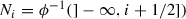. The filtration

  $$\begin{aligned} \varnothing = N_{-1}\subset N_0\subset \cdots \subset N_r =N \end{aligned}$$

  where $r=\dim N$ is called the Morse–Smale filtration associated to $\phi$ (or MS-filtration for brevity).

• For a given MS-filtration $\{N_i\}$ of N, the filtration by submanifolds is also an MS-filtration, called the dual MS-filtration of the filtration $\{N_i\}$.

Remark 9.2

The term $N_s$ of an MS-filtration is the result of attaching to $N_{-1}$ of handles of indices $\leqslant s$; it is a manifold with boundary homotopy equivalent to an s-dimensional CW complex.

Definition 9.3

An f-gradient v is called almost transverse if $D(p,v) \pitchfork D(q, -v)$ whenever $\mathrm{ind}\,p \leqslant \mathrm{ind}\,q$. The set of all f-gradients is denoted by G(f), the set of all almost transverse f-gradients is denoted by $G_{\mathrm{A}}(f)$, the set of all transverse f-gradients is denoted by $G_{\mathrm{T}}(f)$.

Definition 9.4

Let $f:W\rightarrow [a,b]$ be a Morse function on a cobordism W, v an f-gradient, and v an almost transverse f-gradient. We say that v satisfies the condition $({\mathfrak {C}})$ if there is a Morse–Smale filtration $\{\partial _1 W^k\}$ of $\partial _1 W$ and a Morse–Smale filtration $\{\partial _0 W^k\}$ of $\partial _0 W$ such that for every k,

The gradients satisfying the condition $({\mathfrak {C}})$ will be also called cellular gradients, or ${\mathfrak {C}}$-gradients. The set of all cellular gradients of f will be denoted by $G_{\mathrm{C}}(f)$.

The following theorem is one of the main results of [15], we cite it here using the terminology of [13, Part 3].

Theorem 9.5

The subset $G_{\mathrm{C}}(f)\subset G_{\mathrm{A}}(f)$ is open and dense in $C^0$-topology.

Let v be a cellular f-gradient for a Morse function f on a cobordism W. Consider the compact topological space $\partial _1 W{}^k/\partial _1 W{}^{k-1}$ obtained by shrinking the subspace $\partial _1 W^{k-1}$ to a point denoted $r_{k-1}$. The image of a point $y\in \partial _1 W^k$ in the space $\partial _1 W^k/\partial _1 W^{k-1}$ will be denoted by ${\overline{y}}$. Similar notation will be used for $\partial _0 W$, the shrunk subspace $\partial _0 W^{k-1}$ will be denoted by $s_{k-1}$. The next theorem describes the cellular-like structure on the map ${(-v)}^{\rightsquigarrow }$ (see [13, p. 234]).

Theorem 9.6

If v is a cellular f-gradient then for every k there is a continuous map

$$\begin{aligned} {(-v)}^{\displaystyle \twoheadrightarrow }:\partial _1 W^k/\partial _1 W^{k-1} \rightarrow \partial _0 W^k/\partial _0 W^{k-1} \end{aligned}$$

such that ${(-v)}^{\displaystyle \twoheadrightarrow }(r_{k-1}) = s_{k-1}$ and

$$\begin{aligned}&{(-v)}^{\displaystyle \twoheadrightarrow }(\overline{x}) = s_{k-1}&\quad \text {if}\;\; x\in D(-v), \\&{(-v)}^{\displaystyle \twoheadrightarrow } (\overline{x}) =\overline{{(-v)}^{\rightsquigarrow }(x)}&\quad \text {if}\;\; x\notin D(-v). \end{aligned}$$

Definition 9.7

The map induced by ${(-v)}^{\displaystyle \twoheadrightarrow }$ in homology is denoted by

and called the homological gradient descent.

This homomorphism is stable with respect to $C^0$-small perturbations of the gradient, as shown in [13, p. 282]:

Proposition 9.8

Let v be a cellular gradient of a Morse function $f:W\rightarrow [a,b]$. There is $\delta >0$ such that for every f-gradient w with $\Vert w-v\Vert <\delta$ the homomorphisms

are equal.

1.1.2 Cellular gradients for circle-valued Morse functions and their Novikov complexes

Let $f:M\rightarrow S^1={{\mathbb {R}}}/{{\mathbb {Z}}}$ be a Morse function, we will assume that its class [f] in $H^1(M,{{\mathbb {Z}}})$ is indivisible. Let $\overline{M} \rightarrow M$ be the corresponding infinite cyclic covering; lift the function f to a real-valued Morse function $F:\overline{M}\rightarrow {{\mathbb {R}}}$. Let $\lambda$ be a regular value of F, put $V=F^{-1}(\lambda )$. We have a cobordism $W=F^{-1}([\lambda -1,\lambda ])$ and a Morse function . Let t be a generator of the structure group $\approx {{\mathbb {Z}}}$ of the covering, such that . The map $t^{-1}$ determines a diffeomorphism $\partial _0 W\rightarrow \partial _1 W$ which will be denoted by I. An f-gradient v induces an F-gradient, denoted by the same symbol v.

Definition 9.9

• An f-gradient v is called cellular with respect to $\lambda$ if the induced F-gradient on W is cellular with respect to some MS-filtration $\{N_i\}$ on $\partial _0 W$ and the MS-filtration $\{I(N_i)\}$ on $\partial _1 W$.

• An f-gradient v is called cellular if it is cellular with respect to $\lambda$ for some regular value $\lambda$ of f.

• The set of all cellular gradients of f is denoted $G_{\mathrm{C}}(f)$.

The following theorem is one of the main results of [15], concerning circle-valued Morse functions; we cite it here in the terminology of [13, Chapter 12].

Theorem 9.10

• (i) The subset $G_{\mathrm{C}}(f)\subset G(f)$ is open and dense in G(f) with respect to $C^0$-topology.

• (ii) The subset $G_{\mathrm{C}}(f)\cap G_{\mathrm{T}}(f)\subset G_{\mathrm{T}}(f)$ is open and dense in $G_{\mathrm{T}}(f)$ with respect to $C^0$-topology.

Let v be a cellular f-gradient. For every k we have an endomorphism

Proposition 9.8 implies the following corollary.

Corollary 9.11

Let v be a cellular f-gradient. There is $\delta >0$ such that for every f-gradient w with $\Vert v-w\Vert <\epsilon$ and every r we have .

It turns out that the Novikov complex $N_*(f,v)$ can be computed in terms of this homomorphism. Let . Choose the lifts ${\bar{p}}, {\bar{q}}$ of the points p, q to $\overline{M}$ in such a way that ${\bar{p}}, {\bar{q}} \in t^{-1}W$. Since v is cellular, the k-dimensional submanifold $T=D({\bar{p}},v)\cap \partial _1 W$ is in $\partial _1 W^k$, and the set is compact. Choose some orientations of descending discs D(p, v), D(q, v). We have then the fundamental class . Assume for simplicity of exposition that M is oriented. Similarly, the $(r-k)$-dimensional submanifold $S=D( t{\bar{q}}, -v)\cap \partial _1 W$ determines a class

$$\begin{aligned}{}[S]\in H_{r-k}\bigl (\widehat{\partial }_1 W{}^{r-k}, \widehat{\partial }_1 W{}^{r-k-1}\bigr ), \end{aligned}$$

where $r=\dim V=\dim M -1$. The intersection index $\langle [T], [S] \rangle \in {{\mathbb {Z}}}$ is defined. The next theorem (see [13, p. 379]) expresses the Novikov incidence coefficient in terms of the gradient descent homomorphism.

Theorem 9.12

We have

(Here $n_0(p,q;v)\in {{\mathbb {Z}}}$ is the incidence coefficient of the critical points p, q in the cobordism W; the brackets denote the intersection index.)

The next corollary is obtained by a standard argument from linear algebra.

Corollary 9.13

For any cellular gradient v the Novikov incidence coefficient N(p, q; v) is a rational function of the form where and $Q(0)=1$.

1.2 An example

Let ${{\mathbb {T}}}^2$ be the 2-dimensional torus, $\alpha$ be its parallel, $\beta$ its meridian. Consider two disjoint closed discs $D_1, D_2$ in ${{\mathbb {T}}}^2$ which do no intersect $\alpha \cup \beta$. Removing their interiors from ${{\mathbb {T}}}^2$ we obtain a surface S, whose boundary is the disjoint union of two circles $\partial _1 S$ and $\partial _2 S$ (see the upper image on Fig. 1). Attach a copy S(1, 1) of S to another copy S(1, 2) of S, identifying $\partial _2 S(1,1)$ with $\partial _1 S(1,2)$. We obtain a surface of genus 2 with two components of boundary: $\partial _1 S(1,1)$ and $\partial _2 S(1,2)$. Attaching the copies $D_1(1), D_2(1)$ of the discs $D_1, D_2$ to these components gives a closed surface N of genus 2. One more copy of this surface will be denoted by K (see the bottom of Fig. 1).

Fig. 1

Construction of the manifold N

Similarly we glue together three copies S(1 / 2, 1), S(1 / 2, 0), S(1 / 2, 2) of S and attach to it two discs $D_1(1/2), D_2(1/2)$ to obtain a closed surface L of genus 3 (depicted in the middle of the figure). Associate to every point in $D_1(1/2)\cup S(1/2,1) \cup S(1/2,0)$ its copy in $D_1(1)\cup S(1,1)\cup S(1,2)$; this determines a diffeomorphism which will be denoted by I(1 / 2, 1). Similarly, we construct a diffeomorphism I(1 / 2, 0) of the surface $S(1/2,0)\cup S(1/2,2)\cup D_1(1/2)$ onto $S(0,1)\cup S(0,2) \cup D_2(0)$. A surgery along the circle $\beta (1/2, 2)$ yields a surface naturally diffeomorphic to N. Attaching the corresponding handle of index 2 to gives a cobordism $W_1$ endowed with a Morse function $F_1:W_1\rightarrow [1/2, 1]$. This Morse function has one critical point $x_2$ of index 2. Pick a gradient $w_1$ for this function in such a way that:

• (A1) The ascending disc $D(x_2, -w_1)$ intersects the level surface $N=F^{-1}_1(1)$ by two points in the interior of $D_2(1)$.

• (A2) The diffeomorphism $\overset{\rightsquigarrow }{w_1}$ sends $D_2(1/2)$ to the interior of $D_2(1)$.

• (A3) The restriction of $\overset{\rightsquigarrow }{w_1}$ to $D_1(1/2)\cup S(1/2,1)\cup S(1/2,0)$ equals I(1 / 2, 1) everywhere except a small tubular neighbourhood $T_1$ of the circle $\partial D_1(1/2)$. Further, $\overset{\rightsquigarrow }{w_1} (T_1) = I(1/2, 1) (T_1)$ and the $\overset{\rightsquigarrow }{w_1}$-image of $D_1(1/2)$ contains $D_1(1)$ in its interior.

Similarly, we do a surgery along the circle $\beta (1/2,1)$ and obtain a surface naturally diffeomorphic to K. Attach the corresponding handle to , get a cobordism $W_0$ endowed with a Morse function $F_0:W_0\rightarrow [0,1/2]$ having one critical point $x_1$ of index 1. Pick an $F_0$-gradient $w_0$ such that:

• (B1) The descending disc $D(x_1, w_0)$ intersects the level surface $K=F^{-1}_0(0)$ by two points in the interior of $D_1(0)$.

• (B2) The diffeomorphism ${(-w_0)}^{\rightsquigarrow }$ sends $D_1(1/2)$ to the interior of $D_1(0)$.

• (B3) The restriction of ${(-w_0)}^{\rightsquigarrow }$ to $S(1/2,0)\cup S(1/2,2)\cup D_1(1/2)$ equals I(1 / 2, 0) everywhere except a small tubular neighbourhood $T_2$ of the circle $\partial D_2(1/2)$. Further, ${(-w_0)}^{\rightsquigarrow }(T_2) = I(1/2, 0) (T_2)$ and the ${(-w_0)}^{\rightsquigarrow }$-image of $D_2(1/2)$ contains $D_2(0)$ in its interior.

We have $\partial W_1 \approx N\sqcup L$, $\partial W_0 \approx L\sqcup K$; attaching $W_1$ to $W_0$ along the L-component of their boundaries we obtain a cobordism W with boundary $\partial W\approx N\sqcup K$, endowed with a Morse function $F:W\rightarrow [0,1]$, such that , . The gradients $w_0$ and $w_1$ can be glued together (modifying them appropriately nearby L if necessary) so that the resulting gradient w is cellular F-gradient (see Definition 9.4). To show this we introduce Morse–Smale filtrations on $\partial _0 W$ and $\partial _1 W$. Let

$$\begin{aligned} N_0=D_1(1), \quad N_1 = D_1(1) \cup S(1,1)\cup S(1,2), \quad N_2= N. \end{aligned}$$

The filtration $N_0\subset N_1\subset N_2$ is then an MS-filtration of N. The image of this filtration with respect to the natural diffeomorphism $J:N \rightarrow K$ is an MS-filtration $K_0\subset K_1 \subset K_2$ on K. Properties (A1)–(A3) and (B1)–(B3) imply the following:

$$\begin{aligned}&\mathrm{(D1)}&\qquad D(x_i, w) \cap \partial _0 W\subset \mathrm{Int}\,K_{i-1} \quad \text {for}\;\; i=1,2, \\&\mathrm{(D2)}&\qquad {(-w)}^{\rightsquigarrow } (N_i) \subset \mathrm{Int}\,K_i \quad \text {for}\;\; i=0,1,2. \end{aligned}$$

We have also the dual properties

$$\begin{aligned}&\mathrm{(U1)}&\qquad D(x_i, -w) \cap \partial _1 W\subset \mathrm{Int}\,{\widehat{N}}_{2-i} \quad \text {for} \;\; i=1,2, \\&\mathrm{(U2)}&\qquad \overset{\rightsquigarrow }{w} ({\widehat{K}}_i) \subset \mathrm{Int}\,{\widehat{N}}_i \quad \text {for} \; \;i=0,1,2 \end{aligned}$$

(recall that ${\widehat{N}}_i$ and ${\widehat{K}}_i$ denote the MS-filtrations dual to the filtrations $N_i$, resp. $K_i$). The conjunction of properties (D1), (D2) is just a reformulation of the condition ($\mathfrak {C}$1); similarly the conjunction of properties (U1), (U2) is equivalent to ($\mathfrak {C}$2). The F-gradient w is therefore cellular.

The 3-manifold M and a circle-valued function on it will be obtained by gluing N to K via a diffeomorphism that we will now describe. Put

$$\begin{aligned} a_1=[\alpha (1,1)], \quad a_2=[\alpha (1,2)], \quad b_1=[\beta (1,1)], \quad b_2=[\beta (1,2)]. \end{aligned}$$

The family is then a basis in $H_1(N)$. The same embedded circles determine the homology classes in $H_1(N_1/N_0)$, they will be denoted by the same letters by a certain abuse of notation. Similarly we obtain a base in $H_1(K)$ and $H_1(K_1/K_0)$. Denote by $J:N\xrightarrow { \, \approx \,} K$ the natural diffeomorphism, then we have . Consider the automorphism of $H_1(K)\approx {{\mathbb {Z}}}^4$ given in the base by the following matrix:

$$\begin{aligned} {{\mathfrak {S}}}=\left( \begin{matrix} 0 &{} \quad 2 &{} \quad 1 &{}\quad 0\\ 0 &{}\quad 0 &{}\quad 0 &{} \quad 1\\ 0 &{}\quad 1 &{}\quad 0 &{}\quad 0\\ -1 &{}\quad q &{} \quad 0 &{} \quad -2\\ \end{matrix} \right) \end{aligned}$$

where q is any integer $\geqslant 3$. It is easy to check that ${{\mathfrak {S}}}$ preserves the intersection form on $H_1(N)$ therefore there is a diffeomorphism $\Phi :K\rightarrow K$ inducing ${{\mathfrak {S}}}$ in $H_1$. We can assume that $\Phi (x)=x$ for $x\in D_1(0)\cup D_2(0)$. Identifying each point $y\in K$ with $J\Phi (y)\in N$ we obtain a 3-manifold M; the Morse function F induces a map $f:M\rightarrow S^1$. The F-gradient w induces an f-gradient v. Observe that v is a cellular f-gradient with respect to regular level surface N and its MS-filtration $\{N_i\}$. The matrix of the endomorphism is easy to compute; it equals

$$\begin{aligned} {{\mathfrak {M}}}= \left( \begin{matrix} 0 &{}\quad 0 &{}\quad 0 &{}\quad 2\\ 0 &{}\quad 0 &{}\quad 0 &{}\quad 0\\ 0 &{}\quad 0 &{}\quad 0 &{} \quad 1\\ 0 &{}\quad 0 &{}\quad -1 &{}\quad q \end{matrix} \right) . \end{aligned}$$

Pick a transverse f-gradient u sufficiently close to v in $C^{\infty }$ topology so that u is still a cellular f-gradient with respect to the level surface N and its MS-filtration $\{N_i\}$, and . The Novikov incidence coefficient $N( x_2, x_1; u)$ is now easy to compute. Let T be the $J^{-1}$-image in N of $D(x_2,u)\cap K$, and $\theta =[T]\in H_1(N_1/N_0)$. Then $\theta =b_1-2b_2$. Let $S=D(x_1,-u)\cap N$ then $[S]=b_1\in H_1(N_1/N_0)$. Applying Theorem 9.12 we obtain

$$\begin{aligned} n_{k+1}( x_2, x_1; u) = \big \langle {{\mathfrak {M}}}^k(\theta ), b_1\big \rangle . \end{aligned}$$

We have . Therefore $n_{k+1}( x_2, x_1; u)$ equals the first coordinate of the vector with respect to basis . Computing this first coordinate is a routine exercise in linear algebra which will be left to the reader. We give just the result:

(17)

The properties of f and v stated in the beginning of this appendix are now obvious.

References

Boyd, S., Vandenberghe, L.: Convex Optimization. Cambridge University Press, Cambridge (2004)
Bruns, W., Gubeladze, J.: Polytopes, Rings, and \(K\)-Theory. Springer Monographs in Mathematics. Springer, Dordrecht (2009)
Cohn, P.M.: Skew Fields. Encyclopedia of Mathematics and Its Applications, vol. 57. Cambridge University Press, Cambridge (2011)
Farber, MSh: Sharpness of the Novikov inequalities. Funct. Anal. Appl. 19(1), 40–48 (1985)
Farrell, F.T., Hsiang, W.-C.: A formula for \(K_{1}R_{\alpha }\,[T]\). In: Heller, A. (ed.) Applications of Categorical Algebra, pp. 192–218. American Mathematical Society, Providence (1970)
Floer, A.: Symplectic fixed points and holomorphic spheres. Comm. Math. Phys. 120(4), 575–611 (1989)
Goldie, A., Michler, G.: Ore extensions and polycyclic group rings. J. London Math. Soc. (2)9, 337–345 (1974/1975)
Latour, F.: Existence de \(1\)-formes fermées non singulières dans une classe de cohomologie de de Rham. Inst. Hautes Études Sci. Publ. Math. 80, 135–194 (1995)
Laudenbach, F., Moraga Ferrándiz, C.: A geometric Morse–Novikov complex with infinite series coefficients. C. R. Math. Acad. Sci. Paris 356(11–12), 1222–1227 (2018)
Novikov, S.P.: Multivalued functions and functionals. An analogue of the Morse theory. Dokl. Akad. Nauk SSSR 260(1), 31–35 (1981) (in Russian)
Ore, O.: Theory of non-commutative polynomials. Ann. Math. 34(3), 480–508 (1933)
Pajitnov, A.: Incidence coefficients in the Novikov complex for Morse forms: rationality and exponential growth properties (1996). arxiv:dg-ga/9604004
Pajitnov, A.V.: Circle-Valued Morse. Theory De Gruyter Studies in Mathematics, vol. 32. de Gruyter, Berlin (2006)
Pazhitnov, A.V.: On the Novikov complex for rational Morse forms. Ann. Fac. Sci. Toulouse Math. 4(2), 297–338 (1995)
Pazhitnov, A.V.: Rationality of boundary operators in the Novikov complex in general position. St. Petersburg Math. J. 9(5), 969–1006 (1998)
Pitcher, E.: Critical points of a map to a circle. Proc. Natl. Acad. Sci. USA 25(2), 428–431 (1939)
Poźniak, M.: Floer homology, Novikov rings and clean intersections. In: Eliashberg, Ya., et al. (eds.) Northern California Symplectic Geometry Seminar. American Mathematical Society Translations, Series 2, vol. 196, pp. 119–181. American Mathematical Society, Providence (1999)
Salamon, D.: Morse theory, the Conley index and Floer homology. Bull. London Math. Soc. 22(2), 113–140 (1990)
Schütz, D.: On the Whitehead group of Novikov rings associated to irrational homomorphisms. J. Pure Appl. Algebra 208(2), 449–466 (2007)
Sikorav, J.C.: Points fixes de difféomorphismes symplectiques, intersections de sous-variétés lagrangiennes, et singularités de un-formes fermées. Ph.D. thesis, Université Paris-Sud (1987)
Witten, E.: Supersymmetry and Morse theory. J. Differential Geom. 17(4), 661–692 (1982)
Acknowledgements
I am indebted to Andrew Ranicki for many discussions on circle-valued Morse theory. I am grateful to Günter Ziegler for the references about integral cones and to Joseph Gubeladze for nice and helpful discussion about bases in integral cones. Thanks to the anonymous referee, whose remarks have lead to a considerable improvement of the manuscript. Many thanks to Fedor Bogomolov for his constant support.
Author information
Authors and Affiliations
Corresponding author
Additional information
Dedicated to the memory of Andrew Ranicki
Publisher's Note
Springer Nature remains neutral with regard to jurisdictional claims in published maps and institutional affiliations.