
Abstract
This paper presents a novel integrated framework for simulating the charging load of an electric vehicle charging station. The framework is built based on the cellular automaton model, including five modules: vehicle generation, charging station, lane change, speed update and boundary clear. The proposed framework can effectively stimulate the system dynamics of the traffic system and charging power process in a charging station. Case studies have verified its feasibility and effectiveness.
1 Introduction
Transportation electrification has been regarded as one of the most promising solutions for petroleum consumption reduction and environmental protection. In recent years, the government regards promoting the development of electric vehicles (EVs) and construction of charging facilities as national strategic initiatives. The construction of charging facilities needs to be adapted to the configuration of electricity and transportation [1]. It is necessary to pre-evaluate the potential charging demand of a charging station (CS) before planning and the simulation of the charging load of the CS is the basis for this work. Similar to power load forecasting approximation, the scenario, neural network and other methods [2, 3] have been introduced to study charging load. However, the charging load depends on the behavior of the EV itself, in which the charging events primarily occur in the CS, where the movement and space-time characteristics need to be fully considered in order to achieve an accurate calculation. Thus the charging load approximation or forecasting would be different from those for electricity.
In addition, conventional methods usually rely on a large amount of data. But at present, EVs are still in the early stage of development. Due to the lack of actual data, only the travel statistics of traditional fuel vehicles, along with information from a small number of EVs and some traffic flow information are available to model probabilistic EV charging. Additionally, the queuing theory, stochastic probability method, etc. [1, 4,5,6,7,8], are used to simulate EV driving and charging characteristics. For example, a traffic flow integrated model was used to stimulate the mobile charging load for CS planning in [1]. The large scale adoption of EVs will have a great influence on transportation and power industries. In addition, the traditional methods, which can be used to calculate the charging load, were primarily from a macro perspective, but it is not convincing when performing CS planning for a specific road, as an example. In this case, the charging demand is highly related to road conditions, traffic flow, different behaviors of different types of vehicles and the remaining power available in different time periods. The number and behaviors of EVs are not experimentally known so far due to the relative scarcity of EVs on the road. It is hard to simulate the charging demand un-constructed by using conventional methods when the real data is absent, which is supposed to be used to provide guidance for charging load assessment of the candidate CS deployments.
In this paper, a discrete cellular automaton (CA) model is introduced to simulate the behaviors of EVs and the related traffic-power conditions from the microcosmic view, which is supposed to capture the interactive impacts of factors in coupled systems, such as vehicle speed, charging expectation (CE), road conditions, state of charge (SOC), etc. Although CA has also been studied in the field of traffic simulation with several achievements [9, 10], jointly simulating EV behavior and charging load of the CS with traffic flow is rare. Therefore, this paper provides a way to investigate the charging load simulation from a CS perspective and proposes a simple but novel integrated “traffic-power” simulation framework.
2 Simulation framework with CA
A CA is a computer-based simulation technology where each cell may exist in a number of different discrete states. The transition from one state to another is governed by its specific rule sets, which can either be completely deterministic or stochastic in nature [9]. The key motivation of adopting CA technology to the problem at hand is to make the discrete cellular entities analogous to the allocation or behavior within the real world. In this study, the cell corresponds to a single vehicle, as indicated by the red points shown in Fig. 1.

CA space for simulation
The behavior of a vehicle is governed by a set of rules, reflected by the attribute matrixes, primarily including vehicle speed, vehicle type, charging expectation, charging timing, remaining battery capacity, charging power and total charging load, which are updated according to the rules designed in the simulation framework. It primarily includes five modules, as shown in Fig. 2.

Traffic-power simulation framework
3 Modules for simulation
The traffic-power simulation framework consists of five modules, as presented below.
3.1 Vehicle generation module
In this module, the generation of new vehicles is triggered when the first road cell is empty and its average arrival condition is reflected by the traffic flow data. Then the main four attributes of the new vehicle could be obtained, including type, speed, remaining SOC and CE. Each of them is modeled as follows. The type of the new vehicle (traditional vehicle or EV) is stochastically generated according to the given EV penetration level, defined as EVP. The vehicle speed is categorized into five levels, quantified from 1 to 5. Considering that very few vehicles run at a low speed, the initial speed is set from 2 to 5, which follows a uniform distribution at the same time. The average arrival number of vehicles in each time period can be reflected by the traffic flow data. The initial remaining SOC of each EV can be generated by specific distribution functions formulated according to historical statistics [11]. Due to fact that the charging expectation of a vehicle is affected by various factors, for simplicity, the most influential factor, i.e., the remaining SOC, is used to formulate the CE-SOC equation in the letter.
3.2 CS module
In this module, the vehicle speed is set at level 1 at the road portion of the CS if it is going to be charged in order to reflect the real condition. Fast and slow charging are options according to its current SOC. For example, for an EV with a 30 kWh capacity battery, 6 hours (total charging time) are needed if slow charging with 5 kW is utilized, while it would require 1 hour with fast charging at 30 kW. Thus, the formula for the remaining charging time \(T_{\text{c}}\) is:
where \(SOC_{{{\rm p}.{\rm u}.}}\) is the nominal remaining SOC of the EV; T is the total time of fast or slow charging. Let FS be the criteria for choosing the fast charging if \(SOC_{{{\rm p}.{\rm u}.}} \le FS\), otherwise the slow charging will be utilized. It is also noted that charging in the CS follows the “first out, first in” rule, which is determined by the availability of the charging devices. Then the charging load of the CS can be accumulated according to the charging conditions (charging type and its unit charging power) of the charging devices.
3.3 Lane change module
The lane change module is implemented to realize the location and state transfer of the EV when there is congestion in front or entering the junction as shown in Fig. 1, where the attribute matrixes are adopted as transfer criteria. In terms of the traditional vehicles or EVs which do not need to be charged, the Nagel-Schreckenberg (NS) lane change rule [9] would be directly implemented. Regarding the EVs to be charged, the lane change at the junction to the CS road needs to be considered in the state updates of the corresponding attribute matrix.
3.4 Speed update module
In addition to implementing the basic NS speed update rules [9], other specific rules will be added and utilized in this module. For the vehicles may not really speed up even if the NS speed up rules are met, the speed up probability is introduced to indicate this scenario. The speed down probability is assumed to be 1 in the case of traffic danger.
3.5 Boundary clear module
All attributes in the “Boundary” space, as shown in Fig. 1, will be cleared in each time period to maintain the equilibrium of the dynamic system. With the provided temporal traffic flow profiles and other inputs, the attribute matrixes can be automatically updated and the dynamic charging load of the specific CS could be simulated, based on the proposed traffic-power simulation framework which includes all above modules, i.e., evolution rules for the CA model.
4 Case study
The one road designed in Fig. 1 is adopted as the test system. 30 charging devices are installed in the CS. It is assumed that the average battery of an EV is 30 kWh and the charging power of fast charging is set as 30 kW while the slow charging is 5 kW. Let EVP = 5%, FS = 0.7. The quantity of the CE is determined by several factors, and for simplicity, only the initial remaining SOC is employed to obtain the quantity of CE by using a proximate equation [12]: \(CE = 0.1^{SOC_{{\rm p}.{\rm u}.}}\). Figure 3 shows the typical daily traffic flow profile per a half hour according to [13]. The initial remaining SOC is generated based on the given piecewise uniform distribution function, formulated over a day, and used in the cases for example:
Selecting a day as the simulation period cycle, the results based on the proposed framework are shown in Fig. 4. The evolution of the charging load in the day is consistent with that of the traffic flow profile in Fig. 3. For example, at around 07:00, there is a power peak due to the accumulated EVs’ charging in the CS, which is also a peak time for people to leave home for work. Although CE is not large in that time period, heavier traffic also contributes to large charging load demand, as shown in Fig. 4. A similar case appears during off-work time periods. However, the charging load curve is relatively flat during some heavy traffic periods because a number of EVs may have been charged at the charging piles of the workplace rather than at the CS. Thus, the SOC can remain at a high level when it arrives at the road portion. That is the reason why the charging power of the CS during the off-work time seems to be less than that in the morning of the day, even though the traffic is heavier.

Typical daily traffic flow

Daily charging load simulation results
To investigate the impacts of input parameter variations, two extended cases are simulated.
-
1)
In the CS module, FS is used to indicate whether fast or slow charging is chosen. Simulate the charging load of the CS in eight scenarios (days) with different FS settings (0.1~0.8), respectively. The results are shown in Fig. 5. Generally, the charging load profile shows a climbing trend, while the details in different scenarios vary dramatically. For example, the curves are similar when FS ∊ {0.1, 0.2, 0.3} and the peak load is less than 200 kW. The curve starts to be sharp when FS is larger than 0.4 and the curve becomes much sharper and contributes over 600 kW when FS = 0.8. FS determines the choice of fast or slow charging, according to the SOC of the new generated EV. Larger FS indicates that with a larger possibility, fast charging would be chosen. In this case, with the current inputs and CS deployment, 0.4 would be the segmentation point of FS setting for charging load simulation in different similar profiles.
Fig. 5 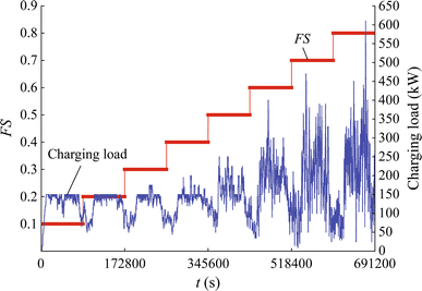
Charging load simulation results with different FS settings
-
2)
The setting of EVP may also affect the charging load simulation. Simulate the charging load of the CS in eight scenarios (days) with different EVP settings (5%~40%), respectively. The results are shown in Fig. 6. EVP indicates the average penetration level of the EVs in the total vehicles, which draws an analogy on the traffic flow to generate and illustrate whether the new vehicle is EV or not. As illustrated in Fig. 6, the charging load generally grows with the increasing EVP from 5%~10%. In addition, the charging load profile seems similar when EVP varies from 15% to 40% because of the limitation of the CS deployment with 30 charging devices and the input conditions. Thus, from the case study, it can be summarized that the increasing penetration level of the EVs could possibly increase the charging load level of the CS, but the final quantity is affected by its scale, i.e., the deployment of the charging devices. In this case, demand for CS expansion is desirable with the increasing penetration level of the EVs.
Fig. 6 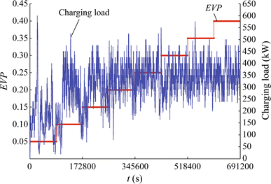
Charging load simulation results with different EVP settings


5 Conclusion
In this paper, an integrated traffic-power simulation framework based on CA is designed. It captures the dynamic behaviors of the interactions between the evolution coherence of charging loads and traffic flows, as presented in the test cases. This study is very beneficial for charging load quantification and can also be employed for evaluating the feasibility of EV CS deployments.
References
Xiang Y, Liu JY, Ran Li et al (2016) Economic planning of electric vehicle charging stations considering traffic constraints and load templates. Appl Energy 178:647–659
Mukherjee JC, Gupta A (2017) Distributed charge scheduling of plug-in electric vehicles using inter-aggregator collaboration. IEEE Trans Smart Grid 8(1):331–341
Panahi D, Deilami S, Masoum MAS et al (2015) Forecasting plug-in electric vehicles load profile using artificial neural networks. In: Proceedings of 2015 Australasian universities power engineering conference (AUPEC), Wollongong, Australia, 27–30 September 2015, 6 pp
Shuai W, Maillé P, Pelov A (2016) Charging electric vehicles in the smart city: a survey of economy-driven approaches. IEEE Trans Intell Transp Syst 17(8):2089–2106
Tian L, Shi S, Jia Z (2010) A statistical model for charging power demand of electric vehicles. Power Syst Technol 34(11):126–130
Omran NG, Filizadeh S (2014) Location-based forecasting of vehicular charging load on the distribution system. IEEE Trans Smart Grid 5(2):632–641
Zhang HC, Hu ZC, Xu ZW et al (2017) Optimal planning of PEV charging station with single output multiple cables charging spots. IEEE Trans Smart Grid 8(5):2119–2128
Wang ZP, Liu P (2010) Analysis on storage power of electric vehicle charging station. In: Proceedings of IEEE Asia-Pacific power and energy engineering conference, Chengdu, China, 28–31 March 2010, 5 pp
Jia B, Gao Z, Li K et al (2007) Models and simulations of traffic system based on the theory of cellular automation. Science Press of China, Beijing
Zheng Y, Zhai R, Ma S (2006) Survey of cellular Automata model of traffic flow. J Highway Transp Res Dev 23(1):110–115
Xiang Y, Liu JY, Liu Y (2016) Optimal active distribution system management considering aggregated plug-in electric vehicles. Electric Power Syst Res 131:105–115
Tao S, Xiao XN, Wen JF et al (2014) Configuration ratio for distributed electrical vehicle charging infrastructures. Trans China Electr Soc 29(8):11–19
Xiang Y, Liu JY, Tang SY et al (2015) A traffic flow based planning strategy for optimal siting and sizing of charging stations. In: Proceedings of Asia-Pacific power energy engineering conference, Brisbane, Australia, 15–18 November 2015, 5 pp
Acknowledgements
This work was supported by National Natural Science Foundation of China (No. 51377111), Fundamental Research Funds for the Central Universities (No. YJ201654) and Open Research Subject of Key Laboratory of Sichuan Power Electronics Energy-saving Technology and Devices (No. szjj2017-052).
Author information
Authors and Affiliations
Corresponding author
Additional information
CrossCheck date: 27 December 2017
Rights and permissions
Open Access This article is distributed under the terms of the Creative Commons Attribution 4.0 International License (http://creativecommons.org/licenses/by/4.0/), which permits unrestricted use, distribution, and reproduction in any medium, provided you give appropriate credit to the original author(s) and the source, provide a link to the Creative Commons license, and indicate if changes were made.
About this article

Cite this article
XIANG, Y., LIU, Z., LIU, J. et al. Integrated traffic-power simulation framework for electric vehicle charging stations based on cellular automaton. J. Mod. Power Syst. Clean Energy 6, 816–820 (2018). https://doi.org/10.1007/s40565-018-0379-3
Received:
Accepted:
Published:
Issue Date:
DOI: https://doi.org/10.1007/s40565-018-0379-3