
Abstract
This paper presents new results on the welfare effects of third-degree price discrimination under constant elasticity demand. We show that when both the share of the strong market under uniform pricing and the elasticity difference between markets are high enough, then price discrimination not only can increase social welfare but also consumer surplus. We also obtain new bounds on the welfare change for log-convex demands.


Notes
There is some previous research on this aspect. Greenhut and Ohta (1976) show numerically that price discrimination may increase output, and Ippolito (1980) finds that total output increases in all his numerical simulations. Formby et al. (1983) use Lagrangean techniques to show that discrimination increases total output over a wide range of constant elasticities. Finally, Aguirre (2006) provides an analytical proof using an inequality due to Bernoulli and ACV simplify and slightly generalize the proof (which uses the fact that demand is convex in the reciprocal of the price).
Ippolito (1980) shows using numerical simulations that price discrimination can increase social welfare and consumer surplus.
Nahata et al. (1990) show that the profit function is concave for prices below \(\bar{p}=(\varepsilon _i +1)c/(\varepsilon _i -1)\) and convex for higher prices.
The aggregate profit function would be concave (and therefore quasi-concave) in the relevant range of prices if \(\pi ^{''}( p) <0 \forall p\in [p_2^*,p_1^*]\). Note that \(\pi ^{''}( p) < 0 \forall p\in [p_2^*,\bar{p}_2 ]\) given the shape of the profit function in market 2. Therefore, a sufficient condition for concavity of the profit function is \(p_1^*\le \bar{p}_2 \) or, alternatively, \(\varepsilon _2 \le 2\varepsilon _1 -1\).
All markets are automatically served under uniform pricing.
For example, when \(\varepsilon _1 =4\) if the elasticity difference is \(\theta =17\) then for \(\alpha \in ({0,0.797})\mathop \cup \nolimits (0.9,0.999)\) the global maximizer is \(p=1\). When \(\alpha \in ({0.797, 0.9})\) the optimal uniform price can be higher or lower than \(p=1\). As Table 1 indicates, when \(\varepsilon _1 =4\) and \(\theta \in (0,16.9)\) the aggregate profit function reaches a global maximum at \(p=1\).
We consider the case of quasi-linear utility function with an aggregate utility function of the form \(\mathop \sum \nolimits u_i ( {q_i })+y_i \), where \(q_i \) is consumption in market \(i \)and \(y_i \) is the amount to be spent on other goods. The sub-utilities \(u_i \), \(i=1,2\), are increasing and strictly concave.
See Quah and Strulovici (2012).
Numerical computations allow us to conclude that \({\theta }^{\prime }(\varepsilon _1 )>0\).
Fig. 1 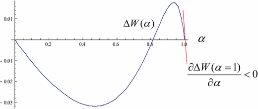
Single-crossing property. The change in welfare as a function of \(\alpha \)
Of course, \(\tilde{\theta }(\varepsilon _1 )>{\underline{\theta }}(\varepsilon _1)\). For instance, \(\tilde{\theta }( 2)=7>1.3102={\underline{\theta }}(2)\) or \(\tilde{\theta }( 3)=11.9>1.3616={\underline{\theta }}(3)\).
See Weyl and Fabinger (2013) for an extensive analysis of pass-through.
Of course, \(\tilde{\theta }(\varepsilon _1 )>{{\underline{\underline{\theta }}}}(\varepsilon _1 )\). For instance, \(\tilde{\theta }( 2)=7>2.4091={{\underline{\underline{\theta }}}}(2)\) or \(\tilde{\theta }( 3)=11.9>5.1699={{\underline{\underline{\theta }}}}(3)\).
Lemma 3 might be equivalently enunciated in terms of inverse demand. That is, the cost pass-through coefficient exceeds 1 when \(p_i ( {q_i })-c\) is strictly log-convex. Amir (1996) uses the same property but to guarantee in a context of Cournot oligopoly that the game is log supermodular.
The strictly log-convex demand family is much wider than constant elasticity demand family. Mrázová and Neary (2013) classify strictly log-convex demands or demands with Super-Pass-Through taking as a base the family of constant elasticity demands (CES demands). They consider three types of strictly log-convex demands: strictly super convex demands, constant elasticity demands and strictly sub convex demands. Super convexity of a demand function at an arbitrary point is equivalent to the function being more convex at that point than a CES demand function with the same elasticity.
The lower bound for consumer surplus is the same as Varian’s lower bound for welfare.
Bulow and Klemperer (2012) illustrate how consumer surplus equals the area between the inverse demand curve and the marginal revenue curve up to a given quantity.
Note that the assumption \(\varepsilon _i >1, i=1,2\), guarantees that the profit function in market \(i \) (as a function of output) is strictly concave under constant elasticity demand.

References
Aguirre, I.: Monopolistic price discrimination and output effect under conditions of constant elasticity demand. Econom. Bull. 23(4), 1–6 (2006)
Aguirre, I., Cowan, S., Vickers, J.: Monopoly price discrimination and demand curvature. Am. Econ. Rev. 100, 1601–1615 (2010)
Aguirre, I., Cowan, S.: Monopoly price discrimination with constant elasticity demand. Ikerlanak Working Paper Series IL 74/13, University of the Basque Country UPV/EHU (2013)
Amir, R.: Cournot oligopoly and the theory of supermodular games. Games Econ. Behav. 15, 132–148 (1996)
Amir, R., Maret, I., Troege, M.: On taxation pass-through for a monopoly firm. Ann. D’Econ. Statisq. 75(76), 155–172 (2004)
Bulow, J., Klemperer, P.: Regulated prices, rent seeking, and consumer surplus. J. Polit. Econ. 120, 160–186 (2012)
Cheung, F., Wang, X.: Adjusted concavity and the output effect under monopolistic price discrimination. South. Econ. J. 60, 1048–1054 (1994)
Cowan, S.: The welfare effects of third-degree price discrimination with nonlinear demand functions. Rand J. Econ. 32, 419–428 (2007)
Cowan, S.: Third-degree price discrimination and consumer surplus. J. Ind. Econ 60, 333–345 (2012)
Formby, J.P., Layson, S., Smith, W.J.: Price discrimination, adjusted concavity, and output changes under conditions of constant elasticity. Econ. J. 93, 892–899 (1983)
Greenhut, M.L., Ohta, H.: Joan Robinson’s criterion for deciding whether market discrimination reduces output. Econ. J. 86, 96–97 (1976)
Ippolito, R.: Welfare effects of price discrimination when demand curves are constant elasticity. Atl. Econ. J. 8, 89–93 (1980)
Mrázová, M., Neary, J.P.: Not so demanding: preference structure, firm behavior, and welfare. Discussion Paper Series No. 691, University of Oxford (2013)
Nahata, B., Ostaszewski, K., Sahoo, P.K.: Direction of price changes in third-degree price discrimination. Am. Econ. Rev. 80, 1254–1262 (1990)
Pigou, A.C.: The economics of welfare, 3rd edn. Macmillan, London (1920)
Quah, John K.-H., Strulovici, Bruno: Aggregating the single crossing property. Econometrica 80, 2333–2348 (2012)
Robinson, J.: The economics of imperfect competition. Macmillan, London (1933)
Schmalensee, R.: Output and welfare implications of monopolistic third-degree price discrimination. Am. Econ. Rev. 71, 242–247 (1981)
Schwartz, M.: Third-degree price discrimination and output: generalizing a welfare result. Am. Econ. Rev. 80, 1259–1262 (1990)
Shih, J., Mai, C., Liu, J.: A general analysis of the output effect under third-degree price discrimination. Econ. J. 98, 149–158 (1988)
Varian, H.R.: Price discrimination and social welfare. Am. Econ. Rev. 75, 870–875 (1985)
Weyl, G., Fabinger, M.: Pass-through as an economic tool: principles of incidence under imperfect competition. J. Polit. Econ. 121, 528–583 (2013)
Acknowledgments
Financial support from the Ministerio de Economía y Competitividad (ECO2012-31626), and from the Departamento de Educación, Política Lingüística y Cultura del Gobierno Vasco (IT869-13) is gratefully acknowledged. We would like to thank Ilaski Barañano, Preston McAfee, Ignacio Palacios-Huerta and an anonymous referee for helpful comments.
Author information
Authors and Affiliations
Corresponding author
Appendix
Appendix
Proof of Lemma 1
where \(\Psi =\frac{\theta }{[\varepsilon _1 +( {1-\alpha })\theta -1]}\). It can be checked by numerical computations that \(\frac{\partial ^2\Delta W}{\partial \alpha ^2}\) crosses at most once the horizontal axis (we have checked numerically for \(\varepsilon _1 \in \{1.5,2,3,4,\ldots ,10\}\) and for any elasticity difference compatible with Assumption 1): this guarantees that the change in welfare is a convex–concave function of \(\alpha \).
Cross Derivative
where \(\Gamma =( {\frac{\varepsilon _1 (\varepsilon _1 +\theta -1)}{(\varepsilon _1 -1)(\varepsilon _1 +\theta )}})^{\varepsilon _1 +\theta -1}\). We have checked numerically that:
\(\square \)
Rights and permissions
About this article

Cite this article
Aguirre, I., Cowan, S.G. Monopoly price discrimination with constant elasticity demand. Econ Theory Bull 3, 329–340 (2015). https://doi.org/10.1007/s40505-014-0063-3
Received:
Accepted:
Published:
Issue Date:
DOI: https://doi.org/10.1007/s40505-014-0063-3