
Abstract
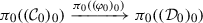
We study the homotopy theory of \(\infty \)-categories enriched in the \(\infty \)-category  of simplicial spaces. That is, we consider
  -enriched \(\infty \)-categories as presentations of ordinary \(\infty \)-categories by means of a “local” geometric realization functor
  , and we prove that their homotopy theory presents the \(\infty \)-category of \(\infty \)-categories, i.e. that this functor induces an equivalence
  from a localization of the \(\infty \)-category of
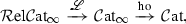
  -enriched \(\infty \)-categories. Following Dwyer–Kan, we define a hammock localization functor from relative \(\infty \)-categories to
  -enriched \(\infty \)-categories, thus providing a rich source of examples of
  -enriched \(\infty \)-categories. Simultaneously unpacking and generalizing one of their key results, we prove that given a relative \(\infty \)-category admitting a homotopical three-arrow calculus, one can explicitly describe the hom-spaces in the \(\infty \)-category presented by its hammock localization in a much more explicit and accessible way. As an application of this framework, we give sufficient conditions for the Rezk nerve of a relative \(\infty \)-category to be a (complete) Segal space, generalizing joint work with Low.
1 Introduction
1.1 Introducing (even more) homotopy theory
In their groundbreaking papers [1, 2], Dwyer–Kan gave the first presentation of the \(\infty \)-category of \(\infty \)-categories, namely the category  of categories enriched in simplicial sets: in modern language, every
  -enriched category has an underlying \(\infty \)-category, and this association induces an equivalence

from the (\(\infty \)-categorical) localization of the category  at the subcategory
  of Dwyer–Kan weak equivalences to the \(\infty \)-category
  of \(\infty \)-categories. Moreover, Dwyer–Kan provided a method of “introducing homotopy theory” into a category
  equipped with a subcategory
  of weak equivalences, namely their hammock localization functor
  of [1].
In this paper, we set up an analogous framework in the setting of \(\infty \)-categories: we prove that the \(\infty \)-category  of \(\infty \)-categories enriched in simplicial spaces likewise models the \(\infty \)-category of \(\infty \)-categories via an equivalence

and we define a hammock localization functor  which likewise provides a method of “introducing (even more) homotopy theory” into relative \(\infty \)-categories. We moreover prove the following two results – the first generalizing a theorem of Dwyer–Kan, the second generalizing joint work with Low (see [5]).
Theorem
(4.4). Given a relative \(\infty \)-category  admitting a homotopical three-arrow calculus, the hom-spaces in the underlying \(\infty \)-category of its hammock localization admit a canonical equivalence

from the groupoid completion of the \(\infty \)-category of three-arrow zigzags  in
in  .
.
Theorem
(6.1). Given a relative \(\infty \)-category  , its Rezk nerve

-
is a Segal space if
 admits a homotopical three-arrow calculus, and
 -
is moreover a complete Segal space if moreover
 is saturated and satisfies the two-out-of-three property.
 admits a homotopical three-arrow calculus, and
 is saturated and satisfies the two-out-of-three property.
(The notion of a homotopical three-arrow calculus is a minor variant on Dwyer–Kan’s “homotopy calculus of fractions” (see Definition 4.1). Meanwhile, the Rezk nerve is a straightforward generalization of Rezk’s “classification diagram” construction, which we introduced in [11] and proved computes the \(\infty \)-categorical localization (see [11, Theorem 3.8 and Corollary 3.12]).)
Remark 1.1
In Remark 2.21, we show how our notion of “ -enriched \(\infty \)-category” fits with the corresponding notion coming from Lurie’s theory of distributors.
Remark 1.2
Many of the original Dwyer–Kan definitions and proofs are quite point-set in nature. However, when working \(\infty \)-categorically, it is essentially impossible to make such ad hoc constructions. Thus, we have no choice but to be both much more careful and much more precise in our generalization of their work.Footnote 1 We find Dwyer–Kan’s facility with universal constructions (displayed in that proof and elsewhere) to be really quite impressive, and we hope that our elaboration on their techniques will be pedagogically useful. Broadly speaking, our main technique is to corepresent higher coherence data.
1.2 Conventions
Though it stands alone, this paper belongs to a series on model \(\infty \)-categories. These papers share many key ideas; thus, rather than have the same results appear repeatedly in multiple places, we have chosen to liberally cross-reference between them. To this end, we introduce the following “code names”.
Title | Reference | Code |
|---|---|---|
Model \(\infty \)-categories I: some pleasant properties of the \(\infty \)-category of simplicial spaces | [10] | S |
The universality of the Rezk nerve | [11] | N |
All about the Grothendieck construction | [12] | G |
Hammocks and fractions in relative \(\infty \)-categories | n/a | H |
Model \(\infty \)-categories II: Quillen adjunctions | [13] | Q |
Model \(\infty \)-categories III: the fundamental theorem | [14] | M |
Thus, for instance, to refer to [10, Theorem 1.9], we will simply write Theorem M.1.9. (The letters are meant to be mnemonical: they stand for “simplicial space”, “nerve”, “Grothendieck”, “hammock”, “Quillen”, and “model”, respectively.)
We take quasicategories as our preferred model for \(\infty \)-categories, and in general we adhere to the notation and terminology of [7, 9]. In fact, our references to these two works will be frequent enough that it will be convenient for us to adopt Lurie’s convention and use the code names T and A for them, respectively.
However, we work invariantly to the greatest possible extent: that is, we primarily work within the \(\infty \)-category of \(\infty \)-categories. Thus, for instance, we will omit all technical uses of the word “essential”, e.g. we will use the term unique in situations where one might otherwise say “essentially unique” (i.e. parametrized by a contractible space). For a full treatment of this philosophy as well as a complete elaboration of our conventions, we refer the interested reader to §S.A. The casual reader should feel free to skip this on a first reading; on the other hand, the careful reader may find it useful to peruse that section before reading the present paper. For the reader’s convenience, we also provide a complete index of the notation that is used throughout this sequence of papers in §S.B.
1.3 Outline
We now provide a more detailed outline of the contents of this paper.
-
In Sect. 2, we introduce the \(\infty \)-category
 of \(\infty \)-categories enriched in simplicial spaces, as well as an auxiliary \(\infty \)-category
  of Segal simplicial spaces. We endow both of these with subcategories of Dwyer–Kan weak equivalences, and prove that the resulting relative \(\infty \)-categories both model the \(\infty \)-category
  of \(\infty \)-categories.
 -
In Sect. 3, we define the \(\infty \)-categories of zigzags in a relative \(\infty \)-category
 between two objects
  , and use these to define the hammock simplicial spaces
  , which will be the hom-simplicial spaces in the hammock localization
  .
. -
In Sect. 4, we define what it means for a relative \(\infty \)-category to admit a homotopical three arrow calculus, and we prove the first of the two results stated above.
-
In Sect. 5, we finally construct the hammock localization functor on relative \(\infty \)-categories, and we explore some of its basic features.
-
In Sect. 6, we prove the second of the two results stated above.
 of
of  of Segal simplicial spaces. We endow both of these with subcategories of Dwyer–Kan weak equivalences, and prove that the resulting relative
  of
of  between two objects
  , and use these to define the hammock simplicial spaces
  , which will be the hom-simplicial spaces in the hammock localization
  .
.2 Segal spaces, Segal simplicial spaces, and  -enriched \(\infty \)-categories
 -enriched
 In this section, we develop the theory—and the homotopy theory—of two closely related flavors of higher categories whose hom-objects lie in the symmetric monoidal \(\infty \)-category  of simplicial spaces equipped with the cartesian symmetric monoidal structure. By “homotopy theory”, we mean that we will endow the \(\infty \)-categories of these objects with relative \(\infty \)-category structures, whose weak equivalences are created by “local” (i.e. hom-object-wise) geometric realization. These therefore constitute “many-object” elaborations on the Kan–Quillen relative \(\infty \)-category
  , whose weak equivalences are created by geometric realization (see Theorem S.4.4). A key source of such objects will be the hammock localization functor, which we will introduce in Sect. 5.
This section is organized as follows.
-
In Sect. 2.1, we recall some basic facts regarding Segal spaces.
-
in Sect. 2.2, we introduce Segal simplicial spaces and define the essential notions for “doing (higher) category theory” with them.
-
In Sect. 2.3, we introduce their full (in fact, coreflective) subcategory of simplicio-spatially-enriched (or simply
 -enriched) \(\infty \)-categories. These are useful since they can more directly be considered as “presentations of \(\infty \)-categories”.
 -
In Sect. 2.4, we prove that freely inverting the Dwyer–Kan weak equivalences among either the Segal simplicial spaces or the
 -enriched \(\infty \)-categories yields an \(\infty \)-category which is canonically equivalent to
  itself. We also contextualize both of these sorts of objects with respect to the theory of enriched \(\infty \)-categories based in the notion of a distributor, and provide some justification for our interest in them.
 -enriched)
  -enriched
  itself. We also contextualize both of these sorts of objects with respect to the theory of enriched
 2.1 Segal spaces
We begin this section with the following recollections. This subsection exists mainly in order to set the stage for the remainder of the section; we refer the reader seeking a more thorough discussion either to the original paper [16] (which uses model categories) or to [8, §1] (which uses \(\infty \)-categories).
Definition 2.1
The \(\infty \)-category of Segal spaces is the full subcategory  of those simplicial spaces satisfying the Segal condition. These sit in a left localization adjunction

which factors the left localization adjunction  of Definition N.2.1 in the sense that we obtain a pair of composable left localization adjunctions

(This follows easily from [16, Theorems 7.1 and 7.2], or alternatively more-or-less follows from [8, Remark 1.2.11].)
In order to make a few basic observations, it will be convenient to first introduce the following.
Definition 2.2
Suppose that  admits finite products. Then, we define the \(\mathbf{0}\)th coskeleton of an object
  (or perhaps more standardly, of the corresponding constant simplicial object
  ) to be the simplicial object selected by the composite

This assembles to a functor
which, as the notation suggests, is given in degree n by \(c \mapsto c^{\times (n+1)}\). This sits in an adjunction

which we refer to as the \(\mathbf{0}\)th coskeleton adjunction for  . Using this, given a simplicial object
  and a map
  in
in  , we define the pullback of Z along \(\varphi \) to be the fiber product

in  , where the vertical map is the component at the object
  of the unit of the 0th coskeleton adjunction. In particular, note that we have a canonical equivalence \((\varphi ^*(Z))_0 \simeq Y\) in
  .
.
Remark 2.3
Suppose that  , and let us write
  for its localization map. Then, the map
  is a surjection in
  , and moreover we have a canonical equivalence
in  . (The first claim follows from [16, Theorem 7.7 and Corollary 6.5], while the second claim follows from combining [8, Definition 1.2.12(b) and Theorem 1.2.13(2)] with the Segal condition for
  .) From here, it follows easily that we have an equivalence

where  denotes the full subcategory on those functors
  that select surjective functors
  . From this viewpoint, the left localization
  is then just the composite functor

where  denotes the \(\infty \)-categorical nerve functor. Thus, one might think of
  as “the \(\infty \)-category of surjectively marked \(\infty \)-categories” (where by “surjectively marked” we mean “equipped with a surjective map from an \(\infty \)-groupoid”).
Remark 2.4
Continuing with the observations of Remark 2.3, note that the category  of strict 1-categories can be recovered as a limit

in  (in which the square is already a pullback). (In fact, the inclusion
  itself fits into the defining pullback square

in  .) We can therefore consider the \(\infty \)-category
  of Segal spaces as a close cousin of the 1-category
  of strict categories, with the caveat that objects of
  must be surjectively marked by a discrete space.
Remark 2.5
Suppose that  . Then, we can compute hom-spaces in the \(\infty \)-category

as follows. Any pair of objects  can be considered as defining a pair of points

Since the map  is a surjection, these admit lifts \(\tilde{x},\tilde{y} \in Y_0\). Then, we have a composite equivalence

by Remarks N.2.2 and 2.3. (In particular, we can compute the hom-space  using any choices of lifts \(\tilde{x},\tilde{y} \in Y_0\).)
2.2 Segal simplicial spaces
We now turn from the  -enriched context to the
  -enriched context.
Definition 2.6
We define the \(\infty \)-category of Segal simplicial spaces to be the full subcategory  of those simplicial objects in
  which satisfy the Segal condition. These sit in a left localization adjunction
  by the adjoint functor theorem (Corollary T.5.5.2.9). We take the convention that our bisimplicial spaces are organized according to the diagram

in  : we think of the columns as the “internal” simplicial spaces, and denote them as
  (omitting the outer index if it’s irrelevant for the discussion). The Segal condition then asserts that the map

is an equivalence in  .
.
Remark 2.7
In light of Remark 2.4, we can consider the \(\infty \)-category  of Segal simplicial spaces as being a homotopical analog of the 1-category
  of simplicial objects in strict 1-categories. The subcategory
  of
of  -enriched categories then corresponds to the full subcategory on those Segal simplicial spaces
  such that the object
  is constant. We will restrict our attention to such objects in Sect. 2.3.
Definition 2.8
For any  , we define the space of objects of
  to be the space

and for any  , we define the hom-simplicial space from x to y in
  to be the pullback

in  . We refer to the points of the space

simply as morphisms from x to y. The various hom-simplicial spaces of  admit associative composition maps

in  , which are obtained as usual via the Segal conditions. For any
  there is an evident identity morphism from x to itself, denoted
  , which behaves as expected under these composition maps.
Definition 2.9
Given any  and any pair of objects
  , we say that two morphisms

are simplicially homotopic if the induced maps
are equivalent (i.e. select points in the same path component of the target). We then say that a morphism  is a simplicial homotopy equivalence if there exists a morphism
  such that the composite morphisms

and

are simplicially homotopic to the respective identity morphisms.
Now, the objects of  will indeed be “presentations of \(\infty \)-categories”, but maps between them which are not equivalences may nevertheless induce equivalences between the \(\infty \)-categories that they present. We therefore introduce the following notion.
Definition 2.10
A map  in
in  is called a Dwyer–Kan weak equivalence if
-
it is weakly fully faithful, i.e. for all pairs of objects
 the induced map
is an equivalence in \(\mathcal {S}\), and
-
it is weakly surjective, i.e. the map
is surjective up to the equivalence relation on
 generated by simplicial homotopy equivalence.
 the induced map

 generated by simplicial homotopy equivalence.
Such morphisms define a subcategory  containing all the equivalences and satisfying the two-out-of-three property, and we denote the resulting relative \(\infty \)-category by
  .
.
Remark 2.11
Via the evident functor  (recall Remark 2.7), the subcategory of Dwyer–Kan weak equivalences
  of Sect. 1.1 (i.e. the subcategory of weak equivalences for the Bergner model structure) is pulled back from the subcategory
  .
.
2.3
 -enriched \(\infty \)-categories
 -enriched
 In light of the discussion of Sect. 2.2, the natural guess for the sense in which a Segal simplicial space should be considered as a “presentation of an \(\infty \)-category” is via the levelwise geometric realization functor

However, this operation does not preserve Segal objects: taking fiber products of simplicial spaces does not generally commute with taking their geometric realizations. On the other hand, these two operations do commute when the common target of the cospan is constant. Hence, it will be convenient to restrict our attention to the following special class of objects.
Definition 2.12
We define the \(\infty \)-category of simplicio-spatially-enriched \(\infty \)-categories, or simply of  -enriched \(\infty \)-categories, to be the full subcategory
  on those objects
  such that
  is constant. We write

for the defining inclusion. Restricting the subcategory  of Dwyer–Kan weak equivalences along this inclusion, we obtain a relative \(\infty \)-category
  (which also has the two-out-of-three property).
Lemma 2.13
There is a canonical factorization

of the restriction of the levelwise geometric realization functor

to the subcategory  of
of  -enriched \(\infty \)-categories.
Proof
Choose any  . Since the functor
  is the inclusion of a full subcategory, it suffices to show that
  , for which in turn it suffices to show that the evident map

is an equivalence. Towards this aim, write
for the decomposition of  into its connected components; since by assumption
  , this induces a decomposition

of  . \(\mathcal {C}_1 \simeq \coprod _i (\mathcal {C}_1)_i\) and \(\mathcal {C}_{n-1} \simeq \coprod _i (\mathcal {C}_{n-1})_i\) for the resulting pulled back decompositions. Then, using Lemma A.5.5.6.17 (applied to the \(\infty \)-topos \(\mathcal {S}\)) and the fact that coproducts commute with connected limits, we can identify the target of the above map as

As  satisfies the Segal condition by assumption, this proves the claim. \(\square \)
Remark 2.14
The proof of Lemma 2.13 shows that it would suffice to make the weaker assumption that the object  is constant in order to conclude that
  .
.
Definition 2.15
We denote simply by

the factorization of Lemma 2.13, and refer to it as the geometric realization functor on  -enriched \(\infty \)-categories.
Definition 2.16
The composite inclusion

clearly factors through the subcategory  . We simply write
for this factorization, and refer to it as the constant  -enriched \(\infty \)-category functor. Thus, for an \(\infty \)-category
  , the simplicial object

is given in degree n by

the constant simplicial space on the object

This functor clearly participates in a commutative diagram

in  .
.
Remark 2.17
Suppose we are given a Segal simplicial space  and a map
  in
in  to its space of objects. Write
  for the corresponding map in
  . Then, the canonical map

is fully faithful (in the  -enriched sense): for any objects
  , the induced map

is already an equivalence in  (instead of just being an equivalence upon geometric realization). Of course, the map
  is therefore in particular weakly fully faithful as well. As we can always choose our original map
  so that the induced map
  is additionally weakly surjective (e.g. by taking \(\varphi \) to be a surjection), it follows that any Segal simplicial space admits a Dwyer–Kan weak equivalence from a
  -enriched category; indeed, we can even arrange to have
  .
.
Improving on Remark 2.17, we now describe a universal way of extracting a  -enriched \(\infty \)-category from a Segal simplicial space.
Definition 2.18
We define the spatialization functor  as follows.Footnote 2 Any
  gives rise to a natural map

in  , the component at
  of the counit of the right localization adjunction
  . The spatialization of
  is then the pullback

(Note that the fiber product of Definition 2.2 that yields this pullback may be equivalently taken either in  or in
or in  , in light of the left localization adjunction of Definition 2.6.) This clearly assembles to a functor, and in fact it is not hard to see that this participates in a right localization adjunction

whose counit components  are Dwyer–Kan weak equivalences (which are even fully faithful as in Remark 2.17).
2.4
 and
and  as presentations of
 and
and  as presentations of
The following pair of results asserts that both  -enriched \(\infty \)-categories and Segal simplicial spaces, equipped with their respective subcategories of Dwyer–Kan weak equivalences, present the \(\infty \)-category of \(\infty \)-categories.
Proposition 2.19
The composite functor

induces an equivalence

Proof
So far, we have obtained the solid diagram

The right adjoint of the composite left localization adjunction

clearly lands in the full subcategory  , and hence restricts to give the right adjoint of a left localization adjunction as indicated by the dotted arrow above. This composes to a left localization adjunction

Moreover, the definition of Dwyer–Kan weak equivalence is precisely chosen so that the composite left adjoint creates the subcategory  [i.e. it is pulled back from the subcategory of equivalences (see Definition N.1.5)]. Hence, by Example N.1.13, it does indeed induce an equivalence

as desired. \(\square \)
Proposition 2.20
Both adjoints in the right localization adjunction

are functors of relative \(\infty \)-categories (with respect to their respective Dwyer–Kan relative structures), and moreover they induce inverse equivalences

in  on localizations.
Proof
The left adjoint inclusion is a functor of relative \(\infty \)-categories by definition. On the other hand, suppose that  is a map in
  . Via the right localization adjunction, its spatialization fits into a commutative diagram

in  , and hence is also in
  by the two-out-of-three property. This shows that the right adjoint is also a functor of relative \(\infty \)-categories.
To see that these adjoints induce inverse equivalences on localizations, note that the composite

is the identity, while the composite

admits a natural weak equivalence in  to the identity functor (namely, the counit of the adjunction). Hence, the claim follows from Lemma N.1.24. \(\square \)
To conclude this section, we make a pair of general remarks regarding  and
and  . We begin by contextualizing these \(\infty \)-categories with respect to Lurie’s theory of enriched \(\infty \)-categories, which is described in [8, §1].
Remark 2.21
Lurie’s theory of enriched \(\infty \)-categories—which provides a satisfactory, compelling, and apparently complete picture (at least when the enriching \(\infty \)-category is equipped with the cartesian symmetric monoidal structure)—is premised on the notion of a distributor, the data of which is simply an \(\infty \)-category  equipped with a full subcategory
  (see [8, Definition 1.2.1]).Footnote 3 Given such a distributor, one can then define \(\infty \)-categories
  and
and  of Segal space objects and of complete Segal space objects with respect to it: these sit as full (in fact, reflective) subcategories

in which
-
the subcategory
 consists of those simplicial objects
  such that
-
\(Y_{\bullet }\) satisfies the Segal condition and
-

-
 consists of those simplicial objects
  such that
(see [8, Definition 1.2.7]), while
-
the subcategory
 consists of those objects which additionally satisfy a certain completeness condition (see [8, Definition 1.2.10]).
 consists of those objects which additionally satisfy a certain completeness condition (see [
Thus,  plays the role of the “enriching \(\infty \)-category”, i.e. the \(\infty \)-category containing the hom-objects in our enriched \(\infty \)-category, while its subcategory
  provides a home for the “object of objects” of the enriched \(\infty \)-category. As in the classical case—indeed, the identity distributor
  simply has
  and
and  —, one can already meaningfully extract an enriched \(\infty \)-category from a Segal space object, but it is only by restricting to the complete ones that one obtains the desired \(\infty \)-category of such.
Now, obviously we have
as Segal simplicial spaces are nothing but Segal space objects with respect to the identity distributor  on the \(\infty \)-category
  of simplicial spaces. We can clearly also identify the \(\infty \)-category of
  -enriched \(\infty \)-categories as

the Segal space objects with respect to the distributor  (the embedding of spaces as the constant simplicial spaces).Footnote 4
\(^,\)
Footnote 5 On the other hand, the subcategory of complete Segal space objects can be identified as the pullback
(the embedding of spaces as the constant simplicial spaces).Footnote 4
\(^,\)
Footnote 5 On the other hand, the subcategory of complete Segal space objects can be identified as the pullback

in which the right vertical functor takes an  -enriched \(\infty \)-category
  to its “levelwise 0th space” object
  .
.
We now explain the source of our interest in the \(\infty \)-categories  and
and  .
.
Remark 2.22
First and foremost, the reason we are interested in  is because this is the natural target of the “pre-hammock localization” functor

whose construction constitutes the main ingredient of the construction of the hammock localization functor itself (see Sect. 5). On the other hand, we then restrict to the (coreflective) subcategory  since this is a convenient full subcategory of
  on which the levelwise geometric realization functor

(which is a colimit) preserves the Segal condition (which is defined in terms of limits) [recall (the proof of) Lemma 2.13].Footnote 6 Indeed, if our “local geometric realization” functor failed to preserve the Segal condition, it would necessarily destroy all “category-ness” inherent in our objects of study. In turn, this would effectively invalidate our right to declare the hammock simplicial spaces

(see Definition 3.17)—which will of course be the hom-simplicial spaces in the hammock localization  —as “presentations of hom-spaces” in any reasonable sense.
For these reasons, Segal simplicial spaces are therefore not really our primary interest. However, since for a Segal simplicial space  , the counit
  of the spatialization right localization adjunction is actually fully faithful in the
  -enriched sense, the hammock localization

will then simultaneously
-
have the hammock simplicial spaces as its hom-simplicial spaces, and
-
have composition maps which both
-
directly present composition in its geometric realization, and
-
manifestly encode the notion of “concatenation of zigzags”.
-
Of course, it would also be possible to restrict further to the (reflective) subcategory

of complete Segal space objects (recall Remark 2.21). However, this is unnecessary for our purposes, since both the pre-hammock localization functor and the hammock localization functor will land in \(\infty \)-categories (namely  and
and  , respectively) which admit canonical relative structures via which they present the \(\infty \)-category
  , thus endowing these constructions with external meaning (which are of course compatible with each other in light of Proposition 2.20). Moreover, as the successive inclusions

respectively admit a left adjoint and a right adjoint, this further restriction would in all probability make for a somewhat messier story.
3 Zigzags and hammocks in relative \(\infty \)-categories
In studying relative 1-categories and their 1-categorical localizations, one is naturally led to study zigzags. Given a relative category  and a pair of objects
  , a zigzag from x to y is a diagram of the form

i.e. a sequence of both forwards and backwards morphisms in  (in arbitrary (finite) quantities and in any order) such that all backwards morphisms lie in
  . Under the 1-categorical localization
  , such a diagram is taken to a sequence of morphisms such that all backwards maps are isomorphisms, so that it is in effect just a sequence of composable (forwards) arrows. Taking their composite, we obtain a single morphism
  in
in  . In fact, one can explicitly construct
  in such a way that all of its morphisms arise from this procedure.
It is a good deal more subtle to show, but in fact the same is true of relative \(\infty \)-categories and their (\(\infty \)-categorical) localizations: given a relative \(\infty \)-category  , it turns out that every morphism in
  can likewise be presented by a zigzag in
  itself. (We prove a precise statement of this assertion as Proposition 3.11.)
The representation of a morphism in  by a zigzag in
  is quite clearly overkill: many different zigzags in
  will present the same morphism in
  . For example, we can consider a zigzag as being selected by a morphism
  of relative \(\infty \)-categories, where
  is a zigzag type which is determined by the shape of the zigzag in question; then, precomposition with a suitable morphism
  of zigzag types will yield a composite
  which presents a canonically equivalent morphism in
  . Thus, in order to obtain a closer approximation to
  , we should take a colimit of the various spaces of zigzags from x to y indexed over the category of zigzag types.
However, this colimit alone will still not generally capture all the redundancy inherent in the representation of morphisms in  by zigzags in
  . Namely, a natural weak equivalence between two zigzags of the same type (which fixes the endpoints) will, upon postcomposing to the localization
  , yield a homotopy between the morphisms presented by the respective zigzags. Pursuing this observation, we are thus led to consider certain \(\infty \)-categories, denoted \({\underline{\mathbf{m }}}(x,y)\) (for varying zigzag types \({\underline{\mathbf{m }}}\)), whose objects are the \({\underline{\mathbf{m }}}\)-shaped zigzags from x to y and whose morphisms are the natural weak equivalences (fixing x and y) between them.
Finally, putting these two observations of redundancy together, we see that in order to approximate the hom-space  , we should be taking a colimit of the various \(\infty \)-categories
  over the category of zigzag types. In fact, rather than taking a colimit of these \(\infty \)-categories, we will take a colimit of their corresponding complete Segal spaces (see §N.2), not within the \(\infty \)-category
  of such but rather within the larger ambient \(\infty \)-category
  in which it is definitionally contained; this, finally, will yield the hammock simplicial space
  , which (as the notation suggests) will be the hom-simplicial space in the hammock localization
  .Footnote 7
This section is organized as follows.
-
In Sect. 3.1, we lay some groundwork regarding doubly-pointed relative \(\infty \)-categories, which will allow us to efficiently corepresent our \(\infty \)-categories of zigzags.
-
In Sect. 3.2, we use this to define \(\infty \)-categories of zigzags in a relative \(\infty \)-category.
-
In Sect. 3.3, we prove a precise articulation of the assertion made above, that all morphisms in the localization
 are represented by zigzags in
  .
. -
In Sect. 3.4, we finally define our hammock simplicial spaces and compare them with the hammock simplicial sets of Dwyer–Kan (in the special case of a relative 1-category).
-
In Sect. 3.5, we assemble some technical results regarding zigzags in relative \(\infty \)-categories which will be useful later; notably, we prove that for a concatenation \([{\underline{\mathbf{m }}} ; {\underline{\mathbf{m }}}']\) of zigzag types, we can recover the \(\infty \)-category \([{\underline{\mathbf{m }}};{\underline{\mathbf{m }}}'] (x,y)\) via the two-sided Grothendieck construction (see Definition G.2.3).
 are represented by zigzags in
  .
.3.1 Doubly-pointed relative \(\infty \)-categories
In this subsection, we make a number of auxiliary definitions which will streamline our discussion throughout the remainder of this paper.
Definition 3.1
A doubly-pointed relative \(\infty \)-category is a relative \(\infty \)-category  equipped with a map
  . The two inclusions
  select objects
  , which we call the source and the target; we will sometimes subscript these to remove ambiguity, e.g. as
  and
and  . These assemble into the evident \(\infty \)-category, which we denote by

Of course, there is a forgetful functor  . We will often implicitly consider a relative \(\infty \)-category
  equipped with two chosen objects
  as a doubly-pointed relative \(\infty \)-category; on the other hand, we may also write
  to be more explicit. We write
  for the full subcategory of doubly-pointed relative categories, i.e. of those doubly-pointed relative \(\infty \)-categories whose underlying \(\infty \)-category is a 1-category.
Notation 3.2
Recall from Notation N.1.6 that  is a cartesian closed symmetric monoidal \(\infty \)-category. With respect to this structure,
  is enriched and tensored over
  . As for the enrichment, for any
  , we define the object

of  (where we write
  and
and  to distinguish between the source and target objects); informally, this should be thought of as the relative \(\infty \)-category whose objects are the doubly-pointed relative functors from
  to
to  , whose morphisms are the doubly-pointed natural transformations between these (i.e. those natural transformations whose components at \(s_1\) and \(t_1\) are
  and
and  , resp.), and whose weak equivalences are the doubly-pointed natural weak equivalences. Then, the tensoring is obtained by taking
  and
and  to the pushout

in  , with its double-pointing given by the natural map from
  . We will write

to denote this tensoring.
Notation 3.3
In order to simultaneously refer to the situations of unpointed and doubly-pointed relative \(\infty \)-categories, we will use the notation  (and similarly for other related notations). When we use this notation, we will mean for the entire statement to be interpreted either in the unpointed context or the doubly-pointed context.
Notation 3.4
We will write

to denote either the tensoring of Notation 3.2 in the doubly-pointed case or else simply the cartesian product in the unpointed case.
3.2 Zigzags in relative \(\infty \)-categories
In this subsection we introduce the first of the two key concepts of this section, namely the \(\infty \)-categories of zigzags in a relative \(\infty \)-category between two given objects.
We begin by defining the objects which will corepresent our \(\infty \)-categories of zigzags.
Definition 3.5
We define a relative word to be a (possibly empty) word \({\underline{\mathbf{m }}}\) in the symbols \(\mathbf{A}\) (for “any arbitrary arrow”) and  . We will write \(\mathbf{A}^{\circ n}\) to denote n consecutive copies of the symbol \(\mathbf{A}\) (for any \(n \ge 0\)), and similarly for
  . We can extract a doubly-pointed relative category from a relative word, which for our sanity we will carry out by reading forwards. So for instance, the relative word
  defines the doubly-pointed relative category

We denote this object by  . Thus, by convention, the empty relative word determines the terminal object
  (which is the unique relative word determining a doubly-pointed relative category whose source and target objects are equivalent). Restricting to the order-preserving maps between relative words (with respect to the evident ordering on their objects, i.e. starting from s and ending at t), we obtain a (non-full) subcategory
  of zigzag types.Footnote 8
\(^{,}\)
Footnote 9
\(^{,}\)
Footnote 10 We will occasionally also use this same relative word notation with the symbol
of zigzag types.Footnote 8
\(^{,}\)
Footnote 9
\(^{,}\)
Footnote 10 We will occasionally also use this same relative word notation with the symbol  , but the resulting doubly-pointed relative categories will not be objects of
  .
.
Remark 3.6
Let  be relative words. Then, their concatenation can be characterized as a pushout

in  (as well as in
  ).
).
Notation 3.7
For any  , we will write
  to denote the number of times that \(\mathbf{A}\) appears in \({\underline{\mathbf{m }}}\), and we will write
  to denote the number of times that
  appears in \({\underline{\mathbf{m }}}\).
Remark 3.8
The localization functor

acts on the subcategory  of zigzag types as

in effect, it collapses all the copies of  and leaves the copies of \([\mathbf{A}]\) untouched.
We now define the first of the two key concepts of this section, an analog of [1, 5.1].
Definition 3.9
Given a relative \(\infty \)-category  equipped with two chosen objects
  , and given a relative word
  , we define the \(\infty \)-category of zigzags in
  from x to y of type \({\underline{\mathbf{m }}}\) to be

If the relative \(\infty \)-category  is clear from context, we will simply write \({\underline{\mathbf{m }}}(x,y)\).
3.3 Representing maps in  by zigzags in
 by zigzags in
In this subsection, we take a digression to illustrate that our study of zigzags in relative \(\infty \)-categories is well-founded: roughly speaking, we show that any morphism in the localization of a relative \(\infty \)-category is represented by a zigzag in the relative \(\infty \)-category itself. We will give the precise assertion as Proposition 3.11. In order to state it, however, we first introduce the following terminology.
Definition 3.10
Let  and
and  be relative \(\infty \)-categories. We will say that a morphism

in  represents the morphism

in  induced by the localization functor. We will also say that it represents the morphism

in  induced from the previous one by the homotopy category functor. In a slight abuse of terminology, we will moreover say that a zigzag

represents the composite

in  , where the map
  is given by \(0 \mapsto 0\) and \(1 \mapsto | {\underline{\mathbf{m }}}|_\mathbf{A}\) (i.e. it corepresents the operation of composition), and likewise for the morphism in the homotopy category
  of the localization selected by either three-fold composite in the commutative diagram

in  .
.
Proposition 3.11
Let  be a relative \(\infty \)-category, and let
  be a functor selecting a morphism in its localization. Then, for some relative word
  , there exists a zigzag
  which represents F.
We will prove Proposition 3.11 in stages of increasing generality. We begin by recalling that any morphism in the 1-categorical localization of a relative 1-category is represented by a zigzag.
Lemma 3.12
Let  be a relative 1-category, and let
  be a functor selecting a morphism in its 1-categorical localization. Then, for some relative word
  , there exists a zigzag
  which represents F.
Proof
This follows directly from the standard construction of the 1-categorical localization of a relative 1-category (see e.g. [1, Proposition 3.1]). \(\square \)
Remark 3.13
Lemma 3.12 accounts for the fundamental role that zigzags play in the theory of relative categories and their 1-categorical localizations. We can therefore view Proposition 3.11 as asserting that zigzags play an analogous fundamental role in the theory of relative \(\infty \)-categories and their (\(\infty \)-categorical) localizations.
Remark 3.14
We can view Lemma 3.12 as guaranteeing the existence of a diagram

for some relative word  , in which
-
the upper dotted arrow is a morphism in
 ,
, -
the lower dotted arrow is its image under the 1-categorical localization functor
and
-
the map
 is as in Definition 3.10.
 ,
,
 is as in Definition
 With Lemma 3.12 recalled, we now move on to the case of \(\infty \)-categorical localizations of relative 1-categories.
Lemma 3.15
Let  be a relative 1-category, and let
  be a functor selecting a morphism in its localization. Then, for some relative word
  , there exists a zigzag
  which represents F.
Proof
Recall from Remark N.1.29 that we have an equivalence  . The resulting postcomposition

of F with the projection to the homotopy category selects a morphism in the 1-categorical localization  . Hence, by Lemma 3.12, we obtain a diagram

for some relative word  , in which
-
the solid horizontal arrows are as in Remark 3.14,
-
the upper map in
 induces the dotted map under the functor
  , so that
 -
the (lower) square in
 commutes.
 induces the dotted map under the functor
  , so that
 commutes.
That the resulting composite

is equivalent to the functor  follows from Lemma 3.16. Thus, in effect, we obtain a diagram

analogous to the one in Remark 3.14 (only with the 1-categorical localizations replaced by the \(\infty \)-categorical localizations), which proves the claim. \(\square \)
Lemma 3.16
For any \(\infty \)-category  and any map
  , the space of lifts

is connected.
Proof
Since the functor  creates the subcategory
  , there is a connected space of lifts of the maximal subgroupoid \(\{ 0 , 1 \} \simeq [1]^\simeq \subset [1]\). Then, in any solid commutative square

there exists a connected space of dotted lifts by definition of the homotopy category. \(\square \)
With Lemma 3.15 in hand, we now proceed to the fully general case of \(\infty \)-categorical localizations of relative \(\infty \)-categories.
Proof of Proposition 3.11
Observe that the morphism  in
in  induces a postcomposition

selecting a morphism in the \(\infty \)-categorical localization of the relative 1-category  . Hence, by Lemma 3.15, we obtain a solid diagram

for some relative word  , in which
-
the lower right diagonal map is an equivalence by Remark N.1.29,
-
we moreover obtain the upper dotted arrow from Remark 3.6 by induction, and
-
we define the lower dotted arrow to be its image under localization.
Now, the resulting composite
fits into a commutative diagram

in  . In particular, we have obtained a lift

of the composite

which must therefore be equivalent to F itself by Lemma 3.16. Thus, we obtain a diagram

as in the proof of Lemma 3.15, which proves the claim. \(\square \)
Thus, zigzags play an important role not just in the theory of relative 1-categories and their 1-categorical localizations, but more generally in the theory of relative \(\infty \)-categories and their \(\infty \)-categorical localizations.
3.4 Hammocks in relative \(\infty \)-categories
For a general relative \(\infty \)-category  , the representation of a morphism in
  by a zigzag
  guaranteed by Proposition 3.11 is clearly far from unique. Indeed, any morphism
  in
in  gives rise to a composite
  which presents the same morphism in
  : in other words, the morphisms in
  corepresent universal equivalence relations between zigzags in relative \(\infty \)-categories (with respect to the morphisms that they represent upon localization).
In order to account for this over-representation, we are led to the following definition, the second of the two key concepts of this section, an analog of [1, 2.1].
Definition 3.17
Suppose  , and suppose
  . We define the simplicial space of hammocks (or alternatively the hammock simplicial space) in
  from x to y to be the colimit

We will extend the hammock simplicial space construction further – and in particular, justify its notation – by constructing the hammock localization

of  in Sect. 5 (see Remark 5.5).
We now compare our hammock simplicial spaces of Definition 3.17 with Dwyer–Kan’s classical hammock simplicial sets (in relative 1-categories).
Remark 3.18
Suppose that  is a relative category. Then, by [1, Proposition 5.5], we have an identification

of the classical simplicial set of hammocks defined in [1, 2.1] as an analogous colimit over the 1-categorical nerves of the (strict) categories of zigzags in  from x to y.Footnote 11 However, there are two reasons that this does not coincide with Definition 3.17.
-
The colimit computing
 is taken in the subcategory
  . This inclusion (being a right adjoint) does not generally commute with colimits.
 -
The functors
 and
and  do not generally agree, but are only related by a natural transformation
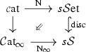
in
 (see Remark N.2.6).
 is taken in the subcategory
  . This inclusion (being a right adjoint) does not generally commute with colimits.
 and
and  do not generally agree, but are only related by a natural transformation
 (see Remark N.2.6).
On the other hand, these two constructions do at least participate in a diagram

in  , which induces a span

in  . We claim that this span lies in the subcategory
  , i.e. that it becomes an equivalence upon geometric realization; as we have a commutative triangle

in  , this will imply that we have a canonical equivalence

in  . We view this as a satisfactory state of affairs, since we are only ultimately interested in simplicial sets/spaces of hammocks as presentations of hom-spaces, anyways.
To see the claim, note first that since  is a left adjoint, it commutes with colimits, and so the left leg of the span lies in
  by the fact that upon postcomposition with the geometric realization functor
  , the natural transformation

in  becomes a natural equivalence

in  (again see Remark N.2.6). By Proposition N.2.4, these geometric realizations of colimits in
  both evaluate to

Now, in order to compute the geometric realization

we begin by observing that the category  has an evident Reedy structure, which one can verify has cofibrant constants, so that the dual Reedy structure on
  has fibrant constants. Moreover, it is not hard to verify that the functor

defines a cofibrant object of  . Hence, the colimit

computes the homotopy colimit in  , i.e. the colimit of the composite

The claim then follows from the string of equivalences

in  (again appealing to Proposition N.2.4).
Remark 3.19
Dwyer–Kan give a point-set definition of the hammock simplicial set in [1, 2.1], and then prove it is isomorphic to the colimit indicated in Remark 3.18. However, working \(\infty \)-categorically, it is essentially impossible to make such an ad hoc definition. Thus, we have simply defined our hammock simplicial space as the colimit to which we would like it to be equivalent anyways.
3.5 Functoriality and gluing for zigzags
In this subsection, we prove that \(\infty \)-categories of zigzags are suitably functorial for weak equivalences among source and target objects (see Notation 3.23), and we use this to give a formula for an \(\infty \)-category of zigzags of type \([{\underline{\mathbf{m }}};{\underline{\mathbf{m }}}']\), the concatenation of two arbitrary relative words  (see Lemma 3.24).
Recall from Remark 3.6 that concatenations of relative words compute pushouts in  . This allows for inductive arguments, in which at each stage we freely adjoin a new morphism along either its source or its target. For these, we will want to have a certain functoriality property for diagrams of this shape. To describe it, let us first work in the special case of
  (instead of
  ). There, if for instance we have an \(\infty \)-category
  with a chosen object
  and we use this to define a new \(\infty \)-category
  as the pushout

then for any target \(\infty \)-category  , the evaluation

will be a cartesian fibration by Corollary T.2.4.7.12 (applied to the functor  ). The following result is then an analog of this observation for relative \(\infty \)-categories; note that there are now two types of “freely adjoined morphisms” we must consider.
Lemma 3.20
Let  , choose any
  , and suppose we are given any
  .
.
-
1.
-
(a)
If we form the pushout
in
 , then the composite restriction
is a cocartesian fibration.
-
(b)
Dually, if we form the pushout
in
 , then the composite restriction
is a cartesian fibration.
-
(a)
-
2.
-
(a)
If we form the pushout
in
 , then the composite restriction
is a cocartesian fibration.
-
(b)
Dually, if we form the pushout
in
 , then the composite restriction
is a cartesian fibration.
-
(a)

 , then the composite restriction

 , then the composite restriction

 , then the composite restriction

 , then the composite restriction
Proof
We first prove item 1(b). Applying Corollary T.2.4.7.12 to the functor

and noting that  (in a way compatible with the evaluation maps), we obtain that the composite restriction

is a cartesian fibration, as desired. The proof of item 1(a) is completely dual.
We now prove item 2(b). For this, consider the diagram

in which all small rectangles are pullbacks and in which we have introduced the ad hoc notation
for the wide subcategory whose morphisms are those natural transformations whose component at  lies in
  . Observing that
  (in a way compatible with the evaluation maps), it follows from applying Corollary T.2.4.7.12 to the functor

that the composite

is a cartesian fibration, for which the cartesian morphisms are precisely those that are sent to equivalences under the restriction functor

Then, by Propositions T.2.4.2.3(2) and T.2.4.1.3(2), the functor

is also a cartesian fibration, for which any morphism that is sent to an equivalence under the composite

is cartesian. Now, for any map  in
in  and any object

choose such a cartesian morphism

Since by definition  , it follows that this is in fact a morphism in the (wide) subcategory
  . Hence, we obtain a diagram

in  , in which the right square is a pullback since \(\tilde{\varphi }\) is a cartesian morphism. Moreover, again using the fact that
  , it is easy to check that the left square is also a pullback. So the entire rectangle is a pullback, and hence \(\tilde{\varphi }\) is also a cartesian morphism for the functor

From here, it follows from the fact that  is a subcategory that this functor is indeed a cartesian fibration. The proof of item 2(a) is completely dual. \(\square \)
Given an arbitrary doubly-pointed relative \(\infty \)-category  and some relative \(\infty \)-category
  which we consider to be doubly-pointed via some choice
  of a pair of objects, we will be interested in the functoriality of the construction

in the variable  but for a fixed choice of
  (or vice versa). This functoriality will be expressed by a variant of Lemma 3.20. However, in order to accommodate the fixing of just one of the two chosen objects, we must first introduce the following notation.
Notation 3.21
Let  , let
, let  , and let
  . Then, we write

and

We now give a “half-doubly-pointed” variant of Lemma 3.20, but stated only in the special case that we will need.
Lemma 3.22
Let  , let
, let  , and let

-
1.
The functor

-
(a)
is a cocartesian fibration if \({\underline{\mathbf{m }}}\) begins with
 , and
, and -
(b)
is a cartesian fibration if \({\underline{\mathbf{m }}}\) begins with \(\mathbf{A}\).
-
(a)
-
2.
The functor

-
(a)
is a cartesian fibration if \({\underline{\mathbf{m }}}\) ends with
 , and
, and -
(b)
is a cocartesian fibration if \({\underline{\mathbf{m }}}\) ends with \(\mathbf{A}\).
-
(a)

 , and
, and
 , and
, andProof
If we simply have \({\underline{\mathbf{m }}} = [\mathbf{A}]\) or  then these statements follow trivially from Lemma 3.20, so let us assume that the relative word \({\underline{\mathbf{m }}}\) has length greater than 1.
To prove item 2(a), suppose that  . Then we have a pullback square

which, making the identification of  with
with  in a way which switches the source and target objects, is equivalently a pullback square

From here, the proof parallels that of Lemma 3.20(1)(b), only now we apply Corollary T.2.4.7.12 to the functor

The proof of item 1(a) is completely dual.
To prove item 1(b), let us now suppose that \({\underline{\mathbf{m }}} = [\mathbf{A};{\underline{\mathbf{m }}}']\). Then we have a diagram

in which all small rectangles are pullbacks, almost identical to that of the proof of Lemma 3.20(2)(b). From here, the proof proceeds in a completely analogous way to that one. The proof of item 2(b) is completely dual. \(\square \)
Lemma 3.22, in turn, enables us to make the following definitions.
Notation 3.23
Let  , let
, let  , and let
  .
.
-
If \({\underline{\mathbf{m }}}\) begins with
 , we write
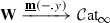
for the functor classifying the cocartesian fibration of Lemma 3.22(1)(a). On the other hand, if \({\underline{\mathbf{m }}}\) begins with \(\mathbf{A}\), we write
for the functor classifying the cartesian fibration of Lemma 3.22(1)(b).
-
If \({\underline{\mathbf{m }}}\) ends with
 , we write
for the functor classifying the cartesian fibration of Lemma 3.22(2)(a). On the other hand, if \({\underline{\mathbf{m }}}\) ends with \(\mathbf{A}\), we write
for the functor classifying the cocartesian fibration of Lemma 3.22(2)(b).
-
By convention and for convenience, if
 is the empty relative word (which defines the terminal relative \(\infty \)-category), we let both \({\underline{\mathbf{m }}}(x,-)\) and \({\underline{\mathbf{m }}}(-,y)\) denote either functor
or
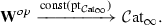
 , we write

 , we write

 is the empty relative word (which defines the terminal relative

Using Notation 3.23, we now express the \(\infty \)-category  of zigzags in
  from x to y of the concatenated zigzag type
  in terms of the two-sided Grothendieck construction (see Definition G.2.3). This is an analog of [1, 9.4].Footnote 12
Lemma 3.24
Let  . Then for any
  and any
  , we have an equivalence

which is natural in  .
.
Proof
Recall from Remark 3.6 that we have a pushout square

in  , through which \([{\underline{\mathbf{m }}};{\underline{\mathbf{m }}}']\) acquires its source object from \({\underline{\mathbf{m }}}\) and its target object from \({\underline{\mathbf{m }}}'\). This gives rise to a string of equivalences

in  . From here, the first and second cases follow from Lemma 3.22, Notation 3.23, and Definition G.2.3, while the third and fourth cases follow by additionally appealing to Example G.1.9 and Example G.2.3. \(\square \)
4 Homotopical three-arrow calculi in relative \(\infty \)-categories
In the previous section, given a relative \(\infty \)-category  , we introduced the hammock simplicial space

for two objects  . The definition of this simplicial space is fairly explicit, but it is nevertheless quite large. In this section, we show that under a certain condition—namely, that
  admits a homotopical three-arrow calculus—we can at least recover this simplicial space up to weak equivalence in
  (i.e. we can recover its geometric realization) from a much smaller simplicial space, in fact from one of the constituent simplicial spaces in its defining colimit. This condition is often satisfied in practice; for example, it holds when
  admits the additional structure of a model \(\infty \)-category (see Lemma M.8.2).
This section is organized as follows.
-
In Sect. 4.1, we define what it means for a relative \(\infty \)-category to admit a homotopical three-arrow calculus, and we state the fundamental theorem of homotopical three-arrow calculi (Theorem 4.4) described above.
-
In Sect. 4.2, in preparation for the proof of Theorem 4.4, we assemble some auxiliary results regarding relative \(\infty \)-categories.
-
In Sect. 4.3, in preparation for the proof of Theorem 4.4, we assemble some auxiliary results regarding ends and coends.
4.1 The fundamental theorem of homotopical three-arrow calculi
We begin with the main definition of this section, whose terminology will be justified by Theorem 4.4; it is a straightforward generalization of [5, Definition 4.1], which is itself a minor variant of [1, 6.1(i)].
Definition 4.1
Let  . We say that
  admits a homotopical three-arrow calculus if for all
  and for all \(i,j \ge 1\), the map

in  obtained by collapsing the middle weak equivalence induces a map

in  (i.e. it becomes an equivalence upon applying the groupoid completion functor
  ).
).
Notation 4.2
Since it will appear repeatedly, we make the abbreviation  for the relative word

Definition 4.3
For any relative \(\infty \)-category  and any objects
  , we will refer to

as the \(\infty \)-category of three-arrow zigzags in  from x to y.
We now state the fundamental theorem of homotopical three-arrow calculi, an analog of [1, Proposition 6.2(i)]; we will give its proof in Sect. 4.4.
Theorem 4.4
If  admits a homotopical three-arrow calculus, then for any
  , the natural map

in  becomes an equivalence under the geometric realization functor
  .
.
4.2 Supporting material: relative \(\infty \)-categories
In this subsection, we give two results regarding relative \(\infty \)-categories which will be used in the proof of Theorem 4.4. Both concern corepresentation, namely the effect of the functor

on certain data in  (for a given relative \(\infty \)-category
  ).
).
Lemma 4.5
Given a pair of maps  in
in  , a morphism between them in
  induces, for any
  , a natural transformation between the two induced functors

Proof
First of all, the morphism in  is selected by a map
  ; this is equivalent to a map

in  , which is adjoint to a map

in  . Then, for any
  , composing with this map yields a functor

which is adjoint to a map

which selects a natural transformation between the two induced functors

as desired. \(\square \)
Lemma 4.6
Let  , and form any pushout diagram

in  , where the left map is the unique map in
  . Note that the two possible retractions
  in
in  of the given map induce retractions
  in
in  . Then, for any
  , the induced map

becomes an equivalence under the functor  , with inverse given by either map

in  induced by one of the given retractions.
Proof
Note that both composites

(of one of the two possible retractions followed by the given map) are connected to  by a map in

In turn, both composites

are connected to  by a map in
  . Hence, the result follows from Lemmas 4.5 and N.1.26. \(\square \)
4.3 Supporting material: co/ends
In this subsection, we give a few results regarding ends and coends which will be used in the proof of Theorem 4.4. For a brief review of these universal constructions in the \(\infty \)-categorical setting, we refer the reader to [3, §2].
We begin by recalling a formula for the space of natural transformations between two functors.
Lemma 4.7
Given any  and any
  , we have a canonical equivalence

Proof
This appears as [4, Proposition 2.3] (and as [3, Proposition 5.1]). \(\square \)
We now prove a “ninja Yoneda lemma”.Footnote 13
Lemma 4.8
If  is an \(\infty \)-category equipped with a tensoring
  , then for any functor
  , we have an equivalence

in  .
.
Proof
For any test objects  and
and  , we have a string of natural equivalences

where the first line follows from the definition of a coend as a colimit (see e.g. [3, Definition 2.5]), the second line uses the tensoring, the third line follows from Lemma 4.7, and the last line follows from the usual Yoneda lemma (Proposition T.5.1.3.1). Hence, again by the Yoneda lemma, we obtain an equivalence

which is natural in  . \(\square \)
Then, we have the following result on the preservation of colimits.Footnote 14
Lemma 4.9
If  is an \(\infty \)-category equipped with a tensoring
  , then for any functor
  , the functor

is a left adjoint.
Proof
It suffices to check that for every  , the functor

is representable. For this, given any  we compute that

where the first line follows from the definition of a co/end as a co/limit (again see e.g. [3, Definition 2.5]), the second line uses the tensoring, and the last line follows from Lemma 4.7. \(\square \)
4.4 The proof of Theorem 4.4
Having laid out the necessary supporting material in the previous two subsection, we now proceed to prove the fundamental theorem of homotopical three-arrow calculi (Theorem 4.4). This proof is based closely on that of [1, Proposition 6.2(i)], although we give many more details (recall Remark 1.2).
Proof of Theorem 4.4
We will construct a commutative diagram

in  , i.e. a commutative square in which the bottom arrow is equipped with a retraction and in which moreover the top and right map are equivalences. Note that by definition, the object on the bottom left is precisely
  ; the left map will be the natural map referred to in the statement of the result. The equivalences in
  satisfy the two-out-of-six property, and applying this to the composable sequence of arrows
  , we deduce that \(|\alpha |\) is also an equivalence, proving the claim.
We will accomplish this by running through the following sequence of tasks.
-
1.
Define the two objects on the right.
-
2.
Define the maps in the diagram.
-
3.
Explain why the square commutes.
-
4.
Explain why \(|\rho |\) gives a retraction of
 .
. -
5.
Explain why the map \(|\beta |\) is an equivalence.
-
6.
Explain why the map
 is an equivalence.
 .
. is an equivalence.
We now proceed to accomplish these tasks in order.
-
1.
We define endofunctors
 by the formulas
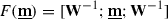
and

Then, the object in the upper right is given by
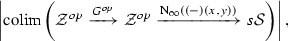
and the object in the bottom right is given by
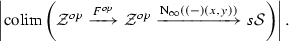
-
2.
We define the two evident natural transformations
 (given by collapsing the two newly added copies of
  ) and
) and  (given by collapsing all internal copies of
  ) in
) in  ; these induce natural transformations
  and
and  in
in  .Footnote 15 We then define the maps in the diagram as follows.
-
The left map is obtained by taking the geometric realization of the inclusion

into the colimit at the object
 .
. -
The top map is obtained by taking the geometric realization of the inclusion

into the colimit at the object
 . (Note that
  in
in  .)
.) -
The right map is obtained by taking the geometric realization of the map

on colimits induced by the natural transformation
 in
in  .
. -
The bottom map in the square (i.e. the straight bottom map) is obtained by taking the geometric realization of the map
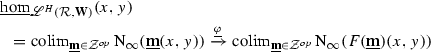
on colimits induced by the natural transformation
 in
in  .
. -
The curved map is obtained by taking the geometric realization of the map
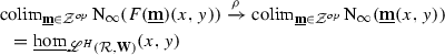
on colimits induced by the functor

-
-
3.
The upper composite in the square is given by the geometric realization of the composite
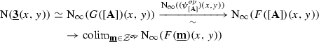
of the equivalence induced by the component of
 at the object
  (which is an isomorphism in
  ) followed by the inclusion into the colimit at \([\mathbf{A}]\). So, via the (unique) identification \({\underline{\mathbf{3 }}} \cong F([\mathbf{A}])\), we can identify this composite with the inclusion into the colimit at
  . Meanwhile, the lower composite in the square is given by the geometric realization of the composite
of the map induced by the component of \(\varphi ^{op}\) at \({\underline{\mathbf{3 }}}\) followed by the inclusion into the colimit at \({\underline{\mathbf{3 }}}\). Now, the map
 in
in  is given by
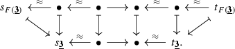
On the other hand, applying F to the unique map
 in
in  , we obtain a map
  in
in  given by
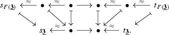
which corepresents a map

in
 which participates in the diagram
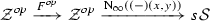
defining
 . So, in order to witness the commutativity of the square, it suffices to obtain an equivalence between the two maps
But there is an evident cospan in
 between the two maps \(\varphi _{\underline{\mathbf{3 }}}\) and \(F(\gamma )\), so this follows from Lemma 4.5, Lemma N.1.26, and Proposition N.2.4.
 -
4.
The fact that
 follows from applying Proposition G.2.5 to the diagram
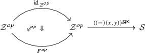
and invoking Proposition N.2.4 to obtain a retraction diagram
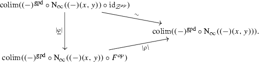
-
5.
We first claim that for any
 , the map
is an isomorphism. Indeed, note that by Proposition G.2.1, we have an equivalence

The category
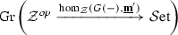
admits a span of natural transformations from the identity functor to its fiber over the object
 , whose component at an object
  is indicated by the natural commutative diagram
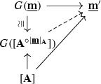
in
 (in which the dotted arrow is simply the extension of the upper map over an isomorphism).Footnote 16 Hence, by Lemma N.1.26 the inclusion of the fiber over
  induces an equivalence upon groupoid completions. But this fiber is precisely
  .
.
 by the formulas


 (given by collapsing the two newly added copies of
  ) and
) and  (given by collapsing all internal copies of
  ) in
) in  ; these induce natural transformations
  and
and  in
in  .
.
 .
.
 . (Note that
  in
in  .)
.)
 in
in  .
.
 in
in  .
.


 at the object
  (which is an isomorphism in
  ) followed by the inclusion into the colimit at
  . Meanwhile, the lower composite in the square is given by the geometric realization of the composite
 in
in  is given by
 in
in  , we obtain a map
  in
in  given by

 which participates in the diagram
 . So, in order to witness the commutativity of the square, it suffices to obtain an equivalence between the two maps
 between the two maps
  follows from applying Proposition G.2.5 to the diagram

 , the map


 , whose component at an object
  is indicated by the natural commutative diagram
 (in which the dotted arrow is simply the extension of the upper map over an isomorphism).
 induces an equivalence upon groupoid completions. But this fiber is precisely
  .
.Now, assembling the above observation over all  , we see that the map

is an equivalence in  . Using this, and denoting by
  the evident tensoring

we obtain the map

as string of equivalences

in  , in which
-
the second and fifth lines are purely for notational convenience,
-
we apply to the functor
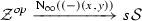
-
Lemma 4.8 to obtain the first line,
-
Lemma 4.9 to obtain the fourth line, and
-
Lemma 4.8 again to obtain the last line,
and
-
-
the third line follows from the equivalence in
 obtained above.

 obtained above.
(So in fact, the map \(\beta \) itself is already an equivalence in  (i.e. before geometric realization).)
-
6.
We claim that for every
 the map
in
 becomes an equivalence after geometric realization. This follows from an analysis of the corepresenting map
  in
in  : it can be obtained as a composite
in
 , in which each \({\underline{\mathbf{m }}}'_i\) is obtained from \({\underline{\mathbf{m }}}'_{i-1}\) by omitting one of the internal appearances of
  in \(F({\underline{\mathbf{m }}})\), and the corresponding map
  is obtained by collapsing this copy of
  to an identity map. Each map
in
 becomes an equivalence after geometric realization, by Lemma 4.6 when the about-to-be-omitted appearance of
  in \({\underline{\mathbf{m }}}'_{i-1}\) is adjacent to another appearance of
  , and by applying the definition of
  admitting a homotopical three-arrow calculus (Definition 4.1) to (either one or two iterations, depending on the shape of \({\underline{\mathbf{m }}}'_{i-1}\), of) the combination of Lemma 3.24 and Proposition G.2.4. Hence, the composite map
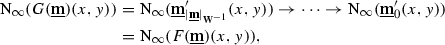
which is precisely the map
 , does indeed become an equivalence upon geometric realization as well. Then, since colimits commute, it follows that the induced map
is an equivalence in
 . \(\square \)
 the map
 becomes an equivalence after geometric realization. This follows from an analysis of the corepresenting map
  in
in  : it can be obtained as a composite
 , in which each
  in
in  is obtained by collapsing this copy of
  to an identity map. Each map
 becomes an equivalence after geometric realization, by Lemma
  in
in  , and by applying the definition of
  admitting a homotopical three-arrow calculus (Definition
 , does indeed become an equivalence upon geometric realization as well. Then, since colimits commute, it follows that the induced map
 .
. 5 Hammock localizations of relative \(\infty \)-categories
In Sect. 3, given a relative \(\infty \)-category  and a pair of objects
  , we defined the corresponding hammock simplicial space

(see Definition 3.17). In this section, we proceed to globalize this construction, assembling the various hammock simplicial spaces of  into a Segal simplicial space—and thence a
  -enriched \(\infty \)-category—whose compositions encode the concatenation of zigzags in
  .
.
The bulk of the construction of the hammock localization consists in constructing the pre-hammock localization: this will be a Segal simplicial space

whose nth level is given by the colimit

For clarity, we proceed in stages.
First, we build an object which simultaneously corepresents
-
all possible sequences (of any length) of composable zigzags, and
-
all possible concatenations among these sequences.
Construction 5.1
Observe that  is a monoid object, i.e. a monoidal category: its multiplication is given by the concatenation functor

and the unit map  selects the terminal object
  .Footnote 17 We can thus define its bar construction

which has  (so that
  ), with face maps given by concatenation and with degeneracy maps given by the unit. This admits an oplax natural transformation to the functor

which we encode as a commutative triangle

in  (recall Definition G.3.1 and Example G.1.15): in simplicial degree n, this is given by the iterated concatenation functor

(which in degree 0 is simply the composite

i.e. the inclusion of the terminal object  ).Footnote 18
\(^,\)
Footnote 19 Taking opposites, we obtain a commutative triangle
).Footnote 18
\(^,\)
Footnote 19 Taking opposites, we obtain a commutative triangle

in  , which now encodes a lax natural transformation from the bar construction

on the monoid object  (note that the involution
  is covariant) to the functor

We now map into an arbitrary relative \(\infty \)-category and extract the indicated colimits, all in a functorial way.
Construction 5.2
A relative \(\infty \)-category  represents a composite functor

Considering this as a natural transformation  in
in  , we can postcompose it with the lax natural transformation obtained in Construction 5.1, yielding a composite lax natural transformation encoded by the diagram

in  . Then, by Proposition T.4.2.2.7, there is a unique “fiberwise colimit” lift in the diagram

in  .Footnote 20 Thus, the resulting composite

takes each object  to the colimit of the composite

We denote this simplicial object in simplicial spaces by

Allowing  to vary, this assembles into a functor

We now show that the bisimplicial spaces of Construction 5.2 are in fact Segal simplicial spaces.
Lemma 5.3
For any  , the object
  satisfies the Segal condition.
Proof
We must show that for every \(n \ge 2\), the nth Segal map

(to the n-fold fiber product) is an equivalence in  . As
. As  is an \(\infty \)-topos, colimits therein are universal, i.e. they commute with pullbacks [see Definition T.6.1.0.4 and Theorem T.6.1.0.6 (and the discussion at the beginning of §T.6.1.1)]. Moreover, note that we have a canonical equivalence
  in
in  . Hence, by induction, we have a string of equivalences

(where in the penultimate line we appeal to Fubini’s theorem for colimits) which, chasing through the definitions, visibly coincides with the nth Segal map. This proves the claim. \(\square \)
We finally come to the main point of this section.
Definition 5.4
By Lemma 5.3, the functor given in Construction 5.2 admits a factorization

through the \(\infty \)-category of Segal simplicial spaces. We again denote this factorization by

and refer to it as the pre-hammock localization functor.Footnote 21 Then, we define the hammock localization functor

to be the composite

Remark 5.5
Given a relative \(\infty \)-category  , the 0th level of its pre-hammock localization

is given by

which is simply the nerve  of the subcategory
  of weak equivalences. Thus, its space of objects is simply

Moreover, unwinding the definitions, it is manifestly clear that
-
its hom-simplicial spaces are precisely the hammock simplicial spaces of
 (recall Definitions 2.8 and 3.17), and
 -
its compositions correspond to concatenation of zigzags (with identity morphisms corresponding to zigzags of type
 ).
).
 (recall Definitions
  ).
).Of course, we have a canonical counit weak equivalence

in  which is even fully faithful in the
  -enriched sense, so that the hammock localization enjoys all these same properties.
Just as in the 1-categorical case, the hammock localization of  admits a natural map from
  .
.
Construction 5.6
Returning to Construction 5.1, observe that there is a tautological section

which takes  to
to  , and which takes a map
  in
in  to the map corresponding to the fiber map which, in the ith factor of
  , is given by the unique map

in  . This is opposite to a tautological section

which gives rise to a composite map

admitting a natural transformation to the standard inclusion (as the “target” factor, i.e. the fiber over \(1 \in [1]\)). This postcomposes with the composite

appearing in Construction 5.2 to give a natural transformation

in  .Footnote 22 Thus, in simplicial degree n, this map is simply the inclusion into the colimit defining
  at the object

Restricting levelwise to (the nerve of) the maximal subgroupoid, we obtain a composite

As this source lies in  , we obtain a canonical factorization

in  . This clearly assembles into a natural transformation

in  .
.
Definition 5.7
For a relative \(\infty \)-category  , we refer to the map

in  of Construction 5.6 as its tautological inclusion.
We end this section with the following fundamental result, an analog of [1, Proposition 3.3]. In essence, it shows that when considered as morphisms in the hammock localization, weak equivalences in  both represent and corepresent equivalences in the underlying \(\infty \)-category. Just as with the fundamental theorem of homotopical three-arrow calculi (Theorem 4.4), its proof will be substantially more involved than that of its 1-categorical analog (recall Remark 1.2).
Proposition 5.8
Let  , and let
  . Suppose we are given a weak equivalence

and let us also denote by  the resulting composite morphism

Then, the induced “composition with w” maps

and

in  become equivalences in
  upon geometric realization. Moreover, if we denote by
  the composite morphism

then their inverses are respectively given by the geometric realizations of the induced “composition with \(w^{-1}\)” maps

and

in  .
.
Proof
We prove the first statement; the second statement follows by a nearly identical argument. Moreover, we will only show that the composite map

is an equivalence; that the composite

is an equivalence will follow from a very similar argument.
For each  , let us define a functor

given informally by taking a zigzag

in  to the zigzag

in  , in which both new maps are the chosen weak equivalence w.Footnote 23 This operation is clearly natural in
  , i.e. it assembles into a natural transformation

Then, using Proposition N.2.4 and the fact that the geometric realization functor  commutes with colimits (being a left adjoint), we see that the composite

is obtained as the composite

To see that this is an equivalence, for each  let us define a map
  in
in  to be opposite the map
  in
in  which collapses the newly concatenated copy of
  to the map
  . These assemble into a natural transformation
  in
in  , and hence we obtain a natural transformation

Moreover, For each  we have a functor

adjoint to a functor

given informally by taking a zigzag

in  to the diagram

in  representing a morphism in
  , where the maps in the right two squares are all either the chosen weak equivalence
  or are
  . These assemble into a morphism

in  , i.e. a modification from
  to \(\varphi \). By Proposition G.2.8, this induces a natural transformation

which, by Lemma N.1.26 and Proposition G.2.1, gives a homotopy between the maps

and

in  . Hence, to show that the above composite is an equivalence, it suffices to show that the composite

is an equivalence. But this composite fits into a commutative triangle

obtained by applying Proposition G.2.5 to the diagram

so it is an equivalence. This proves the claim. \(\square \)
6 From fractions to complete Segal spaces, redux
As an application of the theory developed in this paper, we now provide a sufficient condition for the Rezk nerve  of a relative \(\infty \)-category
  to be either
-
a Segal space or
-
a complete Segal space,
thus giving a partial answer to our own Question N.3.6, which we refer to as the calculus theorem.Footnote 24 This result is itself a direct generalization of joint work with Low regarding relative 1-categories (see [5, Theorem 4.11]). That result, in turn, generalizes work of Rezk, Bergner, and Barwick–Kan; we refer the reader to [5, §1] for a more thorough history.
Theorem 6.1
Suppose that  admits a homotopical three-arrow calculus.
-
1.
 is a Segal space.
 -
2.
Suppose moreover that
 satisfies the two-out-of-three property. Then
  is a complete Segal space if and only if
  is saturated.
 is a Segal space.
 satisfies the two-out-of-three property. Then
  is a complete Segal space if and only if
  is saturated.
The proof of the calculus theorem (Theorem 6.1) is very closely patterned on the proof of [5, Theorem 4.11] (the main theorem of that paper), which is almost completely analogous but holds only for relative 1-categories.Footnote 25 We encourage any reader who would like to understand it to first read that paper: there are no truly new ideas here, only generalizations from 1-categories to \(\infty \)-categories.
Proof of Theorem 6.1
For this proof, we give a detailed step-by-step explanation of what must be changed in the paper [5] to generalize its main theorem from relative 1-categories to relative \(\infty \)-categories.
-
For [5, Definition 2.1], we replace the notion of a “weak homotopy equivalence” of categories by the notion of a map in
 which becomes an equivalence under
  (i.e. a Thomason weak equivalence (see Definition G.A.2 and Remark G.A.3)).
 -
The proof of [5, Lemma 2.2] carries over easily using Lemma N.1.26.
-
For [5, Definition 2.3], we replace the notion of a “homotopy pullback diagram” of categories by the notion of a commutative square in
 which becomes a pullback square under
  (i.e. a homotopy pullback diagram in
  ).
). -
For [5, Definition 2.4], we replace the notions of “Grothendieck fibrations” and “Grothendieck opfibrations” of categories by those of cartesian fibrations and cocartesian fibrations of \(\infty \)-categories (see §G.1 and [15]).
-
For [5, Remark 2.5], as the entire theory of \(\infty \)-categories is in essence already only pseudofunctorial, there is no corresponding notion of a co/cartesian fibration being “split” (or rather, every co/cartesian fibration should be thought of as being “split”).
-
The evident generalization of [5, Example 2.6] can be obtained by applying Corollary T.2.4.7.12 to an identity functor of \(\infty \)-categories.
-
The evident generalization of (the first of the two dual statements of) [5, Theorem 2.7] is proved as Corollary G.4.3.
-
The evident generalization of [5, Corollary 2.8] again follows directly (or can alternatively be obtained by combining Example N.1.12 and Lemma N.1.20).
-
For [5, Definition 2.9], we use the definition of the “two-sided Grothendieck construction” given in Definition G.2.3. (Note that the 1-categorical version is simply the corresponding (strict) fiber product.)
-
The evident analog of [5, Lemma 2.11] is proved as Proposition G.2.4.
-
For [5, Definition 3.1], we replace the notion of a “relative category” by the notion of a “relative \(\infty \)-category” given in Definition N.1.1; recall from Remark N.1.2 that here we are actually working with a slightly weaker definition. We replace the notion of its “homotopy category” by that of its localization given in Definition N.1.8. We have already defined the notion of a relative \(\infty \)-category being “saturated” in Definition N.1.14.
-
For [5, Definition 3.2], we have already made the analogous definitions in Notation N.1.6.
-
For [5, Definitions 3.3 and 3.6], we have already made the analogous definitions in Definitions 3.5 and 3.9.
-
The evident analog of [5, Remark 3.7] is now true by definition (recall Notation 3.2).
-
For [5, Proposition 3.8], the paper actually only uses part (ii), whose evident analog is provided by Lemma 3.20(1).
-
For [5, Lemma 3.10], note that the functors in the statement of the result as well as in its proof are all corepresented by maps in
 ; the proof of the analogous result thus carries over by Lemma 4.5.
 -
For [5, Lemma 3.11], again everything in the statement of the result as well as in its proof are all corepresented; again the proof carries over by Lemma 4.5.
-
For [5, Definition 4.1], we have already defined a “homotopical three-arrow calculus” for a relative \(\infty \)-category in Definition 4.1.
-
For [5, Theorem 4.5], we use the more general but slightly different definition of hammocks given in Definition 3.17 (recall Remark 3.18); part (i) is proved as Theorem 4.4, while part (ii) follows immediately from the definitions, particularly Definitions 5.4 and 2.8. (Note that in the present framework, the “reduction map” is simply replaced by the canonical map to the colimit defining the simplicial space of hammocks.)
-
For [5, Corollary 4.7], the evident analog of [1, Proposition 3.3] is proved as Proposition 5.8.
-
For [5, Proposition 4.8], the proof carries over essentially without change. (The functor considered there when proving that the rectangle (AC) is a homotopy pullback diagram is replaced by our functor
 of Notation 3.23.)
 -
For [5, Lemma 4.9], the map itself in the statement of the result comes from the functoriality
and
of Notation 3.23, as do the vertical maps in the commutative square in the proof. The horizontal maps in that square are corepresented by maps in
 , and it clearly commutes by construction. The evident analog of [1, Proposition 9.4] is proved as Lemma 3.24.
 -
For [5, Proposition 4.10], note that all morphisms in both the statement of the result and its proof are corepresented by maps in
 ; the proof itself carries over without change.
 -
For [5, Theorem 4.11] (whose analog is Theorem 6.1 itself), note that we are now proving an \(\infty \)-categorical statement (instead of a model-categorical one), and so there are no issues with fibrant replacement.
-
The proof of part (1) of Theorem 6.1 is identical to the proof of part (i) there: it follows from our analog of [5, Proposition 4.10].
-
We address the two halves of the proof of part (2) of Theorem 6.1 in turn.
- \(*\) :
-
The proof of the “only if” direction runs analogously to that of [5, Theorem 4.11(ii)], only now we use that given two objects
 in an \(\infty \)-category
  , any path between their postcompositions
  can be represented by a zigzag
  connecting them (for some sufficiently large i).
 - \(*\) :
-
We must modify the proof of the “if” direction slightly, as follows. Assume that
 is saturated. By the local universal property of the Rezk nerve (Theorem N.3.8), we have an equivalence
  in
in  . Note also that by the two-out-of-three assumption, any two objects
  which select the same path component under the composite
are either both weak equivalences or both not weak equivalences. Now, for any object of
 , recalling Remark 2.3 and invoking the saturation assumption, we see that the corresponding map
  selects an equivalence under the postcomposition
  if and only if it factors as
  . From here, the proof proceeds identically. \(\square \)
-
 which becomes an equivalence under
  (i.e. a Thomason weak equivalence (see Definition G.A.2 and Remark G.A.3)).
 which becomes a pullback square under
  (i.e. a homotopy pullback diagram in
  ).
). ; the proof of the analogous result thus carries over by Lemma
  of Notation

 , and it clearly commutes by construction. The evident analog of [
 ; the proof itself carries over without change.
 in an
in an  , any path between their postcompositions
  can be represented by a zigzag
  connecting them (for some sufficiently large i).
 is saturated. By the local universal property of the Rezk nerve (Theorem N.3.8), we have an equivalence
  in
in  . Note also that by the two-out-of-three assumption, any two objects
  which select the same path component under the composite
 , recalling Remark
  selects an equivalence under the postcomposition
  if and only if it factors as
  . From here, the proof proceeds identically.
 Remark 6.2
After establishing the necessary facts concerning model \(\infty \)-categories, we obtain an analog of [5, Corollary 4.12] as Theorem M.10.1.
Remark 6.3
In light of Remark N.3.2, [5, Remark 4.13] is strictly generalized by the local universal property of the Rezk nerve (Theorem N.3.8).
Notes
The word “spatialization” is meant to indicate that the 0th object of its output will lie in the subcategory
 of constant simplicial spaces.
To see that the inclusion
 of the full subcategory of constant objects is a distributor, note that if
  is an \(\infty \)-topos and
  is a full subcategory which is stable under limits and colimits, then
  is automatically a distributor. The only remaining point is to verify condition (4) of [8, Definition 1.2.1]. The functor
  is given on objects by
  , with functoriality given by pullback in
  . This clearly factors as the composite
  , in which the latter functor is similarly given by
  , which then preserves colimits by Proposition T.6.1.3.10 and Theorem T.6.1.3.9.
In contrast with Remark 2.7,
 -enriched \(\infty \)-categories do not quite have an analog in ordinary category theory, only in enriched category theory. (It is only a coincidence of the special case presently under study that the two \(\infty \)-categories
  and
and  participating in the distributor appear to be so closely related.)
As the functor
 is left adjoint to the inclusion
  and hence in particular commutes with colimits, its application to the hammock simplicial space will yield the aforementioned colimit of \(\infty \)-categories. Moreover, since we are ultimately interested in hammock simplicial spaces for their geometric realizations, in view of Proposition N.2.4 we can consider this shift in ambient \(\infty \)-category merely as a technical convenience. For instance, there is an evident explicit description of the constituent spaces in the hammock simplicial space [analogous to the 1-categorical case (see [1, 2.1])].
Note that the objects of
 can in fact be considered as strict doubly-pointed relative categories, and moreover
  itself can be considered as a strict category. However, as we will only use these objects in invariant manipulations, we will not need these observations.
Omitting the terminal relative word from
 (and considering it as a strict category), we obtain the opposite of the indexing category
  of [1, 4.1]. We prefer to include this terminal object: it is the unit object for a monoidal structure on
  given by concatenation, which will play a key role in the definition of the hammock localization (see Construction 5.1).
Note that an order-preserving map must lay each morphism \([\mathbf{A}]\) across some \([\mathbf{A}^{\circ m}]\) (for some \(m \ge 0\)), and must lay each morphism
 across some
  (for some \(n \ge 0\)). In particular, it cannot lay a morphism \([\mathbf{A}]\) across a morphism
  (or vice versa, of course).
It is not hard to see that the presence of the initial object
 (which is what distinguishes this indexing category from
  ) does not change this colimit.
In the statement of [1, 9.4], the third appearance of \({\underline{\mathbf{m }}}\) should actually be \({\underline{\mathbf{m }}}'\).
The name is apparently due to Leinster (see [6, Remark 2.2]).
Recall that the involution
 is contravariant on 2-morphisms.
Each path component of this category contains exactly one object lying over
 .
.In fact, we can even consider
 as a monoid object in
  (i.e. a strict monoidal category), but this is unnecessary for our purposes.
The reason that we must compose with the forgetful functor
 is that the oplax structure maps (e.g. the inclusion
  ) do not respect the double-pointings.
It is also true that for a monoidal (\(\infty \)-)category
 whose unit object is terminal, the bar construction
  admits a canonical lax natural transformation to
  , whose components are again given by the iterated monoidal product. But this is distinct from what we seek here.
The object in the bottom left of this diagram is a “relative join” (see Definition T.4.2.2.1), which in this case actually simply reduces to a “directed mapping cylinder” (see Example G.1.8).
The terminology “pre-hammock localization” should be parsed as “pre-(hammock localization)”: it already contains the hammock simplicial spaces (see Remark 5.5), it is just not itself the hammock localization.
Note that this source is just the image of the Rezk pre-nerve
 under the inclusion
  (recall Definition N.3.1).
This (and subsequent constructions) can easily be made precise by defining a suitable notion of a map in a relative word being forced to land at w; we will leave such a precise construction to the interested reader.
The Rezk nerve is a straightforward generalization of Rezk’s “classification diagram” construction, which we introduced and studied in §N.3.
The 1-categorical Rezk nerve and the Rezk nerve of a relative \(\infty \)-category are essentially equivalent (see Remark N.3.2), which is why essentially the same proof can be applied in both cases.
 of constant simplicial spaces.
 preserves colimits, not limits. This is clear from [
 of the full subcategory of constant objects is a distributor, note that if
  is an
is an  is a full subcategory which is stable under limits and colimits, then
  is automatically a distributor. The only remaining point is to verify condition (4) of [
 is given on objects by
  , with functoriality given by pullback in
  . This clearly factors as the composite
  , in which the latter functor is similarly given by
  , which then preserves colimits by Proposition T.6.1.3.10 and Theorem T.6.1.3.9.
 -enriched
  and
and  participating in the distributor appear to be so closely related.)
 afforded by Remark
  is left adjoint to the inclusion
  and hence in particular commutes with colimits, its application to the hammock simplicial space will yield the aforementioned colimit of
  can in fact be considered as strict doubly-pointed relative categories, and moreover
  itself can be considered as a strict category. However, as we will only use these objects in invariant manipulations, we will not need these observations.
 (and considering it as a strict category), we obtain the opposite of the indexing category
  of [
of [ given by concatenation, which will play a key role in the definition of the hammock localization (see Construction
  across some
  (for some
  (or vice versa, of course).
 (which is what distinguishes this indexing category from
  ) does not change this colimit.
 is contravariant on 2-morphisms.
 .
. as a monoid object in
  (i.e. a strict monoidal category), but this is unnecessary for our purposes.
 is that the oplax structure maps (e.g. the inclusion
  ) do not respect the double-pointings.
 whose unit object is terminal, the bar construction
  admits a canonical lax natural transformation to
  , whose components are again given by the iterated monoidal product. But this is distinct from what we seek here.
 under the inclusion
  (recall Definition N.3.1).
References
Dwyer, W.G., Kan, D.M.: Calculating simplicial localizations. J. Pure Appl. Algebra 18(1), 17–35 (1980)
Dwyer, W.G., Kan, D.M.: Simplicial localizations of categories. J. Pure Appl. Algebra 17(3), 267–284 (1980)
Gepner, D., Haugseng, R., Nikolaus, T.: Lax colimits and free fibrations in \(\infty \)-categories. arXiv:1501.02161v2
Glasman, S.: A spectrum-level Hodge filtration on topological Hochschild homology. Selecta Math. (N.S.) 22(3), 1583–1612 (2016)
Low, Z.L., Mazel-Gee, A.: From fractions to complete Segal spaces. Homology Homotopy Appl. 17(1), 321–338 (2015)
Loregian, F.: This is the (co)end, my only (co)friend. arXiv:1501.02503v2
Lurie, J.: Higher topos theory. Annals of Mathematics Studies, vol. 170, Princeton University Press, Princeton (2009). http://math.harvard.edu/~lurie. arXiv:math/0608040v4
Lurie, J.: \((\infty ,2)\)-categories and the Goodwillie calculus I (2009). http://www.math.harvard.edu/~lurie
Lurie, J.: Higher algebra (2014). http://www.math.harvard.edu/lurie
Mazel-Gee, A.: Model \(\infty \)-categories I: some pleasant properties of the \(\infty \)-category of simplicial spaces. arXiv:1412.8411v2
Mazel-Gee, A.: The universality of the Rezk nerve. arXiv:1510.03150v1
Mazel-Gee, A.: All about the Grothendieck construction. arXiv:1510.03525v1
Mazel-Gee, A.: Model \(\infty \)-categories II: Quillen adjunctions. arXiv:1510.04392v1
Mazel-Gee, A.: Model \(\infty \)-categories III: the fundamental theorem. arXiv:1510.04777v1
Mazel-Gee, A.: A user’s guide to co/cartesian fibrations. arXiv:1510.02402v1
Rezk, C.: A model for the homotopy theory of homotopy theory. Trans. Am. Math. Soc. 353(3), 973–1007 (2001). (electronic)
Acknowledgements
We would like to thank David Ayala, Marc Hoyois, Tyler Lawson, Zhen Lin Low, Adeel Khan Yusufzai, and an anonymous referee for their helpful input. We also gratefully acknowledge the financial support from the NSF graduate research fellowship program (Grant DGE-1106400) provided during the time that this paper was written.
Author information
Authors and Affiliations
Corresponding author
Additional information
Communicated by Mark Behrens.
Rights and permissions
About this article

Cite this article
Mazel-Gee, A. Hammocks and fractions in relative \(\infty \)-categories. J. Homotopy Relat. Struct. 13, 321–383 (2018). https://doi.org/10.1007/s40062-017-0184-0
Received:
Accepted:
Published:
Issue Date:
DOI: https://doi.org/10.1007/s40062-017-0184-0