Abstract
The survival of mankind cannot be imagined without air. Consistent developments in almost all realms of modern human society affected the health of the air adversely. Daily industrial, transport, and domestic activities are stirring hazardous pollutants in our environment. Monitoring and predicting air quality have become essentially important in this era, especially in developing countries like India. In contrast to the traditional methods, the prediction technologies based on machine learning techniques are proved to be the most efficient tools to study such modern hazards. The present work investigates six years of air pollution data from 23 Indian cities for air quality analysis and prediction. The dataset is well preprocessed and key features are selected through the correlation analysis. An exploratory data analysis is exercised to develop insights into various hidden patterns in the dataset and pollutants directly affecting the air quality index are identified. A significant fall in almost all pollutants is observed in the pandemic year, 2020. The data imbalance problem is solved with a resampling technique and five machine learning models are employed to predict air quality. The results of these models are compared with the standard metrics. The Gaussian Naive Bayes model achieves the highest accuracy while the Support Vector Machine model exhibits the lowest accuracy. The performances of these models are evaluated and compared through established performance parameters. The XGBoost model performed the best among the other models and gets the highest linearity between the predicted and actual data.
Introduction
Energy consumption and its consequences are inevitable in modern age human activities. The anthropogenic sources of air pollution include emissions from industrial plants; automobiles; planes; burning of straw, coal, and kerosene; aerosol cans, etc. Various dangerous pollutants like CO, CO2, Particulate Matter (PM), NO2, SO2, O3, NH3, Pb, etc. are being released into our environment every day. Chemicals and particles constituting air pollution affect the health of humans, animals, and even plants. Air pollution can cause a multitude of serious diseases in humans, from bronchitis to heart disease, from pneumonia to lung cancer, etc. Poor air conditions lead to other contemporary environmental issues like global warming, acid rain, reduced visibility, smog, aerosol formation, climate change, and premature deaths. Scientists have realized that air pollution bears the potential to affect historical monuments adversely (Rogers 2019). Vehicle emissions, atmospheric releases of power plants and factories, agriculture exhausts, etc. are responsible for increased greenhouse gases. The greenhouse gases adversely affect climate conditions and consequently, the growth of plants (Fahad et al. 2021a). Emissions of inorganic carbons and greenhouse gases also affect plant-soil interactions (Fahad et al. 2021b). Climatic fluctuations not only affect humans and animals but agricultural factors and productivity are also greatly influenced (Sönmez et al. 2021). Economic losses are the allied consequences too. The Air Quality Index (AQI), an assessment parameter is related to public health directly. A higher level of AQI indicates more dangerous exposure for the human population. Therefore, the urge to predict the AQI in advance motivated the scientists to monitor and model air quality. Monitoring and predicting AQI, especially in urban areas has become a vital and challenging task with increasing motor and industrial developments. Mostly, the air quality-based studies and research works target the developing countries, although the concentration of the most deadly pollutant like PM2.5 is found to be in multiple folds in developing countries (Rybarczyk and Zalakeviciute 2021). A few researchers endeavored to undertake the study of air quality prediction for Indian cities. After going through the available literature, a strong need had been felt to fill this gap by attempting analysis and prediction of AQI for India.
Various models have been exercised in the literature to predict AQI, like statistical, deterministic, physical, and Machine Learning (ML) models. The traditional techniques based on probability, and statistics are very complex and less efficient. The ML-based AQI prediction models have been proved to be more reliable and consistent. Advanced technologies and sensors made data collection easy and precise. The accurate and reliable predictions through such huge environmental data require rigorous analysis which only ML algorithms can deal with efficiently. Al-Jamimi et al. (2018) thoroughly discussed the importance of supervised ML algorithms for applied environment protection issues. The present work investigates six years of air pollution data of the Indian cities and analyzes twelve air pollutants and AQI. The dataset is preprocessed and cleaned first, then methods of data visualization are applied to develop better insights and to investigate hidden patterns and trends. This work exploits the essence of correlation coefficient with ML models which has been exercised by very few scholars in the literature (Alade et al. 2019a). The data imbalance is identified and addressed with a resampling technique. Five popular ML models are exercised in context with this resampling technique. Their performances are then compared through standard metrics. These metrics are utilized by many scholars of the realm (see Table 1) and some other authors of ML applications like Ayturan et al. (2020), Alade et al. (2019b), Al-Jamimi et al (2019), and Al-Jamimi and Saleh (2019), etc.
Section 2 presents the literature survey with a comparative analysis of the literary works in the realm of air quality prediction with ML. Section 3 describes the dataset being studied, preprocessing, and feature selection techniques applied. Section 4 deals with observing hidden patterns in the dataset through data visualisation. Section 5 is dedicated to the experimental design, analysis of seasonal trends, empirical results, and discussions. The final section concludes the present work.
Date: 17 February 2022.
Place: Qadian, Punjab and Pithoragarh, Uttarakhand, India.
A brief literature review
Gopalakrishnan (2021) combined Google’s Street view data and ML to predict air quality at different places in Oakland city, California. He targeted the places where the data were unavailable. The author developed a web application to predict air quality for any location in the city neighborhoods. Sanjeev (2021) studied a dataset that included the concentration of pollutants and meteorological factors. The author analyzed and predicted the air quality and claimed that the Random Forest (RF) classifier performed the best as it is less prone to over-fitting.
Castelli et al. (2020) endeavored to forecast air quality in California in terms of pollutants and particulate levels through the Support Vector Regression (SVR) ML algorithm. The authors claimed to develop a novel method to model hourly atmospheric pollution. Doreswamy et al. (2020) investigated ML predictive models for forecasting PM concentration in the air. The authors studied six years of air quality monitoring data in Taiwan and applied existing models. They claimed that predicted values and actual values were very close to each other. Liang et al. (2020) studied the performances of six ML classifiers to predict the AQI of Taiwan based on 11 years of data. The authors reported that Adaptive Boosting (AdaBoost) and Stacking Ensemble are most suitable for air quality prediction but the forecasting performance varies over different geographical regions. Madan et al. (2020) compared twenty different literary works over pollutants studied, ML algorithms applied, and their respective performances. The authors found that many works incorporated meteorological data such as humidity, wind speed, and temperature to predict pollution levels more accurately. They found that the Neural Network (NN) and boosting models outperformed the other eminent ML algorithms. Madhuri et al. (2020) mentioned that wind speed, wind direction, humidity, and temperature played a significant role in the concentration of air pollutants. The authors employed supervised ML techniques to predict the AQI and found that the RF algorithm exhibited the least classification errors. Monisri et al. (2020) collected air pollution data from various sources and endeavored to develop a mixed model for predicting air quality. The authors claimed that the proposed model aims to help people in small towns to analyze and predict air quality. Nahar et al. (2020) developed a model to predict AQI based on ML classifiers. Their authors studied the data collected over the tenure of 28 months by the ministry of environment, Jordan, and identified the concentrations of pollutants. Their proposed model detected the most contaminated areas with satisfying accuracy. Patil et al. (2020) presented some literary works on various ML techniques for AQI modeling and forecasting. The authors found that Artificial Neural Network (ANN), Linear Regression (LR), and Logistic Regression (LogR) models were exploited by most of the scholars for AQI prediction.
Bhalgat et al. (2019) applied the ML technique to predict the concentration of SO2 in the environment of Maharashtra, India. The authors concluded that being highly polluted, some cities of this Indian province require grave attention. The authors mentioned that their model was not capable of exhibiting expected outputs. Mahalingam et al. (2019) developed a model to predict the AQI of smart cities and tested it in Delhi, India. The authors reported that the medium Gaussian Support Vector Machine (SVM) exhibited maximum accuracy. The authors claim that their model can be used in other smart cities too. Soundari et al. (2019) developed a model based on NNs to predict the AQI of India. The authors claimed that their proposed model could predict the AQI of the whole county, of any province, or of any geographical region when the past data on concentration of pollutants were available.
Sweileh et al. (2018) came up with a very interesting study about the analysis of global peer-reviewed literature about air pollution and respiratory health. The authors extracted 3635 documents from the Scopus database published between 1990 and 2017. They observed that there was a substantial increase in publications from 2007 to 2017. The authors reported active countries, institutions, journals, authors, international collaborations in the realm and concluded that research works on air pollution and respiratory health had been receiving a lot of attention. They suggested securing public opinions about mitigation of outdoor air pollution and investment in green technologies. Zhu et al. (2018) refined the problem of AQI prediction as a multi-task learning problem. The authors utilized large-scale optimization techniques and endeavored to reduce the number of parameters. Based on their empirical results, they claimed that the proposed model exhibited better results than existing regression models.
Bellinger et al. (2017) carried out a detailed literature analysis on the application of ML and data mining methods toward air pollution epidemiology. The authors found that the researchers from Europe, China, and the USA were very active in this realm and the following classifiers had been widely applied: Decision Tree (DT), SVMs, K-means clustering, and the APRIORI algorithm. Rybarczyk and Zalakeviciute (2017) endeavored to develop a model that correlated traffic density with air pollution. The author mentioned that such traffic data collection was economical, and integrating it with meteorological features boosted accuracy. The authors found that the hybrid model performed the best and accuracy based on morning time data was the highest.
Table 1 shown below presents a concise and comparative analysis of the literary works in the realm of AQI prediction.
It has been observed that research works in air quality analysis and prediction for Indian cities acquired lesser attention from scholars. In spite of the fact that out of the ten most polluted cities in the world, nine cities are Indian (Deshpande 2021), very few researchers investigated AQI prediction from the Indian perspective. The present work endeavors to fill this gap by studying 5 years of substantial air pollution data from twenty-three Indian cities. The current study is an earnest attempt to contribute to the literature with novel ideas of data visualizations, exploiting correlation coefficient-based statistical outliers for analytics, and comparison of five key ML models over standard performance metrics.
Material and methods
Some Indian cities fall in the array of the most polluted cities in the world, and the threat of air pollution is being raised day by day. Poor air quality in India is now considered a significant health challenge and a major obstacle to economic growth. According to a new study released jointly by a UK-based non-profit management firm, Dalberg Advisors and Industrial Development Corporation, air pollution in India caused annual losses of up to Rs 7 lakh crore ($95 billion) (Dalberg 2019). The main pollutant emissions in India are due to the energy production industry, vehicle traffic on roads, soil and road dust, waste incineration, power plants, open waste burning, etc. The present research investigates air pollution data extracted from the Central Pollution Control Board (CPCB), India.Footnote 1 This dataset possesses observations from January 2015 to July 2020 and it is comprised of 12 features with 29,531 instances from 23 different Indian cities. Table 2 presented below provides brief descriptive statistics of the pollutants/particles and AQI from this dataset.
Analysis of some major air pollutants such as PM2.5, PM10, NO2, CO, SO2, O3, etc. and prediction of AQI are the essence of the current work. The methodological steps of the adopted process are presented in the following figure (Fig. 1).
Data preprocessing
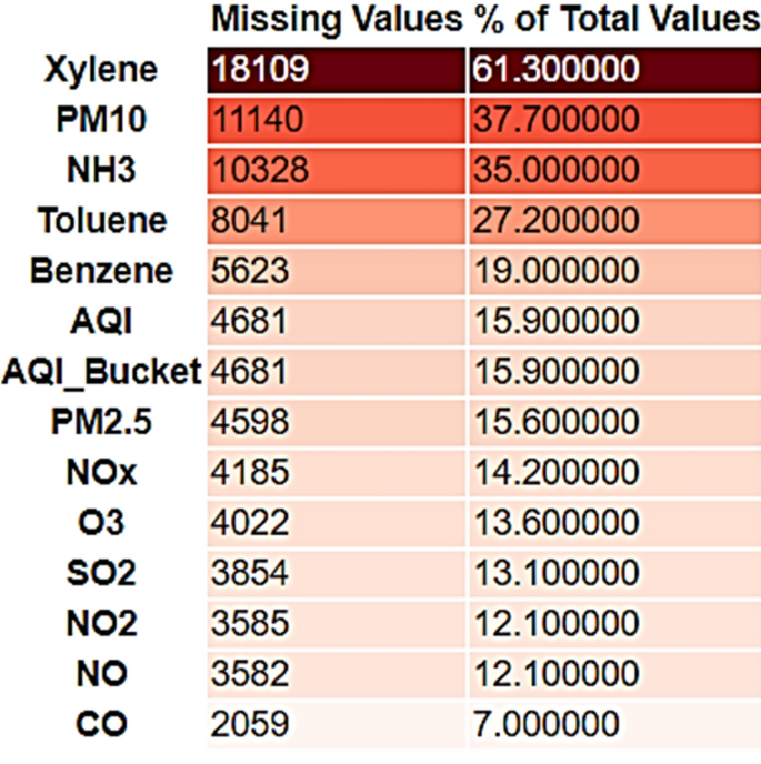
Quality of data is the first and most important prerequisite for effective visualization and creation of efficient ML models. The preprocessing steps help in reducing the noise present in the data which eventually increases the processing speed and generalization capability of ML algorithms. Outliers and missing data are the two most common errors in data extraction and monitoring applications. The data preprocessing step performs various operations on data such as filling out not-a-number (NAN) data, removing or changing outlier data, etc. Figure 2 shown below presents a view of the missing values in each feature of the dataset. Observe that among all other features, Xylene has the most missing values and CO has the least missing values. A large number of missing values may be existing due to a variety of factors, such as a station that can sense data but does not possess a device to record it.
All the missing values are filled with the median values against each feature to solve the missing data problem. Next, a normalisation process has been applied to standardize the data, ensuring that the significance of variables is unaffected by their ranges or units. The data normalisation process helps to bring different data attributes into a similar scale of measurement. This process plays a vital role in the stable training of ML models and boosts performance. The datatypes of all the variables are also examined during normalisation. For example, the dataset is collected from different monitoring stations which deal with different representations of dates. Thus, the date ‘Monday, May 17, 2021’ may be represented as ‘17/5/2021’ or as ‘17–05-2021’ etc. Such date feature has been normalised through the datetime Python library.
Feature selection
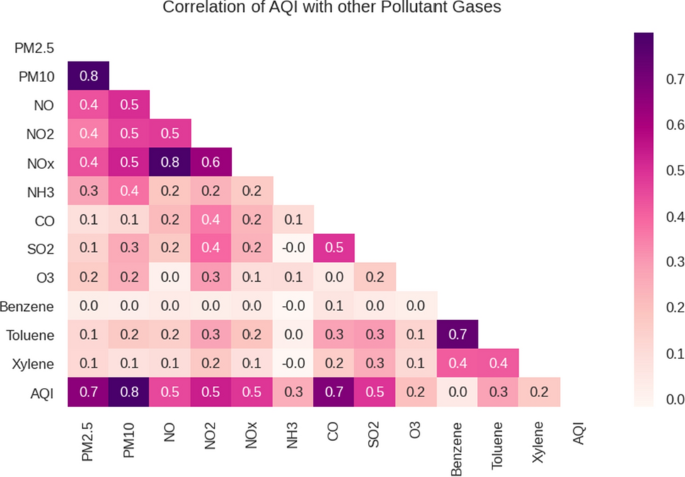
The CPCB dataset under study involves a specific parameter viz, AQI and government agencies use this parameter to alert people about the quality of the air and also practice forecasting it. According to the National Ambient Air Quality Standards, there are six AQI categories: good (0–50), satisfactory (51–100), moderate (101–200), poor (201–300), very poor (301–400), and severe (401–500). Scholars in the realm suggest that reducing input variables lowers the computational cost of modeling and enhances prediction performance. A correlation-based feature selection method has been exploited in the present work to determine the optimal number of input variables (pollutants) when developing a predictive model. Statistical correlation-based feature selection algorithms compute correlations between every pair of the input variable and the target variable. The variables possessing the strongest correlation with the target variable are then filtered for further study. Since many ML algorithms are sensitive to outliers, any feature in the input dataset which does not follow the general trend of that data must be found. For the present dataset, a correlation-based statistical outliers detection method has been applied to identify the outliers. To select significant features, the correlation analysis of the AQI feature has been exercised with features of other pollutants. Figure 3, shown below clearly reveals that pollutants PM10, PM2.5, CO, NO2, SO2, NOX, and NO are generally responsible for the AQI to attain higher values. These pollutants are correlated with AQI based on the correlation values above the threshold of 0.4.
Table 3 given below shows the exact correlation values of each pollutant of the dataset with AQI.
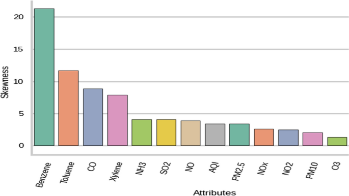
Many ML models function better when data have a normal distribution and underperform when data have a skewed distribution. Therefore, it is necessary to identify the skewness being present in the features and to perform some transformations and mappings which convert the skewed distribution into a normal distribution. Figure 4, given below shows that the features of Benzene, Toluene, CO, and Xylene are highly skewed. To make these skewed features more normal, the logarithmic transformations have been used to reduce the impact of outliers by normalising magnitude differences.
Exploratory data analysis
This section of the present study deals with data exploration and analysis for finding various hidden patterns present in the dataset. Exploratory data analysis is the first step in data analytics which is performed before applying any ML model. Under this, the following important things are being analyzed: (a) exploring statuses and trends of air pollutants over the past six years i.e. from 2015 to 2020; (b) exploring the distribution of pollutants in the air along with top-six polluted cities with their average AQI values; and (c) estimating top four pollutants which are directly involved in increasing the AQI values.
Exploring the trends of air pollutants over the last six years
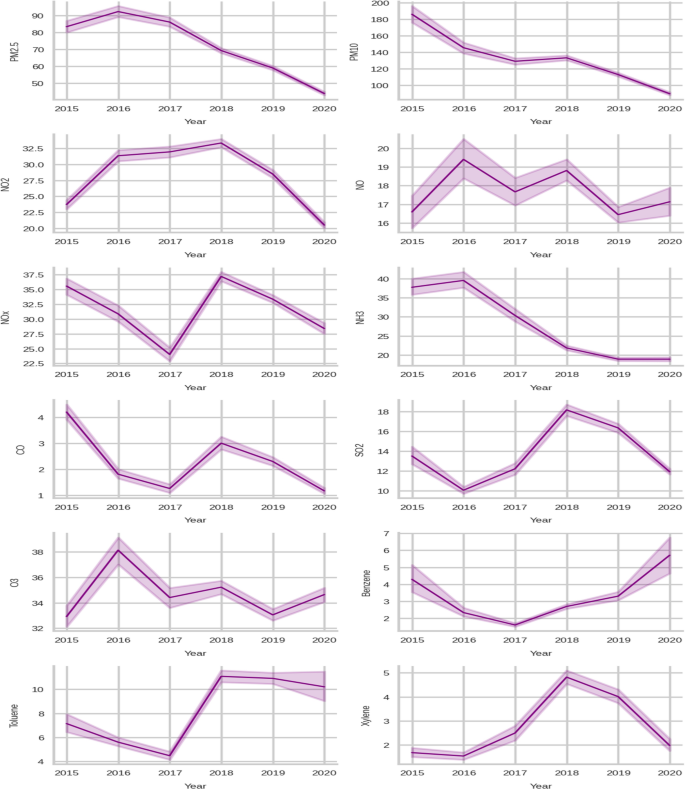
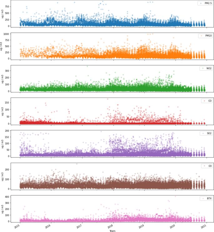
India has become one of the few countries having the most severe air pollution resulting from rapid industrialization and booming urbanization over the last several years. Air pollution is among grave public health and environmental issues, and the Health Effects Institute (HEI) ranks it among the top five global risk factors for mortality (IHME 2019). According to the HEI research, the emission of PM was the third leading cause of death in 2017, and this rate was highest in India. Based on the emissions of PM2.5 and other pollutants, the World Health Organization (WHO) ranked India as the fifth most polluted country (Gurjar, 2021). The trends of various pollutants from 2015 to 2020 are observed and shown in the figure below (Fig. 5). Observe that except for O3 and Benzene, all other pollutants exhibited a significant fall in 2020. The year 2020 witnessed the most strict lockdown in the history of mankind and ceased industrial, automobile, and aviation activities in India and the world served as some ambrosia for the ailing environment and air.
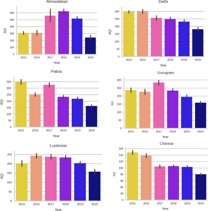
Figure 6 shown below depicts the average AQI values over the aforementioned tenure for the six most polluted cities in India.
Pollutants that are directly involved in increasing AQI values
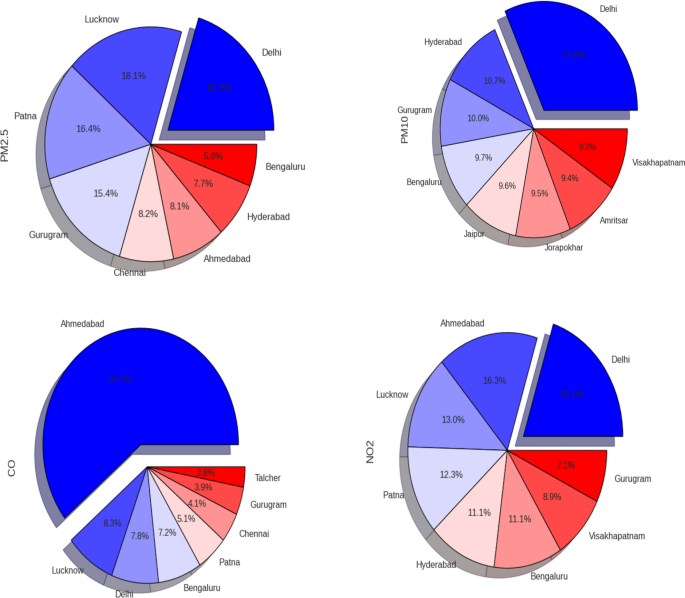
The correlation values between different pollutants and AQI have been exercised and the pollutants for which this correlation value is greater than the threshold of 0.5, i.e. the correlation is strongly positive have been identified. Figure 7 shown below depicts the concentration of four such pollutants in various cities in India.
Results and discussion
This section deals with the experimental design and empirical analysis for predicting AQI values through the pollutants present in the air. The air pollution dataset is split into training (75%) and testing (25%) subsets before evaluating ML models. The Google Colab Pro cloud platform with Intel(R) Xeon(R) CPU @ 2.30 GHz, Tesla P100-PCIE-16 GB, 12.8 GB RAM, and 180 GB of disc space has been utilized for executing Python scripts. The Python libraries like Scikit-learn, NumPy, Pandas, Seaborn, etc. are exploited for various data processing tasks. Next, the dataset is explored with the motive to find the overall value of the AQI with respect to those pollutants which have a significant role in raising the AQI value. In Fig. 8 shown below, a timeline graph of AQI is depicted over some particular pollutants which are directly responsible for higher values of AQI. From Fig. 8, it is clear that each pollutant grows and drops year after year, and their values do not remain constant every year. PM2.5 and PM10 have seasonal effects, with higher pollution levels in the winter than in the summer. After 2018, the level of SO2 began to rise, but the level of O3 stayed unchanged from 2018 to 2020. The same trend can be seen in BTXFootnote 2 levels as well. Except for CO, practically every pollutant has exhibited seasonal variations.
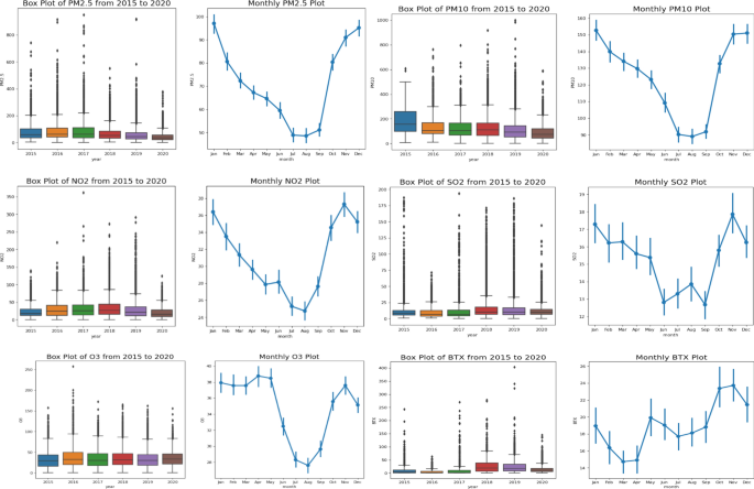
To examine the seasonality of the data thoroughly, Box plot visualizations are employed. Box plots categorise data into different periods by grouping the entire information in years and months. Figure 9 presents the Box plots of various pollutants over time, both annually and monthly. Notice that pollution levels in India decrease between June and August. It may be the consequence of the inception of the Monsoon in the Indian subcontinent during this tenure. BTX levels exhibit a significant drop between March and April, a modest rise from May to September, and a sharp surge from October to December. The median values for 2020 are lower than those for previous years, indicating that pollution may have decreased substantially in 2020. Strict lockdown ceased human and industrial activities in India during the COVID-19 pandemic are the obvious reasons for this observed phenomenon.
Next, the detailed development of ML-based AQI prediction models is discussed. Finally, the performance of the AQI forecasting models is evaluated. The target attribute, AQI_Bucket has some missing values which result in the unequal splitting of the classes. Many ML models ignore this imbalanced datasets problem which may lead to poor classification and prediction performances. To overcome this data imbalance problem, the SMOTE (Synthetic Minority Oversampling Technique) has been applied. In this technique, the algorithm synthesizes new elements for minority classes rather than creating copies of already existing elements. It functions by randomly choosing a point from the minority class and computing the k-nearest neighbor distances for the selected point. The newly created synthetic points are added between the chosen point and its neighbors. To implement SMOTE for class imbalance, we have used an imbalanced-learn Python library in the SMOTE class. Now, five popular ML models, KNN, Gaussian Naive Bayes (GNB), SVM, RF, and XGBoost have been employed to predict the AQI level with SMOTE and without SMOTE resampling technique. Table 4 shown below presents the results of used ML models in terms of accuracy, precision, recall, and F1-score during the training phase. Precision tells the fraction of relevant instances present in the retrieved instances, while recall is the fraction of relevant instances that have been retrieved. Accuracy is the ratio of the correctly labeled attributes to the whole pool of variables. F1-score is a weighted average of precision and recall. Note that the XGBoost model achieved the highest accuracy, while the SVM model exhibited the lowest accuracy.
The performances of the ML models for the training set are evaluated against the standard performance parameters, viz MAE, RMSE, Root Mean Squared Logarithmic Error (RMSLE), and coefficient of determination, i.e. R2 (Table 5). These performance measures have been exploited extensively in the literature. Table 5 given below provides error statistics of the ML models applied with and without SMOTE resampling technique on the training set. The XGBoost model outperformed other models in terms of error statistics when exercised without the SMOTE technique. On the other hand, the RF model performed relatively good among others in terms of error statistics when exercised with the SMOTE technique. The XGBoost model performed equally good in this area in terms of MAE and RMSLE. These observations are marked bold in Table 5.
Table 6 shown below presents the results of employed ML models obtained during the testing phase. It is evident from Table 6 that the XGBoost model surpassed the other models again, whereas the SVM model attained the lowest accuracy in the testing phase too.
The performances of the ML models for the testing set are evaluated against the standard performance parameters as above (Table 7).
The above table summarizes the performances of various ML models applied with and without SMOTE resampling technique on the testing set. It is observed that all ML models exhibited improvement in almost all assessment metrics when applied with SMOTE resampling technique. The GNB model attained the best values of R2 in both cases. The XGBoost model performed the best in terms of error statistics and attained the most optimum values in both experimental genres. These observations are marked bold in Table 7.
Conclusion
Prediction of air quality is a challenging task because of the dynamic environment, unpredictability, and variability in space and time of pollutants. The grave consequences of air pollution on humans, animals, plants, monuments, climate, and environment call for consistent air quality monitoring and analysis, especially in developing countries. However, lesser attention for researchers has been observed for AQI prediction for India. In the present work, air pollution data of 23 Indian cities for a tenure of six years are investigated. The dataset is cleaned and preprocessed first by filling NAN values, addressing outliers, and normalising data values. Then correlation-based feature selection technique is exercised to filter AQI affecting pollutants for further study and logarithmic transformations are applied to the skewed features. The exploratory data analysis methods are exercised to find various hidden patterns present in the dataset. It was found that almost all pollutants exhibited a significant fall in 2020. The data imbalance problem is addressed by the SMOTE analysis. The dataset is split into train-test subsets by the ratio of 75–25% respectively. ML-based AQI prediction is carried out with and without SMOTE resampling technique and a comparative analysis is presented. The results of ML models for both the train-test subsets are presented in terms of standard metrics like accuracy, precision, recall, and F1-Score. For both the train-test sets, the XGBoost model attained the highest accuracy and the SVM model exhibited the lowest accuracy. The classical statistical error metrics, namely MAE, RMSE, RMSLE, and R2 are then evaluated to assess and compare the performances of ML models. The XGBoost model comes out to be the overall best performer by attaining the optimum values in both training and testing phases. For the training phase, the RF model performed relatively good when exercised with SMOTE. On the other hand, almost all ML models exhibited improvements in the testing phase. In this phase, the GNB model attained the best results for R2 in target predictions. The present research endeavors to contribute to the literature by addressing air quality analysis and prediction for India which might have not been properly studied. This work can be extended by employing deep learning techniques for AQI prediction.
Notes
The dataset can be downloaded from: https://app.cpcbccr.com/ccr/#/caaqm-dashboard-all/caaqm-landing/data.
BTX is the combined name given to Benzene, Toluene, and Xylene.
References
Alade IO, Rahman MAA, Saleh TA (2019a) Predicting the specific heat capacity of alumina/ethylene glycol nanofluids using support vector regression model optimized with Bayesian algorithm. Sol Energy 183:74–82. https://doi.org/10.1016/j.solener.2019.02.060
Alade IO, Rahman MAA, Saleh TA (2019b) Modeling and prediction of the specific heat capacity of Al2 O3/water nanofluids using hybrid genetic algorithm/support vector regression model. Nano-Struct Nano-Objects 17:103–111. https://doi.org/10.1016/j.nanoso.2018.12.001
Al-Jamimi HA, Saleh TA (2019) Transparent predictive modelling of catalytic hydrodesulfurization using an interval type-2 fuzzy logic. J Clean Prod 231:1079–1088. https://doi.org/10.1016/j.jclepro.2019.05.224
Al-Jamimi HA, Al-Azani S, Saleh TA (2018) Supervised machine learning techniques in the desulfurization of oil products for environmental protection: a review. Process Saf Environ Prot 120:57–71. https://doi.org/10.1016/j.psep.2018.08.021
Al-Jamimi HA, Bagudu A, Saleh TA (2019) An intelligent approach for the modeling and experimental optimization of molecular hydrodesulfurization over AlMoCoBi catalyst. J Mol Liq 278:376–384. https://doi.org/10.1016/j.molliq.2018.12.144
Ayturan YA, Ayturan ZC, Altun HO, Kongoli C, Tuncez FD, Dursun S, Ozturk A (2020) Short-term prediction of PM2.5 pollution with deep learning methods. Global NEST J 22(1):126–131
Bellinger C, Jabbar MSM, Zaïane O, Osornio-Vargas A (2017) A systematic review of data mining and machine learning for air pollution epidemiology. BMC Public Health. https://doi.org/10.1186/s12889-017-4914-3
Bhalgat P, Bhoite S, Pitare S (2019) Air Quality Prediction using Machine Learning Algorithms. Int J Comput Appl Technol Res 8(9):367–370. https://doi.org/10.7753/IJCATR0809.1006
Castelli M, Clemente FM, Popoviˇc A, Silva S, Vanneschi L (2020) A machine learning approach to predict air quality in California. Complexity 2020(8049504):1–23. https://doi.org/10.1155/2020/8049504
Dalberg (2019) Air pollution and its impact on business: the silent pandemic. https://www.cleanairfund.org/wp-content/uploads/2021/04/01042021_Business-Cost-of-Air-Pollution_Long-Form-Report.pdf
Deshpande T (2021) India Has 9 Of World's 10 most-polluted cities, but few air quality monitors. indiaspend. https://www.indiaspend.com/pollution/india-has-9-of-worlds-10-most-polluted-cities-but-few-air-quality-monitors-792521
Doreswamy HKS, Yogesh KM, Gad I (2020) Forecasting Air pollution particulate matter (PM2.5) using machine learning regression models. Procedia Comput Sci 171:2057–2066. https://doi.org/10.1016/j.procs.2020.04.221
Fahad S, Sönmez O, Saud S, Wang D, Wu C, Adnan M, Turan, V (2021a) Plant growth regulators for climate-smart agriculture (1st ed.). CRC Press. https://doi.org/10.1201/9781003109013
Fahad, S, Sönmez O, Saud S, Wang D, Wu C, Adnan M, Turan V (2021b) Sustainable soil and land management and climate change (1st ed.). CRC Press. https://doi.org/10.1201/9781003108894
Gopalakrishnan V (2021) Hyperlocal air quality prediction using machine learning. Towards data science. https://towardsdatascience.com/hyperlocal-air-quality-prediction-using-machine-learning-ed3a661b9a71
Gurjar BR (2021) Air pollution in india: major issues and challenges. energy future 9(2):12–27. https://www.magzter.com/stories/Education/Energy-Future/AIR-POLLUTION-IN-INDIA-MAJOR-ISSUES-AND-CHALLENGES
IHME (2019) State of global air 2019 report. http://www.healthdata.org/news-release/state-global-air-2019-report
Liang Y, Maimury Y, Chen AH, Josue RCJ (2020) Machine learning-based prediction of air quality. Appl Sci 10(9151):1–17. https://doi.org/10.3390/app10249151
Madan T, Sagar S, Virmani D (2020) Air quality prediction using machine learning algorithms–a review. In: 2nd international conference on advances in computing, communication control and networking (ICACCCN) pp 140–145. https://doi.org/10.1109/ICACCCN51052.2020.9362912
Madhuri VM, Samyama GGH, Kamalapurkar S (2020) Air pollution prediction using machine learning supervised learning approach. Int J Sci Technol Res 9(4):118–123
Mahalingam U, Elangovan K, Dobhal H, Valliappa C, Shrestha S, Kedam G (2019) A machine learning model for air quality prediction for smart cities. In: 2019 international conference on wireless communications signal processing and networking (WiSPNET). IEEE 452–457. https://doi.org/10.1109/WiSPNET45539.2019.9032734
Monisri PR, Vikas RK, Rohit NK, Varma MC, Chaithanya BN (2020) Prediction and analysis of air quality using machine learning. Int J Adv Sci Technol 29(5):6934–6943
Nahar K, Ottom MA, Alshibli F, Shquier MA (2020) Air quality index using machine learning—a jordan case study. COMPUSOFT, Int J Adv Comput Technol 9(9):3831–3840
Patil RM, Dinde HT, Powar SK (2020) A literature review on prediction of air quality index and forecasting ambient air pollutants using machine learning algorithms 5(8):1148–1152
Rogers CD (2019) Pollution's impact on historical monuments pollution's impact on historical monuments. SCIENCING. https://sciencing.com/about-6372037-pollution-s-impact-historical-monuments.html
Rybarczyk Y, Zalakeviciute R (2017) Regression models to predict air pollution from affordable data collections. In: H. Farhadi (Ed.), Machine learning advanced techniques and emerging applications pp 15–48. IntechOpen. https://doi.org/10.5772/intechopen.71848
Rybarczyk Y, Zalakeviciute R (2021) Assessing the COVID-19 impact on air quality: a machine learning approach. Geophys Res Lett. https://doi.org/10.1029/2020GL091202
Sanjeev D (2021) Implementation of machine learning algorithms for analysis and prediction of air quality. Int. J. Eng. Res. Technol. 10(3):533–538
Sönmez O, Saud S, Wang D, Wu C, Adnan M, Turan V (2021) Climate change and plants: biodiversity, growth and interactions (S. Fahad, Ed.) (1st ed.). CRC Press. https://doi.org/10.1201/9781003108931
Soundari AG, Jeslin JG, Akshaya AC (2019) Indian air quality prediction and analysis using machine learning. Int J Appl Eng Res 14(11):181–186
Sweileh WM, Al-Jabi SW, Zyoud SH, Sawalha AF (2018) Outdoor air pollution and respiratory health: a bibliometric analysis of publications in peer-reviewed journals (1900–2017). Multidiscip Respiratory Med. https://doi.org/10.1186/s40248-018-0128-5
Zhu D, Cai C, Yang T, Zhou X (2018) A machine learning approach for air quality prediction: model regularization and optimization. Big Data and Cognitive Comput. https://doi.org/10.3390/bdcc2010005
Acknowledgements
No organization funded the present research.
Author information
Authors and Affiliations
Corresponding author
Ethics declarations
Conflict of interest
The authors declare that they have no conflict of interest.
Additional information
Editorial responsibility: M. Abbaspour.
Rights and permissions
About this article
Cite this article
Kumar, K., Pande, B.P. Air pollution prediction with machine learning: a case study of Indian cities. Int. J. Environ. Sci. Technol. 20, 5333–5348 (2023). https://doi.org/10.1007/s13762-022-04241-5
Received:
Revised:
Accepted:
Published:
Issue Date:
DOI: https://doi.org/10.1007/s13762-022-04241-5


