Algebraic aspects of hypergeometric differential equations

Abstract

We review some classical and modern aspects of hypergeometric differential equations, including A-hypergeometric systems of Gel$'$fand, Graev, Kapranov and Zelevinsky. Some recent advances in this theory, such as Euler–Koszul homology, rank jump phenomena, irregularity questions and Hodge theoretic aspects are discussed with more details. We also give some applications of the theory of hypergeometric systems to toric mirror symmetry.

1 Introduction

Notational conventions

We use Italic letters M for rings, variables and modules; calligraphic letters ${\mathscr {D}}$ for sheaves; Roman letters ${{\,\mathrm{FL}\,}}$ for functors; Gothic letters for prime ideals ${\mathfrak {p}}$ and points ${\mathfrak {x}}$ of spaces.

Lattice elements $\mathbf{a }$ are in Roman bold; coordinate sets ${\varvec{t}}$ and other sets of functions or operators ${\varvec{\partial }}$ in Italic bold. $\Diamond$

1.1 Hypergeometric functions

The study of hypergeometric functions started more than two centuries ago and formed a important part of the work of Euler and Gauß. A power series

$$\begin{aligned} f(z)=\sum _{i=0}^{\infty } a_i z^i/i! \end{aligned}$$

is hypergeometric if the quotient $a_{i+1}/a_i$ of consecutive coefficients is a rational function in i. Traditional convention dictates that the exponential function is regarded as the standard hypergeometric function (to $a_{i+1}/a_i$ constant); this “explains” the choice of $a_i/i!$ over $a_i$ as series coefficient. Further examples include Bessel, Airy, trigonometric and (higher) logarithmic as well as all other special functions, and the hypergeometric functions that express roots of algebraic equations (Sturmfels 1996).

The continuing interest in hypergeometric functions stems to some extent from the fact that they are often solutions to very appealing linear differential equations taken from physics. For example, the Bessel functions $J_{\pm r}(x)$ of the first kind arise as solutions to a linear second order equation that shows up in heat and electromagnetic propagation in a cylinder, vibrations of circular membranes, and more generally when solving the Helmholtz or Laplace equation. Indeed, such connections to physics through differential equations prompted the first studies of (specific) hypergeometric functions. However, hypergeometric functions also appear in many other parts of mathematics: as we will see soon, each time an action of an algebraic torus on a space is observed, one can expect to find some differential equation of hypergeometric type connected to this situation. The abundance of toric varieties in geometry explains why there are so many different interesting hypergeometric functions. We discuss in Sect. 5 below one prominent case where hypergeometric differential equations prove to be useful: the so-called mirror symmetry phenomenon for certain smooth toric varieties. Other recent applications that are beyond the scope of this article include the holonomic gradient method in algebraic statistics (Hibi et al. 2017) or Feynman integral computations in quantum field theory (Nasrollahpoursamami 2016; Klausen 2019; de la Cruz 2019; Feng et al. 2020).

As it turns out, it is exactly the type of differential equation satisfied by a function that determines whether the function should be considered as hypergeometric, since these force the right kind of recursions on the series. The most successful approach to generalize hypergeometric differential equations to several variables was initiated by Gel$'$fand, Graev, Kapranov and Zelevinsky in the 1980s, and some of the features of this theory form the topic of this article. We start with some motivating examples.

Example 1.1

(The error function, part I) The (Gauß) error function ${{\,\mathrm{erf}\,}}(x)$ is defined by

$$\begin{aligned} {{\,\mathrm{erf}\,}}(z)=\frac{2}{\sqrt{\pi }}\int _0^z\exp (-t^2)\,\mathrm{d}t. \end{aligned}$$

While this integral cannot be solved in closed form, it can be developed into a convergent Taylor series

$$\begin{aligned} {{\,\mathrm{erf}\,}}(z)=\frac{2}{\sqrt{\pi }}z\sum _{i=0}^{\infty } a_i\frac{(-z^2)^i}{i!} \end{aligned}$$

(1)

where $a_i=1/(2i+1)$, so that

$$\begin{aligned} {{\,\mathrm{erf}\,}}(z)=\frac{2z}{\sqrt{\pi }}\left( 1-\frac{z^2}{3}+\frac{(z^2)^2}{10}-\frac{(z^2)^3}{42} -\frac{(z^2)^4}{216}+ \frac{(z^2)^5}{1320}\mp \cdots \right) \end{aligned}$$

is hypergeometric. $\Diamond$

The univariate hypergeometric functions are classified by the rational function $a_{i+1}/a_i$. More precisely, suppose that $a_{i+1}/a_i=P(i)/Q(i)$ where $P,Q\in {\mathbb {C}}[i]$ are monic with $P=\prod _{j=1}^p(i+\alpha _j)$ and $Q=\prod _{j=1}^q(i+\beta _j)$. Then the univariate hypergeometric function associated to P, Q is

$$\begin{aligned} _pF_q(\alpha _1,\ldots ,\alpha _p;\beta _1,\ldots ,\beta _q;z) =\sum _{i=0}^{\infty } \frac{a_i z^i}{i!} \end{aligned}$$

(2)

where $a_0=1$ and

$$\begin{aligned} \frac{a_{i+1}}{a_i}=\frac{(i+\alpha _1)(i+\alpha _2)\ldots (i+\alpha _p)}{(i+\beta _1) (i+\beta _2)\ldots (i+\beta _q)}. \end{aligned}$$

Example 1.2

(The error function, part II) It follows from (1) that ${{\,\mathrm{erf}\,}}(z)$ is, up to the factor $2z/\sqrt{\pi }$, equal to ${}_1F_1(1/2;3/2;-z^2)$, where

$$\begin{aligned} {}_1F_1(1/2;3/2;z)=1+\frac{z}{3}+\frac{z^2}{10}+\frac{z^3}{42} +\frac{z^4}{216}+ \frac{z^5}{1320}+\cdots \end{aligned}$$

is the Kummer confluent function which encodes all intrinsic analytic and combinatorial properties of ${{\,\mathrm{erf}\,}}(x)$ and, with $\theta _z=z\frac{d}{dz}$, satisfies the differential equation

$$\begin{aligned} \theta _z(\theta _z+1/2)\bullet (f)-z(\theta _z-1/2)\bullet (f)=0. \end{aligned}$$

(3)

The particular shape of this equation will be used in the next section for a conversion process from univariate hypergeometric functions to A-hypergeometric ones. $\Diamond$

In the following example we document how hypergeometric functions arise naturally from differential forms with parameters. The computation was apparently already known to Kummer; compare (Brieskorn and Knörrer 1986) for details. In modern terms, it represents the birth of the notion of a variation of Hodge structures.

Example 1.3

(Hypergeometry and Hodge filtrations) The equation $f_z=0$ with

$$\begin{aligned} f_z(u,v)=v^2-u(u-1)(u-z) \end{aligned}$$

defines for each $z\in {\mathbb {C}}\smallsetminus \{0,1\}$ a smooth curve $E_z$ over ${\mathbb {C}}$. Its projective closure $\overline{E}_z\subseteq {\mathbb {P}}^2_{{\mathbb {C}}}$ meets the line at infinity in a single point and is smooth as long as $z\not \in \{ 0,1,\infty \}$. The natural projection from $E_z$ to ${\mathbb {C}}$ via “forgetting v” is generically 2 : 1 and branches at 0, 1, z; the induced map $\overline{E}_z\longrightarrow {\mathbb {P}}^1_{{\mathbb {C}}}$ also branches at infinity.

The differential 1-form $\omega _z:=\mathrm{d}u/v$ is everywhere holomorphic and nowhere zero on $\overline{E}_z$; the existence of this “form of the first kind” in Riemann’s language makes the elliptic curve $\overline{E}_z$ a Calabi–Yau manifold in modern terms. The “form of the second kind” $\omega '_z:=\omega _z/(u-z)$ has a unique pole, at $u=z$, at which it is residue-free. Considering $v=v(u,z)$ as dependent variable and writing $\omega _z, \omega '_z$ in terms of u and z, one notes that $\frac{\partial }{\partial z}(\omega _z)=\frac{1}{2}\omega '_z$, and (compare especially (Brieskorn and Knörrer 1986, Page 685))

$$\begin{aligned} \frac{\partial }{\partial z}(\omega '_z)=\frac{3\mathrm{d}u}{4v(u-z)^2} =\underbrace{\frac{1}{4z(1-z)}}_{p(z)}\omega _z +\underbrace{\frac{-1+2z}{z(1-z)}}_{q(z)}\omega '_z +\mathrm{d}\left( \frac{v}{2(u-z)^2z(1-z)}\right) , \end{aligned}$$

the differential on the right being taken in u, v with z constant (and noting that on E one has $\mathrm{d}(u(u-1)(u-z))=2v\,\mathrm{d}v$).

Let $\lambda \in H_1(\overline{E}_z;{\mathbb {Z}})\simeq {\mathbb {Z}}\oplus {\mathbb {Z}}$ and set $I_1(\lambda )=\int _{\lambda }\omega _z$ and $I_2(\lambda ) =\int _{\lambda }\omega '_z$, multi-valued functions on $\overline{E}_z$ defined via elliptic integrals. The differential equations for $\omega _z,\omega '_z$ imply (compare (Brieskorn and Knörrer 1986, Lemma 12)) that $I_1(\lambda )$ and $I_2(\lambda )$ are solutions to

$$\begin{aligned} f''-qf'=pf, \end{aligned}$$

(4)

with singularities at 0, 1 and $\infty$. It is the special case $1=2a=2b=c$ of the general Gauß hypergeometric differential equation

$$\begin{aligned} f''+\frac{c-(a+b+1)t}{z(1-z)}f'=\frac{ab}{z(1-z)}f \end{aligned}$$

with solution space basis given by Gauß’ hypergeometric functions

$$\begin{aligned} F_1= & {} \sum _{n=0}^{\infty } \frac{[a]_n[b]_n}{[c]_n}\frac{z^n}{n!},\\ F_2= & {} -\sqrt{-1}\sum _{n=0}^{\infty } \frac{[a]_n[b]_n}{[c]_n}\frac{(1-z)^n}{n!}, \end{aligned}$$

which have singularities at $0,\infty$ and $1,\infty$ respectively.

Suppose $\lambda _z,\lambda '_z$ are the standard basis (the minimal geodesics) for the first homology group of the torus $\overline{E}_z$. Then two elementary (but non-trivial) computations reveal:

• (1) analytic continuation of the solution space basis $F=(F_1,F_2)^T$ around the points $z=0$ and $z=1$ corresponds to multiplication of F by $M_0=\begin{pmatrix} 1&{}0 \\ -2&{}1 \end{pmatrix}$ and $M_1=\begin{pmatrix} 1&{} 2 \\ 0&{}1 \end{pmatrix}$ respectively;

• (2) the map

  

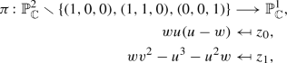
  is a bundle with fiber $\overline{E}_{z_1/z_0}$ that admits an Ehresmann connection. In particular, the cohomology classes of the fibers allow parallel transport. The induced vector bundle with fiber $H_1(\overline{E}_z;{\mathbb {Z}})={\mathbb {Z}}\lambda _z+{\mathbb {Z}}\lambda '_z$ admits a monodromy action, lifting the loops around $z=(0,1)$ and $z=(1,1)$. Analysis of the geometry of $\pi$ shows that this monodromy is given again by the actions of $M_1$ and $M_2$ respectively.

More abstractly, the D-module on the base of $\pi$ corresponding to the (derived) direct image (compare Notation 4.1) of the structure sheaf on the source of $\pi$, also known as the Gauß –Manin system, has monodromy action via $M_1,M_2$.

On the complement of the points $0, 1, \infty$ this $D_z$-module is a vector bundle with a flat connection. The fibers of this vector bundle are the cohomology groups $H^1(\overline{E}_{z_1 /z_0};{\mathbb {C}})$. This vector bundle is actually a variation of pure Hodge structures of weight 1 where the (1, 0)-part is generated by the differential form $\omega _z$, the variation of this (1, 0)-subbundle being described by (4).

It follows that, up to scalars, $I_1(\lambda _z)=F_1(z)$, $I_2(\lambda _z)=F_2(z)$. In particular, the ratio $\tau (z)=I_1(\lambda _z)/I_2(\lambda _z)$ is the modulus of the elliptic curve in the sense that the fiber over z is isomorphic to the quotient of ${\mathbb {C}}$ by ${\mathbb {Z}}+\sqrt{-1}\tau \cdot {\mathbb {Z}}$.

We will take up the discussion of Hodge structures associated to more general univariate hypergeometric operators (see Eq. (7) below) later in Sect. 4 (see page 33). $\Diamond$

1.2 From univariate to GKZ and back

In the 1980s, the Russian school around I.M. Gel$'$fand found a universal way of encoding univariate hypergeometric functions by way of certain systems of PDEs that arise from an integer matrix A and complex parameter vector $\beta$. We start with the general definition and then explain how univariate hypergeometric functions arise as solutions of these D-modules.

Notation 1.4

In the first three sections of this article,

$$\begin{aligned} A=(\mathbf{a }_1,\ldots ,\mathbf{a }_n)\in {\mathbb {Z}}^{d\times n} \end{aligned}$$

denotes an integer matrix with d rows and n columns. In the last two sections, A will still be integer, but at least sometimes of size $(d+1)\times (n+1)$. $\Diamond$

For convenience, we place the following constraints on the matrix A; they make concise statements possible, or at least easier to make.

Convention 1.5

(Standard assumptions on A) With A as above, A spans a semigroup

$$\begin{aligned} {\mathbb {N}}A:=\sum _{j=1}^n {\mathbb {N}}\mathbf{a }_j \subseteq {\mathbb {Z}}A \end{aligned}$$

inside ${\mathbb {Z}}^d$. Throughout we assume that

• the group ${\mathbb {Z}}A$ generated by A agrees with ${\mathbb {Z}}^d$ (A is full);

• the semigroup ${\mathbb {N}}A$ contains no units besides $\mathbf{0 }$ (A is pointed). We note that pointedness of A is equivalent to the existence of a group homomorphism from ${\mathbb {Z}}^d$ to ${\mathbb {Z}}$ that is positive on every $\mathbf{a }_j$.

$\Diamond$

We now give the definition of the main character of our story.

Definition 1.6

(A-hypergeometric system, Gel’fand et al. (1987)) Fix $A\in {\mathbb {Z}}^{d\times n}$ as in Convention 1.5 and choose $\beta \in {\mathbb {C}}^d$. Let

$$\begin{aligned} D_A:={\mathbb {C}}[{\varvec{x}}]{\langle {{\varvec{\partial }}}\rangle } \end{aligned}$$

be the n-th Weyl algebra over ${\mathbb {C}}$. Here ${\varvec{x}}=x_1,\ldots ,x_n, {\varvec{\partial }}=\partial _1,\ldots ,\partial _n$, and $\partial _j$ is identified with the partial differentiation operator $\frac{\partial }{\partial x_j}$. We also let

$$\begin{aligned} R_A:={\mathbb {C}}[{\varvec{\partial }}]\subseteq D_A \end{aligned}$$

denote the polynomial subring.

Letting $\theta _j$ stand for $x_j\partial _j$, the Euler operator $E_i$ is

$$\begin{aligned} E_i=\sum _{j=1}^n a_{i,j}\theta _j. \end{aligned}$$

For each $\mathbf{u }\in {\mathbb {Z}}^n$ in the kernel of A its box operator is

$$\begin{aligned} \Box _{\mathbf{u }}={\varvec{\partial }}^{\mathbf{u }_+}-{\varvec{\partial }}^{\mathbf{u }_-}, \end{aligned}$$

where $(\mathbf{u }_+)_j=\max \{0,\mathbf{u }_j\}$ and $(\mathbf{u }_-)_j=\max \{0,-\mathbf{u }_j\}$. The toric ideal $I_A$ is the $R_A$-ideal generated by all $\Box _{\mathbf{u }}$ with $\mathbf{u }\in \ker A$. Finally, the hypergeometric ideal and module to $A,\beta$ are

$$\begin{aligned} H_A(\beta ):=D_A(I_A,\{E_i-\beta _i\}_1^d),\qquad \qquad M_A(\beta ):=D_A/H_A(\beta ). \end{aligned}$$

$\Diamond$

Before we embark on a general discussion of these modules we wish to distinguish two special subclasses that will play a lead role.

Definition 1.7

The matrix A is homogeneous if the following equivalent properties are satisfied:

• there is a group homomorphism from ${\mathbb {Z}}^d$ to ${\mathbb {Z}}$ that sends every $\mathbf{a }_j$ to $1\in {\mathbb {Z}}$;

• the vector $(1,1,\ldots ,1)$ is in the row span of A;

• the ideal $I_A$ is standard graded and thus defines a projective variety inside projective $(n-1)$-space.

$\Diamond$

Definition 1.8

The semigroup ${\mathbb {N}}A$ is saturated if ${\mathbb {N}}A$ agrees with the intersection of ${\mathbb {Z}}A$ with the cone ${\mathbb {R}}_{\ge 0} A$ spanned by the columns of A viewed as elements of ${\mathbb {R}}^n={\mathbb {Z}}^n\otimes _{{\mathbb {Z}}} {\mathbb {R}}$. $\Diamond$

In a series of articles, including Gel’fand et al. (1987, 1989, 1990), the basic theory of these linear PDEs was developed by the Gel’fand school. The initial motivation came from Aomoto type integrals

$$\begin{aligned} Y(\beta ;{\varvec{x}})=\int _Ct^{\beta }\exp \left( \sum _{i=1}^nx_it^{\mathbf{a }_i}\right) \frac{\mathrm{d}t_1}{t_1}\cdots \frac{\mathrm{d}t_d}{t_d} \end{aligned}$$

(5)

depending on a complex parameter vector $\beta \in {\mathbb {C}}^d$, It is not hard to verify that a hypergeometric function defined by the integral (5) is annihilated by both the Euler operators and the box operators (Gel’fand et al. 1990; Adolphson 1994) but it took a decade to arrive at the general formulation given here.

It turns out that every univariate hypergeometric function arises as a solution of an A-hypergeometric system; we sketch next the steps to construct the proper $A,\beta$. The general hypergeometric univariate differential equation is

$$\begin{aligned} \prod _{v_j>0} \prod _{\ell =0}^{v_j-1} (v_j \theta _z +c_j -l) = z \cdot \prod _{v_j<0} \prod _{\ell =0}^{|v_j|-1} (v_j \theta _z +c_j -l). \end{aligned}$$

(6)

It is elementary, but not always trivial, to bring a differential equation derived from a series expansion of a hypergeometric function into this shape; it may require changes of variables in z. Note that ${}_pF_q(\alpha ;\beta ;z)$ is a solution to the special form

$$\begin{aligned} \theta _z\prod _{j=1}^q(\theta _z+\beta _j-1)=z\cdot \prod _{j=1}^p(\theta _z+\alpha _j) \end{aligned}$$

(7)

as one can see from applying the two operators to the power series (2).

Let $\mathbf{v }$ and $\mathbf{c }$ be the vectors with entries $v_j$ and $c_j$ respectively. For ${}_2F_1$ (equal to the function $F_1$ in Example 1.3), $\mathbf{v }=(1,1,-1,-1)$ while for the Kummer confluent function ${}_1F_1$, $\mathbf{v }=(1,1,-1)$.

Now, in order to manufacture A and $\beta$ from Eq. (6), choose an integral matrix A such that ${\mathbb {Z}}\cdot \mathbf{v }=\ker A$ and set $\beta =A\cdot \mathbf{c }$. Then the solutions of $H_A(\beta )$ (in other words, the functions annihilated by every operator in this left ideal) “contain the solutions to (6)” in the following sense.

Example 1.9

(The GKZ-system to the Kummer confluent function) Consider the system of partial differential equations

$$\begin{aligned} \left( 1\theta _1+1\theta _3\right) \bullet (u)= & {} (-1/2)u \end{aligned}$$

(8)

$$\begin{aligned} \left( 1\theta _2+1\theta _3\right) \bullet (u)= & {} (0)u \end{aligned}$$

(9)

$$\begin{aligned} \left( \partial _1\partial _2-\partial _3\right) \bullet (u)= & {} 0 \end{aligned}$$

(10)

in $x_1,x_2,x_3$. This is the A-hypergeometric system to

$$\begin{aligned} A=\begin{pmatrix} 1&{}\quad 0&{}\quad 1\\ 0&{}\quad 1&{}\quad 1 \end{pmatrix},\qquad \beta =\begin{pmatrix} -1/2\\ 0 \end{pmatrix}, \end{aligned}$$

(11)

since $v=(1,1,-1)$ is the ${\mathbb {Z}}$-kernel of A.

Equation (8) forces any solution u to be homogeneous (and of degree $-1/2$) under the grading that attaches the weights (1, 0, 1) to $(x_1,x_2,x_3)$. Similarly, Eq. (9) asserts that u is homogeneous of weight zero if $(x_1,x_2,x_3)\mapsto (0,1,1)$. It follows that one can write

$$\begin{aligned} u(x_1,x_2,x_3)=x_1^ax_2^bx_3^c\, g(x_1x_2/x_3) \end{aligned}$$

where the monomial $x_1^ax_2^bx_3^c$ is of bi-degree $(-1/2,0)$, and g is a univariate function.

Set $z=x_1x_2/x_3$ and write

$$\begin{aligned} g(z)=\sum _{i=0}^{\infty } g_iz^i. \end{aligned}$$

Enforcing the vanishing of $\partial _1\partial _2-\partial _3$ on $u(x_1,x_2,x_3)$ as suggested by Eq. (10) implies the recurrence relations

$$\begin{aligned} (c-i)g_i=(a+i+1)(b+i+1)g_{i+1} \end{aligned}$$

for all i, and the starting condition

$$\begin{aligned} \partial _1\partial _2\bullet (x_1^ax_2^b)=0. \end{aligned}$$

For $a=0$, observing that $x_1^ax_2^bx_3^c$ is of bi-degree $(-1/2,0)$, we infer $b=-c=1/2$ and thus the recurrence is

$$\begin{aligned} (-1/2-i)g_i=(i+1)(1/2+i+1)g_{i+1}, \end{aligned}$$

showing that g(z) essentially agrees with the Kummer confluent function. $\Diamond$

Example 1.10

(GKZ-system to ${}_2F_1$) Take Eq. (7) with $p=q=2$ and $\mathbf{c }=(1,c,a,b)$. Then $\mathbf{v }=(1,1,-1,-1)$ and the matrix A can be chosen as

$$\begin{aligned} A=\begin{pmatrix} 1&{}\quad 1&{}\quad 1&{}\quad 1\\ 1&{}\quad 0&{}\quad 0&{}\quad 1\\ 0&{}\quad 1&{}\quad 0&{}\quad 1 \end{pmatrix}, \end{aligned}$$

so that $\beta =A\cdot \mathbf{c }=(c-1,-a,-b)$. The three Euler operators $\{\sum _{j=1}^4 a_{i,j}\theta _j-\beta _i\}_{i=1}^3$ annihilate each solution, so every monomial $x^{\mathbf{u }}$ in the power series expansion of every solution to the A-hypergeometric system must satisfy the three conditions

$$\begin{aligned} \left( u_1+u_2+u_3+u_4\right)= & {} \beta _1;\\ \left( u_1+u_4\right)= & {} \beta _2;\\ \left( u_2+u_4\right)= & {} \beta _3. \end{aligned}$$

For a monomial $x^{\mathbf{u }}$, we call $A\cdot \mathbf{u }\in {\mathbb {Z}}A$ the A-degree of $x^{\mathbf{u }}$. Then, every solution $u(x_1,x_2,x_3,x_4)$ can be written as a univariate function g in $\frac{x_1x_4}{x_2x_3}$, multiplied by a monomial of A-degree $\beta$. As in the previous example, one can use the fact that $\Box _{\mathbf{v }}$ kills u to show that g satisfies the Gauß hypergeometric differential equation. $\Diamond$

Of course, the kernel of A being ${\mathbb {Z}}\cdot \mathbf{v }$ means that $A\in {\mathbb {Z}}^{(n-1)\times n}$ and $I_A=(\Box _{\mathbf{v }})$ is principal. On the other hand, the A-hypergeometric paradigm also encodes multivariate hypergeometric series of higher rank (namely $n-d$) when $d<n-1$. The solutions to $H_A(\beta )$ use n variables and satisfy d homogeneities, so that effectively they are functions in $n-d$ independent quantities. Some aspects of the translation between the two setups is discussed in Berkesch et al. (2019). The advantage of the A-hypergeometric point of view is that it allows hypergeometric functions to be studied with methods coming from algebraic geometry, commutative algebra, and the theory of torus actions. We describe in the following sections some of the advances and some of the new problems that have been created through these new techniques.

1.3 Solutions

While we do not focus very much on solutions of A-hypergeometric systems in this survey, it is only fair to indicate to some extent the development of the understanding of their solution space over time. We also refer the reader to Remark 3.14 below, where we list and discuss some more references, after having explained issues like irregularity and slopes of hypergeometric systems.

Classically, functions were considered as hypergeometric if they could be developed into a hypergeometric series. They typically arose from specific differential equations and the hypergeometricity was a consequence of the recurrence relations that came out of the differential equation. While introducing A-hypergeometric systems, Gel$'$fand and his collaborators Graev, Kapranov and Zelevinsky developed a similar paradigm for the multi-variable homogeneous case, see Definition 1.7. With setup as in Sect. 2, so $A\cdot \gamma =\beta$ and $L_A$ the kernel of A, the series

$$\begin{aligned} \sum _{\mathbf{a }\in L_A}{\varvec{x}}^{\gamma +\mathbf{a }}/ \prod _{1\le j\le n}\Gamma (\gamma _j+a_j+1) \end{aligned}$$

formally is a solution of $H_A(\beta )$. Assuming a certain amount of genericity for $\gamma$ (such as non-resonance, see Definition 2.7) the article (Gel’fand et al. 1989) also finds that the regions of convergence of these series contain an open cone of the same shape as $({\mathbb {R}}_{\ge 0})^n$.

The series approach to solving differential equations of hypergeometric type was then taken further by Sturmfels, Saito and Takayama in their book Saito et al. (2000) through the technique of Gröbner bases. As part of this mechanism, triangulations arise. The connection between certain special solution series on one side and and triangulations on the other appears already in Gel’fand et al. (1989). In the homogeneous normal case (see Definition 1.7) it can be used to count the number of solutions as the simplicial volume of the convex hull of the columns of A; Saito et al. (2000) provides various generalizations.

The first functions that were identified as hypergeometric were the $\Gamma$-type integrals $\int t^a(1-t)^b(1-zt)^c\mathrm{d}t$ of Euler for the Gauß hypergeometric function. In Gel’fand et al. (1990), the authors consider integrals

$$\begin{aligned} \int _{\sigma }{\varvec{t}}^{\beta } \prod P_i({\varvec{t}})^{\alpha _i}\mathrm{d}t_1\ldots \mathrm{d}t_d \end{aligned}$$

where $P_i({\varvec{t}})$ are Laurent polynomials and the integrals are functions in the coefficients of the polynomials $P_i$. Here, $\sigma$ is a k-cycle; in the Euler integrals $\sigma$ is a curve. Gel$'$fand, Kapranov and Zelevinsky show that the above integrals are A-hypergeometric and under suitable conditions span the solution space. This approach generalizes Aomoto’s integrals on complements of generic hyperplane arrangements (Aomoto 1977), a source of inspiration in the search for the right definition of A-hypergeometric systems.

There has always been a strong trend towards the study of “special” hypergeometric systems, namely those for which the solution space is spanned by special classes of functions. This starts with Gauß’ observation (Gauß 1973, page 125, Formel I.-V.) that some parameter choices in the Gauß hypergeometric differential equation yield algebraic solutions. Kummer (1836), Riemann, and Gauß (Gauß 1973, page 207) developed tools to search for other such instances. Then Schwarz constructed his famous list (Schwarz 1873) of the Euler–Gauß hypergeometric differential equations whose solution space is spanned by algebraic functions. The case of all $_{p}F_{p-1}$ was dealt with much later by Beukers and Heckman (1989) as part of their study of the monodromy. For irreducible such equations with real parameters $\alpha _1,\ldots ,\alpha _p,\beta _1,\ldots ,\beta _{p-1}$ set $\beta _p=1$. Their exponentials on the unit circle are interlaced provided that the images of $\alpha _i$ and $\beta _j$ are encountered alternatingly on a trip around the unit circle. Then Beukers and Heckman (1989) shows that interlacing is equivalent to the solution space of the differential equation being spanned by algebraic functions. Other cases were characterized in Sasaki (1977), Cohen and Wolfart (1992) (Appell–Lauricella $F_D$), Kato (1997, 2000) (Appell $F_2,F_4$).

For saturated irreducible homogeneous A-hypergeometric systems $M_A(\beta )$ with rational $\beta$, Beukers discovered the following fact about the number of algebraic solutions. Let $C_{A,\beta }=(\beta +{\mathbb {Z}}A)\cap ({\mathbb {R}}_{\ge 0}A)$ and consider it as a module over the semigroup ${\mathbb {N}}A$. Let $\sigma _A(\beta )$ be the number of generators of $C_{A,\beta }$ over ${\mathbb {N}}A$. Then, Beukers shows in Beukers (2010) that $\sigma _A(\beta )$ never exceeds the volume of A, and equality of $\sigma _A(k\beta )={{\,\mathrm{vol}\,}}(A)$ for all $1\le k\le D$ coprime to the least common denominator D of $\beta _1,\ldots ,\beta _d$ happens precisely when the solution space is spanned by algebraic functions. We remark that irreducibility is linked to non-resonance (compare Definition 2.7) by Beukers (2011), Saito (2011) and Schulze and Walther (2012).

The story for inhomogeneous (i.e., confluent) systems is more complicated, both theoretically and algorithmically. Since the solutions do not need to lie in the Nilsson ring, a systematic search in the sense of Saito et al. (2000) using Gröbner bases is not possible. Nonetheless, in Esterov and Takeuchi (2015) an idea of Adolphson (Adolphson 1994) is completed that casts solutions of non-resonant A-hypergeometric systems as integrals

$$\begin{aligned} \int _{\gamma ^z}\exp {\left( \sum _{j=1}^nx_j{\varvec{t}}^{\mathbf{a }_j}\right) }t_1^{c_1-1} \ldots t_d^{c_d-1}\mathrm{d}t_1\ldots \mathrm{d}t_d. \end{aligned}$$

Here, $\gamma$ is a continuous family of real d-dimensional topological cycles in the torus, on which the integrand decays rapidly at infinity in the sense of Hien (2009). This was also already studied in the context of integrals from hyperplane arrangements by Kimura et al. (1992).

2 Torus action and Euler–Koszul complex

In this section, we start exploring algebraic properties of the system $H_A(\beta )$ by introducing a homological tool from Matusevich et al. (2005) that has proved to be very successful: the Euler–Koszul complex. It has been used to study the number of solutions, their monodromy, and several other aspects. We refer to the start of Sect. 1.2 for basic notations and assumptions regarding A.

2.1 Torus action and A-grading

Given a $D_A$-module Q, its Fourier–Laplace transform $\widehat{Q}$ is equal to Q as a ${\mathbb {C}}$-vector space and carries a $\widehat{D}_A := {\mathbb {C}}[{\varvec{\xi }}]\langle {\varvec{\partial }}\rangle$ structure given by

$$\begin{aligned} \xi _j \cdot m := \partial _{x_j} \cdot m, \qquad \partial _{\xi _j} \cdot m := - x_j \cdot m, \end{aligned}$$

(12)

for any $m\in Q$. See (19) for a functorial description, and compare Sect. 4.4 for a related construct, the Fourier–Sato transform.

The polynomial ring $R_A$ is naturally identified with the coordinate ring ${\mathbb {C}}[{\varvec{\xi }}]$ of the Fourier–Laplace dual space $\widehat{{\mathbb {C}}}^n$ of ${\mathbb {C}}^n$. The matrix A defines an algebraic action

$$\begin{aligned} {\mathbb {T}}\times \widehat{{\mathbb {C}}}^n \longrightarrow \widehat{{\mathbb {C}}}^n \end{aligned}$$

of the d-torus

$$\begin{aligned} {\mathbb {T}}:=({\mathbb {C}}^{*})^d={{\,\mathrm{Spec}\,}}({\mathbb {C}}[t_1^{\pm 1},\dots ,t_d^{\pm 1}]) \end{aligned}$$

with coordinates ${\varvec{t}}=t_1,\dots ,t_d$ on $\widehat{{\mathbb {C}}}^n$ by

$$\begin{aligned} (\eta ,\xi )\mapsto \eta \cdot \xi :=(\eta ^{\mathbf{a }_1}\xi _1,\dots ,\eta ^{\mathbf{a }_n}\xi _n). \end{aligned}$$

(13)

This action induces a grading

$$\begin{aligned} R_A=\bigoplus _{\mathbf{a }\in {\mathbb {Z}}A} (R_A)_{\mathbf{a }} \end{aligned}$$

on $R_A$, where

$$\begin{aligned} \deg (\partial _j)=\mathbf{a }_j; \end{aligned}$$

we refer to this as the A-grading. There is a natural extension to $D_A$ if one sets

$$\begin{aligned} \deg (x_j)=-\mathbf{a }_j \end{aligned}$$

that makes every Euler operator A-graded of degree zero.

The coordinate ring of the orbit closure through $(1,\dots ,1)$ is the toric ring

$$\begin{aligned} S_A:={\mathbb {C}}[t^{\mathbf{a }_1},\cdots ,t^{\mathbf{a }_n}]={\mathbb {C}}[{\mathbb {N}}A]=R_A/I_A. \end{aligned}$$

Remark 2.1

The semigroup ring $S_A$ is normal (and hence Cohen–Macaulay by Hochster’s Theorem 1 in Hochster (1972)) if and only if ${\mathbb {N}}A$ is saturated in the sense of Definition 1.8. $\Diamond$

We shall identify subsets of columns of A with subsets of column indices or submatrices. For such a subset $\tau \subset A$, set

$$\begin{aligned} (\mathbf{1 }_{\tau })_j:= {\left\{ \begin{array}{ll} 1&{}\text {if}\quad \mathbf{a }_j\in \tau ,\\ 0&{}\text {if}\quad \mathbf{a }_j\notin \tau , \end{array}\right. } \end{aligned}$$

denote by $O_A^{\tau }$ the orbit of $\mathbf{1 }_{\tau }$, and its Zariski closure by $\overline{O}_A^{\tau }$. Moreover, we write $S_A^{\tau }$ for the coordinate ring of $\overline{O}_A^{\tau }$.

Let $I_A^{\tau }$ be the $R_A$-ideal generated by $I_A$ and all ${\varvec{\partial }}^{\mathbf{u }}$ with $A\cdot \mathbf{u }\not \in \tau$. It is A-graded and prime and we have $S_{\tau }=R_A/I_A^{\tau }$. Note that

$$\begin{aligned} O_A^{\tau }={{\,\mathrm{Var}\,}}(I_A^{\tau })\smallsetminus \bigcup _{\tau '\subsetneq \tau }{{\,\mathrm{Var}\,}}(I_A^{\tau '}), \end{aligned}$$

with $\dim (\tau )=\dim ({{\,\mathrm{Var}\,}}(I_A^{\tau }))=\dim (O_A^{\tau })$.

The following sets are then in one-to-one correspondence:

$$\begin{aligned} \left\{ \text {faces}\ \tau \ \text {of}\ {\mathbb {R}}_{\ge 0}\cdot A\right\} \leftrightarrow \left\{ A-\text {graded primes}\ I_A^{\tau }\supseteq I_A\ \text {of}\ R_A\right\} \leftrightarrow \left\{ {\mathbb {T}}-\text {orbits}\ O^{\tau }_A\right\} . \end{aligned}$$

2.2 Toric category and Euler–Koszul technology

The following set of constructions and results is taken from Matusevich et al. (2005).

Note that $E_i-\beta _i\in D_A$ can be viewed as a left D-linear endomorphism on A-graded $D_A$-modules M by sending a ${\mathbb {Z}}A$-homogeneous $y\in M$ to

$$\begin{aligned} (E_i-\beta _i)\circ y:=(E_i-\beta _i-\deg _i(y))y, \end{aligned}$$

(14)

and that these morphisms commute with one another.

Definition 2.2

(Degrees and Euler–Koszul complex) Let

$$\begin{aligned} N=\bigoplus _{\mathbf{a }\in {\mathbb {Z}}A}N_{\mathbf{a }} \end{aligned}$$

be an A-graded $R_A$-module and pick $\beta \in {\mathbb {C}}^d$. Let ${{\,\mathrm{tdeg}\,}}_A(M)$ be the true A-degrees of N, given as the set of points $A\cdot \mathbf{u }$ in ${\mathbb {Z}}A$ for which the graded component $N_{\mathbf{u }}$ is nonzero,

$$\begin{aligned} {{\,\mathrm{tdeg}\,}}_A(N):=\{\mathbf{a }\in {\mathbb {Z}}^d | N_{\mathbf{a }}\ne 0\}. \end{aligned}$$

Write ${{\,\mathrm{qdeg}\,}}_A(N)$ for the Zariski closure of ${{\,\mathrm{tdeg}\,}}_A(N)\subseteq {\mathbb {Z}}A$ inside ${\mathbb {C}}^d$.

The Euler–Koszul complex $K_{A,\bullet }(N;\beta )$ is the Koszul complex of the endomorphisms $E-\beta$ on the left $D_A$-module $D_A\otimes _RN$ equipped with the natural A-grading. Its i-th homology

$$\begin{aligned} H_{A,i}(N;\beta ):=H_i(K_{A,\bullet }(N;\beta )) \end{aligned}$$

is the i-th Euler–Koszul homology of N. Note that $H_{A,0}(S_A;\beta )=M_A(\beta )$. $\Diamond$

Remark 2.3

A (commutative graded) precursor of the Euler–Koszul complex when $N=S_A$ appears already in Gel’fand et al. (1989) for proving holonomicity of $M_A(\beta )$ when $S_A$ is a Cohen–Macaulay ring, and in Adolphson (1994, 1999) a modified version of the complex is discussed. $\Diamond$

The properties of the Euler–Koszul complex are most pleasant when N is in the category of toric modules. These are A-graded $R_A$-modules that have a finite composition series whose successive quotients are ${\mathbb {Z}}A$-shifted quotients of $S_A$.

Remark 2.4

There is a generalization in Schulze and Walther (2009) to quasi-toric (i.e., certain non-Noetherian A-graded) modules that is useful for the interplay of Euler–Koszul complexes on local cohomology modules or on localizations such as ${\mathbb {C}}[{\mathbb {Z}}A]$.

A different generalization (toral modules) is given and used in Dickenstein et al. (2010). $\Diamond$

By Matusevich et al. (2005), short exact sequences $0\longrightarrow N'\longrightarrow N\longrightarrow N''\longrightarrow 0$ of toric modules give rise to long exact sequences of Euler–Koszul homology modules that are all holonomic (see Definition 2.12). Moreover, vanishing of $H_{A,0}(N;\beta )$ implies vanishing of all $H_{A,i}(N;\beta )$ and this vanishing is equivalent to $-\beta$ not being in the quasi-degrees of N.

Remark 2.5

While Euler–Koszul complexes were initially defined for the study of the size of the solution space of A-hypergeometric systems (Matusevich et al. 2005), they have turned out to be remarkably successful when investigating other issues such as irregularity (see Sect. 3; Schulze and Walther (2008)), reducibility of the monodromy (Walther 2007; Fernández-Fernández 2019), comparisons with direct image functors (see the next subsection as well as (Schulze and Walther 2009; Steiner 2019a, b)), more general classes of binomial D-modules (Dickenstein et al. 2010; Berkesch et al. 2019; Berkesch-Zamaere et al. 2015), the study of Horn hypergeometric systems (Dickenstein et al. 2010; Berkesch et al. 2019), resonance (Schulze and Walther 2012), or Hodge theoretic aspects (see sections 4 and 5 as well as Reichelt 2014; Reichelt and Sevenheck 2015, 2017, 2020; Reichelt and Walther 2018). $\Diamond$

2.3 Fourier–Laplace transformed GKZ-systems

We noted in Sect. 2.1 that the torus ${\mathbb {T}}$ acts on the Fourier–Laplace dual space $\widehat{{\mathbb {C}}}^n$. The orbit closure through $(1,\ldots ,1)$ is an affine toric variety $X_A :={{\,\mathrm{Spec}\,}}(S_A)$. We identify its dense open orbit $O_A$ with the torus ${\mathbb {T}}$. This gives rise to inclusions

$$\begin{aligned} {\mathbb {T}}\overset{j_A}{\longrightarrow }X_A \overset{i_A}{\longrightarrow }\widehat{{\mathbb {C}}}^n \end{aligned}$$

where $j_A$ is an open embedding and $i_A$ is a closed embedding. We set

$$\begin{aligned} h_A := i_A \circ j_A. \end{aligned}$$

(15)

We denote the Fourier–Laplace transform of $M_A(\beta )$ by $\widehat{M}_A(\beta )$, and the corresponding quasi-coherent sheaves by ${\mathscr {M}}_A(\beta )$ and $\widehat{{\mathscr {M}}}_A(\beta )$ respectively. Using the definition of the Fourier–Laplace transform (12) one easily sees that $\widehat{{\mathscr {M}}}_A(\beta )$ has support on the toric variety $X_A$. In Schulze and Walther (2009) the parameters $\beta$ were identified for which there is an isomorphism $\widehat{{\mathscr {M}}}_A(\beta )\simeq (h_{A})_+ {\mathscr {O}}_{{\mathbb {T}}}^{\beta }$ between the Fourier–Laplace transform of ${\mathscr {M}}_A(\beta )$ and the direct image under $h_A$ of the twisted structure sheaf

$$\begin{aligned} {\mathscr {O}}_{{\mathbb {T}}}^{\beta } = {\mathscr {D}}_{{\mathbb {T}}} / {\mathscr {D}}_{{\mathbb {T}}} ( \partial _{t_1}t_1+\beta _1, \ldots , \partial _{t_d}t_d + \beta _d). \end{aligned}$$

The relevant definition is the following one.

Definition 2.6

(Schulze and Walther 2009) The elements of

$$\begin{aligned} {{\,\mathrm{sRes}\,}}(A) := \bigcup _{j=1}^n {{\,\mathrm{sRes}\,}}_j(A) \end{aligned}$$

where

$$\begin{aligned} {{\,\mathrm{sRes}\,}}_j(A) := \{\beta \in {\mathbb {C}}^d | \beta \in -({\mathbb {N}}+1)\mathbf{a }_j +{{\,\mathrm{qdeg}\,}}_A(S_A / (t^{\mathbf{a }_j}))\} \end{aligned}$$

are the strongly resonant parameters of A. $\Diamond$

Strong resonance, as the language suggests, is a strengthening of resonance, defined next.

Definition 2.7

The parameter $\beta$ is resonant for A if $\beta +{\mathbb {Z}}^d$ meets the complexified boundary hyperplanes of the cone ${\mathbb {R}}_{\ge 0}A$. $\Diamond$

Remark 2.8

Strongly resonant parameters are resonant.

The resonant parameters contain ${\mathbb {N}}A$, but the strongly resonant ones usually do not. For example, if the semigroup ${\mathbb {N}}A$ is saturated, then ${\mathbb {N}}A \cap {{\,\mathrm{sRes}\,}}(A) = \emptyset$. In particular, 0 is not an element of ${{\,\mathrm{sRes}\,}}(A)$ in this case, a fact that will become useful later. $\Diamond$

Example 2.9

Consider the matrix

$$\begin{aligned} A = \left( \begin{matrix} -1&{}\quad 0 &{}\quad 1 &{}\quad 2 \\ 1 &{}\quad 1 &{}\quad 1 &{}\quad 1 \end{matrix} \right) \end{aligned}$$

the sets ${{\,\mathrm{tdeg}\,}}_A(S_A)$ and ${{\,\mathrm{sRes}\,}}(A)$ and the cone ${\mathbb {R}}_{\ge 0}A$ are sketched below. Since $d=2$, fullness of A implies that we have ${{\,\mathrm{qdeg}\,}}_A(S_A)={\mathbb {C}}^2$ (Fig. 1). $\Diamond$

Fig. 1

Cone, true, and strongly resonant degrees

Theorem 2.10

Let $A\in {\mathbb {Z}}^{d \times n}$ be as above, then the following statements are equivalent

• (1) $\beta \not \in {{\,\mathrm{sRes}\,}}(A)$

• (2) $\widehat{{\mathscr {M}}}_A(\beta ) \simeq (h_A)_+ {\mathscr {O}}_{{\mathbb {T}}}^{\beta }$

• (3) Left multiplication with $\xi _i$ is invertible on $\widehat{M}_A(\beta )$.

$\square$

Remark 2.11

The idea of linking $\widehat{{\mathscr {M}}}_A(\beta )$ to the direct image $(h_A)_+ {\mathscr {O}}_{{\mathbb {T}}}^{\beta }$ originates with (Gel’fand et al. 1987) where it was shown that $\beta$ non-resonant gives the desired isomorphism. The precise computation in Theorem 2.10 comes from Schulze and Walther (2009). These results were refined and extended to the strongly resonant case in Steiner (2019a, 2019b) where Steiner uses a combination of direct and proper direct image functors. $\Diamond$

2.4 Holonomicity, Rank, and Singular Locus

Suppose $M=D_A/I$ is some left $D_A$-module, and ${\mathscr {M}}={\mathscr {D}}_{{\mathbb {C}}^n}/{\mathscr {I}}$ the associated sheaf of ${\mathscr {D}}_{{\mathbb {C}}^n}$-modules. Then its analytification ${\mathscr {M}}^{{\mathrm{an}}}={\mathscr {D}}_{{\mathbb {C}}^n}^{{\mathrm{an}}}/{\mathscr {D}}_{{\mathbb {C}}^n}^{{\mathrm{an}}}{\mathscr {I}}$ is obtained by replacing ${\mathscr {D}}_{{\mathbb {C}}^n}$ by the sheaf ${\mathscr {D}}_{{\mathbb {C}}^n}^{{\mathrm{an}}}$ of analytic linear differential operators on ${\mathbb {C}}^n$ where now ${\mathscr {I}}\subseteq {\mathscr {D}}_{{\mathbb {C}}^n}\subseteq {\mathscr {D}}^{{\mathrm{an}}}_{{\mathbb {C}}^n}$ generates a left ideal of analytic linear differential operators.

Choose ${\mathfrak {x}}\in {\mathbb {C}}^{n}$ and denote stalks by subscripts. Consider the functor

$$\begin{aligned} {{\,\mathrm{Sol}\,}}_{{\mathfrak {x}}}(-)={{\,\mathrm{Hom}\,}}_{{\mathscr {D}}^{{\mathrm{an}}}_{{\mathbb {C}}^n,{\mathfrak {x}}}}(-,{\mathscr {O}}_{{\mathbb {C}}^n,{\mathfrak {x}}}^{{\mathrm{an}}}) \end{aligned}$$

from germs of left ${\mathscr {D}}_{A,{\mathfrak {x}}}^{{\mathrm{an}}}$-modules to vector spaces.¹ If ${\mathscr {M}}^{{\mathrm{an}}}={\mathscr {D}}_{{\mathbb {C}}^n}^{{\mathrm{an}}}/{\mathscr {D}}_{{\mathbb {C}}^n}^{{\mathrm{an}}}{\mathscr {I}}$ then $\eta \in {{\,\mathrm{Sol}\,}}_{{\mathfrak {x}}}({\mathscr {M}}^{{\mathrm{an}}})$ corresponds to the analytic solution $\eta (1+{\mathscr {D}}_{{\mathbb {C}}^n}^{{\mathrm{an}}}{\mathscr {I}})$ near ${\mathfrak {x}}$. The dimension of the vector space of solutions to ${\mathscr {M}}$ at ${\mathfrak {x}}$ is the rank of M at ${\mathfrak {x}}$. When we mean the rank at a generic point ${\mathfrak {x}}$ we speak of just the rank of M.

Typically, ${{\,\mathrm{Sol}\,}}_{{\mathfrak {x}}}({\mathscr {M}}^{{\mathrm{an}}})$ is infinitely generated. But for the select class of holonomic modules it is always finite.

Definition 2.12

Any principal $D_A$-module (resp. ${\mathscr {D}}_{{\mathbb {C}}^n}^{{\mathrm{an}}}$-module) M (resp. ${\mathscr {M}}$) with generator m has a natural order filtration $F^{{\mathrm{ord}}}_{\bullet }$ by $R_A$-modules (resp. ${\mathscr {O}}_{{\mathbb {C}}^n}$-modules) where $F^{{\mathrm{ord}}}_k(M)$ (or, on the stalk, $F^{{\mathrm{ord}}}_k({\mathscr {M}}_{{\mathfrak {x}}})$) is generated by the cosets of ${\varvec{\partial }}^{\mathbf{u }}$ with $|\mathbf{u }|\le k$. The notion readily extends to any module with chosen set of generators and behaves well under analytification.

If ${\mathscr {M}}={\mathscr {D}}_{{\mathbb {C}}^n}^{{\mathrm{an}}}$ is the sheaf of differential operators itself, the associated graded object is on the stalk isomorphic to the regular ring ${\mathscr {O}}_{{\mathfrak {x}}}[{\varvec{y}}]$ where ${\varvec{y}}=y_1,\ldots ,y_n$ is the set of symbols to $\partial _1,\ldots ,\partial _n$. For any M (resp. ${\mathscr {M}}$), the associated graded object ${{\,\mathrm{gr}\,}}^F(-)$ becomes a module over ${{\,\mathrm{gr}\,}}^F(D_A)$ (resp. ${{\,\mathrm{gr}\,}}^F({\mathscr {D}}_{{\mathbb {C}}^n}^{{\mathrm{an}}})$).

The module is holonomic if the associated graded module has Krull dimension n.

$\Diamond$

It was shown in Gel’fand et al. (1987, 1989) that many, and then in Adolphson (1994) that in fact all A-hypergeometric systems are holonomic; an elementary proof is given in Berkesch-Zamaere et al. (2015). Holonomicity was then extended in Matusevich et al. (2005) and Schulze and Walther (2009) to all Euler–Koszul homology modules derived from quasi-toric input.

By Sato et al. (1973) and Gabber (1981), the characteristic variety is always involutive and has all components of dimension n or larger. This implies that holonomic modules have finite length and satisfy a Krull–Remak–Schmidt theorem (have well-defined sets of simple composition factors with multiplicity taken into account). Moreover, the quantity

$$\begin{aligned} {{\,\mathrm{rk}\,}}(M):=\dim _{{\mathbb {C}}}({\mathbb {C}}({\varvec{x}})\otimes _{{\mathbb {C}}[{\varvec{x}}]}M) \end{aligned}$$

agrees with the rank of M in a generic point ${\mathfrak {x}}\in {\mathbb {C}}^n$ by the Cauchy–Kovalevskaya–Kashiwara Theorem (Saito et al. 2000, p. 37).

For many important A-hypergeometric systems, a search of explicit natural power series solutions leads to rank many independent solutions, compare (Gel’fand et al. 1987; Saito et al. 2000). It was claimed in Gel’fand et al. (1989) that the rank of $M_A(\beta )$ is

$$\begin{aligned} {{\,\mathrm{rk}\,}}(M_A(\beta ))={{\,\mathrm{vol}\,}}(A), \end{aligned}$$

where ${{\,\mathrm{vol}\,}}(A)$ is the (simplicial) volume of A, a purely combinatorial quantity given by the quotient of the measure of the convex hull of the origin and the columns of A, divided by the measure of the standard n-simplex. Adolphson (Adolphson 1994) pointed at a possible flaw in the argument, and Sturmfels and Takayama (1998) eventually provided a counter-example that is worth looking at.

Example 2.13

(The 0134-curve, Sturmfels and Takayama 1998) Let $A=\begin{pmatrix} 1&{}1&{}1&{}1\\ 0&{}1&{}3&{}4 \end{pmatrix}$. The volume of A is 4, equal to the volume of the interval (0, 4) inside ${\mathbb {R}}$. (Since the interval is 1-dimensional, usual volume—length—and simplicial volume agree).

The toric ideal $I_A$ is homogeneous here, defining the pinched rational normal space curve. In Saito et al. (2000) it is shown that series solution methods based on weight vectors and the computation of certain initial ideals of $H_A(\beta )$ always lead to volume many independent series solutions, as long as A is homogeneous. This generalized the naïve series written out in Gel’fand et al. (1987, 1989) to the case where logarithmic terms can appear in the series solutions.

For almost all $\beta$, the rank of $M_A(\beta )$ in a generic point is 4, spanned by functions

$$\begin{aligned}&x_1^{(4\beta _1-\beta _2)/4}x_4^{\beta _2/4}+\cdots ,\qquad x_1^{(4\beta _1-\beta _2-3)/4}x_2x_4^{(\beta _2-1)/4}+\cdots ,\\&x_1^{(4\beta _1-\beta _2-1)/4}x_3x_4^{(\beta _2-3)/4}+\cdots ,\qquad x_1^{(4\beta _1-\beta _2-6)/4}x_2^2x_4^{(\beta _2-2)/4}+\cdots , \end{aligned}$$

where the dots indicate a (usually infinite) series of terms ordered by the weight vector (0, 1, 2, 0). (The particular weight is immaterial, but it needs to be sufficiently generic; this one is so for this example). If one now deforms $\beta$ into (1, 2) then the four independent solutions above degenerate into a linearly dependent set of rank three. On the other hand, the functions

$$\begin{aligned} \frac{x_2^2}{x_1},\qquad \qquad \frac{x_3^2}{x_4} \end{aligned}$$

are new, not-deforming (in $\beta$) solutions to $M_A((1,2))$. It follows that the “rank jumps at $\beta =(1,2)$”, from 4 to $5=4-1+2$. $\Diamond$

Shortly after the discovery of rank jumps, the case of homogeneous monomial curves was completely discussed in Cattani et al. (1999): the “holes” of ${\mathbb {N}}A$ (the finitely many elements of $({\mathbb {R}}_{\ge 0}A\cap {\mathbb {Z}}A)\smallsetminus {\mathbb {N}}A$) are exactly the rank-jumping parameters, and each rank jump is by 1. It was then shown in Matusevich et al. (2005) that as $\beta$ varies, the rank of $M_A(\beta )$ is upper-semicontinuous, so that it can only go up under specialization (formation of a limit) of $\beta$. In fact, (Matusevich et al. 2005, Cor. 9.3) shows that the exceptional set ${\mathscr {E}}_A$ of points where rank exceeds volume is Zariski closed and equals a certain subspace arrangement. To understand the origins of ${\mathscr {E}}_A$ one must view the local cohomology modules $H^i_{{\varvec{\partial }}}(S_A)$ with $i<d$ as quasi-toric modules; their elements are then witnesses to the failure of $S_A$ to be Cohen–Macaulay, while the union of their quasi-degrees forms the exceptional arrangement. The fact, also observed in Matusevich et al. (2005), that this arrangement has codimension at least two explains why finding rank-jumps at all turned out to be very hard and involved extensive computer experiments in Sturmfels and Takayama (1998).

Example 2.14

(Continuation of Example 2.13) In Example 2.13, $d=2$ and so ${\mathscr {E}}_A$ can be at most a finite set of isolated points. The local cohomology $H^0_{{\varvec{\partial }}}(S_A)$ is zero and $H^1_{{\varvec{\partial }}}(S_A)$ is a 1-dimensional vector space generated by the Čech cocycle $(\partial _2^2/\partial _1,\partial _3^2/\partial _4)$. To see this, note that $(\partial _1,\partial _4)$ is primary to ${\varvec{\partial }}$ in $S_A$. Thus, $H^1_{{\varvec{\partial }}}(S_A)$ can be computed A-degree by A-degree from the Čech complex on $S_A$ induced by $\partial _1,\partial _4$. Each degree component in $S_A$ and its monomial localizations are 1-dimensional ${\mathbb {C}}$-spaces; we use this to depict these localizations in the Čech complex by dots as follows (Fig. 2):

Fig. 2

The Čech complex to the 0134-curve

In this picture, the blue area indicates the directions in which the semigroup in question extends, black dots are the elements of A and the red dot indicates a “missing” element in the semigroup. Taking cohomology “dot-by-dot” one identifies the local cohomology groups $H^1_{{\mathfrak {m}}}(S_A)$, $H^0_{{\mathfrak {m}}}(S_A)$ as claimed.

It is remarkable that the components of the $H^1_{{\mathfrak {m}}}(S_A)$-cocycle are precisely the “new” solutions that appear at $\beta =(1,2)$ that do not deform to other $\beta$. While this is not always literally true, a weaker form is typical and an explanation of this phenomenon involving Laurent polynomials is given in Berkesch et al. (2018) and Berkesch-Zamaere et al. (2016), especially for $d=2$. Compare also Remark 3.14. $\Diamond$

Remark 2.15

In Berkesch (2011) it is proved that there is a purely combinatorial recipe (involving the relative positioning of $\beta$ to the degrees of ${\mathbb {N}}A$) that determines the rank of $M_A(\beta )$. The procedure to arrive at the exact rank is very involved.

The only known closed rank formula is for non-jumping parameters, where the rank is just the volume.² The best known general bound is exponential (Saito et al. 2000), in the sense that the rank of $M_A(\beta )$ is bounded above by $2^{2d}{{\,\mathrm{vol}\,}}(A)$. It was shown in Matusevich and Walther (2007) that for every d there are rank jump examples with ${{\,\mathrm{rk}\,}}(M_A(\beta ))={{\,\mathrm{vol}\,}}(A)+d-1$. This is improved in Fernández-Fernández (2013) to the existence of $a\in {\mathbb {R}}$ greater than 1 and families of matrices $A_{(d)}$ of size $d\times n_d$ and with parameters $\beta _{(d)}$ such that the rank of $M_{A_{(d)}}(\beta _{(d)})$ exceeds $a^d{{\,\mathrm{vol}\,}}(A)$. It would be interesting to know how far the bound from Saito et al. (2000) is from the the worst examples that exist. $\Diamond$

There is an open subset of ${\mathbb {C}}^n$ on which the solutions for $M_A(\beta )$ form a vector bundle of rank ${{\,\mathrm{rk}\,}}(M_A(\beta ))$. The complement (the singular locus of the module) of this set is algebraic, cut out by the A-discriminant, a product of individual discriminants to polynomial systems, one for each face of the cone over A. For a very detailed discussion on this, see the books (Gel’fand et al. 1994) and Saito et al. (2000). If one moves from general to special ${\mathfrak {x}}$, rank can go down due to singularities in the solutions. In contrast to rank in generic points, rank at special ${\mathfrak {x}}$ is not known to be upper-semicontinuous. For the case of A as in Example 2.13, this is worked out in Walther (2018), which discusses the more general question of stratifying ${\mathbb {C}}^n$ by the restriction diagrams, which encode the behavior of the D-module theoretic (derived) pull-back to ${\mathfrak {x}}\in {\mathbb {C}}^n$; the elementary pull-back just counts rank at ${\mathfrak {x}}$.

2.5 Better behaved systems and contiguity

For each $\beta '=\mathbf{a }_j+\beta$ there is a natural contiguity morphism

$$\begin{aligned} c_{\beta ,\beta +\mathbf{a }_j}:M_A(\beta ){\mathop {\longrightarrow }\limits ^{\partial _j}} M_A(\beta ') \end{aligned}$$

of degree $\mathbf{a }_j$, induced by right multiplication with $\partial _j$ on $S_A$ through the Euler–Koszul functor. The existence of these morphisms is a consequence of the fact that $(E_i-\beta _i)\cdot \partial _j=\partial _j(E_i-\beta _i-a_{i,j})$; this is a special case of Eq. (14) when $y=\partial _j$. Since elements in $I_A$ act as zero on $S_A$, any composition of contiguity morphisms of fixed total degree $\gamma \in {\mathbb {N}}A$ acts the same way as morphism $c_{\beta ,\beta +\gamma }$ from $M_A(\beta )$ to $M_A(\beta +\gamma )$.

Contiguity morphisms have turned out to be a very useful tool in the study of A-hypergeometric systems since for $k\gg 0$, $c_{\beta +k\mathbf{a }_j,\beta +(k+1)\mathbf{a }_j}$ and $c_{\beta -(k+1)\mathbf{a }_j,\beta -k\mathbf{a }_j}$ are isomorphisms (and one can determine explicit bounds in terms of $A,\beta$ for k being sufficiently big). Contiguity maps have been used in Saito (2001) to identify combinatorially the isomorphism classes of A-hypergeometric systems, in Walther (2007) to study irreducibility and holonomic duality of $M_A(\beta )$ as a $D_A$-module, and in Reichelt (2014), Reichelt and Sevenheck (2020) for investigating the Hodge module structure on certain ${\mathscr {M}}_A(\beta )$. For a study of Gauß hypergeometric functions via contiguity operators see (Beukers 2007).

On the level of solutions, a map in the reverse direction is induced that literally takes the derivative by $x_j$. For certain applications in mirror symmetry it is desirable to know that every contiguity operator induces an isomorphism on (the solutions of) $M_A(\beta )$. In case one has a generic $\beta$, this is automatic. But in practical situations it is more likely that $\beta$ is integer, or at least resonant. In the present context, resonance encapsulates the lack of genericity of a parameter $\beta$ to admit contiguity isomorphisms (in both directions). Resonance and contiguity operators were refined and used in Adolphson (1994), Saito (2001, 2011), Okuyama (2006), Cattani et al. (2011), Schulze and Walther (2012) and Beukers (2011, 2016) to study reducibility and general structure of $M_A(\beta )$.

Now consider the quasi-toric module $F_A$ equal to the ring ${\mathbb {C}}[{\mathbb {Z}}A]$. It arises as the localization of $S_A$ at all $\partial _j$, or alternatively at one monomial whose degree is in the interior of ${\mathbb {R}}_{\ge 0}A$. By definition, multiplication by $\partial _j$ on $F_A$ is an isomorphism, and therefore the same applies to the generalized A-hypergeometric system that arises as the Euler–Koszul homology $H_{A,0}(F_A;\beta )$, for every $\beta$. Since $F_A$ is a maximal Cohen–Macaulay $S_A$-module, there is no other Euler–Koszul homology (Matusevich et al. 2005; Schulze and Walther 2009).

This module $H_{A,0}(F_A;\beta )$ was studied in Borisov and Paul Horja (2006, 2013) and termed better behaved GKZ-system. A variant of these systems, considered in Mochizuki (2015a), can be described as the Euler–Koszul homology $H_{A,0}({\mathbb {C}}[{\mathbb {R}}_{\ge 0}A\cap {\mathbb {Z}}^d];\beta )$ of the normalization of $S_A$. In Sect. 4 below we will discuss Hodge theoretic ramifications of the main result of Mochizuki (2015a).

3 Irregularity

In this section we discuss regularity issues of hypergeometric D-modules; this is a multi-variate form of essential singularities. We start with discussing more general filtrations than the one by order. A combinatorial object can be derived from this process that governs the convergence behavior of solutions to A-hypergeometric systems near coordinate hyperplanes. Via results of Laurent and Mebkhout we discuss a generalized classical Fuchs criterion this gives information on the irregular solutions.

3.1 The Fuchs criterion and regularity

A univariate function f(t), analytic on a small open disk around $t=0$ but singular at $t=0$, can behave in two essentially different ways: the growth of f(t) as $t\rightarrow 0$ could be bounded by a polynomial, or not. In the former case, f has a pole, in the latter an essential singularity. If f arises as solution to a differential equation we say 0 is a regular singular point of the equation in the first, and an irregular singular point in the second case.

For linear differential equations $P\bullet f(z)=0$ in the local parameter z, Fuchs gave the following practical procedure for determining regularity of the origin. If ${\mathscr {O}}_0:={\mathbb {C}}\{z\}$ is the ring of convergent power series near $z=0$, write P as a linear combination

$$\begin{aligned} P=\sum _{k=0}^m p_k(z)\cdot \frac{\partial ^k}{\partial z^k}, \end{aligned}$$

m being the order of P, and $p_k=\sum _{i=n_k}^{\infty } c_{k,i}z^i\in {\mathscr {O}}_0$ with $c_{k,n_k}\ne 0$ indicating the lowest order term of $p_k(z)$. Writing $\partial _z$ for differentiation by z, for a monomial $z^r\partial _z^s$ we use the two weights

$$\begin{aligned} V(z^r\partial _z^s)&:=s-r\qquad {V-\text {filtration at}\ 0;}\\ F(z^r\partial _z^s)&:=s\qquad \qquad \qquad {\text {order filtration}.} \end{aligned}$$

Then plot for each k the weights of $c_{k,n_k}\partial _z^k$ in the (F, V)-plane (Fig. 3):

Fig. 3

Two Fuchs polygons

The shaded region (the Fuchs polygon of the operator) is the lower left convex hull of the (finitely many) points so obtained. It is, by definition, stable under shifts in negative F- and V-direction, and hence unchanged under analytic automorphisms that keep the origin fixed (this is a consequence of taking the lower left hull).

Two cases arise, indicated in the picture:

• (1) The Fuchs polygon has one vertex, in the upper right corner (left).

• (2) There are two or more corners. This is tantamount to the boundary of the shaded region having one or more finite boundary segments with slopes different from 0 and $-\infty$ (right).

Fuchs’ criterion (see Gray 1984; Ince 1944 for a detailed account) states that P has a regular singularity at the origin if and only if the Fuchs polygon of P has no slopes.

Regular differential equations are much better behaved than irregular ones, both theoretically and practically. On the theoretic side, they form an ingredient of the Riemann–Hilbert correspondence that links regular holonomic D-modules to perverse sheaves, which for irreducible modules restricts to a bijection with intersection cohomology complexes; on the practical side regular differential equations are amenable to the Frobenius method since their solutions come from the Nilsson ring (Kashiwara 1984; Mebkhout 1980, 1984; Saito et al. 2000).

In higher dimensions, the concept of regularity is more difficult. One way of defining it proceeds via pullbacks: the ${\mathscr {D}}$-module ${\mathscr {M}}$ on the analytic space ${\mathbb {C}}^n$ is regular if and only if the pullback of ${\mathscr {M}}$ along any analytic morphism $\iota :\Delta ^{*}\longrightarrow {\mathbb {C}}^n$, where $\Delta ^{*}$ is a punctured disk, leads to a module with regular singularities at the origin on $\Delta ^{*}$. The problem is that there are many such morphisms to be tested.

Laurent (1987) and later with Mebkhout (1999) found a way to translate regularity in more than one variable into a condition that resembles the Fuchs criterion. For that, we need to discuss filtrations and initial ideals on D-modules in more detail.

3.2 Initial ideals and triangulations

A general technique to understand (non-commutative) algebraic structures is the reduction to a simpler (commutative) situation by applying a grading with respect to a filtration. For D-modules, the filtration by the order of differential operators leads to the characteristic variety which carries various bits of information on the D-module. The process of grading is rather cumbersome but can be performed algorithmically in various situations using Gröbner basis methods. The simplest case is that of a generic weight vector because the resulting graded ideal will be monomial; this invites the use of techniques developed in Saito et al. (2000) and Sturmfels et al. (1996).

So, let $L=(L_1,\dots ,L_n)\in {\mathbb {Q}}^n$ be a generic weight vector on $R_A$; genericity is needed to assure that ${{\,\mathrm{gr}\,}}^L(I_A)$ is a monomial ideal. (In ${\mathbb {R}}^n$ there are weights L that are generic for all ideals of $R_A$ simultaneously. There is no rational weight with this property, but for a finite number of ideals a Zariski open set of the rational weight space consists of generic weights.)

Example 3.1

For the matrix $A=\begin{pmatrix}1&{}0&{}1\\ 0&{}1&{}1\end{pmatrix}$, with columns indicated with solid bullets, the following picture sketches the possible initial ideals that arise from the weights in the family $L^t=\begin{pmatrix}1&1&t\end{pmatrix}$, $t>0$. Note that $\mathbf{a }_1=\mathbf{a }_1/L^t_1$ and $\mathbf{a }_2=\mathbf{a }_2/L^t_2$ for all t. Plotted with hollow bullets are the points $\mathbf{a }_3/L_3^t$ for the indicated choices of t.

Collinearity of $\{\mathbf{a }_1/L^t_1,\mathbf{a }_2/L^t_2,\mathbf{a }_3/L^t_3\}$ is equivalent to $L^t$-homogeneity of $I_A$. $\Diamond$

Definition 3.2

Associated to the generic weight L and the $R_A$-ideal I is an initial simplicial complex $\Sigma ^L_I$ that arises as follows. A collection $\tau$ of indices contained in [n] forms a face of $\Sigma ^L_I$ if and only if there is no monomial in ${{\,\mathrm{gr}\,}}^L(I)$ whose support is precisely $\tau$. Put another way, $\Sigma ^L_I$ is the simplicial complex whose Stanley–Reisner ideal is the radical of ${{\,\mathrm{gr}\,}}^L(I)$.

If $I=I_A$ we write $\Sigma ^L_A$ for $\Sigma ^L_{I_A}$. $\Diamond$

For example, suppose $I_A$ is the principal ideal generated by $\partial _1\partial _2\partial _3-\partial _4\partial _5^2$. Then $I_A$ admits two distinct monomial initial ideals whose corresponding simplicial complexes are (Fig. 4).

Fig. 4

The initial simplicial complexes $\Sigma ^L_A$ for $I_A=(\partial _1\partial _2\partial _3-\partial _4\partial _5^2)$

The generic weight L also induces a triangulation of [n] as follows. Consider the points $\hat{A}=\{(\mathbf{a }_j,L_j)\in {\mathbb {R}}^d\times {\mathbb {R}}\}_{1\le j\le n}$. The faces of the triangulation are those faces of the cone ${\mathbb {R}}_{\ge 0}\hat{A}$ of $\hat{A}$ that are visible from the point $(\mathbf{0 },-\infty )$; these are exactly those faces whose outer normal vectors have negative last component. A triangulation of [n] is regular (or coherent) if it arises this way for some L. This property is strongly tied to A, and not all triangulations of A have to be regular (Fig. 5).

Fig. 5

A non-regular triangulation of a triangle

The collection of regular triangulations of A turns out to be in (the obvious) bijection with the initial complexes of A. There is a third combinatorial object associated to L and A, namely the collection ${\mathscr {S}}({{\,\mathrm{gr}\,}}^L(I_A))$ of standard pairs of ${{\,\mathrm{gr}\,}}^L(I_A)$, introduced in Sturmfels et al. (1995). A standard pair $({\varvec{\partial }}^{\mathbf{b }},\sigma )$ of the monomial ideal $\overline{I}$ is a monomial and a subset of [n] such that

• ${{\,\mathrm{supp}\,}}(\mathbf{b })\cap \sigma =\emptyset$,

• ${\varvec{\partial }}^{\mathbf{b }}\mod \overline{I}$ is not $(\prod _{j\in \sigma }\partial _j)$-torsion, but

• ${\varvec{\partial }}^{\mathbf{b }}\mod \overline{I}$ is $\partial _k(\prod _{j\in \sigma }\partial _j)$-torsion for all $k\not \in \sigma$.

For example, if the monomial ideal is $(\partial _4\partial _5^2)$ the standard pairs are $(1,\{1,2,3,4\})$, $(\partial _5,\{1,2,3,4\})$, and $(1,\{1,2,3,5\})$. The standard pairs yield immediately a decomposition into irreducible ideals by

$$\begin{aligned} \overline{I}=\bigcap _{({\varvec{\partial }}^{\mathbf{b }},\sigma ) \in {\mathscr {S}}(\overline{I})}(\{\partial _j^{b_j+1} | j\not \in \sigma \}). \end{aligned}$$

For $\overline{I}$ as above we obtain $\overline{I}=(\partial _5)\cap (\partial _5^2)\cap (\partial _4^1)$.

The standard pairs hence contain all information needed to recover $\overline{I}$ and its triangulations. In particular, the facets of $\Sigma ^L_A$ are precisely the subsets $\sigma$ that are listed in the standard pairs.

Example 3.3

We consider Example 3.1 from this new angle. We fix the weights $L_1=L_2=1$ and vary the weight $t=L_3$. For $L_3<2$, ${{\,\mathrm{gr}\,}}^LI_A={\langle {\partial _1\partial _2}\rangle }$ and the facets of $\Sigma _A^L$ are $\{1,3\},\{2,3\}$. We could interpret this as the complex of faces, not containing $\mathbf{0 }$, of the convex hull of $\mathbf{0 }$ and the columns of A. Similarly we obtain $\Sigma _A^L=\{1,2\}$ for $L_3>2$, which can be read as a convex hull as before, but with $\mathbf{a }_3$ not in the picture. For $L_3=2$, ${{\,\mathrm{gr}\,}}^LI_A=I_A$ is prime and $\Sigma _A^L$ should now equal $\{1,2,3\}$: we would like to view $\mathbf{a }_3$ as “collinear with $\mathbf{a }_1,\mathbf{a }_2$” in this case. This is the topic of the next section; the following is a teaser: in order to view the three cases from a unifying angle, note that scaling a weight component $L_i$ by $\lambda$ and “scaling the degree $\mathbf{a }_i$ of $\partial _i$” by $1/\lambda$ have the same effect on the initial terms (and also on the face complex of $\Sigma ^L_A$). One is thus led to replace $\mathbf{a }_3$ by $\mathbf{a }_3/L_3$; then the resulting convex hull yields the face complex generated by $\{1,2,3\}$ if $L_3=2$, by $\{1,2\}$ is $L_3>2$, and by $\{1,3\}$ and $\{2,3\}$ if $L_3<2$. $\Diamond$

3.3 Slopes and the (A, L)-umbrella

In case of a $D_A$-module $M=D_A/J$, J an ideal in $D_A$, we will want to grade with respect to a filtration on $D_A$ defined by (and identified with) a weight vector $L\in {\mathbb {Q}}^d\times {\mathbb {Q}}^d$ for the variables $x_1,\dots ,x_n,\partial _1,\dots ,\partial _n$. We denote the L-leading term of $P\in D_A$ by $\sigma ^L(P)$ and call it the L-symbol.

Convention 3.4

We assume that there is a positive real constant c such that

$$\begin{aligned} L_{x_j}+L_{\partial _j}=c>0 \end{aligned}$$

for all j simultaneously. $\Diamond$

This hypothesis has the effect that

$$\begin{aligned} W_A:={{\,\mathrm{gr}\,}}^L(D_A)\cong {\mathbb {C}}[{\varvec{x}},{\varvec{\partial }}] \end{aligned}$$

is a (commutative) polynomial ring whose spectrum is naturally identified with the total space of the cotangent bundle $T^{*} {\mathbb {C}}^n$ of ${\mathbb {C}}^n$. Moreover, each $E_i$ is L-homogeneous of positive degree.

The $W_A$-ideal ${{\,\mathrm{gr}\,}}^L(J)$ defines the L-characteristic variety ${{\,\mathrm{ChV}\,}}^L(M)$ of the module M; for a holonomic module M it is purely n-dimensional by a result of Smith (2001).

We record the special case

$$\begin{aligned} {{\,\mathrm{ChV}\,}}^L(M_A(\beta ))={{\,\mathrm{Var}\,}}({{\,\mathrm{gr}\,}}^L(H_A(\beta )))\subseteq T^{*} {\mathbb {C}}^n \end{aligned}$$

when $M=M_A(\beta )$. Our plan is to connect this construction to analytic information as follows.

Suppose $X'\subseteq X={\mathbb {C}}^{n,{\mathrm{an}}}$ is an analytic subspace with a smooth point ${\mathfrak {x}}\in X'$. Then in suitable local coordinates at ${\mathfrak {x}}$ one can write $X'$ as the zero set of the first $n-\dim X'$ coordinates on X. In the stalk at ${\mathfrak {x}}$ consider the grading of the D-module M by the filtrations induced by the weights $L^{p/q}:=pF+qV$ where as always F is the order filtration and V is the V-filtration along $X'$ (compare Sect. 3.1):

$$\begin{aligned} V(x_i)=V(\partial _i)=0\text { if } i>n-\dim (X');\qquad -V(x_i)=V(\partial _i) =1\text { if }i\le n-\dim (X'). \end{aligned}$$

(There is an obvious identification of graded objects for $L^{p/q}$ and $L^{p'/q'}$ when $p/q=p'/q'$).

Definition 3.5

With notation as just introduced, $p/q\in {\mathbb {Q}}$ is a slope of M along $X'$ if ${{\,\mathrm{ChV}\,}}^L(M)={{\,\mathrm{supp}\,}}({{\,\mathrm{gr}\,}}^L(M))$ jumps at p/q. This means that ${{\,\mathrm{ChV}\,}}^{L^{\varepsilon }}(M)$ is for small $\varepsilon \in {\mathbb {R}}_+$ constant on $(-\varepsilon +\frac{p}{q},\frac{p}{q})$ and $(\frac{p}{q},\frac{p}{q}+\varepsilon )$ but not on $(-\varepsilon +\frac{p}{q},\frac{p}{q}+\varepsilon )$. $\Diamond$

This definition is taken from Laurent (1987). By Laurent and Mebkhout (1999), Laurent’s algebraic slopes constructed from filtrations agree with Mebkhout’s transcendental slopes given as jumps of the Gevrey filtration on the irregularity sheaf and hence provide a measure of growth for the solutions of M. The central question in this section is to study the behavior of ${{\,\mathrm{ChV}\,}}^L(M_A(\beta ))$ under changes of L and $\beta$.

We illustrate the link of slopes of $M_A(\beta )$ with Fuchs’ criterion in an example.

Example 3.6

It is clear from the series expansion (2) that the Kummer confluent series ${}_1F_1(a;b;z)$ is analytic at every finite z for all a, b. On the other hand, it follows from the integral definition of the error function that at $z=\infty$ there is an essential singularity (and algebraic changes of coordinates do not eradicate essential singularities). If we denote $-1/z$ by u, then the differential operator $\theta _z(\theta _z+1/2)-z(\theta _z-1/2)$ turns into $u\theta _u(\theta _u-1/2)-(\theta _u+1/2)$ for the resulting inverse Kummer confluent series.

The Fuchs polygons are (Fig. 6).

Fig. 6

Fuchs polygon for Kummer (left) and inverse Kummer (right)

So, the Kummer series has (of course) regular “singularities” at the origin, while the inverse Kummer series has a slope of $-1$. This reflects the fact that, up to multiplication by a function bounded by a polynomial, the Kummer series at 0 behaves like $\exp (z^0)$, while the inverse Kummer series behaves like $\exp (z^{-1})$: the Kummer series grows (up to polynomially bounded factors) near $\infty$ like $\exp (z)$.

For the translation to the A-hypergeometric setting we can use in both cases $A=\begin{pmatrix}1&{}0&{}1\\ 0&{}1&{}1\end{pmatrix}$, with $\mathbf{v }$ being $(1,1,-1)$ or $(-1,-1,1)$. The toric ideal is then $I_A={\langle {\partial _1\partial _2-\partial _3}\rangle }$.

We know from Example 3.1 that for the family $L^t=(1,1,t)$ there is a jump at $t=2$ in the $L^t$-graded ideal of $I_A$ since at that moment $\Box _{\mathbf{v }}$ becomes L-homogeneous. It turns out that the $L^t$-characteristic variety of $H_A(\beta )$ for any $\beta$ also changes at $t=2$, so that $M_A(\beta )$ has a slope of 2 along the hyperplane $x_3=0$.

The correspondence between these numbers is encapsulated by the equation $\frac{1}{s_F}=\frac{1/s_L}{1/s_L-1}$, where $s_F$ is the slope of the Fuchs polygon (and indicates exponential growth behavior with exponent $s_F$), and $s_L$ is the slope at which Laurent’s filtrations jump. $\Diamond$

We now discuss “regular triangulations to non-monomial graded toric ideals” coming from non-generic weight vectors in greater generality, the details being taken from Schulze and Walther (2008). For the transition, suppose J is generated by elements inside $R_A\subseteq D_A$. Then one can restrict the weight to $L_{{\varvec{\partial }}}$ on $R_A$ and compute ${{\,\mathrm{gr}\,}}^{L_{{\varvec{\partial }}}}(J\cap R_A)$ in the commutative situation of Sect. 3.2. Note that then ${{\,\mathrm{gr}\,}}^L(J)={{\,\mathrm{gr}\,}}^L(D_A)\cdot {{\,\mathrm{gr}\,}}^{L_{{\varvec{\partial }}}}(J\cap R_A)$. Specifically, we write

$$\begin{aligned} I_A^L:={{\,\mathrm{gr}\,}}^L(I_A)\cap R_A,\quad S_A^L:={{\,\mathrm{gr}\,}}^L(S_A)\cong R_A/I^L_A. \end{aligned}$$

Let $L=(L_1,\dots ,L_n)\in {\mathbb {Q}}^n$ be any weight vector on $R_A$. As L may have zero components, possible division (as suggested in Example 3.3) by $L_i=0$ forces us into work in a projective space:

$$\begin{aligned} \mathbf{a }_1,\dots ,\mathbf{a }_d\in {\mathbb {Z}}A\subseteq {\mathbb {Q}}^d\subseteq {\mathbb {P}}^d_{{\mathbb {Q}}}. \end{aligned}$$

In ${\mathbb {P}}^d_{{\mathbb {Q}}}$, any two distinct points $\mathbf{a },\mathbf{b }\in {\mathbb {P}}^d_{{\mathbb {Q}}}$ are joined by two line segments. If the hyperplane H in ${\mathbb {P}}^d_{{\mathbb {Q}}}$ contains neither $\mathbf{a }$ nor $\mathbf{b }$, one may define the convex hull of $\mathbf{a },\mathbf{b }$ as the line segment not intersecting H. Similarly one can define the convex hull ${{\,\mathrm{conv}\,}}_H(S)$ of a subset $S\subseteq {\mathbb {P}}^d_{{\mathbb {Q}}}$ disjoint from H as the convex hull of S in the affine space ${\mathbb {P}}^d_{{\mathbb {Q}}}\smallsetminus H$.

Definition 3.7

(The (A, L)-umbrella $\Phi ^L_A$) We set $\mathbf{a }_j^L:=\mathbf{a }_j/L_j\in {\mathbb {P}}^d_{{\mathbb {Q}}}$. Choose a linear functional $f:{\mathbb {Z}}A\longrightarrow {\mathbb {Z}}$ for which $f(\mathbf{a }_j)>0$ for all j and $\varepsilon >0$ such that $|f(\mathbf{a }_j)|>\varepsilon \cdot |L_j|$; such form exists since A is pointed. Let $H_{\varepsilon }:=f^{-1}(-\varepsilon )$ and call

$$\begin{aligned} \Delta ^L_A:={{\,\mathrm{conv}\,}}_{H_{\varepsilon }}(\{\mathbf{0 },\mathbf{a }_1^L, \dots ,\mathbf{a }_n^L\})\subseteq {\mathbb {P}}^d_{{\mathbb {Q}}} \end{aligned}$$

the (A, L)-polyhedron. Let the (A, L)-umbrella be the set $\Phi _A^L$ of faces of $\Delta ^L_A$ which do not contain $\mathbf{0 }$; write $\Phi ^{L,k}_A$ for its k-skeleton.

The matrix A is called L-homogeneous if all $\mathbf{a }^L_j$ lie on a common hyperplane of ${\mathbb {P}}_{{\mathbb {Q}}}^d$. Every A is $\mathbf{0 }$-homogeneous and we call $\Phi _A:=\Phi _A^0$ the A-umbrella. Note that $\Phi _A$ can be identified with the face lattice of the polyhedral cone ${\mathbb {R}}_{\ge 0}A$. $\Diamond$

Parts of this definition, taken from Schulze and Walther (2008) are foreshadowed by Gel’fand et al. (1989, Prop. 4).

Example 3.8

Figure 7 shows the (A, L)-umbrella for the matrix $A=\begin{pmatrix}1&{}0&{}1&{}2\\ 0&{}1&{}1&{}3\end{pmatrix}$ for various filtrations in the family $L^t=(1,1,1,t)$. While moving the parameter, $\Phi _A^L$ jumps exactly at $t=2$ and $t=3$. For the intervals $t<2$, $t=2$, $2<t<3$, $t=3$, $t>3$, the corresponding complexes $\Phi _A^L$ are generated by $\{\{1,4\},\{2,4\}\}$, $\{\{1,3,4\},\{2,4\}\}$, $\{\{1,4\},\{2,4\},\{3,4\}\}$, $\{\{1,3\},\{2,3,4\}\}$, $\{\{1,3\},\{2,3\}\}$. $\Diamond$

Fig. 7

(A, L)-umbrellas for Example 3.8. (Blue $\Delta ^L_A$ with boundary $\Phi ^L_A$.)

Remark 3.9

In order to see how $\Phi _A^L$ generalizes $\Sigma _A^L$ for positive weights, embed ${\mathbb {P}}^d_{{\mathbb {Q}}}\subseteq {\mathbb {P}}^{d+1}_{{\mathbb {Q}}}$ as the hyperplane $\{a_{d+1}=a_0\}$, and assume that L is positive and generic. A subset of $\{\mathbf{a }_1^L,\ldots ,\mathbf{a }_n^L\}\subseteq {\mathbb {A}}^d_{{\mathbb {Q}}}\subseteq {\mathbb {P}}^d_{{\mathbb {Q}}}$ maximizes a linear functional $q(t_1/t_0,\ldots ,t_d/t_0)$ with value c if and only if the corresponding subcollection of $\{(\mathbf{a }_j,L(\mathbf{a }_j)\}_1^n \subseteq {\mathbb {A}}^{d+1}_{{\mathbb {Q}}} \subseteq {\mathbb {P}}^{d+1}_{{\mathbb {Q}}}$ maximizes with value zero the linear functional $q(t_1/t_0,\ldots ,t_d/t_0) -t_{d+1}/t_0$. So, the faces of $\Delta ^L_A\times \{1\}\subseteq {\mathbb {A}}^{d+1}_{{\mathbb {Q}}}$ are in bijection with those of the cone spanned by it from the origin in ${\mathbb {A}}^{d+1}_{{\mathbb {Q}}}$ that have outer normal vector “pointing down”, and this is the same cone as the one spanned by the appropriate collection inside $\{(\mathbf{a }_j,L(\mathbf{a }_j)\}_1^n$. $\Diamond$

Just like $\Sigma _A^L$ in the monomial case, $\Phi _A^L$ corresponds to minimal prime ideals of ${{\,\mathrm{gr}\,}}^L(I_A)$. More precisely the following holds.

Theorem 3.10

(Schulze and Walther 2008, Thm. 2.14) The set of A-graded prime ideals containing $I^L_A$ equals $\{I_A^{\tau } | \tau \in \Phi _A^L\}$ and so

$$\begin{aligned} {{\,\mathrm{Spec}\,}}(S^L_A)={{\,\mathrm{Var}\,}}(I_A^L)=\bigcup _{\tau \in \Phi _A^{L,d-1}}\overline{O}_A^{\tau } =\bigsqcup _{\tau \in \Phi _A^L}O_A^{\tau } \subset \widehat{{\mathbb {C}}}^n. \end{aligned}$$

In particular, the (A, L)-umbrella encodes the geometry of $S^L_A$. $\square$

3.4 L-characteristic varieties

Equipped with the knowledge from the previous section, we can return to the question of describing

$$\begin{aligned} \Upsilon _A^L:={{\,\mathrm{ChV}\,}}^L(M_A(\beta )). \end{aligned}$$

For a weight $L\in {\mathbb {Q}}^n\times {\mathbb {Q}}^n$, the L-symbols $\sigma ^L(E_i)$ span the tangent spaces of every torus orbit and hence impose the conormal condition to $O_A^{\tau }$ for all $\tau \in \Phi _A^L$ (compare Gel’fand et al. 1989; Schulze and Walther 2008). The inclusion

$$\begin{aligned} {{\,\mathrm{gr}\,}}^L(H_A(\beta ))\supseteq {\langle {\sigma ^L(E)}\rangle }+{{\,\mathrm{gr}\,}}^L(D_A\cdot I_A^L) \end{aligned}$$

(16)

appears already in Gel’fand et al. (1989) and Adolphson (1994) and shows that ${{\,\mathrm{ChV}\,}}^L(M_A(\beta ))$ must be contained in the union of the closures of all these conormals.

One might hope that (16) is always an equality; this would simplify the problem of describing ${{\,\mathrm{ChV}\,}}^L(M_A(\beta ))$. The right hand side is the fake initial ideal and equality holds if $I_A^L$ is Cohen–Macaulay (Saito et al. 2000, Thm. 4.3.8). Unfortunately, this inclusion can be strict in general as the following example shows.

Example 3.11

For $A=\begin{pmatrix}1&{}1&{}1&{}1\\ 0&{}1&{}3&{}4\end{pmatrix}$ and $L=(\mathbf{0 },\mathbf{1 })$ inducing the order filtration one has ${{\,\mathrm{gr}\,}}^L(H_A(\beta ))={{\,\mathrm{gr}\,}}^L(D_A\cdot I_A)+{\langle {\sigma ^L(E)}\rangle }$ for $\beta =(1,2)$, but in fact for all parameters

$$\begin{aligned} {{\,\mathrm{gr}\,}}^L(H_A(\beta ))={{\,\mathrm{gr}\,}}^L(D_A\cdot I_A)+{\langle {\sigma ^L(E)}\rangle }+{\langle {P}\rangle } \end{aligned}$$

where

$$\begin{aligned} P= & {} (\beta _2-2)x_1\partial _1^2+(\beta _2-\beta _1-1)x_2\partial _1\partial _3\\&+(\beta _2-3\beta _1+1)x_3\partial _2\partial _4+(\beta _2-4\beta _1+2)x_4\partial _3^2. \end{aligned}$$

$\Diamond$

Notwithstanding this example, the following is true.

Theorem 3.12

The L-characteristic variety of the A-hypergeometric system is

$$\begin{aligned} \Upsilon _A^L={{\,\mathrm{ChV}\,}}^L(M_A(\beta ))=\bigcup _{\tau \in \Phi _A^L} \overline{\Upsilon }_A^{\tau }=\bigsqcup _{\tau \in \Phi _A^L}\Upsilon _A^{\tau }, \end{aligned}$$

where for $\tau \in \Phi _A^L$, we denote by $\Upsilon _A^{\tau }\subseteq T^{*} \widehat{{\mathbb {C}}}^n$ the conormal to the orbit $O_A^{\tau }\subseteq {\mathbb {C}}^n$, and where we use the identification $T^{*} {\mathbb {C}}^n \cong T^{*} \widehat{{\mathbb {C}}}^n$.

By Theorem 3.12 the two ideals in (16) differ along minimal components only by their multiplicities. Taking into account this information turns the L-characteristic variety ${{\,\mathrm{ChV}\,}}^L(M_A(\beta ))$ into the L-characteristic cycle ${{\,\mathrm{ChC}\,}}^L(M_A(\beta ))$ of $M_A(\beta )$. Let $\mu ^{L,\tau }_{A,0}(\beta )$ be the multiplicity of $\Upsilon ^{\tau }_A$ in ${{\,\mathrm{ChC}\,}}^L(H_A(\beta ))$. This number is bounded from below by the intersection multiplicity $\mu ^{L,\tau }_A$ between the Euler variety

$$\begin{aligned} {{\,\mathrm{Var}\,}}({{\,\mathrm{gr}\,}}^L(E_1,\ldots ,E_d))\subseteq {\mathbb {C}}^n \end{aligned}$$

and the component of ${{\,\mathrm{gr}\,}}^L(I_A)$ along $\Upsilon ^{\tau }_A$. Moreover, $\mu ^{L,\tau }_{A,0}(\beta )$ agrees with this lower bound for a Zariski-open set of parameters $\beta$, but may exceed it for special values of $\beta$; see Schulze and Walther (2008).

For $\tau \subseteq \tau '\in \Phi ^{L,d-1}_A$, denote

$$\begin{aligned} \pi _{\tau ,\tau '}:{\mathbb {Z}}\tau '\longrightarrow {\mathbb {Z}}\tau '/({\mathbb {Z}}\tau '\cap {\mathbb {Q}}\tau ) \end{aligned}$$

the natural projections, and define the polyhedra

$$\begin{aligned} P_{\tau ,\tau '}:={{\,\mathrm{conv}\,}}(\pi _{\tau ,\tau '}(\tau '\cup \{0\})), \quad Q_{\tau ,\tau '}:={{\,\mathrm{conv}\,}}(\pi _{\tau ,\tau '}(\tau '\smallsetminus \tau )). \end{aligned}$$

Using this notation, with volume functions normalized such that they return unity on the standard simplex,

$$\begin{aligned} \mu ^{L,\tau }_A= \sum _{\tau \subseteq \tau '\in \Phi ^{L,d-1}_A}[{\mathbb {Z}}A:{\mathbb {Z}}\tau '] \cdot [({\mathbb {Z}}\tau '\cap {\mathbb {Q}}\tau ):{\mathbb {Z}}\tau ]\cdot {{\,\mathrm{vol}\,}}_{\tau ,\tau '}(P_{\tau ,\tau '} \smallsetminus Q_{\tau ,\tau '})\ge 1. \end{aligned}$$

In particular, this formula proves that the slopes of the D-module $M_A(\beta )$ are determined entirely by combinatorics of $A^L$, since this is true for their L-characteristic varieties. (For the empty face $\tau$, if ${\mathbb {N}}A$ is saturated, this simplifies to the formula already in Gel’fand et al. (1989) that rank is then equal to the volume of A).

Remark 3.13

If an A-hypergeometric system is homogeneous, it can have no slopes since it is regular holonomic (Hotta 1998). On the other hand, an inhomogeneous $H_A(\beta )$ has at least one slope along the subspace cut out by the variables corresponding to any of the faces of the umbrella of A that do not touch the boundary of the umbrella, as moving it will eventually change the shape of the umbrella (compare Schulze and Walther 2008). By Laurent’s results, regularity of $M_A(\beta )$ is hence equivalent to homogeneity and independent of $\beta$. $\Diamond$

Remark 3.14

A natural question is whether one can find a stratification of the parameter space such that rank is constant on each stratum and whether one can give a family of parametric solutions that deform analytically to rank many solutions on the chosen stratum. This is indeed so; the details are worked out in Berkesch et al. (2014, 2018) and Berkesch-Zamaere et al. (2016).

For confluent systems, when the Nilsson ring does not contain all solutions, the approach of Gevrey series can be used. Early focus was on the irregularity sheaves of Mebkhout introduced in Mebkhout (1990). In a series of papers, Fernández-Fernández (2010) and Fernández-Fernández and Castro-Jiménez (2011a, 2011b, 2012), study theory and construction of solutions. Another point of interest is asymptotics. In Castro-Jiménez and Granger (2015), it is worked out how this plays out in the $d=1$ case (A is a single row matrix): Gevrey series solution along the singular locus of the system appear as asymptotes of holomorphic solutions along suitable paths of integration. A similar result for modified systems is proved in Castro-Jiménez et al. (2015).

A related problem is that of determining the monodromy of A-hypergeometric systems. This turns out to be an extraordinarily difficult problem, and only limited information is available at this point. We mention the work of Ando et al. (2015) that determines the monodromy at infinity for confluent (inhomogeneous) systems, building on Takeuchi (2010) for the homogeneous case. Hien’s rapid decay cycles (Hien 2009) make an entry here via Esterov and Takeuchi (2015), replacing the classical integral representations of Gel’fand et al. $\Diamond$

4 Hodge theory of GKZ-systems

In this section we show that certain GKZ-systems carry a mixed Hodge module structure in the sense of Saito (1990) and investigate some consequences of this fact. Since the definition of mixed Hodge modules (MHM) is rather involved, we give here a simplified version which is enough for our purpose. Assuming the reader to be at least somewhat acquainted with the Riemann–Hilbert correspondence, we start with a brief outline of the cornerstones of the theory of mixed Hodge modules. We then give (certain) A-hypergeometric systems an interpretation as Gauß–Manin systems and use it to define an MHM structureon these A-hypergeometric systems. We then discuss two induced filtrations on these GKZ-systems.

4.1 Section setup, and basics on mixed Hodge modules

An algebraic mixed Hodge module on a smooth algebraic variety X is an algebraic, regular holonomic ${\mathscr {D}}_X$-module ${\mathscr {M}}$ together with an increasing filtration by coherent ${\mathscr {O}}_X$-modules $F^{{\mathrm{Hodge}}}_{\bullet } {\mathscr {M}}$ called the Hodge filtration and an increasing ${\mathscr {D}}_X$-module filtration $W_{\bullet } {\mathscr {M}}$ called the weight filtration. The ${\mathscr {D}}_X$-module ${\mathscr {M}}$ and the filtrations $F^{{\mathrm{Hodge}}}_{\bullet } {\mathscr {M}}$ and $W_{\bullet } {\mathscr {M}}$ are required to satisfy rather subtle compatibility conditions; in particular there are strong conditions concerning the boundary behavior along every divisor of X. The category ${{\,\mathrm{MHM}\,}}(X)$ of algebraic mixed Hodge modules on X is Abelian. Given a mixed Hodge ${\mathscr {M}}$, its graded parts

$$\begin{aligned} {{\,\mathrm{Gr}\,}}^W_k ({\mathscr {M}}) := W_k {\mathscr {M}}/ W_{k-1} {\mathscr {M}}\end{aligned}$$

are pure Hodge modules. The category ${{\,\mathrm{HM}\,}}(X)$ of pure Hodge modules is semi-simple; i.e., each graded part is a sum a simple objects. The simple ${{\,\mathrm{HM}\,}}(X)$-objects correspond via the de Rham functor to intersection complexes ${{\,\mathrm{IC}\,}}_Y({\mathscr {L}})$ supported on an irreducible subvariety Y of X, where ${\mathscr {L}}$ is an irreducible local system on an open, smooth subset of Y. In particular, the restriction of a pure Hodge module to the Zariski open set on which the underlying ${\mathscr {D}}$-module is smooth turns it to a variation of pure Hodge structures on that smooth locus.

The standard example of a (mixed) Hodge module on a smooth variety X is the structure sheaf ${\mathscr {O}}_X$: it carries a canonical mixed Hodge module structure, which satisfies

$$\begin{aligned} {{\,\mathrm{Gr}\,}}^{F^{{\mathrm{Hodge}}}}_p {\mathscr {O}}_X&:= F^{{\mathrm{Hodge}}}_p {\mathscr {O}}_X / F^{{\mathrm{Hodge}}}_{p-1} {\mathscr {O}}_X = 0 \quad \text { if }p \ne 0,\\ {{\,\mathrm{Gr}\,}}^W_p {\mathscr {O}}_X&= 0\quad \text { for }p \ne \dim X. \end{aligned}$$

Notation 4.1

If $f:X\longrightarrow Y$ is a morphism of smooth complex algebraic varieties, four basic functors on ${\mathscr {D}}$-modules are induced. The most immediate one is the (left exact) naïve inverse image functor that arises from the chain rule (Hotta et al. 2008, Sect. 1.3). Its left derived functor, shifted by $\dim (X)-\dim (Y)$, is the inverse image functor $f^+$ that is denoted by $f^{\dagger }$ in Hotta et al. (2008, Rmk. 1.5.10). Conjugating $f^+$ by the holonomic duality functor from Hotta et al. (2008, Sect. 2.6) leads to the exceptional inverse image $f^{\dagger }$ that is denoted $f^{\star }$ in Hotta et al. (2008, Dfn. 3.2.13).

There is a direct image functor as well, but its definition is more technical because the chain rule cannot be reversed in general. Again, one proceeds by defining a naïve version (neither left nor right exact) as in Hotta et al. (2008, Sect. 1.3), from which a derived functor $f_+$ can be defined; this functor is denoted $\int _f$ in Hotta et al. (2008, p. 40). Conjugation by the duality functor leads to the exceptional direct image functor $f^{\dagger }$, which is denoted $\int _{f!}$ in Hotta et al. (2008, Sect. 3.2).$\Diamond$

Due to the groundbreaking work of Saito (1988, 1990), for each morphism $f:X \longrightarrow Y$ there are lifts of the functors $f_+, f_{\dag }, f^+, f^{\dag }$ to the category of mixed Hodge modules which we denote by

$$\begin{aligned} f_*, f_! : D^b {{\,\mathrm{MHM}\,}}(X)&\longrightarrow D^b {{\,\mathrm{MHM}\,}}(Y)\\ f^{!}, f^{*}: D^b {{\,\mathrm{MHM}\,}}(Y)&\longrightarrow D^b {{\,\mathrm{MHM}\,}}(X)\, . \end{aligned}$$

The proof of the existence of these functors on MHM require various rather deep results from Hodge theory (such as the existence of a Hodge structure on the cohomology of a degenerating VHS on a curve which was established by Zucker using $L^2$-cohomology), the theory of filtered ${\mathscr {D}}$-modules, compatibility properties of V- and F-filtration (also known as strict specializability), as well as a tricky formalism of induced modules.

Our starting point is Sect. 2.3, where we have seen that if $\beta \not \in {{\,\mathrm{sRes}\,}}(A)$ then $\widehat{{\mathscr {M}}}_A(\beta ) \simeq (h_A)_+ {\mathscr {O}}_{{\mathbb {T}}}^{\beta }$. So, in particular, if ${\mathscr {O}}^{\beta }_{{\mathbb {T}}}$ is in ${{\,\mathrm{MHM}\,}}(X)$ then so is $\widehat{{\mathscr {M}}}_A(\beta )$ whenever $\beta \not \in {{\,\mathrm{sRes}\,}}(A)$. Now in order for its (inverse) Fourier–Laplace transform to be a mixed Hodge module, the GKZ-system ${{\mathscr {M}}}_A(\beta )$ should of course in particular be regular holonomic. By Remark 3.13 and Definition 1.7, this property is equivalent to $I_A$ being homogeneous. In other words, for the GKZ-system to have any hope of being an MHM module we must require that the vector $(1,1,\ldots ,1)$ is in the row span of A. Fortuitously, this requirement on A provides also the solution to the translation of MHM structures from $\widehat{{\mathscr {M}}}_A(\beta )$ to ${{\mathscr {M}}}_A(\beta )$. Indeed, while the (inverse) Fourier–Laplace transform does in general not preserve mixed Hodge modules, we shall employ a Radon transform (which makes only sense in the homogeneous case) in order to construct a mixed Hodge module structure on the GKZ-system via $\widehat{{\mathscr {M}}}_A(\beta )$.

In order to simplify the statement of some formulas in the remainder of the article, we make now the following convention on A.

Convention 4.2

From now on, A is in ${\mathbb {Z}}^{(d+1) \times (n+1)}$ and we assume that A is homogeneous, full, pointed, and generates a saturated semigroup. $\Diamond$

Since a GKZ-system derived from a pair $(A,\beta )$ is unchanged under an invertible ${\mathbb {Z}}$-linear transformation of the rows we can moreover assume that the matrix A has the following shape

$$\begin{aligned} A=\left( \begin{array}{c|ccc}1 &{} 1 &{} \ldots &{} 1 \\ \hline 0 &{} \\ \vdots &{} &{} B &{} \\ 0 &{} \end{array}\right) \end{aligned}$$

(17)

where $B \in {\mathbb {Z}}^{d \times n}$ is full but is not necessarily pointed or homogeneous. Notice also that if ${\mathbb {N}}A$ is saturated, then so is ${\mathbb {N}}B$; however, the converse implication is not true in general.

4.2 Geometric interpretation of GKZ-systems

The aim of this section is to express certain GKZ systems as objects which are built from consecutive applications of (possibly proper) direct image and (possibly exceptional) inverse image functors applied to a structure sheaf. From the discussion above it follows then that these GKZ systems carry a mixed Hodge module structure. In order to achieve this we have to introduce various integral transformations and their relations.

Define a pairing

$$\begin{aligned} \langle -, - \rangle :\widehat{{\mathbb {C}}}^{n+1} \times {\mathbb {C}}^{n+1}&\longrightarrow {\mathbb {C}}\nonumber \\ ({\mathfrak {y}},{\mathfrak {x}})&\mapsto \sum _{j=0}^n {\mathfrak {y}}_j {\mathfrak {x}}_j, \end{aligned}$$

(18)

and a free rank one ${\mathscr {O}}_{\widehat{{\mathbb {C}}}^{n+1} \times {\mathbb {C}}^{n+1}}$-module

$$\begin{aligned} {\mathscr {L}}:= {\mathscr {O}}_{\widehat{{\mathbb {C}}}^{n+1} \times {\mathbb {C}}^{n+1}} \cdot \exp \left( {(-1)\cdot \langle -, - \rangle }\right) \end{aligned}$$

which acquires a ${\mathscr {D}}_{\widehat{{\mathbb {C}}}^{n+1} \times {\mathbb {C}}^{n+1}}$-module structure via the product rule. We denote by $p_1$ and $p_2$ the projections from $\widehat{{\mathbb {C}}}^{n+1} \times {\mathbb {C}}^{n+1}$ to the first and second factor respectively. The sheafified version of the Fourier–Laplace transform is given by

$$\begin{aligned} {{\,\mathrm{FL}\,}}({\mathscr {N}}) := p_{2+}(p_1^{\dag } {\mathscr {N}}\overset{L}{\otimes }_{{\mathscr {O}}} {\mathscr {L}})[n+1] \end{aligned}$$

(19)

and one has ${{\,\mathrm{FL}\,}}\circ {{\,\mathrm{FL}\,}}= - {{\,\mathrm{id}\,}}$. Although defined at the level of derived categories, ${{\,\mathrm{FL}\,}}$ is an exact functor, and an instructive exercise shows that on the level of global sections it is given by formula (12). Theorem 2.10 now implies that, whenever $\beta \not \in {{\,\mathrm{sRes}\,}}(A)$, we have

$$\begin{aligned} {{\,\mathrm{FL}\,}}((h_A)_+ {\mathscr {O}}_{{\mathbb {T}}}^{\beta }) \simeq {{\,\mathrm{FL}\,}}^2 ({\mathscr {M}}_A(\beta )) \simeq {\mathscr {M}}_A(\beta ). \end{aligned}$$

Here, the final identification holds due to the homogeneity of $I_A$ even though ${{\,\mathrm{FL}\,}}^2$ is not the identity.

The second type of transformation we will need is the Radon transformation of ${\mathscr {D}}$-modules introduced by Brylinski (1986); some variations were later discussed by D’Agnolo and Eastwood (2003).

Let

$$\begin{aligned} U:=\left\{ \sum _{j=1}^n {\mathfrak {y}}_j {\mathfrak {x}}_j\ne 0\right\} \subseteq {\mathbb {P}}(\widehat{{\mathbb {C}}^{n+1}})\times {\mathbb {C}}^{n+1} \end{aligned}$$

be the complement of the universal hypersurface

$$\begin{aligned} Z:=\left\{ \sum _{j=1}^n {\mathfrak {y}}_j {\mathfrak {x}}_j =0\right\} \subseteq {\mathbb {P}}(\widehat{{\mathbb {C}}^{n+1}})\times {\mathbb {C}}^{n+1} \end{aligned}$$

defined by the vanishing of the pairing $\langle -,-\rangle$. For the sake of readability, we denote ${\mathbb {P}}(\widehat{{\mathbb {C}}^{n+1}})$ form now on simply by $\widehat{{\mathbb {P}}}^n$. Consider the following commutative diagram

The Radon transformation is the functor ${{\,\mathrm{RT}\,}}:D^b_{{\mathrm{rh}}}({\mathscr {D}}_{\widehat{{\mathbb {P}}}^{n}}) \longrightarrow D^b_{{\mathrm{rh}}}({\mathscr {D}}_{{\mathbb {C}}^{n+1}})$ given by

$$\begin{aligned} {{\,\mathrm{RT}\,}}({\mathscr {N}}) := (\pi _2^Z)_+ (\pi _1^Z)^{\dag } {\mathscr {N}}\simeq (\pi _2)_+ (i_{Z})_+ i_Z^{\dag } \pi _1^{\dag } {\mathscr {N}}, \end{aligned}$$

and it permits variations ${{\,\mathrm{RT}\,}}^{\circ }_c, {{\,\mathrm{RT}\,}}_{{\mathrm{cst}}}: D^b_{{\mathrm{rh}}}({\mathscr {D}}_{\widehat{{\mathbb {P}}}^{n}}) \longrightarrow D^b_{{\mathrm{rh}}}({\mathscr {D}}_{{\mathbb {C}}^{n+1}})$ given by

$$\begin{aligned} {{\,\mathrm{RT}\,}}^{\circ }_{\mathrm c}({\mathscr {N}})&:= (\pi _2^U)_{\dag } (\pi _1^U)^{\dag } {\mathscr {N}}\simeq (\pi _2)_+ (i_Z)_+ i_Z^{\dag } \pi _1^{\dag } {\mathscr {N}}\\ {{\,\mathrm{RT}\,}}_{{\mathrm{cst}}}({\mathscr {N}})&:= (\pi _2)_+ \pi _1^{\dag } {\mathscr {N}}\end{aligned}$$

The adjunction triangle $(j_U)_{\dag } j_U^{\dag } \longrightarrow {{\,\mathrm{id}\,}}\longrightarrow (i_Z)_+ i_Z^{\dag } \overset{+1}{\longrightarrow }$ gives rise to a triangle

$$\begin{aligned} {{\,\mathrm{RT}\,}}^{\circ }_c \longrightarrow {{\,\mathrm{RT}\,}}_{{\mathrm{cst}}} \longrightarrow {{\,\mathrm{RT}\,}}\overset{+1}{\longrightarrow }\end{aligned}$$

(20)

Let

$$\begin{aligned} \pi : \widehat{{\mathbb {C}}}^{n+1} {\setminus } \{0\} \longrightarrow \widehat{{\mathbb {P}}}^{n} \end{aligned}$$

be the canonical projection and denote by

$$\begin{aligned} \pi _{{\mathbb {V}}}:{\mathbb {V}}\longrightarrow \widehat{{\mathbb {P}}}^{n} \end{aligned}$$

the total space of the tautological bundle ${\mathscr {O}}_{\widehat{{\mathbb {P}}}^{n}}(-1)$. Recall that ${\mathbb {V}}$ can be identified with the blow-up of the point $\{0\}$ of $\widehat{{\mathbb {C}}}^{n+1}$ and $\widehat{{\mathbb {P}}}^{n}$ with the exceptional divisor E. We denote by $\pi '_{{\mathbb {V}},E}:E \longrightarrow \{0\}\longrightarrow \widehat{{\mathbb {C}}}^{n+1}$ the restriction of the blow up map $\pi '_{{\mathbb {V}}}: {\mathbb {V}}\longrightarrow \widehat{{\mathbb {C}}}^{n+1}$. The following proposition relates the Fourier–Laplace and Radon transformations.

Proposition 4.3

(D’Agnolo and Eastwood 2003, Proposition 1) Let ${\mathscr {N}}\in D^b_{{\mathrm{rh}}}({\mathscr {D}}_{\widehat{{\mathbb {P}}}^{n}})$. There are the following isomorphisms

$$\begin{aligned} {{\,\mathrm{RT}\,}}({\mathscr {N}})\simeq & {} {{\,\mathrm{FL}\,}}((\pi '_{{\mathbb {V}}})_+(\pi _{{\mathbb {V}}})^+{\mathscr {N}}),\\ {{\,\mathrm{RT}\,}}^{\circ }_{\mathrm c}({\mathscr {N}})\simeq & {} {{\,\mathrm{FL}\,}}(j_+ \pi ^+ {\mathscr {N}}),\\ {{\,\mathrm{RT}\,}}_{{\mathrm{cst}}}({\mathscr {N}})\simeq & {} {{\,\mathrm{FL}\,}}((\pi '_{{\mathbb {V}},E})_+ {\mathscr {N}}), \end{aligned}$$

where $j: \widehat{{\mathbb {C}}}^{n+1} {\setminus } \{0\} \hookrightarrow \widehat{{\mathbb {C}}}^{n+1}$ is the canonical inclusion. $\square$

In particular, if ${\mathscr {N}}$ is a mixed Hodge module, then the above isomorphisms allow us to equip the right hand sides with induced MHM structures.

To simplify the presentation, we will focus now (and this until Definition 4.6 below) primarily on the case $\beta = 0$. For $\beta \ne 0$ a twisted variant of the Radon transformation is needed: see Reichelt and Sevenheck (2020) for details. We start with the following commutative diagram

(21)

where

$$\begin{aligned} \pi _0:({\mathbb {C}}^{*})^{d+1}={\mathbb {T}}\longrightarrow ({\mathbb {C}}^{*})^d=:\overline{{\mathbb {T}}} \end{aligned}$$

is the projection to the last d variables and where

$$\begin{aligned} g_B:\overline{{\mathbb {T}}}&\hookrightarrow&\widehat{{\mathbb {P}}}^n\nonumber \\ ({\mathfrak {t}}_1,\ldots ,{\mathfrak {t}}_d)={\mathfrak {t}}\mapsto & {} (1:{\mathfrak {t}}^{\mathbf{b }_1}:\ldots :{\mathfrak {t}}^{\mathbf{b }_n}). \end{aligned}$$

(22)

In particular,

$$\begin{aligned} h_A:{\mathbb {T}}\longrightarrow \widehat{{\mathbb {C}}}^{n+1} \end{aligned}$$

is as in (15) earlier (with the caveat that now A is as in Convention 4.2). We then observe that $(h_A)_+ {\mathscr {O}}_{{\mathbb {T}}} \simeq (h_A)_+ \pi _T^+ {\mathscr {O}}_{\overline{{\mathbb {T}}}} \simeq j_+ \pi ^+ (g_B)_+ {\mathscr {O}}_{\overline{{\mathbb {T}}}}$, and with Proposition 4.3, the isomorphisms

$$\begin{aligned} {\mathscr {M}}_A(0) \simeq {{\,\mathrm{FL}\,}}((h_A)_+ {\mathscr {O}}_{{\mathbb {T}}}) \simeq {{\,\mathrm{RT}\,}}^{\circ }_{\mathrm c}((g_B)_+ {\mathscr {O}}_{\overline{{\mathbb {T}}}}) \end{aligned}$$

(23)

endow the GKZ-system ${\mathscr {M}}_A(0)$ with the structure of a mixed Hodge module.

We now consider a part of the long exact sequence of the adjunction triangle (20) applied to $(g_B)_+ {\mathscr {O}}_{\overline{{\mathbb {T}}}}$. In order to identify the individuals terms we introduce a family of Laurent polynomials defined on $({\mathbb {C}}^{*})^d \times {\mathbb {C}}^{n}=\overline{{\mathbb {T}}}\times {\mathbb {C}}^{n}$ using the columns $\mathbf{b }_1,\ldots , \mathbf{b }_n$ of the matrix B from (17). We define

$$\begin{aligned} \varphi : \overline{{\mathbb {T}}} \times {\mathbb {C}}^{n}\longrightarrow & {} {\mathbb {C}}^{n+1} \end{aligned}$$

(24)

$$\begin{aligned} ({\mathfrak {t}},{\mathfrak {x}})\mapsto & {} \left( -\sum _{j=1}^{n} {\mathfrak {x}}_j {\mathfrak {t}}^{\mathbf{b }_i}, {\mathfrak {x}}_1,\ldots ,{\mathfrak {x}}_n\right) \end{aligned}$$

(25)

Theorem 4.4

(Reichelt 2014, Cor. 2.3) There is the following commutative diagram with exact rows where all vertical maps are all isomorphisms; just for this statement we abbreviate for typesetting reasons $g_B$ by g and denote the Radon transform by just ${{\,\mathrm{R}\,}}$.

As a consequence, the lower exact sequence underlies a sequence of mixed Hodge modules. $\square$

4.3 Hodge-filtration on GKZ-systems

Although the isomorphism (23) equips the GKZ system ${\mathscr {M}}_A(0)$ with the structure of a mixed Hodge module, it is far from clear what the Hodge and weight filtrations look like. The first step in this direction was carried out by Stienstra (1998), relying heavily on work of Batyrev (1993), who computed the Hodge and weight filtration on the smooth part of the GKZ system.

Denote

$$\begin{aligned} \Delta := {{\,\mathrm{conv}\,}}(\mathbf{a }_0,\ldots ,\mathbf{a }_n) \end{aligned}$$

the convex hull of the points $\mathbf{a }_0,\ldots ,\mathbf{a }_n$, and note that this is the decone of the A-polyhedron from Definition 3.7. Let $\tau \subseteq \Delta$ be a face of $\Delta$, let ${\mathfrak {x}}\in {\mathbb {C}}^n$, and set

$$\begin{aligned} F^{\tau }_{A,{\mathfrak {x}}} := \sum _{j : a_j \in \tau } {\mathfrak {x}}_j {\varvec{t}}^{a_j}. \end{aligned}$$

The Laurent polynomial $F_{A,{\mathfrak {x}}}:=F^A_{A,{\mathfrak {x}}}$ is called non-degenerate (see, e.g., (Batyrev 1993, Definition 3.3)) if for every face $\tau$ of $\Delta$ the equations

$$\begin{aligned} F^{\tau }_{A,x} = t_0 \frac{\partial }{\partial t_0}( F^{\tau }_{A,x}) = \cdots = t_d \frac{\partial }{\partial t_d}( F^{\tau }_{A,x}) = 0 \end{aligned}$$

have no common solutions in ${\mathbb {T}}$. Then, for $0\le i\le d$, define the differential operators

$$\begin{aligned} P_i := \sum _{j=0}^n \left( a_{i,j} {\mathfrak {x}}_j {\varvec{t}}^{\mathbf{a }_j} + t_j \partial _{t_j} \right) \end{aligned}$$

which are elements of the Weyl algebra $D_{{\mathbb {C}}[{\varvec{t}}^{\pm }]}$ on $t_0,\ldots ,t_d$ localized at $t_0\cdots t_d$. One checks that these operate on the semigroup ring $S_A\subseteq {\mathbb {C}}[t_0^{\pm 1}, \ldots , t_d^{\pm 1}]$, $P_i(S_A)\subseteq S_A$, so they are differential operators on the affine toric variety $X_A={{\,\mathrm{Spec}\,}}(S_A)$.

Before we can state Stienstra’s result mentioned in the introduction to this section, we need some more terminology. Let

$$\begin{aligned} I_{\Delta }^{(0)} \subseteq I^{(1)}_{\Delta } \subseteq \cdots \subseteq I_{\Delta }^{(d+1)} \subseteq I_{\Delta }^{(d+2)} = S_A \end{aligned}$$

be the ascending sequence of homogeneous ideals in $S_A$ where $I_{\Delta }^{(k)}$ is generated by all elements ${\varvec{t}}^{\mathbf{a }}$ with $\mathbf{a }\in {\mathbb {N}}A$ that are not contained in any codimension k face of ${\mathbb {R}}_{\ge 0} A$. Define a decreasing sequence of ${\mathbb {C}}$-vector spaces in $S_A$

$$\begin{aligned} \cdots \supseteq {\mathscr {E}}^{-k} \supseteq {\mathscr {E}}^{-k+1} \supseteq \cdots \supseteq {\mathscr {E}}^{-1} \supseteq {\mathscr {E}}^0 \supseteq {\mathscr {E}}^1 = 0 \end{aligned}$$

where ${\mathscr {E}}^{-k}$ is spanned by monomials ${\varvec{t}}^{\mathbf{c}}$ such that $\mathbf{c} = (c_0,\ldots ,c_d) \in {\mathbb {N}}A$ satisfies $c_0 \le k$.

Stienstra proved the following result

Theorem 4.5

(Batyrev 1993; Stienstra 1998; Reichelt and Sevenheck 2020) Let ${\mathfrak {x}}\in {\mathbb {C}}^{n+1}$ be such that the Laurent polynomial $F_{A,{\mathfrak {x}}}$ is non-degenerate and consider the canonical inclusion $i_{{\mathfrak {x}}} : \{{\mathfrak {x}}\} \hookrightarrow {\mathbb {C}}^{n+1}$. Then, with $\varphi$ denoting the family from (2425),

$$\begin{aligned} H^{d}(\overline{{\mathbb {T}}},\varphi ^{-1}({\mathfrak {x}});{\mathbb {C}}) \simeq i_{{\mathfrak {x}}}^+ {\mathscr {M}}_A(0) \simeq S_A / \sum _{i=0}^d P_i S_A. \end{aligned}$$

Under this isomorphism, the Hodge filtration is given by

$$\begin{aligned} F^{d-k} H^d(\overline{{\mathbb {T}}},\varphi ^{-1}({\mathfrak {x}});{\mathbb {C}}) \quad \simeq \quad {{\,\mathrm{im}\,}}\left( {\mathscr {E}}^{-k}\longrightarrow S_A / \sum _{i=0}^d P_i S_A\right) . \end{aligned}$$

(26)

If the matrix $B \in {\mathbb {Z}}^{d\times n}$ is homogeneous, then the weight filtration on $H^{d}(\overline{{\mathbb {T}}},\varphi ^{-1}(x);{\mathbb {C}})$ is given by

$$\begin{aligned} W_{k+d-1} H^{d}(\overline{{\mathbb {T}}},\varphi ^{-1}(x);{\mathbb {C}}) \quad \simeq \quad {{\,\mathrm{im}\,}}\left( I^{(k)}_{\Delta }\longrightarrow S_B / \sum _{i=1}^{d} P_i S_B\right) , \end{aligned}$$

(27)

where the semigroup ring $S_B$, the ideals $I^{(k)}_{\Delta }$ and the differential operators $P_i$ are now derived from B. $\square$

Equation (26) is shown in Stienstra (1998) for homogeneous A; the general case is treated in Reichelt and Sevenheck (2020).

The surjection $D_A \longrightarrow M_A(\beta )$ induces from the order filtration $F^{{\mathrm{ord}}}_{\bullet }$ on $D_A$ a filtration on $M_A(\beta )$ which we denote by $F^{{\mathrm{ord}}}_{\bullet } M_A(\beta )$; we proceed similarly to define a filtration $F^{{\mathrm{ord}}}_{\bullet }$ on the sheaf ${\mathscr {M}}_A(\beta )$. The following theorem gives a comparison between this order filtration and the Hodge filtration $F^{{\mathrm{Hodge}}}_{\bullet } {\mathscr {M}}_A(\beta )$ (in the sense of mixed Hodge modules), this extends the first part of the above Theorem 4.5. Since we will formulate the result for certain parameter vectors $\beta$ different from 0, we first need to introduce the following definition.

Definition 4.6

The set of admissible parameters $\beta \in {\mathbb {R}}^{d+1} \subseteq {\mathbb {C}}^{d+1}$ is defined by

$$\begin{aligned} \mathfrak {A}_A:= \bigcap _{\tau : \tau \text { facet}} \{{\mathbb {R}}\cdot \tau - [0,\frac{1}{e_{\tau }}) \cdot {\varvec{\varepsilon }}_A \} \end{aligned}$$

where ${\varvec{\varepsilon }}_A := \mathbf{a }_0 + \cdots +\mathbf{a }_n$, $e_{\tau }:= \langle n_{\tau },{\varvec{\varepsilon }}_A\rangle \in {\mathbb {Z}}_{>0}$ and $n_{\tau }$ is the unit, inward pointing, normal vector of $\tau$. $\Diamond$

Example 4.7

For the matrix

$$\begin{aligned} A = \left( \begin{matrix} 1&{}\quad 1 &{}\quad 1 &{}\quad 1 \\ 0 &{}\quad -1 &{}\quad 1 &{}\quad 2 \end{matrix}\right) , \end{aligned}$$

the following picture

shows the sets ${{\,\mathrm{sRes}\,}}(A)$ (see Definition 2.6 above) and $\mathfrak {A}_A$. $\Diamond$

We can now state a result, taken from (Reichelt and Sevenheck 2020, Theorem 5.35) which describes the Hodge filtration on the GKZ-systems in a rather precise way.

Theorem 4.8

Let $A \in {\mathbb {Z}}^{(d+1) \times (n+1)}$ be as in Convention 4.2, $\beta \in \mathfrak {A}_A$ and $\beta _0 \in (-1,0]$. Then the Hodge filtration on ${\mathscr {M}}_A(\beta )$ is given by the shifted order filtration, so that we have the following equality of filtered ${\mathscr {D}}_{{\mathbb {C}}^{n+1}}$-modules

$$\begin{aligned} ({\mathscr {M}}_A(\beta ) ,F^{{\mathrm{Hodge}}}_{\bullet }) = ({\mathscr {M}}_A(\beta ), F^{{\mathrm{ord}}}_{\bullet +d}) \end{aligned}$$

It has been shown in Reichelt and Sevenheck (2020, Theorem 5.43) that the first part of the above Theorem 4.5, and so Formula (26) is a rather direct consequence of the comparison between the Hodge and the order filtration on ${\mathscr {M}}_A(0)$.

Remark 4.9

As already noted in Sect. 2 above, a variant of Borisov–Horja’s better behaved GKZ-systems has been considered in Mochizuki (2015a). If we suppose that A is normal (as we do throughout this section), then the definition in Mochizuki (2015a) coincides with the one for ordinary GKZ-systems as given in 1.6 above. However, the matrix A is not supposed to be homogeneous in Mochizuki (2015a). The module ${\mathscr {M}}_A(\beta )$ will have irregular singularities then, as discussed in Sect. 3 above. One may ask what kind of Hodge theoretic information can be derived from ${\mathscr {M}}_A(\beta )$ in this case. This is similar to the statements on the ordinary versus irregular Hodge filtration on univariate hypergeometric systems that we will discuss below.

In Mochizuki (2015a, Prop. 1.4), Mochizuki proves the the following statement which can be considered as an irregular variant of Theorem 4.8 above. Let $B\in {\mathbb {Z}}^{d\times n}$ be such that ${\mathbb {Z}}B={\mathbb {Z}}^d$. Suppose for the simplicity of the exposition that ${\mathbb {N}}B={\mathbb {R}}_{\ge 0} B\cap {\mathbb {Z}}^d$. Consider the non-commutative “Rees ring”

$$\begin{aligned} {R}_{{\mathbb {C}}\times {\mathbb {C}}^n}= & {} {\mathbb {C}}[z,x_1,\ldots ,x_n] \langle z^2 \partial _z, z\partial _{x_1},\ldots , z \partial _{x_n}\rangle \end{aligned}$$

(28)

and the corresponding sheaf ${\mathscr {R}}_{{\mathbb {C}}\times {\mathbb {C}}^n}$. Let ${\mathscr {H}}_A^z(0)$ be the left ${\mathscr {R}}_{{\mathbb {C}}\times {\mathbb {C}}^n}$-ideal generated by

$$\begin{aligned} \widehat{E}_0&:= z^2 \partial _z + \sum _{j=1}^nz x_j \partial _{x_j}; \nonumber \\ \widehat{E}_i&:= \sum _{j=1}^n a_{i,j}\, z x_j \partial _{x_j} \quad \text {for} \quad k=1,\ldots , d;\nonumber \\ \widehat{\Box }_{\mathbf{u}}&:= \prod _{j: u_j > 0} (z \partial _{x_j})^{u_j} - \prod _{j: u_j < 0} (z \partial _{x_j})^{-u_j} \qquad \text {for all} \; \mathbf{u }\in \ker (B). \end{aligned}$$

(29)

Then the left ${\mathscr {R}}_{{\mathbb {C}}\times {\mathbb {C}}^n}$-module ${\mathscr {R}}_{{\mathbb {C}}\times {\mathbb {C}}^n}/{\mathscr {H}}_A^z(0)$ underlies a mixed twistor module on ${\mathbb {C}}^n$, a notion that in many respects is the correct replacement of a mixed Hodge module in the irregular setup. In particular, any mixed Hodge module can be considered as a special mixed twistor module, and therefore the case $\beta =0$ of Theorem 4.8 can be deduced from Mochizuki’s result. Using a filtered variant of the Fourier–Laplace transformation (compare the discussion in Sect. 5 below), one can also obtain the latter from Theorem 4.8, as has been demonstrated in Domínguez et al. (2019, Corollary 4.8). $\Diamond$

As another application of Theorem 4.8, we will describe some results about the Hodge structure of univariate hypergeometric equations (see the discussion in Sect. 1.2 above). Consider again the operator

$$\begin{aligned} P=\prod _{i=1}^{m'}(\theta _z-\lambda _i)-z\cdot \prod _{j=1}^m(\theta _z-\mu _j) \in {\mathbb {C}}[z]\langle \partial _z \rangle \end{aligned}$$

(30)

(compare with Eq. 7, where $m'=q+1$, $m=p$ and where $\lambda _1=0,\lambda _i=1-\beta _{i+1}$, $\mu _j=-\alpha _j$) for some real numbers $\lambda _i,\mu _j$. The corresponding cyclic module

$$\begin{aligned} {\mathscr {H}}(\lambda ;\mu ):={\mathscr {D}}_{{\mathbb {A}}^1}/{\mathscr {D}}_{{\mathbb {A}}^1}\cdot P, \end{aligned}$$

is irreducible if and only if for all i, j we have $\lambda _i-\mu _j\notin {\mathbb {Z}}$. The modules ${\mathscr {H}}(\lambda ;\mu )$ are the most basic examples of rigid ${\mathscr {D}}$-modules (see Katz 1990; Arinkin 2010). A first consequence of this property is that if ${\mathscr {H}}(\lambda ;\mu )$ is irreducible, then it is isomorphic to some ${\mathscr {H}}(\lambda ';\mu ')$ whenever $\mu -\mu '$ and $\lambda -\lambda '$ are integer vectors. We can thus assume that $0\le \lambda _1 \le \cdots , \lambda _{m'} <1$, $0\le \mu _1 \le \cdots \le \mu _m <1$ and that $\lambda _i\ne \mu _j$ for all i, j. It is obvious that ${\mathscr {H}}(\lambda ;\mu )$ is regular exactly when $m'=m$ and in that case it has the three singular points $\{0,1,\infty \}$. On the other hand, if $m'\ne m$ then ${{\,\mathrm{Sing}\,}}({\mathscr {H}}(\lambda ;\mu ) = \{0,\infty \}$.

In the regular case, that is, if $m'=m$, the rigidity property can be stated at the level of the the local system ${\mathscr {L}}$ on ${\mathbb {P}}^1\backslash \{0,1,\infty \}$ of solutions of P: it simply says that the local monodromies around the singular points determine the (global) monodromy representation defined by ${\mathscr {L}}$. From there it follows by Simpson (1990, Cor. 8.1) and also Deligne (1984, Prop. 1.13) that ${\mathscr {L}}$ underlies a complex variation of Hodge structures. Then the following formula for its Hodge numbers has been shown in Fedorov (2018, Thm. 1)

$$\begin{aligned} \dim {{\,\mathrm{gr}\,}}_k^{F^{{\mathrm{Hodge}}}}{\mathscr {L}}&:=\dim (F^{{\mathrm{Hodge}}}_k {\mathscr {L}}/F^{{\mathrm{Hodge}}}_{k+1}{\mathscr {L}}) \nonumber \\&= \# \left\{ s:1\le s \le m', k=\# \{i:\lambda _i < \mu _s\}-s\right\} . \end{aligned}$$

(31)

The Picard–Fuchs equation of the family of elliptic curves in Example 1.3 corresponds, as we computed there, to the hypergeometric differential equation given by the module ${\mathscr {H}}(0,0;1/2,1/2)$. Applying Fedorov’s formula yields $\dim ({{\,\mathrm{gr}\,}}_0^F {\mathscr {L}})=\dim ({{\,\mathrm{gr}\,}}_1^F {\mathscr {L}})=1$, confirming our computation in Example 1.3. Notice also that in this case the local system ${\mathscr {L}}$ underlies a real (and even rational) variation of Hodge structures, which is consistent with Fedorov (2018, Theorem 2).

If $m'\ne m$ (and, up to a change of the coordinate $z\mapsto 1/z$ we can assume that $m'>m$), then ${\mathscr {H}}(\lambda ;\mu )$ is irregular and can no longer support a variation of Hodge structures. In Sabbah (2018), a category of irregular Hodge modules is developed, which can roughly be seen as lying between the category of mixed Hodge modules and the category of mixed twistor modules. A possibly irregular ${\mathscr {D}}_X$-module ${\mathscr {M}}$ on a complex manifold X underlying an irregular Hodge module comes equipped with an irregular Hodge filtration, an increasing filtration $F^{{\mathrm{irr}}}_{\alpha } {\mathscr {M}}$ by coherent ${\mathscr {O}}_X$-modules indexed by the real numbers (contrarily to the regular case); we write $F^{{\mathrm{irr}}}_{<\alpha } {\mathscr {M}}:=\bigcup _{\beta <\alpha } F^{{\mathrm{irr}}}_{\beta }{\mathscr {M}}$. However, the indexing set is determined by a finite set $I\subseteq [0,1)$ having the property that

$$\begin{aligned} {{\,\mathrm{gr}\,}}^{F^{{\mathrm{irr}}}}_{\alpha } {\mathscr {M}}:= F^{{\mathrm{irr}}}_{\alpha } {\mathscr {M}}/ F^{{\mathrm{irr}}}_{<\alpha } {\mathscr {M}}=0 \qquad \text { if }\alpha \notin I+{\mathbb {Z}}. \end{aligned}$$

In Sabbah and Yu (2019), the following formula for the irregular Hodge numbers has been found (see also Domínguez and Sevenheck 2019 and Domínguez et al. (2019), where the Hodge filtration itself is determined in some cases, using Theorem 4.8 from above):

$$\begin{aligned} \dim {{\,\mathrm{gr}\,}}_{\alpha }^{F^{{\mathrm{irr}}}} {\mathscr {H}}(\lambda ;\mu )&= \# \left\{ s:1\le s \le m', \alpha = \# \{i:\mu _i < \lambda _s\} + (m'-m)\alpha _s-s\right\} . \end{aligned}$$

(32)

For $m'=m$, this gives back the formula (31) up to the fact that the local system ${\mathscr {L}}$ is in the regular case in Fedorov (2018) the one of the solutions of ${\mathscr {H}}(\lambda ;\mu )$, whereas formula (32) gives (for $m'=m$) Hodge numbers of a filtration defined on the dual local system of flat sections.

4.4 Weight filtration on GKZ systems

In the remainder of this section, we discuss results concerning the weight filtration on GKZ-systems. Recall that we equipped the GKZ-system ${\mathscr {M}}_A(0)$ in Sect. 4.2 with a mixed Hodge module structure by rewriting it as certain Radon transform of a direct image of a structure sheaf (cf. (23)). In this subsection we endow the GKZ systems with an a priori different mixed Hodge module structure. If the matrix A is chosen to be homogeneous then the GKZ-system ${\mathscr {M}}_A(0)$ is a monodromic ${\mathscr {D}}$-module. In this case the Fourier–Laplace transformation can be replaced by the Fourier–Sato transformation (or monodromic Fourier–Laplace transformation) (cf. Brylinski 1986, Théorème 7.24) which happens to be a functor of mixed Hodge modules.

Denote by

$$\begin{aligned} \theta : {\mathbb {C}}^{*} \times \widehat{{\mathbb {C}}}^{n+1} \longrightarrow \widehat{{\mathbb {C}}}^{n+1} \end{aligned}$$

the standard ${\mathbb {C}}^{*}$-action on $\widehat{{\mathbb {C}}}^{n+1}$. We refer to the push-forward $\theta _*(z \partial _z)$ as the Euler vector field $\mathfrak {E}$, where z is a coordinate on ${\mathbb {C}}^{*}$. A regular holonomic ${\mathscr {D}}$-module ${\mathscr {M}}$ is called monodromic, if the Euler field $\mathfrak {E}$ acts finitely on the global sections of ${\mathscr {M}}$.

Consider the diagram

where $p_1$ is the projections to the first factor, $i_0$ is the canonical inclusion and the map $\omega$ is given by

$$\begin{aligned} \omega : \widehat{{\mathbb {C}}}^{n+1} \times {\mathbb {C}}^{n+1}&\longrightarrow {\mathbb {C}}_z \times {\mathbb {C}}^{n+1}\\ ({\mathfrak {y}}, {\mathfrak {x}})&\mapsto ({\mathfrak {z}}= \sum _i {\mathfrak {y}}_i {\mathfrak {x}}_i,\; {\mathfrak {x}}) \end{aligned}$$

The Fourier–Sato transformation (or monodromic Fourier transformation) is defined by

$$\begin{aligned} {{\,\mathrm{FS}\,}}: {{\,\mathrm{MHM}\,}}(\widehat{{\mathbb {C}}}^{n+1})&\longrightarrow {{\,\mathrm{MHM}\,}}({\mathbb {C}}^{n+1}) \\ {\mathscr {M}}&\mapsto \phi _z \omega _* p_1^{*} {\mathscr {M}}[n+1] \end{aligned}$$

where $\phi _z$ is the vanishing cycle functor along $z=0$.

It was shown in (Reichelt and Walther, Proposition 4.12) that the Fourier–Sato transformation respects the weight filtration of monodromic ${\mathscr {D}}$-modules which are localized along $\{0\} \in \widehat{{\mathbb {C}}}^{n+1}$ (up to a shift). Hence, a weight filtration on the GKZ-system is induced by the following isomorphisms:

$$\begin{aligned} W_{k+n+1} {\mathscr {M}}_A(0) := W_{k+n+1} {{\,\mathrm{FS}\,}}((h_A)_+ {\mathscr {O}}_{{\mathbb {T}}}) \simeq {{\,\mathrm{FS}\,}}(W_k (h_A)_+ {\mathscr {O}}_{{\mathbb {T}}}) \end{aligned}$$

Since the Fourier–Sato transform is an equivalence of categories it is therefore enough to compute the weight filtration on $\widehat{{\mathscr {M}}}_A(0)= (h_A)_+ {\mathscr {O}}_{{\mathbb {T}}}$ which will be done below.

Recall that the graded parts ${{\,\mathrm{Gr}\,}}^W_k {\mathscr {M}}$ of a mixed Hodge module are pure Hodge modules and as such are semi-simple, splitting as direct sums of intersection complexes (which are simple ${\mathscr {D}}$-modules). Because the number of simple objects (counted with multiplicity) is independent on the chosen (weight) filtration this also gives us the simple objects occurring in the weight filtration induced by the Radon transform (but possibly in another order). However, we conjecture that the Fourier–Sato transformation and the Radon transformation are actually isomorphic on the level of mixed Hodge modules.

Conjecture 4.10

For ${\mathscr {N}}\in {{\,\mathrm{MHM}\,}}({\mathbb {P}}^n)$:

$$\begin{aligned} {{\,\mathrm{FS}\,}}(j_*\pi ^!N) \simeq {{\,\mathrm{RT}\,}}^{\circ }_c({\mathscr {N}}) \end{aligned}$$

$\Diamond$

We will now proceed to state the result on the weight filtration of $\widehat{{\mathscr {M}}}_A(0) = (h_A)_+ {\mathscr {O}}_{{\mathbb {T}}}$:

Let $\tau \subseteq \gamma \subseteq \sigma$ be faces of a cone $\sigma \subset {\mathbb {R}}^{d+1}$. The quotient face of $\gamma$ by $\tau$ is defined as:

$$\begin{aligned} \gamma /\tau := (\gamma + \tau _{{\mathbb {R}}})/\tau _{{\mathbb {R}}} \subseteq {\mathbb {R}}^{d+1} / \tau _{{\mathbb {R}}} \end{aligned}$$

where $\tau _{{\mathbb {R}}}$ is the linear span of the cone $\tau$. Define

$$\begin{aligned} \gamma ^{\mho } := \{ f \in {{\,\mathrm{Hom}\,}}_{{\mathbb {R}}}({\mathbb {R}}^{d+1},{\mathbb {R}}) / \gamma ^{\bot } | f({\mathfrak {x}}) \ge 0\;\; \forall {\mathfrak {x}}\in \gamma \} \end{aligned}$$

The cone $\gamma ^{\mho }$ is the dual of $\gamma$ in its own span, hence independent of $\sigma$. For cones $\tau \subseteq \gamma$ denote by $X_{\gamma /\tau }$ the spectrum of the semigroup ring induced by the cone $\gamma /\tau$ in its natural lattice. Set $Y_{\gamma / \tau }:= X_{(\gamma /\tau )^{\mho }}$.

In the following, we denote the cone ${\mathbb {R}}_{\ge 0} A$ by $\sigma$. The Fourier–Laplace transformed GKZ system $\widehat{{\mathscr {M}}}_A(0)$ is isomorphic to $(h_A)_+ {\mathscr {O}}_{{\mathbb {T}}}$ and has support on the affine toric variety $X_A = X_{\sigma }$. For a face $\tau$ of $\sigma$ write $d_{\tau }$ for its dimension. We have seen in Sect. 2.1 that the $d_{\tau }$-dimensional ${\mathbb {T}}$-orbits $O^{\tau }_A$ in $X_{\sigma }$ are in one-to-one correspondence with the faces $\tau$ of $\sigma$. The closure of an orbit $O^{\tau }_A$ is $X_{\tau }$.

It turns out that the varieties $X_{\tau }$ are exactly those which occur as support varieties of the summands in the semisimple decompositions of the graded parts ${{\,\mathrm{gr}\,}}^W\widehat{{\mathscr {M}}}_A(0)$.

Let ${\mathscr {L}}_{(\tau ,d+e)}$ be the constant local system of rank $\dim {{\,\mathrm{IH}\,}}^{d+1-d_{\tau }-e}(Y_{\sigma /\tau })$ on $O^{\tau }_A$. In order to simplify the notation, we use the symbol ${{\,\mathrm{IC}\,}}_Y({\mathscr {L}})$ for the intersection cohomology ${\mathscr {D}}$-module on some smooth variety X with support on the closed subset $Y\subseteq X$, and where ${\mathscr {L}}$ is a local system on a Zariski open subset of Y.

Theorem 4.11

Let $A \in {\mathbb {Z}}^{(d+1) \times (n+1)}$ be full, pointed, saturated, but not necessarily homogeneous. The weight graded parts of the mixed Hodge module $\widehat{{\mathscr {M}}}_A(0)$ are given by

$$\begin{aligned} {{\,\mathrm{gr}\,}}^W_{d+1+e} \widehat{{\mathscr {M}}}_A(0) \simeq \bigoplus _{\tau \subseteq \sigma } {{\,\mathrm{IC}\,}}_{X_{\tau }}({\mathscr {L}}_{(\tau ,d+1+e)}). \end{aligned}$$

Corollary 4.12

Let $A \in {\mathbb {Z}}^{(d+1) \times (n+1)}$ be as above. The length of the GKZ system ${\mathscr {M}}_A(0)$ is

$$\begin{aligned} \sum _{\tau \subseteq \sigma } \sum _{e=0}^{d+1-d_{\tau }} \dim {{\,\mathrm{IH}\,}}^{e} (Y_{\sigma /\tau }) = \sum _{\tau \subseteq \sigma } \dim {{\,\mathrm{IH}\,}}^{*}(Y_{\sigma / \tau }). \end{aligned}$$

5 Application to toric mirror symmetry

The aim of this final section is to discuss some results concerning the so-called mirror symmetry phenomenon, which links enumerative geometry of projective algebraic, and more generally symplectic varieties (called $\varvec{{\mathcal {A}}}$-model) to complex geometry, in particular, Hodge theory of their so-called $\varvec{{\mathcal {B}}}$-models. The $\varvec{{\mathcal {B}}}$-model is usually given by a family of algebraic varieties which may have singularities and which need not be projective (which forces one to consider compactifications, see below). Often these families on the $\varvec{{\mathcal {B}}}$-side are referred to as Landau–Ginzburg models.

The first example of mirror symmetry was given by Candelas et al. (1991) who predicted a virtual number of rational curves on a quintic threefold (later referred to as the genus 0 Gromov–Witten invariants) by period computations for the mirror partner (the $\varvec{{\mathcal {B}}}$-model). These predictions were verified and also generalized to numerically effective smooth complete intersections in toric varieties by Givental (1996, 1998). His celebrated mirror theorem shows that the J-function, a generating function for the genus 0 GW-invariants of such varieties, is computable in terms of a cohomology-valued hypergeometric function. Givental also conjectured that the components of this function are given as oscillating integrals. This was much later proved in Iritani (2009) (even treating the case where the toric variety in question is an orbifold), some details of the construction described below are parallel to his paper. However, an algebraic construction of the correct Hodge theoretic $\varvec{{\mathcal {B}}}$-model was still missing. Our purpose in this section is to give an overview of techniques and results (mainly referring to Reichelt and Sevenheck (2015, 2017, 2020) as well as to Mochizuki (2015a)), where the machinery of GKZ-systems as discussed in the previous sections is used to obtain a purely algebraic Hodge theoretic (and ${\mathscr {D}}$-module based) mirror correspondence for certain smooth toric varieties resp. subvarieties of them.

5.1 Gromov–Witten invariants and Dubrovin connection

Let X be a toric smooth projective variety. For the purpose of this exposition, we assume further that X is Fano, so the anticanonical class $[-K_X]$ is ample. A good part of the results discussed below also applies if one considers weak Fano manifolds, meaning that $[-K_X]$ is a numerically effective (nef) class. There are however a few technical modifications needed in the nef case, which is why we refrain from discussing it here. Developing the mirror symmetry picture described below in the absence of any positivity assumption on X remains a subject of active current research (see, e.g., Iritani 2008; Gross et al. 2017; Iritani 2017).

Let $\beta \in H_2(X,{\mathbb {Z}})$ and choose $\gamma _1, \gamma _2, \gamma _3 \in H^{*}(X,{\mathbb {Q}})$. The genus zero, three point Gromov–Witten invariants

$$\begin{aligned} \langle I_{0,3,\beta }\rangle (-,-,-): H^{*}(X,{\mathbb {Q}})^{\otimes 3} \longrightarrow {\mathbb {Q}}\end{aligned}$$

intuitively count the number of stable maps f from rational curves C with—in this case—three marked points, satisfying $f_*([C]) = \beta$ and $f(C) \cap {{\,\mathrm{PD}\,}}(\gamma _i) \ne \emptyset$ for $i=1,2,3$. (Here and elsewhere, ${{\,\mathrm{PD}\,}}(-)$ denotes the Poincaré dual). Technically, they are obtained as follows: pull back the (three) arguments of $\langle I_{0,3,\beta }\rangle$ to the moduli space of such maps (along the three induced evaluation maps to X), take their cup product and evaluate against this product by integration over a certain virtual fundamental class on the moduli space. Constructing this latter class is a major issue in Gromov–Witten theory (see, e.g. Fulton and Pandharipande 1997; Behrend and Fantechi 1997).

We choose a homogeneous basis $T_0,T_1,\ldots ,T_r,T_{r+1},\ldots , T_s$ of $H^{*}(X;{\mathbb {Z}})$ such that $T_0 \in H^0(X;{\mathbb {Z}})$, the classes $T_1,\ldots , T_r \in H^2(X;{\mathbb {Z}})$ lie in the nef cone of X and $T_{r+1},\ldots , T_s \in H^{>2}(X;{\mathbb {Z}})$. Let $g_{ij} := (T_i,T_j)$ be the Poincaré pairing between the elements $T_i$ and $T_j$ and define

$$\begin{aligned} T^i := \sum _j g_{ij}T_j. \end{aligned}$$

With $\delta \in H^2(X;{\mathbb {C}})$, the three point Gromov–Witten invariants can be used as structure constants for a family of multiplications

$$\begin{aligned} \gamma _1 *\gamma _2 := \sum _{\beta \in H_2(X,{\mathbb {Z}})}\sum _{i=0}^s \exp ({\delta (\beta )})\cdot \langle I_{0,3,\beta }\rangle (\gamma _1,\gamma _2,T_i)T^i \end{aligned}$$

(33)

on $H^{*}(X;{\mathbb {C}})$. This product structure is the small quantum product of X and parameterized by the cosets of $\delta$ in the complexified Kähler moduli space

$$\begin{aligned} {\mathcal {K}}:= H^2(X;{\mathbb {C}})/2\pi \sqrt{-1}\cdot H^2(X,{\mathbb {Z}}). \end{aligned}$$

A priori it is far from clear that the sum in (33) is convergent. However, the Gromov–Witten invariants satisfy (among others) the following properties:

$$\begin{aligned}&\mathbf{Effectivity }{:} \qquad \langle I_{0,3,\beta }\rangle = 0 \qquad \text {if}\ \beta \ \text {does not lie in the Mori cone}\\&\mathbf{Degree }{:} \qquad \langle I_{0,3,\beta } \rangle (T_i,T_j,T_k) = 0 \qquad \text {unless} \quad \sum _{i=1}^3 \deg (T_i) = 2 \dim X - 2 c_1(X)(\beta ) \\&\mathbf{Point }\ \mathbf{Mapping }{:} \qquad \langle I_{0,3,0}\rangle (T_i,T_j,T_k) =(T_i \cup T_j \cup T_k)([X]) \end{aligned}$$

where we recall that the Mori cone is the cone in $H_2(X;{\mathbb {R}})$ of effective classes of curves. It is dual to the cone of nef divisors in $H^2(X;{\mathbb {R}})$. The effectivity axiom together with our assumption that X be Fano— so that the class $c_1(X)$ be ample—show that $\langle I_{0,3,\beta }\rangle$ is zero unless $c_1(X)(\beta ) \ge 0$. The degree axiom now tells us that for fixed $T_i,T_j,T_k$ there are only finitely many $\beta$ in the Mori cone such that $\langle I_{0,3,\beta }\rangle (T_i,T_j,T_k)$ is non-zero. Hence the product defined in (33) is finite and therefore defined on the whole space ${\mathcal {K}}$.

It can be seen from other axioms that the small quantum product is commutative, associative and that $T_0$ acts as identity. Let $\eta _1, \ldots , \eta _r \in H_2(X,{\mathbb {Z}})$ such that $T_i(\eta _j)$ is the Kronecker $\delta _{i,j}$ for $1\le i,j\le r$. If we write

$$\begin{aligned} \delta= & {} t_1 T_1 + \cdots +t_rT_r \in H^2(X;{\mathbb {C}}),\\ \beta= & {} \beta _1\eta _1+\cdots +\beta _r\eta _r\in H_2(X;{\mathbb {C}}), \end{aligned}$$

and set $q_i := \exp ({t_i})$ for $i=1,\ldots ,r$, we get

$$\begin{aligned} \exp ({\delta (\beta )}) = q_1^{\beta _1}\ldots q_r^{\beta _r}. \end{aligned}$$

Then, under the exponential map from $H^2(X;{\mathbb {C}})$ to ${\mathcal {K}}$, ${\varvec{q}}=\{q_i\}_{i=1,\ldots ,r}$ become coordinates on ${\mathcal {K}}$ corresponding to ${\varvec{t}}=\{t_i\}_{i=1,\ldots ,r}$ on $H^2(X;{\mathbb {C}})$ and induce an explicit isomorphism ${\mathcal {K}}\simeq ({\mathbb {C}}^{*})^r$. Since $T_1,\ldots ,T_r$ lie in the nef cone, the cone generated by the dual basis $(\eta _j)_{j=1,\ldots ,r}$ contains the Mori cone and therefore all monomials $q_1^{\beta _1}\ldots q_r^{\beta _r}$ have non-negative exponents. Hence the quantum product extends to the partial compactification

$$\begin{aligned} \overline{{\mathcal {K}}}:= {\mathbb {C}}^r \hookleftarrow ({\mathbb {C}}^{*})^r = {\mathcal {K}}. \end{aligned}$$

(34)

The point mapping property of the Gromov–Witten invariants shows that the small quantum product degenerates to the ordinary cup product at $q=0$.

Example 5.1

Consider the first Hirzebruch surface $F_1$ which is induced by the following fan (left); on the right is shown the space $H^2(F_1;{\mathbb {R}})$ using the coordinate system given by the classes of $D_1$ and $D_2$. (See the start of Sect. 5.2 for information on how to view $H^2(X;{\mathbb {Z}})$).

We choose the homogeneous basis $T_0=1,\; T_1=[D_1],\; T_2=[D_2],\; T_3 ={{\,\mathrm{PD}\,}}(\{pt\})$. The small quantum cohomology product of $F_1$ is determined by

$$\begin{aligned} \begin{array}{llll} T_1 * T_0 = T_1,&{} T_1 * T_1 = -q_1 T_1 + q_1 T_2, &{} T_1 * T_2 = T_3, &{} T_1 * T_3 = q_1q_2T_0 \\ \\ T_2 * T_0 = T_2,&{} T_2 * T_1 = T_3, &{} T_2 * T_2 = q_2T_0 + T_3,&{} T_2 * T_3= q_2 T_1+ q_1 q_2 T_0 \end{array} \end{aligned}$$

since one can conclude that

$$\begin{aligned} T_3 * T_3 = T_3*(T_1 *T_2) = (T_3 * T_1) *T_2 = q_1q_2 T_0 *T_2 = q_1q_2 T_2. \end{aligned}$$

The small quantum cohomology ring of $F_1$ is therefore given by

$$\begin{aligned} {\mathbb {C}}[q_1,q_2,T_1,T_2]/\left( T_1^2 + q_1 T_1 -q_2 T_2 , T_2^2- T_1 T_2 -q_2, T_1 T_2^2 -q_2 T_1 - q_1q_2 \right) . \end{aligned}$$

Restricting this ring to $q_1 =q_2 = 0$ gives ${\mathbb {C}}[T_1,T_2]/ (T_1^2, T_2^2- T_1T_2, T_1 T_2^2)$ which is isomorphic to the cohomology ring (cf. Fulton 1993, Section 5.2),

$$\begin{aligned} H^{*}(F_1;{\mathbb {C}}) \equiv {\mathbb {C}}[D_1,D_2,D_3, D_4]/(D_1 D_3, D_2D_4, D_1D_2 D_4, D_1 - D_3, D_2 -D_3 -D_4) \end{aligned}$$

under the map $T_1 \mapsto D_1, T_2 \mapsto D_2$. $\Diamond$

We are going to give a reformulation of the quantum cohomology algebra in terms of certain differential systems. The intrinsic reason of the appearance of differential equations in this context is best understood when studying the big quantum product instead of the small one as we have done above. It basically means to have a product on $H^{*}(X;{\mathbb {C}})$ which is parameterized by any class $\delta \in H^{*}(X;{\mathbb {C}})$ instead of a class in $H^2(X;{\mathbb {C}})$ (more precisely, instead of a representative of a coset in ${\mathcal {K}}$). One can show that the structure constants of the big quantum product can be obtained as third derivatives of a generating function, referred to as the Gromov-Witten potential. This fact reveals an intrinsic integrability property of the (big) quantum product. Moreover, the associativity then boils down to a famous third order non-linear partial differential equation satisfied by the GW-potential, abbreviated as WDVV-equation (after Witten, Dijkgraaf, Verlinde, Verlinde, see, e.g. (Manin 1999)). It turns out that using the next definition, this equation can be rewritten as a flatness property of a system of linear differential equations, that is, a vector bundle with a connection.

Definition 5.2

The small Dubrovin connection $(H^{\varvec{{\mathcal {A}}}},\nabla ^{\varvec{{\mathcal {A}}}})$ of X is a flat meromorphic connection $\nabla ^{\varvec{{\mathcal {A}}}}$ on a trivial, holomorphic vector bundle $H^{\varvec{{\mathcal {A}}}}$ over ${\mathbb {P}}^1 \times \overline{{\mathcal {K}}}$ with fiber $H^{*}(X;{\mathbb {C}})$. The connection is given by

$$\begin{aligned} \nabla ^{\varvec{{\mathcal {A}}}}_{\partial _{q_i}} (T_j)&:= \frac{1}{z} T_i *T_j \end{aligned}$$

(35)

$$\begin{aligned} \nabla ^{\varvec{{\mathcal {A}}}}_{\partial _z} (T_j)&:= -\frac{1}{z^2} c_1(X) *T_j + \frac{1}{z} \frac{\deg (T_j)}{2} T_j \end{aligned}$$

(36)

where we denote by z the coordinate centered at $0\in {\mathbb {C}}\subseteq {\mathbb {P}}^1$. $\Diamond$

Notice however that this convention from quantum cohomology literature leads to some slight clash of notation. Namely, the variable z from above (a coordinate on ${\mathbb {P}}^1$) is different from the variable z used for univariate hypergeometric equations in Sect. 1 as well as in Formula (30). In order to be consistent with the literature, we stick to these conventions and hope that it does not lead to confusion.

It is an easy but instructive exercise to check that the flatness of the connection $\nabla ^{\varvec{{\mathcal {A}}}}$ implies the associativity and commutativity of the small quantum product.

Example 5.3

The small Dubrovin connection of the first Hirzebruch surface is given by

$$\begin{aligned} \nabla ^{\varvec{{\mathcal {A}}}}&= \mathrm{d}+ \left( \begin{matrix} 0 &{}\quad 0 &{}\quad 0 &{}\quad q_1q_2 \\ 1 &{}\quad -q_1 &{}\quad 0 &{}\quad 0 \\ 0 &{}\quad q_1 &{}\quad 0 &{}\quad 0 \\ 0 &{}\quad 0 &{}\quad 1 &{}\quad 0 \end{matrix} \right) \frac{\mathrm{d}q_1}{zq_1} +\left( \begin{matrix} 0 &{}\quad 0 &{}\quad q_2 &{}\quad q_1q_2 \\ 0 &{}\quad 0 &{}\quad 0 &{}\quad q_2 \\ 1 &{}\quad 0 &{}\quad 0 &{}\quad 0 \\ 0 &{}\quad 1 &{}\quad 1 &{}\quad 0 \end{matrix} \right) \frac{\mathrm{d}q_2}{zq_2}\\&\quad +\left( \begin{matrix} 0 &{}\quad 0 &{}\quad -2q_2 &{}\quad -3q_1q_2 \\ -1 &{}\quad q_1 &{}\quad 0 &{}\quad -2q_2\\ -2 &{}\quad -q_1 &{}\quad 0 &{}\quad 0 \\ 0 &{}\quad -2 &{}\quad -3 &{}\quad 0 \end{matrix} \right) \frac{\mathrm{d}z}{z^2} + \left( \begin{matrix} 0 &{}\quad 0 &{}\quad 0 &{}\quad 0 \\ 0 &{}\quad 1 &{}\quad 0 &{}\quad 0 \\ 0 &{}\quad 0 &{}\quad 1 &{}\quad 0 \\ 0 &{}\quad 0 &{}\quad 0 &{}\quad 2 \end{matrix} \right) \frac{\mathrm{d}z}{z} \end{aligned}$$

$\Diamond$

5.2 Landau–Ginzburg models

Let $\Sigma _X$ be the fan of the toric smooth projective Fano variety X defined on the d-dimensional vector space $N \otimes _{{\mathbb {Z}}} {\mathbb {R}}$ ($N\cong {\mathbb {Z}}^d$ being a lattice), with $\Sigma _X(1)$ the set of one-dimensional cones whose primitive elements in N form the columns of the matrix $B\in {\mathbb {Z}}^{d\times n}$. Denote by $M = {{\,\mathrm{Hom}\,}}_{{\mathbb {Z}}}(N,{\mathbb {Z}})$ the dual of N which is identified with the group of torus-invariant principal divisors and by ${{\,\mathrm{Div}\,}}_T(X)$ the group of torus-invariant Weil divisors. There is the following (split) exact sequence

$$\begin{aligned} 0 \longrightarrow M \longrightarrow {{\,\mathrm{Div}\,}}_T(X) \longrightarrow H^2(X,{\mathbb {Z}}) \longrightarrow 0 \end{aligned}$$

(37)

Applying $(-) \otimes _{{\mathbb {Z}}} {\mathbb {C}}^{*}$ one obtains the (split) exact sequence

$$\begin{aligned} 1 \longrightarrow \underbrace{M \otimes _{{\mathbb {Z}}} {\mathbb {C}}^{*}}_{=\overline{{\mathbb {T}}}} \overset{\mathbf{b }}{\longrightarrow }{{\,\mathrm{Div}\,}}_T(X) \otimes _{{\mathbb {Z}}} {\mathbb {C}}^{*} \overset{\mathbf{c }}{\longrightarrow }\underbrace{H^2(X,{\mathbb {Z}})\otimes _{{\mathbb {Z}}} {\mathbb {C}}^{*}}_{={\mathcal {K}}} \longrightarrow 1 \end{aligned}$$

of algebraic tori, where $\mathbf{b }$ is the monomial map encoded by the transpose of B, ${\mathcal {K}}$ is as in Sect. , and $\overline{{\mathbb {T}}}$ as in (22). Recall that the standard basis $e_1,\ldots ,e_{d}$ of M gives coordinates ${\varvec{t}}=(t_1,\ldots ,t_{d})$ on $\overline{{\mathbb {T}}}$.

The canonical basis of torus-invariant divisors $D_1,\ldots ,D_n$ for ${{\,\mathrm{Div}\,}}_T(X)$ corresponding to the one-dimensional cones induces an isomorphism ${{\,\mathrm{Div}\,}}_T(X) \otimes _{{\mathbb {Z}}}{\mathbb {C}}^{*} \simeq ({\mathbb {C}}^{*})^n$. Let $W: {{\,\mathrm{Div}\,}}_T(X) \otimes _{{\mathbb {Z}}} {\mathbb {C}}^{*} = ({\mathbb {C}}^{*})^n \longrightarrow {\mathbb {C}}$ be the function given by summing the coordinates.

Definition 5.4

The Landau–Ginzburg model associated to the smooth, toric, Fano variety X is the map

$$\begin{aligned} (W,\mathbf{c }): {{\,\mathrm{Div}\,}}_T(X)\otimes _{{\mathbb {Z}}} {\mathbb {C}}^{*} \longrightarrow {\mathbb {C}}\times {\mathcal {K}}. \end{aligned}$$

$\Diamond$

If we view ${\mathcal {K}}$ as an abstract algebraic torus, defining the morphism $(W,\mathbf{c })$ requires only the matrix B (that is, the generators of $\Sigma _X(1)$), but not the full data of the fan $\Sigma _X$. We shall later wish to (partially) compactify ${\mathcal {K}}$, as we have done before (see Formula (34)). For this, we need to equip ${\mathcal {K}}$ with the coordinate system $\{q_i\}_{i=1,\ldots ,r}$, corresponding to the basis $\{T_i\}_{i=1,\ldots ,r}$ on $H^2(X;{\mathbb {C}})$. The compactification is designed to contain the point $q_1=\cdots =q_r=0$, since there the quantum product collapses to the cup product. This will be the case if the basis $\{T_i\}_{i=1,\ldots ,r}$ of $H^2(X;{\mathbb {R}})$ consists of nef classes (this choice has already been made above at the beginning of Sect. ). Hence, fixing such a good coordinate system $\{q_i\}_{i=1,\ldots ,r}$ on ${\mathcal {K}}$ depends on the geometry of the toric variety $X_{\Sigma }$ and not just on the ray generators given by the matrix B (see Reichelt and Sevenheck 2015, Section 3.1 for a more detailed discussion).

Since (37) splits, we can find a section of the map ${{\,\mathrm{Div}\,}}_T(X) \longrightarrow H^2(X,{\mathbb {Z}})$ which then induces a section

$$\begin{aligned} \mathbf{s }:{\mathcal {K}}\longrightarrow {{\,\mathrm{Div}\,}}_T(X) \otimes _{{\mathbb {Z}}} {\mathbb {C}}^{*}. \end{aligned}$$

(38)

Again, $\mathbf{s }$, seen as a monomial map from $({\mathbb {C}}^{*})^r$ to $({\mathbb {C}}^{*})^n$, will depend on the fan structure of $\Sigma _X$ via the choice of coordinates on ${\mathcal {K}}$. From now on, we will always fix such coordinates and consider ${\mathcal {K}}$ as the concrete r-dimensional torus $({\mathbb {C}}^{*})^r$. The isomorphism

$$\begin{aligned} (\mathbf{b },\mathbf{s }): \overline{{\mathbb {T}}} \times {\mathcal {K}}\longrightarrow {{\,\mathrm{Div}\,}}_T(X) \otimes _{{\mathbb {Z}}} {\mathbb {C}}^{*} \end{aligned}$$

gives a different presentation of the Landau–Ginzburg model, namely as a family of Laurent polynomials

$$\begin{aligned} \psi := (F,{{\,\mathrm{pr}\,}}_2): \overline{{\mathbb {T}}} \times {\mathcal {K}}&\longrightarrow {\mathbb {C}}\times {\mathcal {K}}\nonumber \\ ({\mathfrak {t}}_1,\ldots , {\mathfrak {t}}_{d}, {\mathfrak {q}}_1, \ldots , {\mathfrak {q}}_r)&\mapsto \left( \sum _{j=1}^n {\mathfrak {q}}^{\mathbf{s }_j} {\mathfrak {t}}^{\mathbf{b }_j}, {\mathfrak {q}}_1,\ldots ,{\mathfrak {q}}_r\right) \end{aligned}$$

(39)

where $S=(\mathbf{s }_1,\ldots ,\mathbf{s }_n)\in {\mathbb {Z}}^{r\times n}$ and $B=(\mathbf{b }_1,\ldots ,\mathbf{b }_n)\in {\mathbb {Z}}^{d\times n}$ represent the maps $\mathbf{s }$ and $\mathbf{b }$ respectively.

Example 5.5

We continue Example 5.1. The exact sequence (37) is given by

where we have chosen the basis $T_1 =[D_1], T_2 = [D_2]$ as a basis in $H^2(X;{\mathbb {Z}})$, as we did in Example 5.1. The Landau–Ginzburg model is given on the level of coordinate functions by

The corresponding family of Laurent polynomials is

$$\begin{aligned} \psi :\overline{{\mathbb {T}}}\times {\mathcal {K}}=({\mathbb {C}}^{*})^2 \times ({\mathbb {C}}^{*})^2&\longrightarrow {\mathbb {C}}\times ({\mathbb {C}}^{*})^2={\mathbb {C}}\times {\mathcal {K}}\\ ({\mathfrak {t}}_1,{\mathfrak {t}}_2,{\mathfrak {q}}_1,{\mathfrak {q}}_2)&\mapsto ({\mathfrak {q}}_1 {\mathfrak {t}}_1 + {\mathfrak {q}}_2 {\mathfrak {t}}_2 +\frac{1}{{\mathfrak {t}}_1 {\mathfrak {t}}_2} + \frac{1}{{\mathfrak {t}}_2}, {\mathfrak {q}}_1, {\mathfrak {q}}_2), \end{aligned}$$

where we have chosen the section $\mathbf{s }: {\mathcal {K}}\longrightarrow {{\,\mathrm{Div}\,}}_T(X) \otimes _{{\mathbb {Z}}} {\mathbb {C}}^{*}$ as the one induced from the map

$\Diamond$

It was conjectured by Givental (see, e.g. Givental 1998) that oscillating integrals over Lefschetz thimbles with respect to the Landau–Ginzburg model give flat sections of the Dubrovin connection. An algebraic replacement of these oscillating integrals, localized and partially Fourier–Laplace transformed Gauß–Manin systems of the Landau–Ginzburg model.

We briefly explain this version of the ordinary Fourier–Laplace transformation functor (see Formula (19) above). In the following, ${\mathscr {O}}_{{\mathbb {C}}_t\times {\mathbb {C}}_{\tau }\times Y}\cdot \exp ({-t\tau })$ denotes a free rank 1 module with twisted differential given by the product rule.

Definition 5.6

Given a smooth variety Y and a holonomic ${\mathscr {D}}_{{\mathbb {C}}\times Y}$-module ${\mathscr {N}}$, the localized, partial Fourier–Laplace transform of ${\mathscr {N}}$ is the sheaf

$$\begin{aligned} {{\,\mathrm{FL}\,}}_Y^{{\mathrm{loc}}} {\mathscr {N}}:= (j_z)_+ j_{\tau }^+ (p_2)_+ \left( p_1^+ {\mathscr {N}}\otimes _{{\mathscr {O}}} {\mathscr {O}}_{{\mathbb {C}}_t\times {\mathbb {C}}_{\tau }\times Y}\cdot \exp ({-t\tau }) \right) [-1] \end{aligned}$$

(40)

where $p_1: {\mathbb {C}}_t \times {\mathbb {C}}_{\tau } \times Y \longrightarrow {\mathbb {C}}_t\times Y$ and $p_2: {\mathbb {C}}_t \times {\mathbb {C}}_{\tau } \times Y \longrightarrow {\mathbb {C}}_{\tau }\times Y$ are the indicated projections, and where $j_{\tau } : {\mathbb {C}}^{*}_{\tau } \times Y \longrightarrow {\mathbb {C}}_{\tau }\times Y$ and $j_z: {\mathbb {C}}^{*}_{\tau } \times Y \longrightarrow ({\mathbb {P}}^1_{\tau }\backslash \{0\})\times Y ={\mathbb {C}}_z\times Y$ are the canonical open embeddings with the understanding that $z = 1/\tau$. $\Diamond$

The name “localized” comes from the fact that by using the direct image $(j_z)_+$, the action of z is invertible on the resulting module (and so is the action of $\tau$).

The localized, partially Fourier–Laplace transformed Gauß–Manin system of the Landau–Ginzburg model $\psi$ is then defined as

$$\begin{aligned} {\mathscr {G}}^{\psi } := {{\,\mathrm{FL}\,}}^{{\mathrm{loc}}}_{{\mathcal {K}}} {\mathscr {H}}^0(\psi _+ {\mathscr {O}}_{\overline{{\mathbb {T}}} \times {\mathcal {K}}}). \end{aligned}$$

It is an exercise (using the definition of the direct image functor, see, e.g. Hotta (2008, Sections 1.3, 1.5)) to show that the module of global sections $G^{\psi }$ of ${\mathscr {G}}^{\psi }$ has the following presentation in terms of relative differential forms

$$\begin{aligned} G^{\psi } \simeq H^0 \left( \Omega ^{\bullet +d}_{\overline{{\mathbb {T}}} \times {\mathcal {K}}/ {\mathcal {K}}}[z^{\pm }], z{\mathfrak {d}}- \mathrm{d}F \wedge \right) , \end{aligned}$$

where ${\mathfrak {d}}$ is the differential on the complex $\Omega ^{\bullet +d}_{\overline{{\mathbb {T}}} \times {\mathcal {K}}/ {\mathcal {K}}}$. Following an idea from singularity theory (see Brieskorn 1970; Saito 1989; Sabbah 2006), one defines the Fourier–Laplace transformed Brieskorn lattice by

$$\begin{aligned} G_0^{\psi } := H^0 \left( \Omega ^{\bullet +d}_{\overline{{\mathbb {T}}} \times {\mathcal {K}}/ {\mathcal {K}}}[z], z{\mathfrak {d}}- \mathrm{d}F \wedge \right) \subseteq G^{\psi }. \end{aligned}$$

(41)

We will see below, using GKZ-systems, that $G^{\psi }_0$ is ${\mathscr {O}}_{{\mathbb {C}}\times {\mathcal {K}}}$-free. In order to connect ${\mathscr {G}}^{\psi }$ to a GKZ-system we observe that the family of Laurent polynomials $\psi$ is a pullback of a larger family

$$\begin{aligned} \varphi :\overline{{\mathbb {T}}} \times {\mathbb {C}}^n&\longrightarrow {\mathbb {C}}\times {\mathbb {C}}^n\\ (({\mathfrak {t}}_1,\ldots ,{\mathfrak {t}}_d),({\mathfrak {x}}_1,\ldots ,{\mathfrak {x}}_n))&\mapsto \left( -\sum _{j=1}^n {\mathfrak {x}}_j {\mathfrak {t}}^{\mathbf{b }_j},({\mathfrak {x}}_1,\ldots ,{\mathfrak {x}}_n)\right) \end{aligned}$$

by the map

(42)

where $\mathbf{s }:{\mathcal {K}}\hookrightarrow {{\,\mathrm{Div}\,}}_T(X)\otimes _{{\mathbb {Z}}}{\mathbb {C}}^{*}\cong ({\mathbb {C}}^{*})^n$ is as in (38) and the middle map is the identification induced from the standard basis on M.

In Theorem 4.4 we have connected the Gauß–Manin system of $\varphi$ to a GKZ system via the 4-term sequence

$$\begin{aligned}&0 \rightarrow H^{d-1}(\overline{{\mathbb {T}}};{\mathbb {C}}) \otimes _{{\mathscr {O}}} {\mathscr {O}}_{{\mathbb {C}}^{n+1}} \rightarrow {\mathscr {H}}^0(\varphi _+ {\mathscr {O}}_{\overline{{\mathbb {T}}} \times {\mathbb {C}}^n})\\&\rightarrow {\mathscr {M}}_A(0) \rightarrow H^{d}(\overline{{\mathbb {T}}};{\mathbb {C}}) \otimes _{{\mathscr {O}}} {\mathscr {O}}_{{\mathbb {C}}^{n+1}} \rightarrow 0, \end{aligned}$$

where $A\in {\mathbb {Z}}^{(d+1)\times (n+1)}$ is the homogenization of the matrix B constructed from the ray generators of the fan $\Sigma _X$. Since the outer two terms are free ${\mathscr {O}}_{{\mathbb {C}}^{n+1}}$-modules, they are in the kernel of the localized partial Fourier–Laplace transform. Indeed, on the level of global sections, ${{\,\mathrm{FL}\,}}^{{\mathrm{loc}}}_Y$ is the composition the localization at $\partial _t$ with the ordinary Fourier–Laplace transformation ${{\,\mathrm{FL}\,}}_Y$, and ${\mathbb {C}}[t]=D_t/D_t\cdot \partial _t$ naturally localizes to zero. Thus, the localized partial Fourier–Laplace transform being the composition of two exact functors, the previous display implies

$$\begin{aligned} {\mathscr {G}}^{\varphi } = {{\,\mathrm{FL}\,}}^{{\mathrm{loc}}}_{{\mathbb {C}}^n}{\mathscr {H}}^0(\varphi _+ {\mathscr {O}}_{{\mathbb {T}}\times {\mathbb {C}}^{n-1}}) \simeq {{\,\mathrm{FL}\,}}^{{\mathrm{loc}}}_{{\mathbb {C}}^n} ({\mathscr {M}}_A(0)). \end{aligned}$$

The module of global sections of ${{\,\mathrm{FL}\,}}^{{\mathrm{loc}}}_{{\mathbb {C}}^n} ({\mathscr {M}}_A(0))$ is the cyclic left module $D_{{\mathbb {C}}\times {\mathbb {C}}^n}[z^{\pm }]/I$ over the ring

$$\begin{aligned} D_{{\mathbb {C}}\times {\mathbb {C}}^n}[z^{\pm }]:={\mathbb {C}}[z^{\pm },x_1,\ldots ,x_n]\langle \partial _z,\partial _{x_1}, \ldots , \partial _{x_n}\rangle , \end{aligned}$$

where I is generated by the operators $\widehat{E}_0, (\widehat{E}_i)_{i = 1,\ldots ,d}, (\widehat{\Box }_{\mathbf{u }})_{\mathbf{u }\in \ker (B)}$ from Eq. (29). We like to compare this computation to a presentation for the Fourier–Laplace transformed Brieskorn lattice ${\mathscr {G}}^{\varphi }_0\subseteq {\mathscr {G}}^{\varphi }$ for the map $\varphi$ instead of $\psi$. For this, we use again the Rees ring $R_{{\mathbb {C}}\times {\mathbb {C}}^n} ={\mathbb {C}}[z,x_1,\ldots ,x_n]\langle z^2 \partial _z, z\partial _{x_1},\ldots , z \partial _{x_n}\rangle$ from Eq. (28). The module of global sections of the Fourier–Laplace transformed Brieskorn lattice $G^{\varphi }_0$ can then be described as $R_{{\mathbb {C}}\times {\mathbb {C}}^n}/ H_B^z(0)$, recalling from Sect. 4 that $H_B^z(0)$ is the left $R_{{\mathbb {C}}\times {\mathbb {C}}^n}$-ideal generated by the operators $\widehat{E}_0, (\widehat{E}_i)_{i = 1,\ldots ,d}, (\widehat{\Box }_{\mathbf{u }})_{\mathbf{u }\in \ker (B)}$.

Using techniques borrowed from Adolphson (1994) one can show:

Lemma 5.7

(Reichelt and Sevenheck 2015, Lemma 2.12) The restriction of the Fourier–Laplace transformed Brieskorn lattice ${\mathscr {G}}^{\varphi }_0$ to the Zariski open subset ${\mathbb {C}}\times ({\mathbb {C}}^{*})^n\subseteq {\mathbb {C}}\times {\mathbb {C}}^n$ is a free ${\mathscr {O}}_{{\mathbb {C}}\times ({\mathbb {C}}^{*})^n}$-module. $\square$

One can prove by base change that the Fourier–Laplace transformed Brieskorn lattice ${\mathscr {G}}^{\varphi }_0$ is the inverse image of ${\mathscr {G}}^{\psi }_0$ under the map $\iota$ in (42). We therefore arrive at the following result where, for $\mathbf{u }\in \ker (B)$, we read it as an element of $H_2(X;{\mathbb {C}})$ via the dual of the sequence (37):

Parallel to ${\mathscr {R}}_{{\mathbb {C}}\times {\mathbb {C}}^n}$ from (28), we define

$$\begin{aligned} R_{{\mathbb {C}}\times {{\mathcal {K}}}} := {\mathbb {C}}[z,q^{\pm }_1,\ldots ,q^{\pm }_r]\langle z^2\partial _z, z \partial _{q_1}, \ldots , z \partial _{q_r} \rangle \end{aligned}$$

and denote by ${\mathscr {R}}_{{\mathbb {C}}\times {{\mathcal {K}}}}$ the associated sheaf on ${\mathbb {C}}\times {{\mathcal {K}}}$.

Proposition 5.8

The localized Fourier–Laplace transformed Brieskorn lattice ${\mathscr {G}}^{\psi }_0$ is ${\mathscr {O}}_{{\mathbb {C}}\times {\mathcal {K}}}$-free. As a sheaf over ${\mathscr {R}}_{{\mathbb {C}}\times {\mathcal {K}}}$, it is isomorphic to the cyclic module ${\mathscr {R}}_{{\mathbb {C}}\times {\mathcal {K}}}/ {\mathscr {J}}$ where the left ideal ${\mathscr {J}}$ is generated by (here, $\mathbf{u }$ runs through $\ker (B)$ and $\{q_a\}_{a=1\ldots ,r}$ are coordinates on ${\mathcal {K}}$ as always)

$$\begin{aligned} \widetilde{E}&:= z^2\partial _z + \sum _{a=1}^r c_1(X)_a zq_a \partial _{q_a}\\ \widetilde{\Box }_{\mathbf{u }}&:= \left( \prod _{a : T_a(\mathbf{u })> 0} q_a^{T_a(\mathbf{u })}\right) \prod _{j: u_j< 0} \prod _{\nu = 0}^{-u_j-1} \left( \sum _{a=1}^r [D_i]_a zq_a \partial _{q_a}- \nu z\right) \\&\quad - \left( \prod _{a : T_a(\mathbf{u }) < 0} q_a^{-T_a(\mathbf{u })}\right) \prod _{j: u_j > 0} \prod _{v=0}^{u_j-1} \left( \sum _{a=1}^r [D_i]_a z q_a \partial _{q_a} -\nu z\right) \end{aligned}$$

where $[D_i] = \sum _{a=1}^r [D_i]_a T_a$ and $c_1(X) = \sum _{a=1}^r c_1(X)_a T_a$.

Set

$$\begin{aligned} R^{\log }_{{\mathbb {C}}\times \overline{{\mathcal {K}}}} := {\mathbb {C}}[z,q_1,\ldots ,q_r]\langle z^2 \partial _z, zq_1 \partial _{q_1}, \ldots , z q_r \partial _{q_r} \rangle \end{aligned}$$

and denote by ${\mathscr {R}}^{\log }_{{\mathbb {C}}\times \overline{{\mathcal {K}}}}$ the associated sheaf on ${\mathbb {C}}\times \overline{{\mathcal {K}}}$. Then the following statements on some cyclic ${\mathscr {R}}^{\log }_{{\mathbb {C}}\times \overline{{\mathcal {K}}}}$-modules are proved in Reichelt and Sevenheck (2015) using methods from toric geometry, including the notions of primitive collections and relations (see, e.g., Cox and von Renesse 2009; Cox et al. 2011).

Proposition 5.9

Let ${\mathscr {J}}^{\log } \subseteq {\mathscr {R}}^{\log }$ be the left ideal generated by $\widetilde{E}$ and $\widetilde{\Box }_{\mathbf{u }}$ from Proposition 5.8. Then

• ${\mathscr {R}}^{\log }_{{\mathbb {C}}\times \overline{{\mathcal {K}}}}/{\mathscr {J}}^{\log }$ is ${\mathscr {O}}_{{\mathbb {C}}\times \overline{{\mathcal {K}}}}$-free.

• $({\mathscr {R}}^{\log }_{{\mathbb {C}}\times \overline{{\mathcal {K}}}}/{\mathscr {J}}^{\log })_{| {\mathbb {C}}\times {\mathcal {K}}} \simeq {\mathscr {R}}_{{\mathbb {C}}\times {\mathcal {K}}}/{\mathscr {J}}$.

In order to construct an object which matches the small Dubrovin connection coming from the Gromov–Witten invariants of X we have to go one step further. Recall that the small Dubrovin connection (35) is a family of vector bundles on ${\mathbb {P}}^1$, parameterized by $\overline{{\mathcal {K}}}$, equipped with a certain connection operator. As of yet, starting from the Landau–Ginzburg model $\psi$ from (39) of X, we have constructed a vector bundle ${\mathscr {R}}^{\log }_{{\mathbb {C}}\times \overline{{\mathcal {K}}}}/ {\mathscr {J}}^{\log }$ on ${\mathbb {C}}\times \overline{{\mathcal {K}}}$ with a differential structure, and it is easily verified that the behavior along the poles $(\{0\}\times \overline{{\mathcal {K}}})\cup ({\mathbb {C}}\times (\overline{{\mathcal {K}}}\backslash {\mathcal {K}}))$ of the connection operators on both bundles are of the same type. If we want to compare ${\mathscr {R}}^{\log }_{{\mathbb {C}}\times \overline{{\mathcal {K}}}}/{\mathscr {J}}^{\log }$ to the small Dubrovin connection, it thus remains to extend this bundle (together with its connection operator) over the divisor $\{\infty \}\times \overline{{\mathcal {K}}}$ to all of ${\mathbb {P}}^1\times \overline{{\mathcal {K}}}$. This is of course always possible if no other condition is imposed. However, if we want to reconstruct the Dubrovin connection, this extension needs to satisfy two strong conditions simultaneously: the resulting object must be a family of trivial ${\mathbb {P}}^1$-bundles and the connection must have a logarithmic pole at infinity. Fulfilling both requirements is not always possible, and goes under the name (Riemann–Hilbert-)Birkhoff problem; for a modern account see (Sabbah 1998, Chapter IV). However, under the current circumstances, a solution to the Birkhoff problem can be found locally near the boundary $\overline{{\mathcal {K}}}\backslash {\mathcal {K}}$, as the following result shows.

Theorem 5.10

(Reichelt and Sevenheck 2015, Proposition 3.10) There exists a Zariski open neighborhood U of $0 \in \overline{{\mathcal {K}}}$ and sections $Q_0,\ldots , Q_s$ of $({\mathscr {R}}^{\log }_{{\mathbb {C}}\times \overline{{\mathcal {K}}}}/{\mathscr {J}}^{\log })_{| {\mathbb {C}}\times U}$ which extend $({\mathscr {R}}^{\log }_{{\mathbb {C}}\times \overline{{\mathcal {K}}}}/{\mathscr {J}}^{\log })_{| {\mathbb {C}}\times U}$ as a (trivial) holomorphic vector bundle over ${\mathbb {P}}^1 \times U$, called $H^{\varvec{{\mathcal {B}}}}$, such that the associated connection $\nabla ^{\varvec{{\mathcal {B}}}}$ has a logarithmic pole along the normal crossing divisor $(\{z=\infty \} \times U) \cup ({\mathbb {P}}^1_z \times (\overline{{\mathcal {K}}} {\setminus } {\mathcal {K}}))$.

With all these preparations, we can state the following result, which can be considered as the Hodge theoretic mirror statement for smooth toric Fano varieties.

Theorem 5.11

(Reichelt and Sevenheck 2015, Proposition 4.10) Let, as before, X be a smooth projective toric Fano variety, $(H^{\varvec{{\mathcal {A}}}},\nabla ^{\varvec{{\mathcal {A}}}})$ the small Dubrovin connection and $(H^{\varvec{{\mathcal {B}}}},\nabla ^{\varvec{{\mathcal {B}}}})$ the solution to the Birkhoff problem from Theorem 5.10. Then there is an isomorphism of holomorphic bundles over ${\mathbb {P}}^1\times U$ with meromorphic connections

$$\begin{aligned} (H^{\varvec{{\mathcal {A}}}},\nabla ^{\varvec{{\mathcal {A}}}})_{| {\mathbb {P}}^1 \times U} \simeq (H^{\varvec{{\mathcal {B}}}},\nabla ^{\varvec{{\mathcal {B}}}}). \end{aligned}$$

We remark that in Reichelt and Sevenheck (2015, Proposition 4.10) a similar result for the more general case of weak Fano toric manifolds is given, albeit with a weaker conclusion: the extension $H^{\varvec{{\mathcal {B}}}}$ there only exists on an analytic open subset of ${\mathcal {K}}$ (see the remark after Reichelt and Sevenheck 2015, Proposition 3.10).

Example 5.12

When X is the Hirzebruch $F_1$ surface, the Fourier–Laplace transformed Brieskorn lattice of the Landau–Ginzburg model is given by

$$\begin{aligned} G^{\psi }_0 \simeq {\mathbb {C}}[z,q^{\pm }_1,q^{\pm }_2]\langle z^2\partial _z, z\partial _{q_1}, z\partial _{q_2}\rangle / J \end{aligned}$$

where the left ideal J is generated by the operators

$$\begin{aligned} \tilde{E}&= z^2 \partial _z + z q_1 \partial _{q_1} + 2 z q_2 \partial _{q_2}, \displaystyle \quad \widetilde{\Box }_{\mathbf{u }_1} = (z q_1 \partial _{q_1})^2 +q_1 (z q_1 \partial _{q_1}) - q_1 (z q_2 \partial _{q_2}),\\ \displaystyle \widetilde{\Box }_{\mathbf{u }_2}&= (z q_1 \partial _{q_1})^2(z q_2 \partial _{q_2}) - q_1 q_2, \quad \displaystyle \widetilde{\Box }_{\mathbf{u }_3} = -(z q_1 \partial _{q_1}) (z q_2 \partial _{q_2}) + (z q_2 \partial _{q_2})^2 - q_2, \end{aligned}$$

where $\mathbf{u }_1=(1,0,1,-1)$, $\mathbf{u }_2=(1,1,1,0)$, $\mathbf{u }_3=(0,1,0,1)$ generate the integer kernel of B.

The logarithmic extension is equal to ${\mathbb {C}}[z,q_1,q_2]\langle z^2 \partial _z, z q_1 \partial _{q_1}, z q_2 \partial _{q_2}\rangle / J^{\log }$ where $J^{\log }$ is generated by the same operators as J.

The basis which solves the (Riemann–Hilbert)-Birkhoff problem is $Q_0 = 1, Q_1 = z q_1 \partial q_1, Q_2 = z q_2 \partial _{q_2}, Q_3 = (z q_1 \partial _{q_1})(z q_2 \partial _{q_2})$. These sections are identified with the sections $T_0, T_1, T_2, T_3$ of $H^{\varvec{{\mathcal {A}}}}$ under the mirror isomorphism from Theorem 5.11. $\Diamond$

5.3 Reduced quantum ${\mathscr {D}}$-modules and intersection cohomology

In this section, we are going to discuss a mirror statement that concerns weak Fano smooth complete intersections inside smooth projective toric, possibly non-Fano, varieties. From the point of view of physics, this is an even more important class of examples than the one considered previously since it includes Calabi–Yau manifolds that are subvarieties of toric manifolds, although they are not toric themselves. The most prominent example, namely, the quintic in ${\mathbb {P}}^4$ (where the first enumerative predictions using the mirror symmetry principle were made, see (Candelas et al. 1991)) is of this type. We will discuss a non-affine version of the Landau–Ginzburg models introduced above. The mirror statement that we aim for will relate (part of) the quantum cohomology of the complete intersection subvariety to the lowest weight filtration step of a GKZ-system. It follows from the results in Sect. 4.3 that the lowest weight filtration step is a single intersection cohomology ${\mathscr {D}}$-module which arises as the image under a natural morphism from the holonomic dual of the GKZ system to the GKZ system itself. In the cases we discuss here this holonomic dual is isomorphic to a GKZ system with the same matrix A but different parameter vector $\beta$. Hence the intersection cohomology ${\mathscr {D}}$-module can be described as the image of a morphism between two GKZ-systems by a contiguity morphism. Our main reference in this section is Reichelt and Sevenheck (2017). We start with setting the notation.

Notation 5.13

As before, X will be a smooth projective toric variety of Picard rank r attached to the fan $\Sigma _X$ of dimension d, whose primitive rays form the columns of the matrix B. In contrast to the previous case we do in this subsection not make any positivity assumption on X here. Let ${\mathscr {O}}(L_1), \ldots , {\mathscr {O}}(L_c)$ be globally generated line bundles; since X is toric, this amounts to asking that each $L_i$ be nef—their classes should lie in the nef cone in $H^2(X, {\mathbb {R}})$. We shall assume also that

$$\begin{aligned} -K_X-L_1-\cdots -L_c\quad is nef . \end{aligned}$$

(43)

If $D_1,\ldots ,D_n$ are the torus invariant divisors on X we can write

$$\begin{aligned} L_j=\sum _{i=1}^nd_{ij}D_j \end{aligned}$$

(44)

for suitable non-negative integers $d_{ij}$. Set

$$\begin{aligned} {\mathscr {E}}:={\mathscr {O}}(L_1)\oplus \cdots \oplus {\mathscr {O}}(L_c), \end{aligned}$$

and consider a generic global section $\gamma \in \Gamma (X,{\mathscr {E}})$. Our assumptions imply that

$$\begin{aligned} Y := \gamma ^{-1}(0)\subset X \end{aligned}$$

is a smooth complete intersection subvariety for which $-K_Y$ is nef; we call this property weak Fano. $\Diamond$

In this paragraph we briefly review a variant of the above quantum product that is designed to encode enumerative information about stable maps to Y. The first point is that one can generalize the definition of Gromov–Witten invariants (5.1) to the twisted (three-point) GW-invariants; these are also maps from $H^{*}(X,{\mathbb {Q}})^{\otimes 3}\rightarrow {\mathbb {Q}}$, but Chern classes of certain tautological bundles (on the moduli space of stable maps) derived from ${\mathscr {E}}$ come into play. We denote by $\langle I_{0,3,\beta }\rangle (\gamma _1,\gamma _2,\widetilde{\gamma }_3)\in {\mathbb {Q}}$ the value of such a three point twisted GW-invariant for given cohomology classes $\gamma _1,\gamma _2,\gamma _3\in H^{*}(X,{\mathbb {Q}})$ (see, e.g. Reichelt and Sevenheck 2017, Section 4.1) for a more detailed discussion, including an explanation for the process $\gamma _3\leadsto \widetilde{\gamma }_3$). Then one defines in complete analogy to Formula (33) the twisted (small) quantum product by

$$\begin{aligned} \gamma _1 {\mathop {*}\limits ^{{\mathrm{tw}}}} \gamma _2 := \sum _{a=0}^s \sum _{\beta \in H_2(X, {\mathbb {Z}})} q^{\beta } \langle I_{0,3,\beta }\rangle (\gamma _1, \gamma _2, \widetilde{T}_a) T^a\,, \end{aligned}$$

(45)

where, as before, q are coordinates on ${\mathcal {K}}$ and $q^{\beta }:=\exp ({\delta (\beta )})$ for $\beta \in H_2(X;{\mathbb {C}})$.

We now follow the definition of the small Dubrovin connection, Eq. (35), and define the twisted quantum ${\mathscr {D}}$-module, denoted by ${{\,\mathrm{QDM}\,}}(X,{\mathscr {E}})$, as the vector bundle on ${\mathbb {P}}^1\times {\mathcal {K}}$ with fiber $H^{*}(X;{\mathbb {C}})$ together with the connection given by

$$\begin{aligned} \nabla ^{{\mathrm{tw}}}_{\partial _{q_i}} T_j&:= \frac{1}{z} T_i {\mathop {*}\limits ^{{\mathrm{tw}}}} T_j \\ \nabla ^{{\mathrm{tw}}}_{z\partial _z} T_j&:= -\frac{1}{z} (t_0T_0+c_1(X)-c_1({\mathscr {E}})) {\mathop {*}\limits ^{{\mathrm{tw}}}} T_j + \frac{\deg (T_j)-\dim (X)+rk ({\mathscr {E}})}{2} T_j \end{aligned}$$

Notice that, unlike in the Fano case discussed in Sect. 5.2, the convergence of the twisted quantum product is not automatic. We will therefore later restrict to some analytic neighborhood $U\subset {\mathcal {K}}$ of the point $q_1=\cdots =q_r=0$ in $\overline{{\mathcal {K}}}$, on which ${\mathop {*}\limits ^{{\mathrm{tw}}}}$ is convergent.

As we are interested in enumerative information about maps to $Y:=\gamma ^{-1}(0)$, the cohomology space $H^{*}(X;{\mathbb {C}})$ is not a well suited object for a quantum cohomology theory of Y. We therefore consider the Gysin morphism

$$\begin{aligned} m_{{\mathscr {E}}}:H^{*}(X)&\longrightarrow H^{*}(X) \\ \alpha&\longrightarrow c_{top}({\mathscr {E}}) \cup \alpha \end{aligned}$$

and define the reduced cohomology of $(X,{\mathscr {E}})$ to be

$$\begin{aligned} \overline{H^{*}(X)}:= H^{*}(X)/\ker (m_{{\mathscr {E}}}). \end{aligned}$$

One checks that the twisted quantum ${\mathscr {D}}$-module ${{\,\mathrm{QDM}\,}}(X,{\mathscr {E}})$ has a quotient bundle $\overline{{{\,\mathrm{QDM}\,}}}(X,{\mathscr {E}})$ with fiber $\overline{H^{*}(X)}$, and that the connection $\nabla ^{{\mathrm{tw}}}$ on ${{\,\mathrm{QDM}\,}}(X,{\mathscr {E}})$ descends to $\overline{{{\,\mathrm{QDM}\,}}}(X,{\mathscr {E}})$. We call this vector bundle on ${\mathbb {P}}^1\times {\mathcal {K}}$ with connection $(\overline{{{\,\mathrm{QDM}\,}}}(X,{\mathscr {E}}), \nabla ^{{\mathrm{tw}}})$ the reduced quantum ${\mathscr {D}}$-module (see Reichelt and Sevenheck 2017, Definition 4.3) for more details).

We proceed by describing the relevant Landau–Ginzburg models attached to the given data $(X,{\mathscr {E}})$. Denote by ${\mathscr {E}}^{\vee }$ the dual bundle of ${\mathscr {E}}$, and by

$$\begin{aligned} {\mathbb {V}}:={\mathbb {V}}({\mathscr {E}}^{\vee }){\mathop {\longrightarrow }\limits ^{\pi }} X \end{aligned}$$

its total space. Then ${\mathbb {V}}$ is a (non-compact) toric variety, whose fan

$$\begin{aligned} \Sigma _{{\mathbb {V}}} \subseteq (N\oplus {\mathbb {Z}}^c)\otimes _{{\mathbb {Z}}} {\mathbb {R}}\end{aligned}$$

is given as follows: The set of rays of $\Sigma _{{\mathbb {V}}}$ are the columns of the matrix

$$\begin{aligned} B'=(\mathbf{b }'_1,\ldots ,\mathbf{b }'_{n+c}) :=\left( \begin{array}{c|c} B &{} 0_{n,c} \\ \hline (d_{ji}) &{} Id _c \end{array}\right) \in {\mathbb {Z}}^{(d+c)\times (n+c)}, \end{aligned}$$

(46)

where B is the $d\times n$-matrix constructed from the primitive rays in $\Sigma _X$ and where $d_{ji}$ are as in (44). Then the fan $\Sigma _{{\mathbb {V}}}$ consists of all cones

$$\begin{aligned} {\mathbb {R}}_{\ge 0} \mathbf{b }'_{i_1}+\cdots +{\mathbb {R}}_{\ge 0} \mathbf{b }'_{i_k} +{\mathbb {R}}_{\ge 0}\mathbf{b }'_{j_1}+\cdots +{\mathbb {R}}_{\ge 0}\mathbf{b }'_{j_{\ell }} \end{aligned}$$

such that ${\mathbb {R}}_{\ge 0} \mathbf{b }_{i_1}+\cdots +{\mathbb {R}}_{\ge 0} \mathbf{b }_{i_k}\in \Sigma _X$ and $j_1,\ldots , j_{\ell }\in \{n+1,\ldots ,n+c\}$. Notice that we have $H^2({\mathbb {V}};{\mathbb {Z}})\cong H^2(X,{\mathbb {Z}})\cong {\mathbb {Z}}^r$ and that ${{\,\mathrm{Div}\,}}_T({\mathbb {V}})\cong {\mathbb {Z}}^{n+c}$. Similarly to the discussion in Sect. 5.2 we then consider a family of Laurent polynomials associated to these toric data.

Definition 5.14

(Reichelt and Sevenheck 2017, Definition 6.3.) Let $(X,{\mathscr {E}})$ be as in Notation  and consider the complexified Kähler moduli space ${\mathcal {K}}\cong H^2(X;{\mathbb {Z}})\otimes _{{\mathbb {Z}}} {\mathbb {C}}^{*}\cong H^2({\mathbb {V}};{\mathbb {Z}})\otimes _{{\mathbb {Z}}}{\mathbb {C}}^{*}$ of both X and ${\mathbb {V}}$. Write $\overline{{\mathbb {T}}}_{{\mathbb {V}}}:=({\mathbb {C}}^{*})^{d+c}$ for the $(d+c)$-dimensional torus. Then the affine Landau–Ginzburg model of $(X,{\mathscr {E}})$ is the morphism

$$\begin{aligned} \psi =(F,{{\,\mathrm{pr}\,}}_2):\overline{{\mathbb {T}}}_{{\mathbb {V}}}\times {\mathcal {K}}^{\circ }&\longrightarrow {\mathbb {C}}\times {\mathcal {K}}^{\circ } \end{aligned}$$

(47)

$$\begin{aligned} ({\mathfrak {y}},{\mathfrak {q}})&\longmapsto \left( -\sum _{j=1}^{n} {\mathfrak {q}}^{\mathbf{s }'_j} \cdot {\mathfrak {y}}^{\mathbf{b }'_j} +\sum _{j=n+1}^{n+c} {\mathfrak {q}}^{\mathbf{s }'_i} \cdot {\mathfrak {y}}^{\mathbf{b }'_i},{\mathfrak {q}}\right) , \end{aligned}$$

(48)

where

$$\begin{aligned} {\mathcal {K}}^{\circ } \subseteq {\mathcal {K}}\end{aligned}$$

is a Zariski open subset on which the Laurent polynomials $\psi (-,{\varvec{q}})$ satisfy a non-degeneracy condition (see Reichelt and Sevenheck 2017, Section 3.2) and where $(\mathbf{s }'_1,\ldots , \mathbf{s }'_{n+c}) \in {\mathbb {Z}}^{r \times (n+c)}$ is a section of the projection ${{\,\mathrm{Div}\,}}_T({\mathbb {V}}) \twoheadrightarrow H^2(X,{\mathbb {Z}})$. $\Diamond$

One can establish a mirror symmetry theorem for the twisted quantum ${\mathscr {D}}$-module which involves the affine Landau–Ginzburg model, very much in the same spirit (without looking at logarithmic extensions over the boundary $\overline{{\mathcal {K}}}\backslash {\mathcal {K}}$ though, and also neglecting the extension to families of bundles over ${\mathbb {P}}^1$) as Theorem 5.11 above (see Reichelt and Sevenheck 2017, Theorem 6.13, 6.16) and also Mochizuki 2015a). However, in order to reconstruct the reduced quantum ${\mathscr {D}}$-module $\overline{{{\,\mathrm{QDM}\,}}(X,{\mathscr {E}})}$, we are forced to look at a compactification of the morphism $\psi$. In order to define it, consider the map $g_{B'}: \overline{{\mathbb {T}}}_{{\mathbb {V}}}=({\mathbb {C}}^{*})^{d+c}\hookrightarrow {\mathbb {P}}^{n+c}$ (see Formula (22) above). Then define

$$\begin{aligned} Z^{\circ }:=\overline{\Gamma }_F \end{aligned}$$

(49)

to be the closure in ${\mathbb {P}}^{n+c}\times {\mathbb {C}}\times {\mathcal {K}}^{\circ }$ of the graph $\Gamma _F \subseteq \overline{{\mathbb {T}}}_{{\mathbb {V}}}\times {\mathbb {C}}\times {\mathcal {K}}$ of the function $F:\overline{{\mathbb {T}}}_{{\mathbb {V}}}\times {\mathcal {K}}^{\circ } \rightarrow {\mathbb {C}}$ defined in (47). Notice that $Z^{\circ }$ is a partial compactification of $\overline{{\mathbb {T}}}_{{\mathbb {V}}}\times {\mathcal {K}}^{\circ }$, that is, quasi-projective but in general not smooth.

Definition 5.15

Let $(X,{\mathscr {E}})$ be as above. Then we call the restriction

$$\begin{aligned} \Psi : Z^{\circ } \longrightarrow {\mathbb {C}}\times {\mathcal {K}}^{\circ } \end{aligned}$$

of the projection

$$\begin{aligned} {{\,\mathrm{pr}\,}}:{\mathbb {P}}^{n+c}\times {\mathbb {C}}\times {\mathcal {K}}^{\circ } \rightarrow {\mathbb {C}}\times {\mathcal {K}}^{\circ } \end{aligned}$$

the non-affine Landau–Ginzburg model of $(X,{\mathscr {E}})$. $\Diamond$

Clearly, $\Psi$ is a projective morphism, and hence should be considered as a partial compactification of the affine Landau–Ginzburg model $\psi$.

In a rather similar way to the case of Landau–Ginzburg models of projective toric varieties, we obtain the following description of the relevant Gauß–Manin cohomologies by GKZ-type systems. As a matter of notation, consider the the matrix $A'\in {\mathbb {Z}}^{1+d+c,1+n+c}$ obtained by homogenizing the matrix $B'$ defined in Eq. (46), that is

$$\begin{aligned} A'=\left( \begin{array}{c|c} 1 &{} 1_{1,n+c} \\ \hline 0_{d+c,1} &{} B' \end{array}\right) =\left( \begin{array}{c|c|c} 1 &{} 1_{1,n} &{} 1_{1,c}\\ \hline 0_{d,1} &{} B &{} 0_{n,c} \\ \hline 0_{c,1} &{} (d_{ji}) &{} Id _c \end{array}\right) . \end{aligned}$$

We choose the parameter vector

$$\begin{aligned} \gamma :=(-c,\underbrace{0,\ldots ,0}_{d copies },\underbrace{-1,\ldots ,-1}_{c copies })\in {\mathbb {Z}}^{1+d+c}. \end{aligned}$$

With these definitions, we have the contiguity morphism (see Sect. 2.5)

due to the special shape of the matrix $A'$. Notice that here we use the coordinates $(x_0,x_1,\ldots ,x_{n+c})$ on ${\mathbb {C}}\times {\mathbb {C}}^{n+c}$ and $\partial _0,\partial _1,\ldots ,\partial _{n+c}$ for the corresponding partials.

We can now formulate the following statement about the non-affine Landau-Ginzburg.

Theorem 5.16

(Reichelt and Sevenheck 2017, Lemma 6.4 and Proposition 6.7) There is an isomorphism of ${\mathscr {D}}_{{\mathbb {C}}\times {\mathcal {K}}^{\circ }}$-modules

$$\begin{aligned} {{\,\mathrm{FL}\,}}^{{\mathrm{loc}}}_{{\mathcal {K}}^{\circ }} {\mathscr {H}}^0\psi _+ {\mathscr {O}}_{\overline{{\mathbb {T}}}_{{\mathbb {V}}} \times {\mathcal {K}}^{\circ }} \cong \iota ^+ {{\,\mathrm{FL}\,}}^{{\mathrm{loc}}}_{{\mathbb {C}}^{n+c}}{\mathscr {M}}_{A'}(0) \end{aligned}$$

where we denote (with a slight abuse of notation) by $\iota : {\mathbb {C}}\times {\mathcal {K}}^{\circ }\hookrightarrow {\mathbb {C}}\times {\mathbb {C}}^{n+c}$ the embedding already used above (see Eq. 42). Moreover, there is an isomorphism of ${\mathscr {D}}_{{\mathbb {C}}\times {\mathcal {K}}^{\circ }}$-modules

$$\begin{aligned} {{\,\mathrm{FL}\,}}^{{\mathrm{loc}}}_{{\mathcal {K}}^{\circ }} {\mathscr {H}}^0 {{\,\mathrm{pr}\,}}_+ {{\,\mathrm{IC}\,}}(\underline{{\mathbb {C}}}_{\overline{{\mathbb {T}}}_{{\mathbb {V}}} \times {\mathcal {K}}^{\circ }}) \cong \iota ^+ {{\,\mathrm{FL}\,}}^{{\mathrm{loc}}}_{{\mathbb {C}}^{m+c}} {{\,\mathrm{im}\,}}\left( c_{\gamma , 0}: {\mathscr {M}}_{A'}(\gamma )\longrightarrow {\mathscr {M}}_{A'}(0)\right) . \end{aligned}$$

Notice that by definition, the intersection cohomology module ${{\,\mathrm{IC}\,}}(\underline{{\mathbb {C}}}_{\overline{{\mathbb {T}}}_{{\mathbb {V}}}\times {\mathcal {K}}^{\circ }})$ to the constant sheaf on $\overline{{\mathbb {T}}}_{{\mathbb {V}}}\times {\mathcal {K}}^{\circ }$ becomes a ${\mathscr {D}}_{{\mathbb {P}}^{n+c}\times {\mathbb {C}}\times {\mathcal {K}}^{\circ }}$-module via Kashiwara equivalence (using the locally closed embedding $\overline{{\mathbb {T}}}_{{\mathbb {V}}}\times {\mathcal {K}}^{\circ } \cong \Gamma _F\hookrightarrow \overline{\Gamma }_F\hookrightarrow {\mathbb {P}}^{n+c}\times {\mathbb {C}}\times {\mathcal {K}}^{\circ }$); this is the reason for using the direct image by ${{\,\mathrm{pr}\,}}$ from Definition 5.15. Since it has support on the subvariety $Z^{\circ }$, the corresponding perverse sheaf under the Riemann–Hilbert correspondence is the (zeroth perverse cohomology of the) direct image under the morphism $\Psi$ applied to the intersection complex of $Z^{\circ }$.

Finally, we want to state a mirror statement close in spirit to Theorem 5.11 which concerns the reduced quantum ${\mathscr {D}}$-module. For this, we first need an extension of the localized partial Fourier–Laplace transformation functor ${{\,\mathrm{FL}\,}}^{{\mathrm{loc}}}_Y$ as defined in Formula (40) to a functor acting on the category of filtered ${\mathscr {D}}$-modules. Without giving the actual details (see, e.g. (Sabbah and Jeng-Daw 2015, Appendix A) or (Reichelt and Sevenheck 2020, Definition 6.2)), let us just state that starting from a filtered ${\mathscr {D}}_Y$-module $({\mathscr {M}},F_{\bullet })$, this version of the Fourier–Laplace transformation yields an ${\mathscr {R}}$-module, where again ${\mathscr {R}}$ is the sheaf of Rees rings, as discussed in Sect. 4.3 (see Formula (28)). We denote this ${\mathscr {R}}$-module by ${{\,\mathrm{FL}\,}}^{{\mathrm{loc}}}_{{\mathbb {C}}\times Y}({\mathscr {M}},F_{\bullet })$.

Moreover, in order to properly state the mirror theorem for nef complete intersections, we have to take into account the so-called mirror map, which was not present in Theorem 5.11 since we restricted our attention to the Fano case there. For a sufficiently small $\varepsilon \in {\mathbb {R}}_+$, write $\Delta ^{*}_{\varepsilon }:=\{{\mathfrak {t}}\in ({\mathbb {C}}^{*})^r\,|\, 0<|{\mathfrak {t}}|<\varepsilon \} \subseteq {\mathcal {K}}^{\circ }$. Then the mirror map is a morphism

$$\begin{aligned} Mir : \Delta ^{*}_{\varepsilon } \longrightarrow H^0(X;{\mathbb {C}})\times U \end{aligned}$$

that has been defined in Givental (1998) and Coates and Givental (2007). Here, $U\subseteq {\mathcal {K}}$ is the set on which the twisted quantum product $*^{{\mathrm{tw}}}$ is defined (converges).

With these preparations, our final mirror theorem can be stated as follows.

Theorem 5.17

(Reichelt and Sevenheck 2017, Conjecture 6.15, Reichelt and Sevenheck 2020, Theorem 6.5, Theorem 6.6) We have an isomorphism of ${\mathscr {R}}_{{\mathbb {C}}\times \Delta ^{*}_{\varepsilon }}$-modules

$$\begin{aligned} {{\,\mathrm{FL}\,}}^{{\mathrm{loc}}}_{{\mathcal {K}}^{\circ }} ({\mathscr {H}}^0 {{\,\mathrm{pr}\,}}_+ {{\,\mathrm{IC}\,}}(\underline{{\mathbb {C}}}_{\overline{{\mathbb {T}}}_{{\mathbb {V}}}\times {\mathcal {K}}^{\circ }}), F^{{\mathrm{Hodge}}}_{\bullet })\vert _{{{\mathbb {C}}\times \Delta ^{*}_{\varepsilon }}} {\mathop {\longrightarrow }\limits ^{\cong }} \left( {{\,\mathrm{id}\,}}_{{\mathbb {C}}} \times Mir \right) ^{*}\overline{{{\,\mathrm{QDM}\,}}}(X,{\mathscr {E}}). \end{aligned}$$

(50)

This result depends in an essential way on the computation of the Hodge filtration on GKZ-systems, that is, on Theorem 4.8, since the expression of the Hodge filtration as the shifted order filtration on the modules ${\mathscr {M}}_{A'}(\beta )$ for various parameters $\beta$ allows us to describe explicitly the left hand side of (50).

Notice that, by the very definition of the Dubrovin connection, the restriction of the (reduced) quantum ${\mathscr {D}}$-module to ${\mathbb {C}}\times \Delta ^{*}_{\varepsilon }$ has the structure of an ${\mathscr {R}}_{{\mathbb {C}}\times \Delta ^{*}_{\varepsilon }}$-module. A consequence of Theorem 5.17 is the following Hodge theoretic property of the reduced quantum ${\mathscr {D}}$-module.

Corollary 5.18

(Reichelt and Sevenheck 2020, Theorem 6.6) Suppose $X,{\mathscr {E}},Y$ are as in Notation . Then the reduced quantum ${\mathscr {D}}$-module $\overline{{{\,\mathrm{QDM}\,}}}(X,{\mathscr {E}})$ underlies a smooth pure polarizable twistor ${\mathscr {D}}$-module on ${\mathcal {K}}^{\circ }$ (in the sense of Mochizuki (2015b)); that is, a (pure) non-commutative Hodge structure in the sense of Hertling and Sevenheck (2007, 2010) and Katzarkov et al. (2008).

Example 5.19

We discuss a concrete example taken from Reichelt and Sevenheck (2017, Section 1): a (2, 3)-intersection in ${\mathbb {P}}^5$ (so, $Y\subseteq {\mathbb {P}}^5$ is the intersection of zero loci of generic sections of ${\mathscr {L}}_1={\mathscr {O}}_{{\mathbb {P}}^5}(2H)$ and ${\mathscr {L}}_2={\mathscr {O}}_{{\mathbb {P}}^5}(3H)$, where H is the hyperplane class). The adjunction formula shows that this is a Fano variety. The (fan of the) total space of the bundle ${\mathscr {E}}={\mathscr {L}}_1\oplus {\mathscr {L}}_2$ has ray generators corresponding to the columns of the matrix

$$\begin{aligned} B'=\begin{pmatrix} 1 &{}\quad 0 &{}\quad 0 &{}\quad 0 &{}\quad 0 &{}\quad -1 &{}\quad 0 &{}\quad 0 \\ 0 &{}\quad 1 &{}\quad 0 &{}\quad 0 &{}\quad 0 &{}\quad -1 &{}\quad 0 &{}\quad 0 \\ 0 &{}\quad 0 &{}\quad 1 &{}\quad 0 &{}\quad 0 &{}\quad -1 &{}\quad 0 &{}\quad 0 \\ 0 &{}\quad 0 &{}\quad 0 &{}\quad 1 &{}\quad 0 &{}\quad -1 &{}\quad 0 &{}\quad 0 \\ 0 &{}\quad 0 &{}\quad 0 &{}\quad 0 &{}\quad 1 &{}\quad -1 &{}\quad 0 &{}\quad 0 \\ 0 &{}\quad 1 &{}\quad 1 &{}\quad 0 &{}\quad 0 &{}\quad 0 &{}\quad 1 &{}\quad 0 \\ 0 &{}\quad 0 &{}\quad 0 &{}\quad 1 &{}\quad 1 &{}\quad 1 &{}\quad 0 &{}\quad 1 \end{pmatrix} \in {\mathbb {Z}}^{7\times 8}. \end{aligned}$$

Then $\overline{{\mathbb {T}}}_{{\mathbb {V}}}=({\mathbb {C}}^{*})^7$, ${\mathcal {K}}^{\circ }={\mathbb {C}}^{*}$ and the quasi-projective subvariety $Z^{\circ }$ of ${\mathbb {P}}^8\times {\mathbb {C}}\times {\mathbb {C}}^{*} ={{\,\mathrm{Proj}\,}}({\mathbb {C}}[w_0,\ldots ,w_8])\times {{\,\mathrm{Spec}\,}}({\mathbb {C}}[\lambda , q^{\pm }])$ is given by

$$\begin{aligned} Z^{\circ } =\left\{ \begin{array}{c} w_0w_7^2w_8^3-w_1w_2w_3w_4w_5w_6=0,\\ \lambda w_0+w_1+\cdots +w_5+qw_6+w_7+w_8=0 \end{array}\right\} \subseteq {\mathbb {P}}^8\times {\mathbb {C}}\times {\mathbb {C}}^{*}. \end{aligned}$$

The affine and the non-affine Landau–Ginzburg models of $({\mathbb {P}}^5,{\mathscr {E}})$ are given by

$$\begin{aligned} \psi :({\mathbb {C}}^{*})^7\times {\mathbb {C}}^{*}&\longrightarrow {\mathbb {C}}\times {\mathbb {C}}^{*} \\ ({\mathfrak {t}}_1,\ldots , {\mathfrak {t}}_7, {\mathfrak {q}})&\longmapsto \left( -{\mathfrak {t}}_1-{\mathfrak {t}}_2{\mathfrak {t}}_6 -{\mathfrak {t}}_3{\mathfrak {t}}_6 -{\mathfrak {t}}_4{\mathfrak {t}}_7- {\mathfrak {t}}_5{\mathfrak {t}}_7- {\mathfrak {q}}\frac{{\mathfrak {t}}_7}{{\mathfrak {t}}_1\cdot \cdots \cdot {\mathfrak {t}}_5}- {\mathfrak {t}}_6- {\mathfrak {t}}_7, {\mathfrak {q}}\right) \end{aligned}$$

and

$$\begin{aligned} \Psi :Z^{\circ }&\longrightarrow {\mathbb {C}}\times {\mathbb {C}}^{*}\\ ({\mathfrak {w}}_0:\ldots :{\mathfrak {w}}_8,{\mathfrak {l}},{\mathfrak {q}})&\longmapsto \left( {\mathfrak {l}}, {\mathfrak {q}}\right) \end{aligned}$$

It follows from the calculations presented in Reichelt and Sevenheck (2017, Section 1) that we have the following explicit representations of the ${\mathscr {D}}$-modules mentioned above: first define the operators $P_1,P_2\in D_{{\mathbb {C}}^{*}}$:

$$\begin{aligned} P_1= & {} q\cdot (3q\partial _q+1)(3q\partial _q+2)(3q\partial _q+3)(2q\partial _q+1) (2q\partial _q+2)+(q\partial _q)^6 \\= & {} (q\partial _q)^2\cdot \underbrace{\left( 6q\cdot (3q\partial _q+1)(3q\partial _q+2) (2q\partial _q+1)+(q\partial _q)^4\right) }_{Q^{(2,3)}} =: (q\partial _q)^2\cdot Q^{(2,3)}\\ P_2= & {} q\cdot (3q\partial _q)(3q\partial _q+1)(3q\partial _q+2)(2q\partial _q)(2q\partial _q+1) +(q\partial _q)^6 \\= & {} \underbrace{\left( 6q\cdot (3q\partial _q+1)(3q\partial _q+2)(2q\partial _q+1) +(q\partial _q)^4\right) }_{Q^{(2,3)}}\cdot (q\partial _q)^2=:Q^{(2,3)}\cdot (q\partial _q)^2 \end{aligned}$$

Then we have (we denote by $\tau$ the Fourier–Laplace dual variable of $\lambda$, and consider the restriction to $\{\tau =1\}$ for simplicity)

$$\begin{aligned} H^0\left( {\mathbb {C}}^{*},[{{\,\mathrm{FL}\,}}^{{\mathrm{loc}}}_{{\mathcal {K}}^{\circ }} {\mathscr {H}}^0\psi _+ {\mathscr {O}}_{\overline{{\mathbb {T}}}_{{\mathbb {V}}}\times {\mathcal {K}}^{\circ }}]_{|\tau =1}\right) \cong D_{{\mathbb {C}}^{*}}/(P_2) \end{aligned}$$

and

$$\begin{aligned} H^0\left( {\mathbb {C}}^{*},[{{\,\mathrm{FL}\,}}^{{\mathrm{loc}}}_{{\mathcal {K}}^{\circ }} {\mathscr {H}}^0 {{\,\mathrm{pr}\,}}_+ {{\,\mathrm{IC}\,}}(\underline{{\mathbb {C}}}_{\overline{{\mathbb {T}}}_{{\mathbb {V}}}\times {\mathcal {K}}^{\circ }})]_{|\tau =1}\right) \cong {{\,\mathrm{im}\,}}(D), \end{aligned}$$

where D is the left ${\mathscr {D}}_{{\mathbb {C}}^{*}}$-linear map

$$\begin{aligned} D:{\mathbb {C}}[q^{\pm }]\langle \partial _q\rangle /(P_1)&\longrightarrow {\mathbb {C}}[q^{\pm }]\langle \partial _q\rangle /(P_2)\nonumber \\ Q&\longmapsto Q\cdot (q\partial _q)^2. \end{aligned}$$

(51)

The map D is well defined, its kernel is generated by $Q^{(2,3)}$ and we see that

$$\begin{aligned} {{\,\mathrm{im}\,}}(D) \cong \frac{{\mathbb {C}}[q^{\pm }]\langle \partial _q\rangle /(P_1) }{\ker (D)} \cong {\mathbb {C}}[q^{\pm }]\langle \partial _q\rangle /(Q^{(2,3)}). \end{aligned}$$

The operator $Q^{(2,3)}$ is confluent, univariate and hypergeometric (compare Sect. 1.2) with a regular singularity at $q=0$ and irregular singularity at $q=\infty$.

Notice that if instead we consider a (2, 4)-complete intersection $Y\subset {\mathbb {P}}^5$, then Y is a Calabi–Yau manifold, and we have

$$\begin{aligned} H^0\left( [{{\,\mathrm{FL}\,}}^{{\mathrm{loc}}}_{{\mathcal {K}}^{\circ }} {\mathscr {H}}^0 {{\,\mathrm{pr}\,}}_+ {{\,\mathrm{IC}\,}}(\underline{{\mathbb {C}}}_{\overline{{\mathbb {T}}}_{{\mathbb {V}}}\times {\mathcal {K}}^{\circ }})]_{|\tau =1}\right) \cong D_{{\mathbb {C}}^{*}}/(Q^{(2,4)}), \end{aligned}$$

where

$$\begin{aligned} Q^{(2,4)}=8 q \cdot (2q\partial _q+1)(4q\partial _q+1)(4q\partial _q+2) (4q\partial _q+3)-(q\partial _q)^4 \end{aligned}$$

is a homogeneous, hence, regular (non-confluent) hypergeometric operator, with singularities at $q=0,2^{-10}, \infty$. In this case, the Hodge theoretic result Corollary 5.18 simply states that ${\mathscr {D}}_{{\mathbb {C}}_q^{*}}/{\mathscr {D}}_{{\mathbb {C}}_q^{*}}\cdot Q^{(2,4)}$ underlies a pure polarized variation of Hodge structures; this is consistent with Simpson (1990, Corollary 8.1) and Deligne (1984, Prop. 1.13) (see the discussion on page 33 above). $\Diamond$

Finally, let us remark that unlike in the previous example(s), it is in general not easy to give a cyclic description of the intersection cohomology ${\mathscr {D}}$-module ${{\,\mathrm{FL}\,}}^{{\mathrm{loc}}}_{{\mathcal {K}}^{\circ }} {\mathscr {H}}^0 {{\,\mathrm{pr}\,}}_+ {{\,\mathrm{IC}\,}}(\underline{{\mathbb {C}}}_{\overline{{\mathbb {T}}}_{{\mathbb {V}}}\times {\mathcal {K}}^{\circ }})$. In other words, even though we know that it has a description as an (Fourier–Laplace transform of an) image of a contiguity morphism, it is not clear how to describe the kernel of this morphism and how to give a presentation of the image as a quotient of ${\mathscr {D}}$ (see also (Mann and Mignon 2017, Section 6) for some examples and conjectures).

6 Table of Symbols

Single letters (by alphabet):

• $A\in {\mathbb {Z}}^{d\times n}$, with columns $\mathbf{a }_1,\ldots ,\mathbf{a }_n$ that span ${\mathbb {Z}}A={\mathbb {Z}}^d$ and permit a linear functional having positive values on them.1.5 but also 4.2 for notation in last two sections

• B a $d\times n$ submatrix of A in final two sections, Convention 4.2

• $D_1,\ldots ,D_n$ torus invariant divisors on X, Sect. 5.2

• j counts columns (and hence $x_j,\partial _j,\mathbf{a }_j$), i counts rows (hence $E_i$).

• ${\mathcal {K}}$ the complexified Kähler moduli space, the image of $H^2(X;{\mathbb {C}})$ under the exponential map, hence the quotient by the integer cohomology lattice scaled by $2\pi \sqrt{-1}$, Sect. 

• $\overline{{\mathcal {K}}}$ partial compactification of ${\mathcal {K}}$, Sect. 

• $[n]=\{1,2,\ldots ,n\}$

• ${\varvec{q}}$ coordinates on ${\mathcal {K}}$ inherited from chosen nef basis on $H^2(X;{\mathbb {C}})$,  

• $r=\dim _{{\mathbb {C}}} H^2(X;{\mathbb {C}})$

• ${\mathbb {T}}$ the d-torus, Sect. 2.1, but see Convention 4.2 and (21) for the final sections

• $\overline{{\mathbb {T}}}$ the quotient torus modulo 0-th component of ${\mathbb {T}}$ in final two sections

• U complement of Z

• ${\mathbb {V}}$ total space of tautological bundle ${\mathscr {O}}_{{\mathbb {P}}^n}(-1)$

• X smooth projective toric variety to fan $\Sigma _X$, often but not always Fano, Sect. ,

• Y complete intersection in X of codimension c,

• Z tautological hypersurface in ${\mathbb {P}}^n\times {\mathbb {C}}^{n+1}$

• $Z^{\circ }$ the closure in ${\mathbb {P}}^{n+c}\times {\mathbb {C}}\times {\mathcal {K}}^{\circ }$ of the graph of the function defined in (47), see (49)

Compounds (by alphabet of first occurring letter):]

• $\mathfrak {A}_A$ the admissible parameters, Definition 4.6

• ${{\,\mathrm{conv}\,}}(S)$ the convex hull of S, before Definition 3.7

• $c_{\beta ,\beta '}:M_A(\beta )\longrightarrow M_A(\beta ')$ contiguity operators, Sect. 2.5

• ${{\,\mathrm{Div}\,}}_T(X)$ equivariant divisor group of toric variety X, isomorphic to actual divisor group, generated by rays of fan $\Sigma _X$, (37)

• $E_i$ Euler operators, Definition 1.6

• $F^{{\mathrm{Hodge}}}$ the Hodge filtration on the mixed Hodge module ${\mathscr {M}}$, Sects. 4.1, 4.3, (31), (32)

• ${{\,\mathrm{FL}\,}}({\mathscr {M}})$ the Fourier–Laplace transform, (18)

• $F^{{\mathrm{ord}}}$ the order filtration on rings of differential operators

• $G^{\psi }$, ${\mathscr {G}}^{\psi }$, $G^{\psi }_0$ Fourier–Laplace transformed Brieskorn lattice and variations, (41) and following page

• $h_A:{\mathbb {T}}\longrightarrow {\mathbb {C}}^n$ the monomial map induced by A, Sect. 2.3

• $(H^{\varvec{{\mathcal {A}}}},\nabla ^{\varvec{{\mathcal {A}}}})$ small Dubrovin connection, (35)

• $H_{A,i}(N;\beta )$ the i-th Euler–Koszul homology of the toric module N for the parameter $\beta$

• $H_A(\beta )$ the hypergeometric ideal, 1.6

• $\widehat{\mathscr {M}}$ the Fourier–Laplace transform of the module ${\mathscr {M}}$

• $M_A(\beta )$ the hypergeometric module, 1.6

• ${{\,\mathrm{qdeg}\,}}_A(N)$ the quasi-degrees of an A-graded module, Definition 2.2

• ${R}$, ${\mathscr {R}}$ the twisted Rees ring/sheaf of differential operators on various spaces, Definition 28, Proposition 5.8

• ${{\,\mathrm{RT}\,}}({\mathscr {M}})$ the Radon transform, Proposition 4.3

• $S_A$ the semigroup ring ${\mathbb {C}}[{\mathbb {N}}A]$, Sect. 2.1

• $S^L_A$ the L-graded ring of $S_A$, Theorem 3.10

• ${{\,\mathrm{sRes}\,}}(A)$ the strongly resonant parameters for A, Definition 2.6

• ${{\,\mathrm{tdeg}\,}}_A(N)$ the true degrees of an A-graded module, Definition 2.2

• ${\mathbb {T}}_{{\mathbb {V}}}$ the $(n+c)$-torus, Definition 5.14

• $(W,\mathbf{c })$ Landau–Ginzburg model on ${\mathcal {K}}$, Definition 5.4, (39)

• $W_k{\mathscr {M}}$ the weight filtration on the mixed Hodge module ${\mathscr {M}}$, Sects. 4.1 and 4.4

• $X_A$ affine toric variety and spectrum of $S_A$, closure of ${\mathbb {T}}$-orbit through $(1,\ldots ,1)$, Sect. 2.3

Greek letters and other symbols:

• $\Box _{\mathbf{u }}={\varvec{\partial }}^{\mathbf{u }_+}-{\varvec{\partial }}^{\mathbf{u }_-}$ for $\mathbf{u }\in \ker A$,.

• $*^{{\mathrm{tw}}}$ twisted quantum product, (45)

• $\Delta ^L_A$ the (A, L)-polyhedron, the convex hull of the origin and all $\mathbf{a }_j^L$, $\Delta _A$ special case to $L=\mathbf{0 }$, Definition 3.7 and Sect. 4.3

• $\Delta ^{*}_{\varepsilon }$ small ball around origin in ${\mathcal {K}}^{\circ }$

• $\Sigma ^L_A$ initial complex of ideal for generic weight L, Definition 3.2

• $\Sigma _X$ fan of X

• $\varphi :\overline{{\mathbb {T}}}\longrightarrow {\mathbb {C}}^n$ family of Laurent polynomials, Theorem 4.4

• $\Phi ^L_A$ the (A, L)-umbrella, Definition 3.7

• $\psi$ affine Landau–Ginzburg model on ${\mathbb {T}}_{{\mathbb {V}}}\times {\mathcal {K}}$, Definition 5.14

• $\Psi$ non-affine Landau–Ginzburg model on ${\mathbb {C}}\times {\mathcal {K}}^{\circ }$, Definition 5.15

References

Adolphson, A.: Hypergeometric functions and rings generated by monomials. Duke Math. J. 73(2), 269–290 (1994)
Adolphson, A.: Higher solutions of hypergeometric systems and Dwork cohomology. Rend. Sem. Mat. Univ. Padova 101, 179–190 (1999)
Ando, K., Esterov, A., Takeuchi, K.: Monodromies at infinity of confluent \(A\)-hypergeometric functions. Adv. Math. 272, 1–19 (2015)
Aomoto, K.: On the structure of integrals of power product of linear functions. Sci. Pap. Coll. Gen. Ed. Univ. Tokyo 27(2), 49–61 (1977)
Arinkin, D.: Rigid irregular connections on \({\mathbb{P}}^1\). Compos. Math. 146(5), 1323–1338 (2010)
Batyrev, V.V.: Variations of the mixed Hodge structure of affine hypersurfaces in algebraic tori. Duke Math. J. 69(2), 349–409 (1993)
Behrend, K., Fantechi, B.: The intrinsic normal cone. Invent. Math. 128(1), 45–88 (1997)
Berkesch, C.: The rank of a hypergeometric system. Compos. Math. 147(1), 284–318 (2011)
Berkesch, C., Matusevich, L.F., Walther, U.: On normalized Horn systems, Collectanea Mathematica (2019)
Berkesch, C., Forsgård, J., Passare, M.: Euler–Mellin integrals and \(A\)-hypergeometric functions. Mich. Math. J. 63(1), 101–123 (2014)
Berkesch, C., Forsgård, J., Matusevich, L.F.: On the parametric behavior of \(A\)-hypergeometric series. Trans. Am. Math. Soc. 370(6), 4089–4109 (2018)
Berkesch, C., Matusevich, L.F., Walther, U.: Torus equivariant \(D\)-modules and hypergeometric systems. Adv. Math. 350, 1226–1266 (2019)
Berkesch-Zamaere, C.B., Griffeth, S., Miller, E.: Systems of parameters and holonomicity of \(A\)-hypergeometric systems. Pac. J. Math. 276(2), 281–286 (2015)
Berkesch-Zamaere, C.B., Forsgård, J., Matusevich, L.F.: Hypergeometric functions for projective toric curves. Adv. Math. 300, 835–867 (2016)
Berkesch-Zamaere, C.B., Forsgård, J., Matusevich, L.F.: Singularities and holonomicity of binomial \(D\)-modules. J. Algebra 439, 360–372 (2015)
Beukers, F.: Gauss’ Hypergeometric Function, Arithmetic and Geometry Around Hypergeometric Functions, Progress in Mathematics, vol. 260, pp. 23–42. Birkhäuser, Basel (2007)
Beukers, F.: Algebraic \(A\)-hypergeometric functions. Invent. Math. 180(3), 589–610 (2010)
Beukers, F.: Irreducibility of \(A\)-hypergeometric systems. Indag. Math. (N.S.) 21(1–2), 30–39 (2011)
Beukers, F.: Monodromy of \(A\)-hypergeometric functions. J. Reine Angew. Math. 718, 183–206 (2016)
Beukers, F., Heckman, G.: Monodromy for the hypergeometric function \(_nF_{n-1}\). Invent. Math. 95(2), 325–354 (1989)
Borisov, L.A., Paul Horja, R.: Mellin–Barnes integrals as Fourier–Mukai transforms. Adv. Math. 207(2), 876–927 (2006)
Borisov, L.A., Paul Horja, R.: On the better behaved version of the GKZ hypergeometric system. Math. Ann. 357(2), 585–603 (2013)
Brieskorn, E.: Die Monodromie der isolierten Singularitäten von Hyperflächen. Manuscript. Math. 2, 103–161 (1970)
Brieskorn, E.: Plane Algebraic Curves. Birkhäuser, Basel (1986). (Translated from the German by John Stillwell)
Brylinski, J.-L.: Transformations canoniques, dualité projective, théorie de Lefschetz, transformations de Fourier et sommes trigonométriques. Astérisque 251(140–141), 3–134 (1986). (Géométrie et analyse microlocales)
Candelas, P., de la Ossa, X.C., Green, P.S., Parkes, L.: A pair of Calabi–Yau manifolds as an exactly soluble superconformal theory. Nucl. Phys. B 359(1), 21–74 (1991)
Castro-Jiménez, F.-J., Granger, M.: Gevrey expansions of hypergeometric integrals I. Int. Math. Res. Not. 5, 1338–1370 (2015)
Castro-Jiménez, F.-J., Fernández-Fernández, M.-C., Koike, T., Takayama, N.: Irregular modified \(A\)-hypergeometric systems. Trans. Am. Math. Soc. 367(8), 5415–5445 (2015)
Cattani, E., D’Andrea, C., Dickenstein, A.: The \({\cal{A}}\)-hypergeometric system associated with a monomial curve. Duke Math. J. 99(2), 179–207 (1999)
Cattani, E., Dickenstein, A., Villegas, F.: The structure of bivariate rational hypergeometric functions. Int. Math. Res. Not. 11, 2496–2533 (2011)
Castaño Domínguez, A., Sevenheck, C.: Irregular Hodge filtration of some confluent hypergeometric systems. J. Inst. Math. Jussieu 20, 1–42 (2019)
Castaño Domínguez, A., Reichelt, T., Sevenheck, C.: Examples of hypergeometric twistor \({\mathscr {D}}\)-modules. Algebra Numb. Theory 13(6), 1415–1442 (2019)
Coates, T., Givental, A.: Quantum Riemann–Roch, Lefschetz and Serre. Ann. Math. (2) 165(1), 15–53 (2007)
Cohen, P.B., Wolfart, J.: Algebraic Appell–Lauricella functions. Analysis 12(3–4), 359–376 (1992)
Cox, D.A., von Renesse, C.: Primitive collections and toric varieties. Tohoku Math. J. (2) 61(3), 309–322 (2009)
Cox, D.A., Little, J.B., Schenck, H.K.: Toric Varieties, Graduate Studies in Mathematics, vol. 124. American Mathematical Society, Providence (2011)
D’Agnolo, A., Eastwood, M.: Radon and Fourier transforms for \({\mathscr {D}}\)-modules. Adv. Math. 180(2), 452–485 (2003)
de la Cruz, L.: Feynman integrals as A-hypergeometric functions. J. High Energy Phys. 2019(12), 123 (2019)
Deligne, P.: Un théorème de finitude pour la monodromie, Discrete groups in geometry and analysis (New Haven, Conn., 1984) (Howe, Roger ed.), Progr. Math., vol. 67, Birkhäuser Boston, Boston, MA, 1987, Papers from the conference in honor of G. D. Mostow on his sixtieth birthday held at Yale University, New Haven, Conn., March 23–25, pp. 1–19 (1984)
Dickenstein, A., Matusevich, L.F., Miller, E.: Binomial \(D\)-modules. Duke Math. J. 151(3), 385–429 (2010)
Esterov, A., Takeuchi, K.: Confluent \(A\)-hypergeometric functions and rapid decay homology cycles. Am. J. Math. 137(2), 365–409 (2015)
Fedorov, R.: Variations of Hodge structures for hypergeometric differential operators and parabolic Higgs bundles. Int. Math. Res. Not. 18, 5583–5608 (2018)
Feng, T.-F., Chang, C.-H., Chen, J.-B., Zhang, H.-B.: GKZ-hypergeometric systems for Feynman integrals. Nucl. Phys. B 953, 114952 (2020)
Fernández-Fernández, M.-C.: Irregular hypergeometric \({\mathscr {D}}\)-modules. Adv. Math. 224(5), 1735–1764 (2010)
Fernández-Fernández, M.-C.: Exponential growth of rank jumps for \(A\)-hypergeometric systems. Rev. Mat. Iberoam. 29(4), 1397–1404 (2013)
Fernández-Fernández, M.-C.: On the local monodromy of \(A\)-hypergeometric functions and some monodromy invariant subspaces. Rev. Mat. Iberoam. 35(3), 949–961 (2019)
Fernández-Fernández, M.C., Castro-Jiménez, F.J.: Gevrey solutions of irregular hypergeometric systems in two variables. J. Algebra 339, 320–335 (2011)
Fernández-Fernández, M.C., Castro-Jiménez, F.J.: Gevrey solutions of the irregular hypergeometric system associated with an affine monomial curve. Trans. Am. Math. Soc. 363(2), 923–948 (2011)
Fernández-Fernández, M.-C., Castro-Jiménez, F.-J.: On irregular binomial \(D\)-modules. Math. Z. 272(3–4), 1321–1337 (2012)
Fulton, W., Pandharipande, R.: Notes on stable maps and quantum cohomology, Algebraic geometry—Santa Cruz 1995 (János K., Robert L.d, David R.M. (eds) Proceedings of Symposia in Pure Mathematics, vol. 62, American Mathematical Society, Providence, RI, pp. 45–96 (1997)
Fulton, W.: Introduction to Toric Varieties, Annals of Mathematics Studies, vol. 131. Princeton University Press, Princeton (1993). (The William H. Roever Lectures in Geometry)
Gabber, O.: The integrability of the characteristic variety. Am. J. Math. 103(3), 445–468 (1981)
Gauß, C.F.: Werke. Band III. Georg Olms Verlag, Hildesheim (1973). (Reprint of the 1866 original)
Gel’fand, I.M., Graev, M.I., Zelevinsky, A.V.: Holonomic systems of equations and series of hypergeometric type. Dokl. Akad. Nauk SSSR 295(1), 14–19 (1987)
Gel’fand, I.M., Zelevinsky, A.V., Kapranov, M.M.: Hypergeometric functions and toric varieties. Funkt. Anal. Prilozhen. 23(2), 12–26 (1989)
Gel’fand, I.M., Kapranov, M.M., Zelevinsky, A.V.: Generalized Euler integrals and \(A\)-hypergeometric functions. Adv. Math. 84(2), 255–271 (1990)
Gel’fand, I.M., Kapranov, M.M., Zelevinsky, A.V.: Discriminants, Resultants, and Multidimensional Determinants, Mathematics: Theory and Applications. Birkhäuser, Boston (1994)
Givental, A.: Equivariant Gromov–Witten invariants. Int. Math. Res. Not. 13, 613–663 (1996)
Givental, A.: A Mirror Theorem for Toric Complete Intersections, Topological Field Theory, Primitive Forms and Related Topics (Kyoto, 1996), Progress in Mathematics, vol. 160, pp. 141–175. Birkhäuser, Boston (1998)
Gray, J.J.: Fuchs and the theory of differential equations. Bull. Am. Math. Soc. (N.S.) 10(1), 1–26 (1984)
Gross, M., Katzarkov, L., Ruddat, H.: Towards mirror symmetry for varieties of general type. Adv. Math. 308, 208–275 (2017)
Hertling, C., Sevenheck, C.: Nilpotent orbits of a generalization of Hodge structures. J. Reine Angew. Math. 609, 23–80 (2007)
Hertling, C., Sevenheck, C.: Limits of families of Brieskorn lattices and compactified classifying spaces. Adv. Math. 223(4), 1155–1224 (2010)
Hibi, T., Nishiyama, K., Takayama, N.: Pfaffian systems of \(A\)-hypergeometric equations I: bases of twisted cohomology groups. Adv. Math. 306, 303–327 (2017)
Hien, M.: Periods for flat algebraic connections. Invent. Math. 178(1), 1–22 (2009)
Hochster, M.: Rings of invariants of tori, Cohen–Macaulay rings generated by monomials, and polytopes. Ann. Math. 2(96), 318–337 (1972)
Hotta, R: Equivariant \({\cal{D}}\)-modules. arXiv:math.RT/9805021 (Preprint) (1998)
Hotta, R., Takeuchi, K., Tanisaki, T.: \({\cal{D}}\)-Modules, Perverse Sheaves, and Representation Theory, Progress in Mathematics, vol. 236. Birkhäuser, Boston (2008). (Translated from the 1995 Japanese edition by Takeuchi)
Ince, E.L.: Ordinary Differential Equations. Dover Publications, New York (1944)
Iritani, H.: Quantum \(D\)-modules and generalized mirror transformations. Topology 47(4), 225–276 (2008)
Iritani, H.: An integral structure in quantum cohomology and mirror symmetry for toric orbifolds. Adv. Math. 222(3), 1016–1079 (2009)
Iritani, H.: A mirror construction for the big equivariant quantum cohomology of toric manifolds. Math. Ann. 368(1–2), 279–316 (2017)
Kashiwara, M.: The Riemann–Hilbert problem for holonomic systems. Publ. Res. Inst. Math. Sci. 20(2), 319–365 (1984)
Kato, M.: Appell’s \(F_4\) with finite irreducible monodromy group. Kyushu J. Math. 51(1), 125–147 (1997)
Kato, M.: Appell’s hypergeometric systems \(F_2\) with finite irreducible monodromy groups. Kyushu J. Math. 54(2), 279–305 (2000)
Katz, N.M.: Exponential Sums and Differential Equations, Annals of Mathematics Studies, vol. 124. Princeton University Press, Princeton (1990)
Katzarkov, L., Kontsevich, M., Pantev, T.: Hodge theoretic aspects of mirror symmetry, from Hodge theory to integrability and TQFT \(tt^*\)-geometry (Providence, RI) (Ron Y.D., Katrin, W., eds.), Proceedings of Symposia in Pure Mathematics, vol. 78. American Mathematical Society, pp. 87–174 (2008)
Kimura, H., Haraoka, Y., Takano, K.: The generalized confluent hypergeometric functions. Proc. Jpn. Acad. Ser. A Math. Sci. 68(9), 290–295 (1992)
Klausen, R.P.: Hypergeometric series representations of Feynman integrals by GKZ hypergeometric systems. arXiv:1910.08651 (arXiv e-prints) (2019)
Kummer, E.E.: Über die hypergeometrische Reihe. J. Reine Angew. Math. 15, 39–83 (1836)
Laurent, Y.: Polygône de Newton et \(b\)-fonctions pour les modules microdifférentiels. Ann. Sci. École Norm. Sup. (4) 20(3), 391–441 (1987)
Laurent, Y., Mebkhout, Z.: Pentes algébriques et pentes analytiques d’un \({\cal{D}} \)-module. Ann. Sci. École Norm. Sup. (4) 32(1), 39–69 (1999)
Manin, Y.I.: Frobenius Manifolds, Quantum Cohomology, and Moduli Spaces, American Mathematical Society Colloquium Publications, vol. 47. American Mathematical Society, Providence (1999)
Mann, E., Mignon, T.: Quantum \({\cal{D}}\)-modules for toric nef complete intersections. Int. J. Math. 28(6), 1750047 (2017). 49
Matusevich, L.F., Walther, U.: Arbitrary rank jumps for \(A\)-hypergeometric systems through Laurent polynomials. J. Lond. Math. Soc. (2) 75(1), 213–224 (2007)
Matusevich, L.F., Miller, E., Walther, U.: Homological methods for hypergeometric families. J. Am. Math. Soc. 18(4), 919–941 (2005). (electronic)
Mebkhout, Z.: Sur le problème de Hilbert-Riemann, Complex Analysis, Microlocal Calculus and Relativistic Quantum Theory (Proceedings of International Colloquium, Centre Physics, Les Houches, 1979), Lecture Notes in Physics, vol. 126. Springer, Berlin, pp. 90–110 (1980)
Mebkhout, Z.: Une équivalence de catégories. Compos. Math. 51(1), 51–62 (1984)
Mebkhout, Z.: Le théorème de Positivité de l’irrégularité pour les \({\mathscr {D}}_X\)-Modules, The Grothendieck Festschrift, Vol 3, Progress in Mathematics, vol. 88, pp. 83–132. Birkhäuser, Boston (1990)
Mochizuki, T.: Twistor property of GKZ-hypergeometric systems. arXiv:1501.04146 (preprint) (2015)
Mochizuki, T.: Mixed Twistor \({\cal{D}}\)-Modules. Lecture Notes in Mathematics, vol. 2125. Springer, Cham (2015)
Nasrollahpoursamami, E.: Periods of Feynman Diagrams and GKZ D-Modules. arXiv:1605.04970 (arXiv e-prints) (2016)
Okuyama, G.: Local cohomology modules of \(A\)-hypergeometric systems of Cohen–Macaulay type. Tohoku Math. J. (2) 58(2), 259–275 (2006)
Reichelt, T., Walther, U. Weight filtrations on GKZ-systems. (2018) arXiv:1809.04247 (Preprint)
Reichelt, T.: Laurent Polynomials, GKZ-hypergeometric systems and mixed Hodge modules. Compos. Math 150, 911–941 (2014)
Reichelt, T., Sevenheck, C.: Logarithmic Frobenius manifolds, hypergeometric systems and quantum \({\cal{D}}\)-modules. J. Algebr. Geometry 24(2), 201–281 (2015)
Reichelt, T., Sevenheck, C.: Non-affine Landau–Ginzburg models and intersection cohomology. Ann. Sci. Éc. Norm. Supér. (4) 50(3), 665–753 (2017)
Reichelt, T., Sevenheck, C.: Hypergeometric Hodge modules. Algebr. Geom. 7(3), 263–345 (2020)
Sabbah, C.: Irregular Hodge theory, Mém. Soc. Mat. Fr. (N.S.) 156 (2018). arXiv:1511.00176 [math.AG] (with the collaboration of Jeng–Daw Yu)
Sabbah, C.: Frobenius manifolds: isomonodromic deformations and infinitesimal period mappings. Expos. Math. 16(1), 1–57 (1998)
Sabbah, C.: Hypergeometric periods for a tame polynomial. Port. Math. (N.S.) 63(2), 173–226 (2006). written in 1998
Sabbah, C., Jeng-Daw, Yu.: On the irregular Hodge filtration of exponentially twisted mixed Hodge modules. Forum Math. Sigma 3(71), e9 (2015)
Sabbah, C., Yu, J.-D.: Irregular Hodge numbers of confluent hypergeometric differential equations. Épijournal Geom. Algébrique 3, 9 (2019). Art. 7
Saito, M.: Modules de Hodge polarisables. Publ. Res. Inst. Math. Sci. 24(6), 849–995 (1988). (1989)
Saito, M.: Modules de Hodge polarisables, on the structure of Brieskorn lattice. Ann. Inst. Fourier (Grenoble) 39(1), 27–72 (1989)
Saito, M.: Modules de Hodge polarisables, mixed Hodge modules. Publ. Res. Inst. Math. Sci. 26(2), 221–333 (1990)
Saito, M.: Isomorphism classes of \(A\)-hypergeometric systems. Compos. Math. 128(3), 323–338 (2001)
Saito, M.: Irreducible quotients of \(A\)-hypergeometric systems. Compos. Math. 147(2), 613–632 (2011)
Saito, M., Sturmfels, B., Takayama, N.: Gröbner Deformations of Hypergeometric Differential Equations, Algorithms and Computation in Mathematics, vol. 6. Springer, Berlin (2000)
Sasaki, T.: On the finiteness of the monodromy group of the system of hypergeometric differential equations \((F_{D})\). J. Fac. Sci. Univ. Tokyo Sect. IA Math. 24(3), 565–573 (1977)
Sato, M., Kawai, T., Kashiwara, M.: Microfunctions and pseudo-differential equations, Hyperfunctions and pseudo-differential equations (Proc. Conf., Katata, 1971; dedicated to the memory of André Martineau)Lecture Notes in Mathematics, Vol. 287, pp. 265–529 (1973)
Schulze, M., Walther, U.: Irregularity of hypergeometric systems via slopes along coordinate subspaces. Duke Math. J. 142(3), 465–509 (2008)
Schulze, M., Walther, U.: Hypergeometric \({\cal{D}}\)-modules and twisted Gauß-Manin systems. J. Algebra 322(9), 3392–3409 (2009)
Schulze, M., Walther, U.: Resonance equals reducibility for \(A\)-hypergeometric systems. Algebra Number Theory 6(3), 527–537 (2012)
Schwarz, H.A.: Ueber diejenigen Fälle, in welchen die Gaussische hypergeometrische Reihe eine algebraische Function ihres vierten Elementes darstellt. J. Reine Angew. Math. 75, 292–335 (1873)
Simpson, C.T.: Harmonic bundles on noncompact curves. J. Am. Math. Soc. 3(3), 713–770 (1990)
Smith, G.G.: Irreducible components of characteristic varieties. J. Pure Appl. Algebra 165(3), 291–306 (2001)
Steiner, A.: \(A\)-hypergeometric modules and Gauss–Manin systems. J. Algebra 524, 124–159 (2019)
Steiner, A.: Dualizing, projecting, and restricting GKZ systems. J. Pure Appl. Algebra 223(12), 5215–5231 (2019)
Stienstra, J.: Resonant Hypergeometric Systems and Mirror Symmetry, Integrable Systems and Algebraic Geometry (Kobe/Kyoto, 1997), pp. 412–452. World Scientific Publishing, River Edge (1998)
Sturmfels, B.: Solving algebraic equations in terms of \({\cal{A}}\)-hypergeometric series, formal power series and algebraic combinatorics (Leroux, P., Stanton, D. eds.), vol. 210, Discrete Mathematics, no. 1–3, Elsevier Science B.V., Amsterdam, 2000, Formal power series and algebraic combinatorics Minneapolis, MN, pp. 171–181 (1996)
Sturmfels, B.: Gröbner Bases and Convex Polytopes: University Lecture Series, vol. 8. American Mathematical Society, Providence (1996)
Sturmfels, B., Takayama, N.: Gröbner Bases and Hypergeometric Functions, Gröbner Bases and Applications (Linz, 1998), London Mathematical Society Lecture Note Series, vol. 251, pp. 246–258. Cambridge University Press, Cambridge (1998)
Sturmfels, B., Trung, N.V., Vogel, W.: Bounds on degrees of projective schemes. Math. Ann. 302(3), 417–432 (1995)
Takeuchi, K.: Monodromy at infinity of \(A\)-hypergeometric functions and toric compactifications. Math. Ann. 348(4), 815–831 (2010)
Walther, U.: Experiments with the restriction functor (2018). www.math.purdue.edu/~walther/research
Walther, U.: Duality and monodromy reducibility of \(A\)-hypergeometric systems. Math. Ann. 338(1), 55–74 (2007)
Acknowledgements
We would like to thank the referee for correcting various misprints and suggesting some improvements regarding the presentation.
Funding
Open Access funding enabled and organized by Projekt DEAL.
Author information
Authors and Affiliations
Corresponding author
Additional information
Publisher's Note
Springer Nature remains neutral with regard to jurisdictional claims in published maps and institutional affiliations.
TR was supported by DFG Emmy-Noether-Fellowship RE 3567/1-2. CS acknowledges partial support by the DFG grant SE1114/5-2. UW was supported in part by Simons Collaboration Grant for Mathematicians #580839.
Rights and permissions
Open Access This article is licensed under a Creative Commons Attribution 4.0 International License, which permits use, sharing, adaptation, distribution and reproduction in any medium or format, as long as you give appropriate credit to the original author(s) and the source, provide a link to the Creative Commons licence, and indicate if changes were made. The images or other third party material in this article are included in the article’s Creative Commons licence, unless indicated otherwise in a credit line to the material. If material is not included in the article’s Creative Commons licence and your intended use is not permitted by statutory regulation or exceeds the permitted use, you will need to obtain permission directly from the copyright holder. To view a copy of this licence, visit http://creativecommons.org/licenses/by/4.0/.
About this article
Cite this article
Reichelt, T., Schulze, M., Sevenheck, C. et al. Algebraic aspects of hypergeometric differential equations. Beitr Algebra Geom 62, 137–203 (2021). https://doi.org/10.1007/s13366-020-00560-1
Received:
Accepted:
Published:
Issue Date:
DOI: https://doi.org/10.1007/s13366-020-00560-1