Mac Lane’s Comparison Theorem for the Kleisli Construction Formalized in Coq

Abstract

(co)Monads are used to encapsulate impure operations of a computation. A (co)monad is determined by an adjunction and further determines a specific type of adjunction called the (co)Kleisli adjunction. Mac Lane introduced the comparison theorem which allows comparing these adjunctions bridged by a (co)monad through a unique comparison functor. In this paper we specify the foundations of category theory in Coq and show that the chosen representations are useful by certifying Mac Lane’s comparison theorem and its basic consequences. We also show that the foundations we use are equivalent to the foundations by Timany. The formalization makes use of Coq classes to implement categorical objects and the axiom uniqueness of identity proofs to close the gap between the contextual equality of objects in a categorical setting and the judgmental Leibniz equality of Coq. The theorem is used by Duval and Jacobs in their categorical settings to interpret the state effect in impure programming languages.

1 Introduction

Mac Lane’s comparison theorem for the (co)Kleisli construction relates two adjunctions bridged by a (co)monad via the unique comparison functor. This theorem is well known and crucial in the domain of programming language semantics since it helps build interpretations of impure computations based on (co)monads and adjunctions. This paper deals with the Coq formalization of the mentioned theorem and can be seen as a first step towards providing some formal recipe to study programming language semantics using (co)monads. In this section, we briefly describe computational effects, some ways to formalize them, highlight the role of the comparison functor in some of these formalizations. We end the section with an intuition of the comparison theorem implementation in Coq.

A function in mathematics always returns the same result on the same input. The result depends only on the input arguments. However, in programming, a program might do other things besides computing a result. It might be handling an exceptional case, caught by a non-terminating loop or stuck in an interaction with the outside world. Such phenomena are known as computational side effects of programs. Following Moggi’s seminal approach [16], one can interpret computational side effects in the Kleisli category of a monad or dually in a coKleisli category of a comonad. For instance, in Moggi’s computational metalanguage, an effectful operation in an impure language with arguments in X that returns a value in Y is interpreted as an arrow from $\llbracket X\rrbracket$ to $T\llbracket Y\rrbracket$ in the Kleisli category of a monad T. Here $\llbracket X\rrbracket$ denotes the object of values of type X and $T\llbracket Y\rrbracket$ is the object of computations that return values of type Y. The monad-comonad duality in modeling effects may be understood in general terms as a symmetric correspondence between construction and observation among different sort of computational effects, for instance between raising an exception and looking up a state [7].

Plotkin and Pretnar [18] presented handlers for algebraic effects by extending Moggi’s classification of terms (values and computations) with a third level called handlers. This approach has then been implemented in the programming language Eff [1] to handle effects.

Jacobs [12] introduced the state-and-effect triangles, depicted in Fig. 1, which capture the semantics of the program state and their corresponding logics in a unified way within a triangle form.

Fig. 1

The triangle form by Jacobs

In this setting, KL(T) denotes the Kleisli category of the monad $T = GF$ while EM(T) is the Eilenberg–Moore category of the algebras of T. The comparison theorem for the Kleisli construction (see Theorem 2.7) gives a unique comparison functor $L:KL(T) \rightarrow A$ such that the left half of the diagram commutes. The functor L maps computations to their predicate transformers. This could be understood as interpreting programs via their actions on some predicates that specify what holds at which point of the computation. One sort of such program semantics is the weakest precondition calculus introduced by Hoare [10]. The comparison theorem for the Eilenberg–Moore construction, that is outside the scope of this paper, also gives a unique comparison functor $K:A \rightarrow EM(T)$ making the right half of the diagram above commutative. The functor $K \circ L:Kl(T) \rightarrow EM(T)$ maps each computation to the algebra that explain the state change during that computation.

Duval et al. [5] proposed another paradigm to formalize effects by mixing effect systems [13] and algebraic theories, named the decorated logic. In a decorated logic, a term can be classified in three different sorts with respect to its interaction with a given effect. It can be pure, an accessor or a modifier. For instance, a state accessor may read from the program state but never modifies it while a modifier has the right to manipulate the state. The pure and accessor terms may be understood as Moggi’s values and computations, and the modifiers can be seen as Plotkin and Pretnar’s handlers. In Duval’s approach, pure terms with respect to a computational effect are interpreted in a base category $\mathscr {C}$ with (co)monad on it. Accessor and modifier terms are then respectively interpreted in the Kleisli category of the monad and the base category $\mathscr {C}$ (the codomain of the monad endofunctor) or dually in the coKleisli category of the comonad and the base category $\mathscr {C}$.

For instance, a pure term $f^{(0)}:X \rightarrow Y$ in the logic which models the global state effect (decorated logic for the state [6]) is interpreted as a map $f:X \rightarrow Y$ in the base category $\mathscr {C}$. An accessor term $f^{(1)}:X\rightarrow Y$ as an arrow $f^\flat :X \rightarrow Y$ in $\mathscr {C}_D$ which implicitly corresponds to a map $f:X\times S \rightarrow Y$ in the base category $\mathscr {C}$. Similarly, a modifier term $f^{(2)}:X\rightarrow Y$ is interpreted as a map $f:X\times S \rightarrow Y\times S$ in $\mathscr {C}$. Notice that terms are annotated with “decorations” (super-scripted) that describe what computational (side) effect evaluation of a term may involve, and the use of decorations keeps term signatures clear of the state structure S. This allows the logic to abstract from the state and work with different implementations of the state structure. The decorations come with conversion rules that basically say that a pure term can be seen as an accessor or a modifier, and similarly an accessor term can be seen as a modifier term on demand. The former conversions are interpreted by the functor $G_D$ and D respectively while the latter by $F_{D,\,T}$. Obviously, for these conversions to be sound, the interpreting functors must be faithful so that one can keep track of terms that are converted from the “lower” annotation/decoration levels. Looking closer into the categorical settings of an interpretation of such logic, depicted in Fig. 2, we can say that the monad T is handled by the coKleisli adjunction $F_D\dashv G_D:\mathscr {C}\rightarrow \mathscr {C}_D$ and further determines a Kleisli adjunction $F_{D,\,T}\dashv G_{D,\,T}:\mathscr {C}_{D,\,T}\rightarrow \mathscr {C}_D$. The comparison theorem gives a unique comparison functor $L:\mathscr {C}_{D,\,T}\rightarrow \mathscr {C}$ such that equations $L \circ F_{D,\,T}= F_D$ and $G_D\circ L = G_{D,\,T}$ hold. It is a special case of the theorem where the category $\mathscr {C}_{D,\,T}$ is indeed the full image category of the endofunctor D which is then decomposed by L into $L \circ F_{D,\,T}\circ G_Df= Df$ for each $f:X\rightarrow Y$ in $\mathscr {C}$, and L is faithful¹. Now, the soundness of the all decoration conversions depends on the faithfulness of the functors $G_D$ and $F_{D,\,T}$. Also, the conversion from the decoration (0) to (2) can now safely be factorized into first converting from (0) to (1) and then from (1) to (2).

Fig. 2

Interpreting the decorated logic for the state

To sum up briefly, the comparison theorem is crucial in the domain of computational effects as it is used by Duval and Jacobs to model the state effect.

1.1 Contribution

We refine the paper proof of Mac Lane’s comparison theorem for the Kleisli construction. We then formalize the basics of category theory in Coq up to a proof of the mentioned theorem. We show a number of basic consequences that follow from the theorem as well as an equivalence between our foundation of category theory and other Coq developments. The sources of the formalization are explained in Sects. 3.2 and 3.3, and can be downloaded from the link below:

https://github.com/ekiciburak/ComparisonTheorem-MacLane/tree/completeProof

For the organization of the files, please refer to “Appendix A”.

1.2 Organization of the Paper

In Sect. 2 we give a paper proof to the comparison theorem, since it has not been given in the book [14]. Then we explain a certification of this proof in a Coq implementation. We start by comparing the existing approaches to formalize category theory and our design choices in Sect. 3.1. Then, in Sect. 3.2 we summarize a formalization in Coq of categorical objects that appear in the theorem statement. Our formalization benefits from the use of Coq type classes and is in this respect similar to the approaches by Gross et al. [9], Timany et al. [20, 21] John Wiegley [23]. The use of type classes is a very suitable way of defining categorical objects. This way we combine, in a type class, the characterization of the object that is being defined, usually as expressions in the Type universe, and the coherence conditions that the provided characterization needs to respect as the Prop universe instances. We give, in Sect. 3.3, a Coq proof of the comparison theorem in which we assume the uniqueness of identity proofs (UIP) and proof irrelevance. We make use of the former to close the gap between Coq’s judgmental (Leibniz) equality and the contextual equality in categorical settings: we fail in some cases showing that two categorical objects are judgmentally equal since they are equal only contextually. We use the latter in showing that two instances of the same class are equal in satisfying the coherence conditions that live in Coq’s Prop. Also, we benefit from the functional extensionality axiom in proving, for instance, that two arrows in a category are the same.

A preliminary version of this paper, with an incomplete proof formalization, was presented at Formal Mathematics for Mathematicians workshop [8].

2 Adjoint Functors and Monads

Adjunctions and monads are objects that can be derived from one another. Every adjunction gives raise to a monad but only some specific type of adjunctions come out of monads. In this section, we show how to turn adjunctions into monads and how to handle Kleisli adjunctions from monads. We then give a proof of Mac Lane’s comparison theorem.

Definition 2.1

Let $\mathscr {C}$ and $\mathscr {D}$ be two categories. The functors $F:\mathscr {C}\rightarrow \mathscr {D}$ and $G:\mathscr {D}\rightarrow \mathscr {C}$ form an adjunction $F\dashv G:\mathscr {D}\rightarrow \mathscr {C}$ iff there exist natural transformations $\eta :Id_{\mathscr {C}} \Rightarrow GF$ and $\varepsilon :FG\Rightarrow Id_{\mathscr {D}}$ with the following coherence conditions satisfied:

$$\begin{aligned} \varepsilon _{FX} \circ F\eta _X&= id_{FX} \text { for each } X \text { in } \mathscr {C}\end{aligned}$$

(2.1)

$$\begin{aligned} G\varepsilon _A \circ \eta _{GA}&= id_{GA} \text { for each } A \text { in } \mathscr {D}\end{aligned}$$

(2.2)

Informally speaking, an adjunction is a possible similarity measure between functors. It is a concept such as equality, equivalence and isomorphism, considered as the weakest notion among them. It can be understood as a further weakening of an isomorphism. If we look for isomorphisms in between two functors, say F and G, we first require them to be defined from the same source category to the same target category. Only then, we search for two natural transformations between F and G defined in opposite directions such that their composition gives the identity natural transformation over the functor F or G depending on the order of composition.

An adjunction is weaker. It can relate two functors defined between the same categories but in the opposite directions, i.e., $F:\mathscr {C}\rightarrow \mathscr {D}$ and $G:\mathscr {D}\rightarrow \mathscr {C}$ . Obviously, we cannot look for an equality, equivalence nor isomorphism between F and G since they do not live in the same type, from a type-theoretic point of view; meaning they cannot be directly compared. Indeed, this is the point where the notion of adjointness comes into the play by providing a possible way to compare them via their compositions. Therefore, for the functors $F:\mathscr {C}\rightarrow \mathscr {D}$ and $G:\mathscr {D}\rightarrow \mathscr {C}$ to qualify as adjoints, there need to be two natural transformations $\eta : Id _\mathscr {C}\Rightarrow GF$ and $\varepsilon :FG\Rightarrow Id _\mathscr {D}$ satisfying the coherence conditions stated in Eqs. (2.1) and (2.2). The former can be depicted and explained as follows:

If F and G are adjoint functors, then this condition intuitively tells us that the following case holds for each map $f:X\rightarrow Y$ in the category $\mathscr {C}$: we have maps $Idf:X\rightarrow Y$ and $GFf:GFX\rightarrow GFY$ also in $\mathscr {C}$. Using the natural transformation $\eta$, we can deform the map Idf into GFf. We then transport this deformation through the functor F from the category $\mathscr {C}$ into the category $\mathscr {D}$. There, using the natural transformation $\varepsilon$, we can do an inverse deformation (or better a formation) and form the map f back in the form of Ff since we are in $\mathscr {D}$. Note that we independently have the other very similar condition at Eq. (2.2) satisfied.

Example 1

In the Calculus of Inductive Constructions (CIC), the conjunction and implication over propositions are adjoint operations. To show this, we first take the Prop universe as the category of propositional formulas and entailments, and name it CatP. It is then possible to form two endo-functors $F, G:\forall p \in obj(CatP), CatP\rightarrow CatP$ as

$$\begin{aligned} F(p)&= \lambda q. p \wedge q \\ F(p)f&= \lambda (H: p \wedge a). \text {match } H \text { with conj } x\,y \Rightarrow \text {conj } x\,(f\,y), \forall f:a\rightarrow b\\ G(p)&= \lambda q. p \implies q \\ G(p)f&= \lambda (H: p\implies a) (x: p). f\,(H\,x),\, \forall f:a\rightarrow b \end{aligned}$$

We now define two natural transformations

$\forall \eta :\forall p \in obj(CatP), Id_{CatP}\Rightarrow G(p)\circ F(p)$ and $\forall \varepsilon :\forall p \in obj(CatP), F(p)\circ G(p) \Rightarrow Id_{CatP}$ as

$$\begin{aligned} \eta (p)&= \lambda (y: id\,q) (x: p). \text {conj } x\,\,y,\, \forall q \in obj(catP)\\ \varepsilon (p)&= \lambda (H: p \wedge (p \implies q)).\text {match } H \text { with conj } x\,y \Rightarrow y\,x, \forall q \in obj(catP) \end{aligned}$$

where $\mathtt {conj}\,x\,y$ is a proof of $x \wedge y$.

It is straightforward to check that the functors F and G form an adjunction through $\eta$ and $\varepsilon$ by simply showing that Eqs. (2.1) and (2.2) are satisfied. It is interesting to notice that $\varepsilon$ is modus-ponens.

There are other equivalent ways to formulate the notion of adjunction. For instance, the following Proposition 2.2 makes use of an isomorphism of hom-functors and may better highlight the connection between an isomorphism and an adjunction. Also, an adjunction can be seen as a generalization of the “equivalence” between categories.

Proposition 2.2

An adjunction $F\dashv G:\mathscr {D}\rightarrow \mathscr {C}$ determines a bijection of natural transformations defined between hom-functors

$$\begin{aligned} \varphi _{X,\,A}:Hom_{\mathscr {D}}(FX,\,A) \xrightarrow {\cong } Hom_{\mathscr {C}}(X,\,GA) \end{aligned}$$

(2.3)

for each $X \in \mathscr {C}$ and $A\in \mathscr {D}$ as follows:

$$\begin{aligned} \varphi _{X,\,A}f = Gf\circ \eta _X:X\rightarrow GA \text { for each } f:FX\rightarrow A \end{aligned}$$

(2.4)

$$\begin{aligned} \varphi ^{-1}_{X,\,A}g = \varepsilon _A \circ Fg:FX\rightarrow A \text { for each } g:X\rightarrow GA. \end{aligned}$$

(2.5)

Definition 2.3

A monad $T = (T, \eta , \mu )$ in a category $\mathscr {C}$ consists of an endo-functor $T:\mathscr {C}\rightarrow \mathscr {C}$ equipped with two natural transformations

$$\begin{aligned} \eta :Id_{\mathscr {C}}\Rightarrow T \qquad \mu :T^2\Rightarrow T \end{aligned}$$

(2.6)

such that the following diagrams commute:

$$\begin{aligned} \mu \circ T\mu = \mu \circ \mu T \quad \quad \quad \quad \quad \quad \quad \quad \quad&\mu \circ T\eta = \mu \circ \eta T \end{aligned}$$

(2.7)

$$\begin{aligned}&\mu \circ \eta T = id_T \end{aligned}$$

(2.8)

$$\begin{aligned}&\mu \circ T\eta = id_T \end{aligned}$$

(2.9)

The natural transformations $\mu$ and $\eta$ can be respectively seen as the binary multiplication and the identity operations of the monad. Then, the coherence condition given by the above diagram on the left (aka the associativity square) ensures that the multiplication is an associative operation. While the one on the right (aka the unit triangles) assures the neutrality of the identity with respect to the multiplication.

Example 2

A monad is in fact a monoid in the category of endo-functors with its identity being unit $\eta :Id_\mathscr {C}\rightarrow T$ of the monad and its binary operation being the multiplication $\mu :T^2\rightarrow T$. The properties of the monoidal identity meet the coherence conditions at unit triangles. The associativity square can be formed by the associativity of the monoid’s binary operation.

Proposition 2.4

An adjunction $F \dashv G:\mathscr {D}\rightarrow \mathscr {C}$ determines a monad on $\mathscr {C}$ and a comonad on $\mathscr {D}$ as follows:

• The monad $(T, \eta , \mu )$ on $\mathscr {C}$ has endo-functor $T = GF:\mathscr {C}\rightarrow \mathscr {C}$, unit $\eta :Id_{\mathscr {C}}\Rightarrow T$ where $\eta _X = \varphi _{X,\,FX}(id_{FX})$ and multiplication $\mu :T^2\Rightarrow T$ such that $\mu _X = G(\varepsilon _{FX})$.

• The comonad $(D, \varepsilon , \delta )$ on $\mathscr {D}$ has endo-functor $D = FG:\mathscr {D}\rightarrow \mathscr {D}$, counit $\varepsilon :D \Rightarrow Id_{\mathscr {D}}$ where $\varepsilon _A = \varphi _{GA,\,A}^{-1}(id_{GA})$ and co-multiplication $\delta :D\Rightarrow D^2$ such that $\delta _A = F(\eta _{GA})$.

Proposition 2.5

Each monad $(T, \eta , \mu )$ on a category $\mathscr {C}$ determines a Kleisli category $\mathscr {C}_T$ and an associated adjunction $F_T\dashv G_T:\mathscr {C}_T\rightarrow \mathscr {C}$ as follows:

• The categories $\mathscr {C}$ and $\mathscr {C}_T$ have the same objects and there is a morphism $f^\flat :X\rightarrow Y$ in $\mathscr {C}_T$ for each morphism $f:X\rightarrow TY$ in $\mathscr {C}$.

• For each object X in $\mathscr {C}_T$, the identity arrow is $id_X = h^\flat :X\rightarrow X$ in $\mathscr {C}_T$ where $h = \eta _X:X\rightarrow TX \text { in } \mathscr {C}.$

• The composition of a pair of morphisms $f^\flat :X\rightarrow Y$ and $g^\flat :Y\rightarrow Z$ in $\mathscr {C}_T$ is given by the Kleisli composition: $g^\flat \circ f^\flat = h^\flat :X\rightarrow Z \text { where } h = \mu _Z\circ Tg\circ f:X\rightarrow TZ \text { in } \mathscr {C}.$

• The functor $F_T:\mathscr {C}\rightarrow \mathscr {C}_T$ is the identity on objects. On morphisms,

  $$\begin{aligned} F_Tf = (\eta _Y\circ f)^\flat , \text { for each } f:X\rightarrow Y \text { in } \mathscr {C}. \end{aligned}$$

  (2.10)

• The functor $G_T:\mathscr {C}_T\rightarrow \mathscr {C}$ maps each object X in $\mathscr {C}_T$ to TX in $\mathscr {C}$. On morphisms,

  $$\begin{aligned} G_T(g^\flat ) = \mu _Y \circ Tg, \text { for each } g^\flat :X\rightarrow Y \text { in } \mathscr {C}_T. \end{aligned}$$

  (2.11)

Below lemma is used in Theorem 2.7 to prove the uniqueness of the comparison functor.

Lemma 2.6

Let $F \dashv G:\mathscr {D}\rightarrow \mathscr {C}$ be an adjunction. For each $f:X\rightarrow GY$ in $\mathscr {C}$, and $g,\,\,h:FX \rightarrow Y$ in $\mathscr {D}$, if $f = Gg \circ \eta _X$ and $f = Gh \circ \eta _X$ then $g = h$.

Proof

By assumption, we have $Gg \circ \eta _X = Gh \circ \eta _X$ thus $\varepsilon _Y \circ F(Gg \circ \eta _X) = \varepsilon _Y \circ F(Gh \circ \eta _X)$ which is $\varepsilon _Y \circ FGg \circ F\eta _X = \varepsilon _Y \circ FGh \circ F\eta _X$. The naturality of $\varepsilon$ gives $g \circ \varepsilon _{FX} \circ F\eta _X = h \circ \varepsilon _{FX} \circ F\eta _X$. Finally, since $\varepsilon _{FX} \circ F\eta _X = id_{FX}$, we conclude that $g = h$. $\square$

Theorem 2.7

(The comparison theorem for the Kleisli construction [14, Ch. VI, §5, Theorem 2]) Let $F \dashv G:\mathscr {D}\rightarrow \mathscr {C}$ be a adjunction and let $(T, \eta , \mu )$ be the associated monad on $\mathscr {C}$. Then, there is a unique comparison functor $L:\mathscr {C}_T\rightarrow \mathscr {D}$ such that $GL = G_T$ and $LF_T = F$, where $\mathscr {C}_T$ is the Kleisli category of $(T, \eta , \mu )$, with the associated adjunction $F_T\dashv G_T:\mathscr {C}_T\rightarrow \mathscr {C}$.

Intuitively, one can start with an arbitrary adjunction $F\vdash G:\mathscr {D}\rightarrow \mathscr {C}$. This determines a monad T on the base category $\mathscr {C}$ and dually a comonad on the category $\mathscr {D}$ as stated in Proposition 2.4. Later, the monad T creates a Kleisli category $\mathscr {C}_T$ together with a Kleisli adjunction $F_T\dashv G_T:\mathscr {C}_T\rightarrow \mathscr {C}$ as in Proposition 2.5. The theorem states that one can compare these arbitrary and structured adjunctions using a functor $L:\mathscr {C}_T\rightarrow \mathscr {D}$ (aka comparison functor) which is unique and making the above diagram commutative in both directions.

Proof

Let us first assume that $L:\mathscr {C}_T\rightarrow \mathscr {D}$ is a functor satisfying $GL = G_T$ and $LF_T = F$. So that the below given diagram commutes.

Let $\theta _{X,\,Y}:Hom_{\mathscr {C}_T}(F_TX, Y) \xrightarrow {\cong } Hom_{\mathscr {C}}(X, G_TY)$ be a bijection associated to the adjunction $F_T \dashv G_T$ provided by Proposition 2.2. Similarly, let $\psi _{X,\,Y}:Hom_{\mathscr {D}}(FX, Y) \xrightarrow {\cong } Hom_{\mathscr {C}}(X, GY)$ be a bijection associated to the adjunction $F \dashv G$. Since units of adjunctions $F_T \dashv G_T$ and $F \dashv G$ are the unit $\eta$ of the monad $(T,\eta ,\mu )$ by [14, Ch. IV, §7, Proposition 1], we obtain the commutative diagram below:

Therefore, $L_{F_TX, Y} =\psi _{X, LY}^{-1} \circ \theta _{X, Y}$. Using the Eq. (2.4) in Proposition 2.2, we have: $\theta _{X, Y}f^\flat = G_Tf^\flat \circ \eta _X:X\rightarrow G_TY, \text {for each } f^\flat :F_TX = X \rightarrow Y \text { in } \mathscr {C}_T.$ Since $G_Tf^\flat = \mu _Y\circ Tf$ in $\mathscr {C}$, for each $f^\flat :X\rightarrow Y$ in $\mathscr {C}_T$, by Eq. (2.11), we have $\theta _{X, Y}f^\flat = \mu _Y\circ Tf\circ \eta _X:X\rightarrow G_TF_TY = G_TY.$ Thanks to the naturality of $\eta$, we get $\theta _{X, Y}f^\flat = \mu _Y\circ \eta _{TY} \circ f$. The monadic axiom $\mu _Y\circ \eta _{TY} = id_{TY}$ yields $\theta _{X, Y}f^\flat = f:X\rightarrow G_TY$. Since $G_T = GL$ and $F_T$ is the identity on objects, we have $\theta _{X, Y}f^\flat = f:X\rightarrow GLY \text { and } LF_TY = LY = FY.$ Now, by Eq. (2.5) in Proposition 2.2, we obtain $\psi _{X, LY}^{-1}f = \varepsilon _{LY} \circ Ff = \varepsilon _{FY} \circ Ff = \psi _{X, FY}^{-1}f \text { for each } f:X\rightarrow GFY \text { in } \mathscr {C}.$ Hence $\psi _{X, LY}^{-1}(\theta _{X, Y}f^\flat ) = \psi _{X, FY}^{-1}f = \varepsilon _{FY} \circ Ff.$ In other words, given a functor L satisfying $GL = G_T$ and $LF_T = F$, then it must be such that $LX = FX$ for each object X in $\mathscr {C}_T$ and $Lf^\flat = \varepsilon _{FY} \circ Ff \text { in } \mathscr {D}\text { for each } f^\flat :X\rightarrow Y \text { in } \mathscr {C}_T.$

We first prove that some map $L:\mathscr {C}_T\rightarrow \mathscr {D}$, characterized by $LX = X$ and $Lf^\flat = \varepsilon _Y \circ Ff$, is actually a functor satisfying $GL = G_T$ and $LF_T = F$:

• 1. For each X in $\mathscr {C}_T$, due to the fact that $id_X = (\eta _X)^\flat$ in $\mathscr {C}_T$, we have $L(id_X) = L((\eta _X)^\flat ) = \varepsilon _{FX} \circ F\eta _X$. By [14, Ch. IV, §1, Theorem 1], we get $\varepsilon _{FX} \circ F\eta _X = id_{FX} = id_{LX}.$ For each pair of morphisms $f^\flat :X\rightarrow Y$ and $g^\flat :Y\rightarrow Z$ in $\mathscr {C}_T$, by Kleisli composition, we obtain $L(g^\flat \circ f^\flat ) = \varepsilon _{FZ} \circ FG\varepsilon _{FZ} \circ FGFg \circ Ff.$ Since $\varepsilon$ is natural, we have $\varepsilon _{FZ} \circ Fg \circ \varepsilon _{FY} \circ Ff$ which is $L(g^\flat ) \circ L(f^\flat )$ in $\mathscr {D}$. Hence $L:\mathscr {C}_T\rightarrow \mathscr {D}$ is a functor.

• 2. For each object X in $\mathscr {C}_T$, $LX = FX$ in $\mathscr {D}$ and $GLX = GFX = TX = G_TX$ in $\mathscr {C}$. For each morphism $f^\flat :X\rightarrow Y$ in $\mathscr {C}_T$, $Lf^\flat = \varepsilon _{FY} \circ Ff$ in D by definition. Hence, $GLf^\flat = G\varepsilon _{FY} \circ GFf.$ Similarly, Eq. (2.11) gives $G_Tf^\flat = G\varepsilon _{FY} \circ GFf.$ We get $GLf^\flat = G_Tf^\flat$ for each mapping $f^\flat$. Thus $GL = G_T.$

• 3. $F_T$ is the identity on objects, thus $LF_TX = LX = FX$. For each morphism $f:X\rightarrow Y$ in $\mathscr {C}$, we have $F_Tf = (\eta _Y \circ f)^\flat$ in $\mathscr {C}_T$, by definition. So that $LF_Tf = L(\eta _Y \circ f)^\flat = \varepsilon _{FY} \circ F\eta _Y \circ Ff.$ Due to $\varepsilon$ and $\eta$ being natural, we have $\varepsilon _{FY} \circ F\eta _Y = id_{FY}$ yielding $LF_Tf = Ff$ for each mapping f. Therefore $LF_T= F$.

We additionally need to show that the functor $L:\mathscr {C}_T\rightarrow \mathscr {D}$, as characterized before, satisfying the equations $GL = G_T$ and $LF_T = F$ is unique. Otherwise put, for each functor $R:\mathscr {C}_T\rightarrow \mathscr {D}$ satisfying $GR = G_T$ and $RF_T = F$, we need to obtain $R = L$. Let us show in the following items that the functors L and R map objects and morphisms in the same way:

• For each object X in $\mathscr {C}_T$, we have $LX = FX = RF_TX$ by definition of L and the assumption $RF_T = F$. Since $F_T$ is the identity on objects (see the fourth item in Proposition 2.5), we get $LX = RX$.

• For each morphism $f^\flat :X\rightarrow Y$ in $\mathscr {C}_T$, (correspondingly $f:X\rightarrow TY$ in $\mathscr {C}$), we would end up with $Lf^\flat = Rf^\flat$ if we can demonstrate that $f = G(Lf^\flat ) \circ \eta _X = G(Rf^\flat ) \circ \eta _X$ holds in $\mathscr {C}$, thanks to Lemma 2.6. We first trivially get $f = G_Tf^\flat \circ \eta _X = G_Tf^\flat \circ \eta _X$ using the assumed equations $GR = G_T$ and $GL = G_T$. Then, we have $G_Tf^\flat \circ \eta _X = \mu _Y \circ GFf \circ \eta _X$ by definition of $G_T$. That amounts to $G_Tf^\flat \circ \eta _X = \mu _Y \circ \eta _{GFY} \circ f$ due to the naturality of $\eta$. The monadic axiom $\mu _Y\circ \eta _{GFY} = id_{GFY}$ yields $G_Tf^\flat \circ \eta _X = f$. Therefore $Lf^\flat = Rf^\flat$.

We have $\forall R:\mathscr {C}_T\rightarrow \mathscr {D}, GR = G_T \wedge RF_T = F \implies R = L$ thus the functor L is unique. $\square$

Example 3

To demonstrate a use case of the comparison theorem, we start with a comonad D on an arbitrary category $\mathscr {C}$. Thanks to Proposition 2.5, we get the coKleisli category $\mathscr {C}_D$ with the coKleisli adjunction $F_D\dashv G_D:\mathscr {C}\rightarrow \mathscr {C}_D$ in association. We further know from the dual of Proposition 2.4 that the coKleisli adjunction gives us a comonad (which is indeed the D itself) on the base category $\mathscr {C}$ and a monad T on the codomain category $\mathscr {C}_D$. By Proposition 2.4 itself, we can obtain the Kleisli category $\mathscr {C}_{D,\,T}$ of the monad T with the Kleisli adjunction $F_{D,\,T}\dashv G_{D,\,T}:\mathscr {C}_{D,\,T}\rightarrow \mathscr {C}_D$. It is obvious that the category $\mathscr {C}_{D,\,T}$ is the full-image category of the endo-functor of the comonad D which we started with: it is made of the objects of $\mathscr {C}$, and for each arrow $f^{\flat \sharp }:X\rightarrow Y$ in $\mathscr {C}_{D,\,T}$, there is an arrow $f:DX \rightarrow DY$ in $\mathscr {C}$. Now, Theorem 2.7 provides the unique comparison functor $L:\mathscr {C}_{D,\,T}\rightarrow \mathscr {C}$ with the equations $L\circ F_{D,\,T}= F_D$ and $G_D\circ L = G_{D,\,T}$ satisfied. Furthermore, it is possible to prove the fact that the functors L and $G_{T,\,D}\circ F_T$ form the full-image decomposition of the endo-functor of the comonad D. Otherwise put, this endo-functor is indeed $L \circ (F_{D,\,T}\circ G_D):\mathscr {C}\rightarrow \mathscr {C}$.

Notice that it is possible to keep building the Kleisli categories over coKleisli categories by subsequent applications of Propositions 2.5 and 2.4. Such constructions obviously follow a pattern.

For instance the Kleisli category $\mathscr {C}_{D,T,D,T}$ built over the coKleisli, Kleisli and coKleisli categories provided by the comonad D on $\mathscr {C}$ is the full-image category of the composition of the endo-functor of D with itself: it is made of the objects of $\mathscr {C}$ and for each arrow $f^{\flat \sharp \flat \sharp }:X\rightarrow Y$ in $\mathscr {C}_{D,T,D,T}$, there is a corresponding arrow $f:D^2X \rightarrow D^2Y$ in $\mathscr {C}$. And, the comparison theorem gives us a unique functor $K:\mathscr {C}_{D,T,D,T}\rightarrow \mathscr {C}$ which decomposes the endo-functor of D composed with itself into $K\circ (F_{D,T,D,T}\circ G_{D,T,D} \circ F_{D,\,T}\circ G_D):\mathscr {C}\rightarrow \mathscr {C}$. This means that $K\circ (F_{D,T,D,T}\circ G_{D,T,D} \circ F_{D,\,T}\circ G_D)f = D^2f$ for each f in $\mathscr {C}$.

In general, when there are subsequent dual adjunctions, a coKleisli over a Kleisli or vice versa, out of the same monad or comonad, the comparison functor provided by Theorem 2.7 can be used to annihilate these adjunctions in such a way that one basically returns to the initial point up to the number of annihilations that the endo-functor of the initial monad or comonad composed to itself.

We have formalized all of the categorical content mentioned so far in Coq, and briefly explain the formalization in the following Sect. 3.

3 Coq Formalization

3.1 Related Work: Category Theory in Proof Assistants

We have developed our own category theory library in Coq for the sole purpose of formalizing and proving the comparison theorem. As already mentioned earlier and detailed in the next Sect. 3.2, in order to formalize categorical objects that take part in the theorem, we make use of Coq type classes. That is similar to what has been done by Timany et al [21] and Wiegley [23] in their Coq libraries, and by Daniel Peebles in his Agda library [17]. We managed to formally verify in Coq that the intersection of our formalization of categorical objects and the one by Timany are equivalent. As Timany does, we benefit from Coq’s universe polymorphism in our formalization but never explicitly mention universe levels. We rely on typical ambiguity where Coq automatically resolves universe constraints, i.e., “smallness/largeness” of objects in categorical terms. Since there is no typical ambiguity is allowed in Agda, Peebles’ library handles all related universe levels explicitly.

The only difference in object formalizations between our library and the one of Wiegley is that he makes use of setoid equivalences in stating proof obligations while we use Coq’s judgmental equality. With the setoid approach, equivalence proofs between objects may become simpler. However, this approach brings an overhead: always needs the proof of the fact that every function send equivalent elements to equivalent elements. Using Coq’s judgmental equality, we skip this problem but face another one: categorical objects are usually not judgmentally but contextually equal. To have the judgmental equality as the contextual equality, we make use of the UIP assumption. Peebles also makes use of the setoid approach in his above mentioned Agda library.

Unlike the libraries by Gross et al [9] and Ahrens et al [22], we are not yet benefiting from HoTT proposals: no use of higher order inductive types nor the Univalence Axiom. Again the reason for this is that we managed to implement the comparison theorem without being in the need of such structures. However, the formalization can be clearly adapted to use the Univalence Axiom instead of the UIP axiom if needed.

In addition to the ones we have mentioned above, there are other implementations of category theory in type theory. For instance, in Agda, Capriotti’s [3] formalization is based on HoTT. Ishii [11] and Pouillard [19] make use of records. The agda-categories library [4] also benefits from the records, and avoids the UIP axiom when it comes to do equational reasoning.

Categories and functors have also been specified by Byliński in Mizar [2], using set theoretic permissive types and record types. However the formalization is limited by the use of explicit Grothendieck universes and it would be very hard if not impossible to extend it to the comparison theorem.

Chad Brown has specified the foundations of category theory in the Egal proof system  where he gives definitions to meta and locally small categories with the use of predicates over Egal types and sets respectively. He also defines small categories over Egal sets. His specification would possibly allow the comparison theorem to be formalized using metacategories but it might be cumbersome due to the heavy use of predicates.

3.2 Formalization of Categorical Objects

In a Coq implementation, we represent category theoretical objects such as categories, functors, natural transformations, monads and adjunctions with data structures having single constructors and several fields, namely classes. For instance, the Functor class is implemented as follows:

Remark 3.1

The Coq type “arrow  C  b  a” is the type of maps from a to b (not from b to a) in the category C as it makes the composition “relatively” easier.

In order to build a Functor class instance, one needs to instantiate four fields. The first two, called fobj and fmap, describe how the instance in question would map objects and arrows from the category C to D. The last two, namely preserve_id and preserve_comp, are coherence conditions asserting the facts that the characterization provided in the first two fields should preserve the identity and the composition.

One difficulty with such an implementation would arise when proving an equality between two functor instances. To do so, one needs to mainly show that they map objects and arrows in the same way. It is fine to put Coq’s Leibniz equality between fobj F and fobj G since Coq can implicitly infer the fact that they are instances of the same type. This is however not the case for fmap F and fmap G. Namely, Coq cannot implicitly infer the fact that they are living in the same type. Meaning, this type coercion needs to be proven explicitly. To overcome the issue, we hide this explicit coercion behind the heterogeneous (or John Major’s) equality, by McBride [15], at the lemma statement below:

This complicates the equality proofs since one needs to show fmap F and fmap G are instances of the same type each time before proving that they map arrows in the same way. In doing so, we usually prefer converting the goal into the shape where we need to prove an equality over dependent pairs:

If such a proof of the fact that “fmap F and fmap G are instances of the same type” is given as p, then it is still necessary to show that p is indeed the eq_refl. Only then we can try proving that fmap F equalizes to fmap G. The proof of p = eq_refl usually requires to make UIP (uniqueness of identity proofs) assumption depending on the structures that F and G are relating. This is in fact a similar sort of complication that would be brought by the use of setoid equivalences (as in [23]) when replaced by the Leibniz equality. Also note that to prove the equalities between coherence conditions, preserve_id and preserve_comp, we assume proof irrelevance.

A natural transformation instance defined form the functor F to G has a component (aka transformation) of type arrow (G a) (F a) in the category D for each object a in C. We name this trans in the implementation. The instance also satisfies the coherence condition which is named comm_diag. This intuitively says that using the compatible components, trans a and trans b, of the natural transformation, one can deform the arrow fmap F f into fmap G f.

We now have the required basics to formalize the notion of adjunctions as formally stated in Definition 2.1:

where unit and counit correspond to natural transformations $\eta$ and $\varepsilon$ and proof obligations ob1 and ob2 implement Eqs. (2.1) and (2.2) respectively. This means that to build an adjunction between given functors, one needs to provide two natural transformations satisfying the proof obligations. We also implement monads as a Coq type class in parallel with the formalism given in Definition 2.3:

In the above script, eta and mu are concerned with the two natural transformations stated in (2.6). The first field $\mathtt {comm\_diagram1}$ is the proof obligation requiring the associativity of the monad multiplication mu as in Eq. (2.7). The remaining obligations $\mathtt {comm\_diagram2}$, $\mathtt {comm\_diagram2\_b1}$ and $\mathtt {comm\_diagram2\_b2}$ are also consulting the neutrality of the monad identity eta with respect to the multiplication as in Eqs. (2.7), (2.8) and (2.9). Basically, to construct a monad instance, one needs to provide an identity and an associative multiplication as natural transformations, satisfying these four obligations. Also, IdFunctor is the identity functor over the base category C in the above script.

We have so far briefly discussed the categorical objects that appear in the formal statement Theorem 2.7 in a Coq implementation. In the next Sect. 3.3, we comment on how to build a proof instance to the statement in Coq, in a similar manner to its paper proof.

3.3 A Coq Proof of the Comparison Theorem

In order to state and prove the comparison theorem in Coq, we need to (1) demonstrate that every adjunction gives a monad on the base category that is actually the statement of Proposition 2.4, (2) show that every monad determines a Kleisli category and a Kleisli adjunction in association as in Proposition 2.5, (3) characterize some map $L:\mathscr {C}_T\rightarrow \mathscr {D}$ as

$$\begin{aligned} {\left\{ \begin{array}{ll} LX &{} = \ FX\\ Lf^\flat &{} = \ \varepsilon _{FY} \circ Ff, \text { for each } f^\flat :X\rightarrow Y \text { in } \mathscr {C}_T\end{array}\right. } \end{aligned}$$

and show that it is indeed a functor, (4) prove that the functor L meets equations $L \circ F_T= F$ and $G \circ L = G_T$, (5) and finally show that L is unique. Notice that first two steps are used to state the theorem in Coq and the remaining three are indeed the proof steps.

Remark 3.2

The natural transformation $\varepsilon$ used above in item three is the counit of the comonad that the coKleisli adjunction determines over $\mathscr {C}_T$.

Remark 3.3

In the following proof scripts, we only present a brief taste of the proofs as the characterizations of the objects being built, and skip the parts showing that the coherence conditions are satisfied. For the complete proofs, please look at the library.

Let us start with the formalization of Proposition 2.4:

Remark 3.4

The unshelve econstructor tactic breaks up the under-construction (type class) instance so that it could be constructed field by field as opposed to be done in one go.

As explicitly given above, the endo-functor T of the monad that the adjunction A builds on the base category C1 is $\mathtt {G \circ F}$. Its unit is the unit (eta) of the adjunction while the multiplication is defined in terms of the counit eps, and implemented benefiting the refine tactic: the constructor mk_nt is “refined” to build the corresponding NaturalTransformation instance with the underlying map being $\mathtt {G(eps\, (F\, ))}$ for each object a in C1. Dually, the endo-functor D of the comonad that the adjunction A builds on the co-domain category C2 is $\mathtt {F\circ G}$, its counit is the counit (eps) of the adjunction, and the co-multiplication is defined in terms of the unit eta as $\mathtt {F(eta\, (G\, a))}$ for each object a in C2.

We implement Proposition 2.5 in three steps starting with the fact that every monad gives raise to a Kleisli category whose objects are the ones of the base category C and morphisms are of the form $\mathtt {f^\flat :b \rightarrow a}$ for each $\mathtt {f:b \rightarrow Ta}$ in C.

Once we obtain this category, we can claim that there is a special adjunction, namely the Kleisli adjunction between the base category C and the Kleisli category. We implement the candidate adjoint functors as in Eqs. (2.10) and (2.11).

Left candidate adjoint map, named FT in the implementation, is the identity on objects and maps each arrow $\mathtt {f:a\rightarrow b}$ in $\mathscr {C}$ to an arrow $\mathtt {(eta \ b \circ f)^\flat }$ in the Kleisli category. The right candidate, called GT, maps each object a in the Kleisli category to an object Ta in C. For each $\mathtt {g^\flat :a\rightarrow b}$ in the Kleisli category we have an arrow $(\mathtt {mu\ b\circ Tg)}$ in C via GT. In the rest of the definitions, we basically show that both maps are indeed functors.

We then prove that these candidate functors do actually form an adjunction:

To close the goal above, it suffices to build two natural transformations with signatures $\mathtt {Id_C \Rightarrow G_T\circ F_T}$ and $\mathtt {F_T\circ G_T\Rightarrow Id_D}$, and then show that they satisfy the coherence conditions ob1 and ob2 given as fields (proof obligations) of the Adjunction class. The component of the former natural transformation is simply the unit, eta a for each a in C, of the monad that we have started with. It is the map from $\mathtt {fobj\ G\ (fobj\ F\ a)}$ to a for each object a in the Kleisli category for the latter natural transformation. Notice that this map corresponds to the identity map over the object $\mathtt {fobj\ G\ (fobj\ F\ a)}$ in the category C. We now characterize some map L, which will then be the comparison functor, and show that with such a characterization L qualifies as a functor:

The functor L maps objects in the same way with the functor F, namely fobj L = fobj F. For each $\mathtt {f^\flat :a\rightarrow b}$ in the Kleisli category, $\mathtt {Lf^\flat = eps\,(F\,b) \circ Ff}$ in the category D. This eps here is the counit of the comonad that the Kleisli adjunction determines over the Kleisli category.

We then show that the functor L makes the diagram in the theorem statement commutative by satisfying the equations FT o L = F and L o G = GT:

We need to prove functor equalities at both sides of the goal conjunction. Since both sides follow similar proofs, it suffices to show the proof of the left component. We start with an application of the lemma F_split which generates two sub-goals:

• 1. fobj (Compose_Functors FT (L F G A)) = fobj F. This goal is trivial since by definition L behaves as F on objects and $\mathtt {F_T}$ as the identity.

• 2. JMeq (fmap (Compose_Functors FT (L F G A))) (fmap F). This one is more involved. We turn the goal into the shape of an equality over dependent pairs after applying a sequence of standard library lemmas (given in the above script) and a cbn reduction:

  

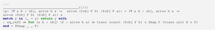
  Obviously, such a p exists as eq_refl. The rest of the proof follows from the coherence conditions provided by the adjunction A under the functional extensionality assumption.

It now remains to implement the fact that the functor L is unique in order to get the whole proof formalized in Coq. For that, we start with implementing a helper statement as in Lemma 2.6:

In the above proof script, we first build the equation trans eps b o fmap F (fmap G g o eta a) = trans eps b o fmap F (fmap G g o eta a) by subsequent applications of f_equal to the equation fmap G g o (trans eta a) = fmap G h o (trans eta a) named Hh. Then, using the naturality of eta and one of the coherence conditions of the adjunction A we close the goal.

It finally comes to summarize how the unicity proof is formalized in Coq:

It is indeed an equality proof between functors L and R which proceeds with an application of F_split. This gives us two sub-goals to discharge: (1) they map objects and (2) morphisms in the same way. The former trivially follows from the definition of L and the assumption FT o R = F. In the proof of the latter, we follow similar steps with the one of commL in such a way that we need to successfully tackle the heterogeneous equality as the second enumeration above. We use the UIP axiom since L and R map arrow in the same way only contextually not judgmentally. We end up with a goal of the following shape: trans counit (fobj F b) o fmap F f = fmap a b f, for all $\mathtt {f:a \rightarrow GFb}$ in C (natively $\mathtt {f^\flat :a \rightarrow b}$ in CK). We then apply the helper lemma adj_unique_map and get two goals: f = fmap G (trans counit (fobj F b) o fmap F f) o trans unit a and f = fmap G (fmap a b f) o trans unit a. The proofs of both goals follow from the coherence conditions of the adjunction A1. Finally, we state the comparison theorem and prove it in Coq:

The goal simply gets discharged by providing an existence of such a comparison functor followed the application of the fact that the functor makes the proof diagram commutative in both directions, and finally showing the fact that it is unique.

4 Conclusion

The categorical setting in which a comonad determining a coKleisli adjunction with a monad over a Kleisli adjunction is used as an interpretation environment to formalize the state effect by Duval. See Fig. 2. The state-effect-triangles, as in Fig. 1, by Jacobs also provide a categorical setting to interpret the state effect. Mac Lane’s comparison theorem plays an important role in both approaches. In the former, the provided unique comparison functor annihilates the “dual” adjunctions and serves a better understanding of modifier terms. While in the latter, the comparison functor directly interprets a map that maps programs to some predicates that describe their actions during the computations. For example, it may be seen as the weakest precondition functor which maps programs to their weakest preconditions given any post-condition.

We have formalized in Coq the comparison theorem for the Kleisli construction together with the use case given in Example 3. We also showed that the foundations we use are equivalent to the foundations of Timany. Our formalization currently suffices to analyze Duval’s approach but only the one half of the approach by Jacobs. To build on this, we plan to continue with formalizing a proof of comparison theorem for the monad algebras in Coq. This is a variant of the comparison theorem for the Kleisli construction in such a way that the Kleisli category $\mathscr {C}_T$ of the monad T is replaced with the Eilenberg–Moore category $\mathscr {C}^T$ of algebras of T. This will then give a complete picture of the state-effect triangles by Jacobs in a Coq formalization. Beck’s monadicity theorem [14, Ch. VI, §7, Theorem 1] constitutes a next possible challenging formalization goal.

Appendix A. Organization of the Coq Sources

In the accompanying library you will find 9 Coq source files. The following 8 files are indeed relevant for the proof of the comparison theorem and its use case (Example 3): Imports, Category, Functor, NaturalTransformation, Monad, Adjunction, Comparison and UseCase. They are given in an order such that subsequent one always depends on the previous ones. I.e., UseCase depends on all files.

The remaining file, namely equivalence, includes the equivalence proofs of the overlapping parts of our library with the one of Timany [20].

We have named in the implementation the lemma/theorem and definition statements as they appear in the paper. Below we provide information about which statement is located in which file:

$\bullet$Functor.v: Functor (class), F_split (lem).

$\bullet$NaturalTransformation.v: NaturalTransformation (cls).

$\bullet$Monad.v: Monad (class), Kleisli_Category (def), FT (def), GT (def).

$\bullet$Adjunction.v: Adjunction (class), adj_mon (thm), adj_comon (thm), mon_kladj (thm),adj_unique_map (lem).

$\bullet$Comparison.v: L (def), commL (lem), uniqueL (lem), ComparisonMacLane (thm).

$\bullet$UseCase.v: Example 3 as AnniliationOfDualAdjunctions (thm).

The sources have been tested to compile fine with coqc versions 8.7.2, 8.8.0, 8.8.1 and 8.8.2 within approximately 7 seconds on an Intel Core i7-7600U machine with 20GB external memory, and running Ubuntu 18.04 LTS.

References

Bauer, A., Pretnar, M.: Programming with algebraic effects and handlers. J. Log. Algebr. Methods Program. 84(1), 108–123 (2015)
Byliński, C.: Introduction to categories and functors. Form. Math. 1(2), 409–420 (1990)
Capriotti, P.: pcapriotti/agda-categories. https://github.com/pcapriotti/agda-categories/, (2014)
Carette, J., Hu, J., Stucki, S., Sebe, MO: agda/agda-categories. https://github.com/agda/agda-categories (2019)
Domínguez, C., Duval, D.: Diagrammatic logic applied to a parameterisation process. Math. Struct. Comput. Sci. 20(4), 639–654 (2010)
Dumas, J.-G., Duval, D., Fousse, L., Reynaud, J.-C.: Decorated proofs for computational effects: States. In: Golas, U., Soboll, T. (eds.), Proceedings Seventh ACCAT Workshop on Applied and Computational Category Theory, Tallinn, Estonia, 1 April 2012, Vol. 93 of EPTCS, pp. 45–59 (2012)
Dumas, J.-G., Duval, D., Fousse, L., Reynaud, J.-C.: A duality between exceptions and states. Math. Struct. Comput. Sci. 22(4), 719–722 (2012)
Ekici, B.: Towards Mac Lane’s Comparison Theorem for the (co)Kleisli construction in Coq. In: Proceedings of the 3rd FMM 2018, co-located with the 11th CICM (2018)
Gross, J., Chlipala, A., Spivak, D.I.: Experience implementing a performant category-theory library in Coq. In: Klein, G., Gamboa, R. (eds.), Interactive Theorem Proving—5th International Conference, ITP 2014, Held as Part of the Vienna Summer of Logic, VSL 2014, Vienna, Austria, July 14–17, 2014. Proceedings, Vol. 8558 of LNCS, pp. 275–291. Springer (2014)
Hoare, C.A.R.: An axiomatic basis for computer programming. Commun. ACM 12(10), 576–580 (1969)
Ishii, H.: konn/category-agda. https://github.com/konn/category-agda, (2013)
Jacobs, B.: A recipe for state-and-effect triangles. Log. Methods Comput. Sci. 13(2) (2017)
Lucassen, J.M., Gifford, D.K.: Polymorphic effect systems. In: Proceedings of the 15th ACM SIGPLAN-SIGACT Symposium on Principles of Programming Languages, POPL ’88, pp. 47–57, New York, NY, USA (1988). ACM
Mac Lane, S.: Categories for the Working Mathematician. Number 5 in Graduate Texts in Mathematics. Springer, Berlin (1971)
McBride, C.: Elimination with a motive. In: TYPES, Vol. 2277 of Lecture Notes in Computer Science, pp. 197–216. Springer (2000)
Moggi, E.: Notions of computation and monads. Inf. Comput. 93(1), 55–92 (1991)
Peebles, D.: copumpkin/categories. https://github.com/copumpkin/categories, (2018)
Plotkin, G.D., Pretnar, M.: Handling algebraic effects. Log. Methods Comput. Sci. 9(4) (2013)
Pouillard, N.: crypto-agda/crypto-agda. https://github.com/crypto-agda/crypto-agda/tree/master/FunUniverse (2015)
Timany, A.: amintimany/categories. https://github.com/amintimany/Categories (2017)
Timany, A., Jacobs, B.: Category theory in Coq 8.5. In: Proceedings of the 1st FSCD, Porto, Portugal, pp. 30:1–30:18 (2016)
Voevodsky, V., Ahrens, B., Grayson, D., et al.: UniMath—a computer-checked library of univalent mathematics. https://github.com/UniMath/UniMath (2018)
Wiegley, J.: jwiegley/category-theory. https://github.com/jwiegley/category-theory (2018)
Acknowledgements
Open access funding provided by University of Innsbruck and Medical University of Innsbruck.
Author information
Authors and Affiliations
Corresponding author
Additional information
Publisher's Note
Springer Nature remains neutral with regard to jurisdictional claims in published maps and institutional affiliations.
This work has been supported by the ERC Grant No. 714034 SMART.