Singular value decomposition in extended double precision arithmetic

Abstract

A well-known and successful algorithm to compute the singular value decomposition (SVD) of a matrix was published by Golub and Reinsch (Numer. Math. 14:403–420, 1970), together with an implementation in Algol. We give an updated implementation in extended double precision arithmetic in the C programming language. Extended double precision is native for Intel x86 processors and provides improved accuracy at full hardware speed. The complete program for computing the SVD is listed. Additionally, a comprehensive explanation of the original algorithm of Golub and Reinsch (Numer. Math. 14:403–420, 1970) is given at an elementary level without referring to the more general results of Francis (Comput. J. 4:265–271, 1961, 1962).

1 Introduction

The IEEE floating point standard, chiefly designed by William Kahan, recommends that hardware implementations should provide an extended precision data format. This is put into effect for x86-64 processors, which provide a native 80-bit extended double precision data format. Higher precisions will be provided in the future [4, p. 43]. In 80-bit extended double precision data format, the significand comprises 64 bits and thus 11 bits more than does the standard IEEE double precision format. In the C programming language, the type specifier long double is reserved for declaration of extended double precision variables. Some compilers, like the GNU compiler, Clang, and Intel’s C/C++ compiler, implement long double using 80-bit extendend double precision numbers on x86-architectures. Extended double precision thus becomes easily available for computations and should be used, as it offers improved accuracy at full computational speed. We give a C implementation of the singular value decomposition (SVD) in extended double precision arithmetic. The program ist based on the algorithm published by Golub and Reinsch in [3].

Let $A\in \mathbb {R}^{m,n}$ a real m × n matrix, let $\ell :=\min \limits \{m,n\}$. It is well known that

$$ A=U{\Sigma} V^{T} $$

(1)

where $U\in \mathbb {R}^{m,m}$, ${\Sigma }\in \mathbb {R}^{m,n}$, and $V\in \mathbb {R}^{n,n}$ such that

$$U^{T}U=I_{m},\quad V^{T}V=I_{n}\quad\text{and}\quad{\Sigma}_{i,i}=\sigma_{i}, i=1,\ldots,\ell,$$

all other elements of Σ being zero. The numbers σ₁,…, σ_ℓ are the non-negative square roots of the ℓ largest eigenvalues of A^TA. We shall assume that

$$\sigma_{1}\geq\sigma_{2}\geq\ldots\geq\sigma_{\ell}\geq0.$$

The computation of U, V, and Σ splits into two parts. The first part is a reduction of A to a bidiagonal matrix. The second part is an implicit application of the QR algorithm (with shifts) to this bidiagonal matrix. We describe bidiagonalization in Section 2. Section 3 is a reminder about the QR algorithm for tridiagonal symmetric matrices and gives an elementary explanation of Francis’ method to use implicit shifts. Section 4 explains how QR steps can implicitly be performed on a bidiagonal matrix. Section 5 gives details on how to compute the shift parameter reliably and Section 6 gives a stopping criterion for the QR iteration. Section 7 outlines how to arrange for computations in extended precision and in Section 8, a complete C function for computing the SVD is given. Test cases are investigated in Section 9 and we conclude in Section 10.

2 Bidiagonalization

A = (a_{i, j}) is a real matrix with m rows i = 0,…, m − 1, counting down from top to bottom, and with n columns j = 0,…, n − 1, counting across from left to right.

With the pair of rows 0 and i = 1,…, m − 1 we do the plane rotations from left

$$ a_{0,j}=\cos \cdot a_{0,j}\ +\ \sin \cdot a_{i,j}, a_{i,j}=-\sin \cdot a_{0,j}\ +\ \cos \cdot a_{i,j}, j=0,\ldots,n-1 $$

overwriting the old with the new values.¹ We choose $\cos \limits$ and $\sin \limits$ as follows: let $p:=a_{0,0},\ q:=a_{i,0},\ r:=\pm \sqrt {p^{2}+q^{2}}$ with same sign as p, $\cos \limits =p/r$ and $\sin \limits =q/r$. ($\cos \limits =1, \sin \limits =0$ if q = 0). Then a_i,0 gets eliminated, i.e., its new value is 0. Note that plane rotations from left leave the sum of squares in a column invariant. Thus while a_i,0 gets annihilated, $a_{0,0}^{2}$ gets bigger. Indeed, the erasing is more some sort of collecting. After i = m − 1, $a_{0,0}^{2}$ is positive unless A has a zero column. In the same way we do with the pair of columns 1 and j = 2,…, n − 1 plane rotations from right

$$ a_{i,1}=a_{i,1}\cdot \cos\ +\ a_{i,j}\cdot \sin, a_{i,j}=-a_{i,1}\cdot \sin\ +\ a_{i,j}\cdot \cos, i=0,\ldots,m-1 $$

again overwriting the old with the new values.² Thus we do not only generate zeros in the leftmost column but also zeros in the top row after the first two entries, which here are called d₀ and e₁. Plane rotations from right leave the sum of squares in a row invariant, thus ${d_{0}^{2}}+{e_{1}^{2}}>0$ unless there is a zero row.

Such plane rotations either from left or from right in order to erase a selected matrix entry are called Givens rotations. Together, we have the main step number one. More such main steps follow, all a repetition of the first one, but each time with another column and another row less.

Let us assume for the moment that m ≥ n. Then, with n − 1 such main steps we can reduce the matrix A to bidiagonal form B. Ignoring the trivial (zero) rows i = n,…, m − 1, one has

$$ B= \left[\begin{array}{cccccc} d_{0} & e_{1} & & & & \\ & d_{1} & e_{2} & & & \\ & & \cdot & \cdot & &\\ & & & \cdot & \cdot & \\ & & & & d_{n-2} & e_{n-1} \\ & & & & & d_{n-1} \end{array}\right] $$

(2)

With e₀ := 0 each column of B has the same form. The remaining B is quadratic with $\det (B)=d_{0}{\cdots } d_{n-1}$ and $\det (B^{T}\!B)={d_{0}^{2}}{\cdots } d_{n-1}^{2}$.

If required, we accumulate all plane rotations from left in U^T and all plane rotations from right in V. These are orthogonal matrices of order m and n. It is helpful for understanding the coming steps to extend the m × n matrix A to the right by the m × m unit matrix I_m and down by the n × n unit matrix I_n. With these two extensions we have a working area with m + n rows/columns of length m + n. At the beginning it is

$$ \left( \begin{array}{ll} A & I_{m} \\ I_{n} \end{array}\right) $$

where A = UBV^T. After the plane rotations from left and right it is

$$ \left( \begin{array}{ll} B & U^{T} \\ V \end{array}\right) $$

All steps of the second part of the algorithm (to be described below) follow this scheme of applying plane rotations from left and right to further reduce B to diagonal form Σ while updating U^T and V.

The case m < n had been omitted in the Algol program published in [3], but is included now. It is best to consider A^T and to apply the algorithm to the n × m matrix A^T. Anyway, as described in Section 7, a copy of A in extended precision format is needed. At the moment this copy is created, one may as well copy A^T. The C function given in Section 8 does so and then computes V^T instead of U^T and U instead of V. It is easy to take this swap into account when returning the matrices U and V. Therefore, we may continue to assume m ≥ n in the following.

The present version of the SVD uses exclusively plane rotations. All Householder reflections from the version of 1967 [3] have been replaced, although they need only half the number of multiplications. But plane rotations will be needed in the second part of the algorithm and can all be done by calling two functions, viz.

PREPARE() :

to compute the desired values $\cos \limits$ and $\sin \limits$ for the next plane rotation,

ROTATE() :

to apply this plane rotation to a pair of BLA-vectors x[ ], y[ ] (defined by equidistant storage in memory, for example matrix rows, columns, diagonals, or single elements).

As said above, the second part of the algorithm will consist in applying further plane rotations from left and right to B with the goal to reduce B to a diagonal matrix. When e_j = 0 occurs for some index j > 0 (iteration indices are dropped), then the matrix B can be split into two bidiagonal submatrices of order j (rows 0,…, j − 1 of B) and n − j (rows j,…, n − 1 of B), which may be diagonalized independently of each other. At any time, the second part of the algorithm will iteratively diagonalize the southernmost remaining bidiagonal submatrix of B with non vanishing off-diagonal elements. The position of this submatrix is described by two indices ℓ and k, both in the range 0,…, n − 1, defining three diagonal blocks of B, as illustrated in (3):

(3)

Here, ℓ = 0 means an empty first block, and k = n − 1 means an empty third block. The third ”bidiagonal” block in fact already is a diagonal matrix and can be ignored for all further computations, $\lvert d_{k+1}\rvert ,\ldots ,\lvert d_{n-1}\rvert$ are singular values. The middle block with lower row index ℓ and upper row index k is characterized by non vanishing off-diagonal elements e_ℓ+ 1,…, e_k and can be diagonalized independently of the upper bidiagonal block (rows 0,…, ℓ − 1 of B).³ The elements e₁,…, e_ℓ− 1 may be zero or not. After each iteration step taken in the second part, k and ℓ are updated by scanning for zero elements e_j. When k = ℓ = 0, then B is completely diagonalized. When ℓ = k > 0, then e_k = 0, $\lvert d_{k}\rvert$ is a singular value and the trivial 1 × 1 matrix (e_k) may be split off the middle block in (3), thus k will be decremented by 1. When ℓ < k, then one continues to operate on the bidiagonal submatrix of B in rows ℓ,…, k, which will be denoted by

$$ B_{\ell,k}= \left[\begin{array}{cccccc} d_{\ell} & e_{\ell+1} & & & & \\ & d_{\ell+1} & e_{\ell+2} & & & \\ & & \cdot & \cdot & &\\ & & & \cdot & \cdot & \\ & & & & d_{k-1} & e_{k} \\ & & & & & d_{k} \end{array}\right]. $$

(4)

In practice, zero tests must be replaced by tests $\lvert e_{j}\rvert \leq tol$. A proper choice of tol will be discussed in Section 6.

3 Symmetric QR steps with shifts

This section is a reminder about one of the most successful algorithms of Linear Algebra, the QR iteration for the diagonalization of matrices. Heinz Rutishauser invented it in 1961 (then in the form of an equivalent LR iteration). The name comes from the basic iteration step for the matrix to be diagonalized, which is here X =: X⁽⁰⁾:

$$ X^{(i)} =: Q^{(i)}R^{(i)} \text{\ and \ }R^{(i)}Q^{(i)} =: X^{(i+1)}, Q^{(i)} \text{\ orthogonal,}\ \ R^{(i)} \text{\ upper triangular.} $$

The step from X⁽ⁱ⁾ to X^(i+ 1) is a similarity transformation: X^(i+ 1) = Q^(i)TX⁽ⁱ⁾Q⁽ⁱ⁾. All X⁽ⁱ⁾ have the same eigenvalues. The absolute values of these invariant eigenvalues, arranged in decreasing order, play a decisive role in analyzing the asympotic behavior of the sequence X⁽ⁱ⁾. The QR iteration will be applied to the symmetric tridiagonal matrix

$$ X := B^{T}\!B, $$

where B is initially given by (2) and more generally by (4), but in this section it is considered in its own right. To describe a single QR step applied to a tridiagonal symmetric matrix, the iteration index ⁽ⁱ⁾ is dropped. Let

$$ X=X^{(i)}= \left[\begin{array}{ccccc} \delta_{0} & \varepsilon_{1} & & & \\ \varepsilon_{1} & \delta_{1} & \varepsilon_{2} & & \\ \quad\cdot & \quad\cdot & \quad\cdot & &\\ & \quad\cdot& \quad\cdot & \quad\cdot & \\ & & \varepsilon_{n-2}& \delta_{n-2} & \varepsilon_{n-1} \\ & & & \varepsilon_{n-1} & \delta_{n-1} \end{array}\right]\quad\text{and}\quad \overline{X}=X^{(i+1)}. $$

As a consequence of the tridiagonal form, each QR step is rather special:

• (1) Q is a product of n − 1 rotations Q_j in plane (j − 1, j), j = 1,…, n − 1, to eliminate ε_j,

• (2) X stays symmetric and tridiagonal (the minor steps are $\ X \rightarrow {Q_{j}^{T}}XQ_{j}$).

• (3) The number of operations per step is only O(n) rather than O(n³).

• (4) The eigenvalues of X are real and non-negative.

• (5) Also the upper triangular matrix R has only three non-trivial diagonals, see Fig. 1.

  Fig. 1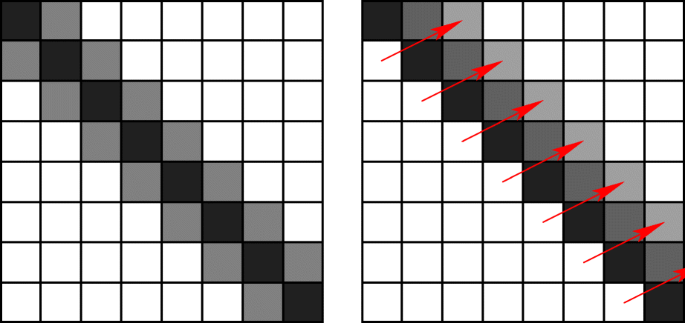

  

  X = B^T B before elimination and R after elimination

The basic iteration step for the QR algorithm with shifts is described as

$$ X-sI =: QR \text{\ and \ }RQ+sI =: \overline{X}, $$

where Q and R are orthogonal and upper triangular, respectively, but not the same as above, depending on the value of s. As before, one has $\overline {X}=Q^{T}XQ$. The value s is called the shift. It should be chosen close to one of the eigenvalues of X. The closer the shift is to such an eigenvalue, the smaller is some diagonal element of R (in most cases the last one) and the smaller is the (last) row and column of $\overline {X}$. Good shifts make Rutishauser’s LR or QR iteration so successful. In [5] Wilkinson proved global convergence of the sequence X⁽ⁱ⁾ to a diagonal matrix for two different strategies to choose a shift. The convergence rate usually is cubic, i.e., for sufficiently small η follows from $\lvert \varepsilon _{n-1}\rvert \leq \eta$ that the next iteration will reduce $\lvert \varepsilon _{n-1}\rvert$ to $O(\lvert \varepsilon _{n-1}\rvert ^{3})$. We devote Section 5 to Wilkinson’s idea and proposals for the shift.

The factorization X − sI = QR and the recombination $QR+sI=\overline {X}$ may be combined to what is known as a QR step with implicit shift. This was found by Francis [1] in a much more general setting, but shall be explained here on an elementary level. Assume that no off-diagonal element of X vanishes, i.e., ε_j≠ 0 for j = 1,…, n − 1. In this case, the orthogonal matrix Q is unique up to a scaling of its columns by ± 1. The matrix Q can always be written as a product of n − 1 rotations Q_j in plane (j − 1, j), j = 1,…, n − 1. The first rotation ${Q_{1}^{T}}$ is to be chosen such that (schematically, just noting the upper 2 × 2-minors)

$$ {Q_{1}^{T}}(X-sI)=\left( \begin{array}{rc} \cos & \sin \\ -\sin & \cos \end{array}\right)\cdot \left( \begin{array}{cc} \delta_{0}-s & \varepsilon_{1}\\ \varepsilon_{1} & \delta_{1}-s \end{array}\right)= \left( \begin{array}{cc} \ast & \ast\\ 0 & \ast \end{array}\right), $$

which is achieved by

$$ \cos=\frac{\delta_{0}-s}{\sqrt{(\delta_{0}-s)^{2}+{\varepsilon_{1}^{2}}}},\quad \sin=\frac{\varepsilon_{1}}{\sqrt{(\delta_{0}-s)^{2}+{\varepsilon_{1}^{2}}}} $$

(5)

(or the negatives of these values). Since ε₁≠ 0, there cannot be a zero division in (5) and moreover $\sin \limits \neq 0$. It is known that

$$ \overline{X}=Q_{n-1}^{T}{\cdots} \underbrace{\left( {Q_{i}^{T}}{\cdots} {Q_{1}^{T}}\cdot A\cdot Q_{1}{\cdots} Q_{i}\right)}_{\displaystyle =:X_{i}} {\cdots} Q_{n-1}. $$

(6)

is tridiagonal, but the matrices X_i, i = 1,…, n − 2, deviate from the tridiagonal form. Schematically, one has

$$ X_{1} = {Q_{1}^{T}}XQ_{1}= \left( \begin{array}{cccccc} \ast & \varepsilon_{1}^{\prime} & \beta_{2} & & & \\ \varepsilon_{1}^{\prime} & \ast & \ast & & & \\ \beta_{2} & \ast & \ast & \varepsilon_{3} & &\\ & & \varepsilon_{3} & \ast & \ast &\\ & & & \ast & \ast & \ast\\ & & & & \ast & \ast \end{array}\right) $$

The extra element β₂ is called bulge element. It is defined by $\beta _{2}=\sin \limits \!\cdot \varepsilon _{2}$ with $\sin \limits$ from (5), so that β₂≠ 0. Now choose a rotation $\tilde {Q}_{2}^{T}$ in plane (1,2), such that multiplication of X₁ from the left with $\tilde {Q}_{2}^{T}$ eliminates β₂ in position (2,0). This is achieved by the choice

$$ \cos=\frac{\varepsilon_{1}^{\prime}}{\sqrt{(\varepsilon_{1}^{\prime})^{2}+{\beta_{2}^{2}}}},\quad \sin=\frac{\beta_{2}}{\sqrt{(\varepsilon_{1}^{\prime})^{2}+{\beta_{2}^{2}}}}. $$

(7)

Schematically, one gets

$$ \tilde{X}_{2} = \tilde{Q}_{2}^{T}X_{1}\tilde{Q}_{2}= \left( \begin{array}{cccccc} \ast & \ast & & & & \\ \ast & \ast & \varepsilon_{2}^{\prime} & \beta_{3} & & \\ & \varepsilon_{2}^{\prime} & \ast & \ast & &\\ & \beta_{3} & \ast & \ast & \ast &\\ & & & \ast & \ast & \ast\\ & & & & \ast & \ast \end{array}\right). $$

The bulge β₂ moved down one position along the diagonal to become $\beta _{3}=\sin \limits \!\cdot \varepsilon _{3}$ with the value $\sin \limits$ defined in (7). Since β₂≠ 0, one has $\sin \limits \neq 0$ again and therefore β₃≠ 0. Continuing this way chasing down the bulge along the diagonal, one arrives at

$$ \tilde{X}_{n-2} = \tilde{Q}_{n-2}^{T}\tilde{X}_{n-3}\tilde{Q}_{n-2}= \left( \begin{array}{cccccc} \ast & \ast & & & & \\ \ast & \ast & \ast & & & \\ & \ast & \ast & \ast & &\\ & & \ast & \ast & \ast & \beta_{n-1}\\ & & & \ast & \ast & \ast\\ & & & \beta_{n-1} & \ast &\ast \end{array}\right) $$

again with β_n− 1≠ 0. A last rotation $\tilde {Q}_{n-1}^{T}$ in plane (n − 2, n − 1) is chosen such that multiplication of $\tilde {X}_{n-2}$ from the left with $\tilde {Q}_{n-1}^{T}$ eliminates β_n− 1 in position (n − 1, n − 3). Then $\tilde {X}_{n-1}=\tilde {Q}_{n-1}^{T}\tilde {X}_{n-2}\tilde {Q}_{n-1}$ is tridiagonal again. Because all bulges are non-zero, all rotations $\tilde {Q}_{i}$, i = 2,…, n − 1, are uniquely determined (up to phase factors, i.e., up to multiplications by ± 1). This means that once Q₁ is set, the need to chase down the bulge until it disappears and to re-establish the tridiagonal form of

$$ \tilde{X}_{n-1}=\tilde{Q}_{n-1}^{T}{\cdots} \tilde{Q}_{2}^{T}\cdot {Q_{1}^{T}}\cdot X\cdot Q_{1}\cdot \tilde{Q}_{2} {\cdots} \tilde{Q}_{n-1} $$

(8)

uniquely determines $\tilde {Q}_{2},\ldots ,\tilde {Q}_{n-1}$ (up to phase factors). But tridiagonal form will also be established by using the rotations Q₂,…, Q_n− 1 as in (6). The conclusion is that $\tilde {Q}_{i}=Q_{i}$, i = 2,…, n − 1 (up to phase factors). The choice of Q₁ according to (5) — which is the only place where the shift explicitly enters the computation — and the choice of $\tilde {Q}_{2},\ldots ,\tilde {Q}_{n-1}$ such as to chase down the bulge, will make (8) an implementation of the QR step.

Thus, the symmetric QR step with shift for the matrix X = B^T B can be done as follows:

• (1) Choose a good shift s.

• (2) Choose ${Q_{1}^{T}}$ according to (5) and compute $X_{1}={Q_{1}^{T}}XQ_{1}$.

• (3) Choose rotations $\tilde {Q}_{j}$ in plane (j − 1, j) in order to chase down the bulge and successively build $X_{j}:=\tilde {Q}_{j}^{T}X_{j-1}\tilde {Q}_{j}$, j = 2,…, n − 1. $\overline {X}:=X_{n-1}$ is the next matrix X.

4 Implicit QR steps on bidiagonal matrix

The QR iteration could explicitly be applied to the matrix X = B^T B with B = B_{ℓ, k} from (4) — the double index of B_{ℓ, k} will be dropped now. The non-trivial diagonal and off-diagonal entries of X then are

$$ \begin{array}{ll} X_{j,j}={d_{j}^{2}}+{e_{j}^{2}}, & \quad (j=\ell,\ldots,k) \quad\text{and}\\[0.2cm] X_{j-1,j}=X_{j,j-1}=d_{j-1}e_{j},&\quad (j=\ell+1,\ldots,k). \end{array} $$

(9)

However, for reasons of economy and accuracy, one should avoid dealing with B^T B. Rather, it is preferable to work with B alone. In fact it is possible to do the similarity transformations on X with two-sided plane rotations, viz. HCode $B \rightarrow {P_{j}^{T}}B Q_{j}$, j = ℓ,…, k − 1, where all matrices Q_j and ${P_{j}^{T}}$ are Givens rotations. To be precise, assume that

$$ d_{j-1}\neq0\quad\text{and}\quad e_{j}\neq0\quad\text{for}\quad j=\ell+1,\ldots,k, $$

(10)

— according to (9) this means that X has no vanishing off-diagonal elements — and choose Q_ℓ as if performing the first minor step of one QR iteration step (with shift) for X. From (5) and (9) it can be seen that this means to choose Q_ℓ as a rotation in the plane (ℓ, ℓ + 1) with

$$ \cos=\frac{d_{\ell}^{2}-s}{\sqrt{(d_{\ell}^{2}-s)^{2}+(d_{\ell}e_{\ell+1})^{2}}},\quad \sin=\frac{d_{\ell}e_{\ell+1}}{\sqrt{(d_{\ell}^{2}-s)^{2}+(d_{\ell}e_{\ell+1})^{2}}} $$

(11)

(or the negatives of these values), depending on the shift parameter s. Multiplying B with Q_ℓ from the right gives (schematically)

$$ B_{\ell+1}^{\prime} := BQ_{\ell}=B\cdot\left( \begin{array}{cr} \cos & -\sin \\ \sin & \cos \end{array}\right)= \left( \begin{array}{ccccc} d_{\ell}^{\prime} & \ast & & & \\ b_{\ell+1}^{\prime} & \ast & e_{\ell+2} & & \\ & & \ast & \ast & \\ & & & \ast & \ast \\ & & & & \ast \end{array}\right). $$

(12)

$B_{\ell +1}^{\prime }$ is no longer an upper bidiagonal matrix because of the bulge element $b_{\ell +1}^{\prime }=\sin \limits \!\cdot d_{\ell +1}$. The bulge element cannot vanish, since $\sin \limits \neq 0$ and d_ℓ+ 1≠ 0, see (10). To eliminate $b_{\ell +1}^{\prime }$, multiply $B_{\ell +1}^{\prime }$ from the left by a rotation $P_{\ell }^{T}$ in the plane (ℓ, ℓ + 1). Up to a phase factor, this rotation must be given by

$$ \cos=\frac{d_{\ell}^{\prime}}{\sqrt{(d_{\ell}^{\prime})^{2}+(b_{\ell+1}^{\prime})^{2}}},\quad\sin=\frac{b_{\ell+1}^{\prime}}{\sqrt{(d_{\ell}^{\prime})^{2}+(b_{\ell+1}^{\prime})^{2}}}, $$

such that (schematically)

$$ B_{\ell+1}:=P_{\ell}^{T}\cdot B_{\ell+1}^{\prime}=\left( \begin{array}{rc} \cos & \sin \\ -\sin & \cos \end{array}\right)\cdot B_{\ell+1}^{\prime}= \left( \begin{array}{ccccc} \ast & \ast & b_{\ell+1} & & \\ 0 & \ast & \ast & & \\ & & d_{\ell+2} & \ast & \\ & & & \ast & \ast \\ & & & & \ast \end{array}\right). $$

(13)

The bulge has moved and becomes $b_{\ell +1}=\sin \limits \!\cdot e_{\ell +2}$. Since $b_{\ell +1}^{\prime }\neq 0$, also b_ℓ+ 1≠ 0. To eliminate b_ℓ+ 1, multiply from the right with a rotation $\tilde {Q}_{\ell +1}$ like in (12), but now in the plane (ℓ + 1, ℓ + 2). Because of b_ℓ+ 1≠ 0, this rotation must have a component $\sin \limits \neq 0$. The multiplication results in

$$ B_{\ell+2}^{\prime} := B_{\ell+1}\tilde{Q}_{\ell+1}= \left( \begin{array}{cccccc} \ast & \ast & 0 & & & \\ & \ast & \ast & & & \\ & b_{\ell+2}^{\prime}& \ast & e_{\ell+3} & &\\ & & & \ast & \ast & \\ & & & & \ast & \ast\\ & & & & & \ast \end{array}\right) $$

with $b_{\ell +2}^{\prime }=\sin \limits \!\cdot d_{\ell +2}\neq 0$. To eliminate the bulge $b_{\ell +2}^{\prime }$, multiply from the left by a rotation $P_{\ell +2}^{T}$ in the plane (ℓ + 1, ℓ + 2). Since $b_{\ell +2}^{\prime }\neq 0$, this rotation once more is uniquely determined (up to a phase factor) with $\sin \limits \neq 0$. One gets

$$ B_{\ell+2}:=P_{\ell+1}^{T}\cdot B_{\ell+2}^{\prime}= \left( \begin{array}{cccccc} \ast & \ast & & & & \\ & \ast & \ast & b_{\ell+2} & & \\ & 0 & \ast & \ast & &\\ & & & d_{\ell+3} & \ast & \\ & & & & \ast & \ast\\ & & & & & \ast \end{array}\right) $$

with $b_{\ell +2}=\sin \limits \!\cdot e_{\ell +3}\neq 0$. Continuing this way the bulge initially introduced by multiplication with Q_ℓ is chased down in knight’s moves until it disappears. This is illustrated in Fig. 2, where the bulge at different moments in the computation is notated as x, $x^{\prime }$, $x^{\prime \prime }$, and $x^{\prime \prime \prime }$. All moves in north-eastern direction are effected by plane rotations from left and all moves in south-western direction are effected by plane rotations from right. The rotations $\tilde {Q}_{\ell +1},\ldots ,\tilde {Q}_{k-1}$ from the right and $P_{\ell }^{T},\ldots ,P_{k-1}^{T}$ from the left are all uniquely determined (up to phase factors) once Q_ℓ is chosen. In the end, with

$$ \tilde{Q}:=Q_{\ell}\cdot \tilde{Q}_{\ell+1}{\cdots} \tilde{Q}_{k-1}\quad\text{and}\quad P:=P_{\ell}\cdot\ldots\cdot P_{k-1} $$

the matrix $P^{T}B\tilde {Q}=:\overline {B}$ is bidiagonal again. Therefore

$$ (\overline{B})^{T}\overline{B}=\tilde{Q}^{T}B^{T}\!B\tilde{Q}=\tilde{Q}^{T}X\tilde{Q} $$

is a tridiagonal matrix again. The first rotation Q_ℓ was explicitly chosen as needed to perform a step of the QR iteration. It was seen in Section 3, that this and the fact that $\tilde {Q}^{T}X\tilde {Q}$ is tridiagonal are enough to conclude that $\tilde {Q}^{T}X\tilde {Q}$ is the result of a full QR step performed on X.

Fig. 2

Chasing the bulge

The conclusion is that one step of the QR iteration (with shift s) for X = B^TB can be done implicitly as follows

• (1) Depending on the chosen shift s set Q_ℓ as in (11), and multiply B from the right with Q_ℓ.

• (2) Multiply with further rotations $\tilde {Q}_{\ell +1},\ldots ,\tilde {Q}_{k-1}$ and $P_{\ell }^{T},\ldots ,P_{k-1}^{T}$ to chase down the bulge until it disappears.

The above arguments depend on (10), but a violation of these conditions even is an advantage, since then savings are possible. In case $\lvert e_{k}\rvert \leq tol$, $\lvert d_{k}\rvert$ is accepted as a singular value and k is decremented by 1. In case $\lvert e_{i}\rvert \leq tol$ for some ℓ ≤ i < k, e_i is neglected and the matrix B is split in two bidiagonal matrices which are diagonalized separately. The saving on d_i = 0 is almost as obvious: one can chase this zero to the right with plane rotations $\hat {P}_{i+1}^{T},\ldots ,\hat {P}_{k}^{T}$ from left in rows i and j = i + 1,…, k, so that the matrix B gets a zero row:

$$ \begin{array}{cccc} \left[\begin{array}{cccccc} \ast & \ast & & & & \\ & \ast & \ast & & &\\ & & 0 & e_{i+1} & &\\ & & & \ast & \ast & \\ & & & & \ast & \ast\\ & & & & &\ast \end{array}\right] & \stackrel{\hat{P}_{i+1}^{T}\cdot}{\longrightarrow} & \left[\begin{array}{cccccc} \ast & \ast & & & & \\ & \ast & \ast & & & \\ & & 0 & 0 & x & \\ & & & \ast & \ast & \\ & & & & \ast & \ast \\ & & & & &\ast \end{array}\right] & \stackrel{\hat{P}_{i+2}^{T}\cdot}{\longrightarrow} \\ \multicolumn{2}{r}{\cdots\stackrel{\hat{P}_{k-1}^{T}\cdot}{\longrightarrow} \left[\begin{array}{cccccc} \ast & \ast & & & & \\ & \ast & \ast & & & \\ & & 0 & {\cdots} & 0 & x^{\prime} \\ & & & \ast & \ast & \\ & & & & \ast & \ast \\ & & & & &\ast \end{array}\right] } & \multicolumn{2}{l}{\stackrel{\hat{P}_{k}^{T}\cdot}{\longrightarrow} \left[\begin{array}{cccccc} \ast & \ast & & & & \\ & \ast & \ast & & & \\ & & 0 & \cdot & \cdot & 0\\ & & & \ast & \ast & \\ & & & & \ast & \ast \\ & & & & &\ast \end{array}\right].} \end{array} $$

Now B can be split in two bidiagonal matrices to be diagonalized separately. In case $\lvert d_{i}\rvert \leq tol$, the effect is the following. Multiplication with $\hat {P}_{i+1}^{T}$ annihilates e_i+ 1 and creates new elements x_i+ 1 in position (i, i + 2) and η_i+ 1 in position (i + 1, i). Multiplication with $\hat {P}_{i+2}^{T}$ annihilates x_i+ 1 (in row i) and creates new elements x_i+ 2 in position (i, i + 3) and η_i+ 2 in position (i + 2, i). Multiplication with $\hat {P}_{k}^{T}$ annihilates x_k− 1 (in row i) and creates η_k in position (k, i). The result is a matrix of the form (all modified elements are overlined)

$$ B=\left[\begin{array}{cccccccc} d_{\ell} & e_{\ell+1} & & & & & &\\ \quad\cdot & \quad\cdot & & & & & &\\ & \quad\cdot & \quad\cdot & & & & & \\ & & \quad\cdot & e_{i} & & & &\\ & & & \bar{d}_{i} & 0 & & &\\ & & & \eta_{i+1} & \bar{d}_{i+1} & \bar{e}_{i+2} & &\\ & & & \cdot & \quad\cdot & \quad\cdot & & \\ & & & \cdot & & \quad\cdot & \quad\cdot & \\ & & & \cdot & & & \quad\cdot & \bar{e}_{k}\\ & & & \eta_{k} & & & & \bar{d}_{k} \end{array} \right]. $$

By the orthogonality of plane rotations

$$\bar{d}_{i}^{2}+\eta_{i+1}^{2}+\ldots+{\eta_{k}^{2}}={d_{i}^{2}}\leq tol^{2},$$

which shows that all elements $\bar {d}_{i},\eta _{i+1},\ldots ,\eta _{k}$ have a magnitude less than or equal tol and can be neglected. B can again be split in two bidiagonal matrices. The case of a vanishing or negligible diagonal element d_i is called cancellation.

5 Choosing a shift

The way shifts are chosen is an essential and characteristic part of the SVD. The shift has only one purpose: to decrease $\lvert e_{k}\rvert$, the last off-diagonal entry in the current iteration matrix B = B_{ℓ, k} (again, the double index (ℓ, k) will be dropped). Remember, that a good shift is close to one of the eigenvalues of the matrix B^T B, which are the squares of the singular values. The non-trivial elements in the last two columns of B are

$$ \left( \begin{array}{ll} e_{k-1} & 0 \\ d_{k -1} & e_{k} \\ 0 & d_{k} \end{array}\right)\ =: \ \left( \begin{array}{ll} g & 0 \\ y & h\\ 0 & z \end{array}\right) $$

One may assume that g, y, h and z are all non-zero, otherwise B would have been split. One of the simplest and most effective choices for the shift is the last diagonal element of B^T B, which is h² + z², one of the Wilkinson shifts, also known as Rayleigh shift. An alternative, used in the original SVD of 1967, is to choose one eigenvalue of the last 2 × 2 diagonal block of B^T B. This choice was originally designed for the cases where one needs a pair of conjugate complex shifts. However, if one needs just one shift, it is mandatory to select the eigenvalue which is closer to h² + z² because the other one could be far away. (Indeed this had been done in [3], but not been pointed out sufficiently.) Then the shift s comes from the quadratic

$$ \det\left( \begin{array}{cc} g^{2} + y^{2} - s\ & \ hy \\ hy\ & \ h^{2} + z^{2} - s \end{array} \right)\ = \ 0. $$

We want the root s which is closer to h² + z², i.e., the root t := h² + z² − s closest to zero of the quadratic

$$ t^{2} + (g^{2} + y^{2} - h^{2} - z^{2})\ t - h^{2}y^{2}\ = \ 0. $$

It is good numerical practice to first compute the larger root t₁ and then the smaller one t₂ from t₁t₂ = −h²y². As h and y are non-zero one can form

$$f := (g^{2}+y^{2}-h^{2}-z^{2})/(2hy)= [(y-z)(y+z)+(g-h)(g+h)]/(2hy).$$

Let $w=\sqrt {f^{2}+1}$, then t has the roots hy(−f ± w). If f > 0, then yh(−f − w) is the one with bigger modulus and t = yh/(f + w) is the one with smaller modulus. If f < 0, then yh(−f + w) is the one with bigger modulus and yh/(f − w) is the one with smaller modulus. The shift to be chosen thus is

$$ s \ = \ z^{2}+h^{2}-hy/(f+w)\quad\text{or}\quad s \ = \ z^{2}+h^{2}-hy/(f-w),$$

for f > 0 or f < 0, respectively. The only place where the shift enters into the computation of the implicit QR step is (11). Evidently the values for $\cos \limits$ and $\sin \limits$ in (11) do not change if $d_{\ell }^{2}-s$ is replaced by d_ℓ − s/d_ℓ and if d_ℓe_ℓ+ 1 is replaced by e_ℓ+ 1. This fact will be used in the program of Section 8.

For this second choice of shift (called shift strategy (b) in [5]), Wilkinson proved global convergence with a guaranteed quadratic convergence rate. Almost always convergence is cubic, as confirmed by the test cases examined in Section 9. One therefore expects $s \rightarrow z^{2}$ from $h \rightarrow 0$ and y bounded. After convergence, k is decremented until with enough QR steps k = 0 is reached.

6 Test for convergence

When $\lvert e_{k}\rvert \leq tol$, then $\lvert d_{k}\rvert$ is accepted as new singular value and k is decremented by 1. When $\lvert e_{i}\rvert \leq tol$ for some i < k, then the matrix B is split in two parts and the singular values of both parts are computed separately, as said above. The cancellation case $\lvert d_{i}\rvert \leq tol$ was considered in Section 4. It remains to choose the tolerance tol. Here, we repeat the proposal from [3] to choose

$$ tol = {\|B\|}_{\infty}\cdot\epsilon_{\tiny\text{mach}} $$

(14)

with 𝜖_mach the machine precision and B the initial bidiagonal matrix from (2).

7 Extended precision arithmetic

On the preceding pages all algorithmical aspects of computing the real matrices A, U, V, Σ and B have been described without mentioning their common data type. Now we are specific. We assume that a user keeps A stored as a variable in standard IEEE double floating point format and wants to get U, V, and Σ also as variables in double format. We call the corresponding variables external and use lower case letters to notate them. We perform the SVD computation inside a C function SVD in long double extended precision format. This function needs internal copies of data type long double of the external variables. The internal variables shall be denoted by upper case letters. We thus have

matrix	external variable	internal variable
A	a	A
U	u	P or Q
V	v	Q or P
Σ	d	D
B	–	D, E

where the dash in the last line means that B is only computed internally. Its diagonal is stored in D(which will be overwritten by the singular values on the diagonal of Σ) and its superdiagonal is stored in E. Explanations for the internal variables P and Q will be given in a moment.

When SVD is called, at first the C library function malloc is invoked to dynamically allocate memory for the internal variables. Then matrix A is copied from a to A, if m ≥ n. If, however, m < n, then A^T is copied to A, as announced in Section 2. With

$$ma:=\max\{m,n\},\quad mi:=\min\{m,n\},$$

A can always be considered a ma × mi matrix. All rotations from left will be accumulated in P (of dimension ma × ma) and all rotations from right will be accumulated in Q (of dimension mi × mi). As seen in Section 2, at the end of the computation, P holds U^T and Q holds V, if m ≥ n. If, however, m < n, then Q holds U and P holds V^T. Of course, P and Q must be initialized as identity matrices before the accumulations can start.

As already said in the introduction, on the Intel x86 architecture all arithmetic operations are done in 64 bit precision with full hardware speed. Also, the exponent of long double has 15 bits and thus four more bits than are provided for double. Therefore, there will be no problems with exponent overflow or underflow when squaring elements a_{i, j} of A.

At the end of the computation in function SVD, the internal variables are rounded to double format and copied to the external variables a, u, v, and d. This is the moment to copy singular values in descending order from D to d. Columns / rows of P and Q must be copied in corresponding order. Finally the allocated memory for the internal variables must be freed (the 64 bit precision results get lost).

8 C program

An implementation of the SVD in the C programming language is available from the web page https://www.unibw.de/eit_mathematik/forschung/eprecsvd as the na59 package.

In the header file SVD.h one may switch on or off computations in extended double precision and choose between Rayleigh shifts (corresponding to shift strategy (a) in [5]) and Wilkinson shifts (shift strategy (b) in [5]).

The file SVD.c contains an implementation of the SVD algorithm. All constants of data type long double are marked by a suffix W. The printf statements are included for testing only and can be omitted. At the end of SVD a function testSVD is called, which is implemented in SVDtestFunc.c. Its purpose is to test whether the fundamental identities U^TU = I_m, V^TV = I_n and AV = UΣ (nearly) hold. The calling of this function can also be omitted, of course.

The file SVDtest2.c contains an implementation of all the test cases discussed in the following section.

9 Test results

Computations were carried out on an Intel processor i7-9850H, programs were compiled with the GNU compiler, version 10.2.0. The results obtained by computations in extended double precision arithmetic are noted as $\tilde {U}$, $\tilde {V}$ and $\tilde {\Sigma }$. These results were rounded to standard double precision format to give $\hat {U}$, $\hat {V}$ and $\hat {\Sigma }$. The singular values on the diagonal of $\hat {\Sigma }$ are noted as $\hat \sigma _{k}$.

When exact singular values are known, they are rounded to standard double precision format and noted as σ_k. In the cases where exact singular values are not known, numerical approximations were computed via an implementation of the SVD in 256-bit arithmetic, based on the GNU MPFR multiple precision library. The singular values obtained from a multiple precision computation were then rounded to standard double precision format and taken as substitutes for the unknown exact singular values. The abbreviation $\mu (A)=\max \limits \lvert a_{i,j}\rvert$ for a matrix A = (a_{i, j}) is used below.

A first example is taken from [3]. It is the matrix

$$ A=\left[\begin{array}{rrrrr} 22 & 10 & 2 & 3 & 7\\ 14 & 7 & 10 & 0 & 8 \\ -1 & 13 & -1 & -11 & 3 \\ -3 & -2 & 13 & -2 & 4 \\ 9 & 8 & 1 & -2 & 4\\ 9 & 1 & -7 & 5 & -1\\ 2 & -6 & 6 & 5 & 1 \\ 4 & 5 & 0 & -2 & 2 \end{array}\right] $$

(15)

with exactly known singular values

$$\sigma_{1}=\sqrt{1248},\quad\sigma_{2}=20,\quad\sigma_{3}=\sqrt{384},\quad\sigma_{4}=\sigma_{5}=0.$$

After a total of 6 QR iteration steps, the singular values $\hat \sigma _{k}$ from Table 1 were found.

Table 1 Singular values for example matrix (15)

A value of 0 in the second column of Table 1 means that both, exact and computed singular values, are identical after rounding to standard double precision format. The accuracy of the achieved decomposition is characterized by

$$\mu(\tilde{U}^{T}\tilde{U}-I_{m})=3.25_{10} - 19,\quad\mu(\tilde{V}^{T}\tilde{V}-I_{n})=3.25_{10} - 19$$

and

$$\mu(A\tilde{V}-\tilde{U}\tilde{\Sigma})=1.73_{10} - 18.$$

These fundamental identities were checked before the results were rounded to standard double precision by calling the function testSVD from within function SVD.

A second example is the 10 × 7 Hilbert matrix A defined by

$$ a_{i,j}=\frac{1}{i+j-1},\quad i=1,\ldots,10,\quad j=1,\ldots,7. $$

(16)

In this case, exact singular values are not known and substitutes for them were obtained from a computation in 256-bit arithmetic, as described above. After a total of 8 QR iteration steps, the results given in Table 2 were found.

Table 2 Singular values for example matrix (16)

Concerning the fundamental identities, the results

$$\mu(\tilde{U}^{T}\tilde{U}-I_{m})=3.25_{10} - 19,\quad\mu(\tilde{V}^{T}\tilde{V}-I_{n})=3.25_{10} - 19$$

and

$$\mu(A\tilde{V}-\tilde{U}\tilde{\Sigma})=1.08_{10} - 19$$

were obtained.

A third example is taken from [2]. Setting

$$B=\left[\begin{array}{rrrrrr} 5 & -1 & -1 & 6 & 4 & 0 \\ -3 & 1 & 4 & -7 & -2 & -3 \\ 1 & 3 & -4 & 5 & 4 & 7 \\ 0 & 4 & -1 & 1 & 4 & 5\\ 4 & 2 & 3 & 1 & 6 & -1\\ 3 & -3 & -5 & 8 & 0 & 2 \\ 0 & -1 & -4 & 4 & -1 & 3\\ -5 & 4 & -3 & -2 & -1 & 7\\ 3 & 4 & -3 & 6 & 7 & 7 \end{array}\right], $$

an 18 × 12 matrix is defined by

$$ A=\left[\begin{array}{rr} B & 2B\\ 3B & -B \end{array}\right]. $$

(17)

Since this matrix has rank 6, σ₇ = … = σ₁₂ = 0. Substitutes for the exact singular values σ₁,…, σ₆ of A were obtained from a computation in 256-bit arithmetic, as described above. After a total of 12 QR iteration steps, the results shown in Table 3 were found.

Table 3 Singular values for example matrix (17)

Again, the fundamental identities were checked, with the following results:

$$\mu(\tilde{U}^{T}\tilde{U}-I_{m})=5.42_{10} - 19,\quad\mu(\tilde{V}^{T}\tilde{V}-I_{n})=6.51_{10} - 19$$

and

$$\mu(A\tilde{V}-\tilde{U}\tilde{\Sigma})=1.39_{10} - 17.$$

A fourth example is taken from [3]. It is the 20 × 21 matrix defined by

$$ a_{i,j}=\left\{\begin{array}{rl} 0, &\quad\text{if }i>j\\ 21-i, &\quad\text{if }i=j,\\ -1,&\quad\text{if }i<j, \end{array}\right.\quad i=1,\ldots,20,\quad j=1,\ldots,21, $$

(18)

with exact singular values

$$\sigma_{21-k}=\sqrt{k(k+1)},\quad k=1,\ldots,20.$$

The method converged after 39 QR iterations with the results shown in Table 4.

Table 4 Singular values for example matrix (18)

In this example, all values $\lvert \sigma _{k}-\hat {\sigma }_{k}\rvert$ were 0, i.e., computed and exact values were identical, when both rounded to standard double precision. The fundamental identities were checked with the following results:

$$\mu(\tilde{U}^{T}\tilde{U}-I_{m})=1.08_{10} - 18,\quad\mu(\tilde{V}^{T}\tilde{V}-I_{n})=1.73_{10} - 18$$

and

$$\mu(A\tilde{V}-\tilde{U}\tilde{\Sigma})=1.73_{10} - 17.$$

A fifth example is again taken from [3]. It is the 30 × 30 matrix defined by

$$ a_{i,j}=\left\{\begin{array}{rl} 0, &\quad\text{if }i>j\\ 1, &\quad\text{if }i=j,\\ -1,&\quad\text{if }i<j, \end{array}\right.\quad i=1,\ldots,30,\quad j=1,\ldots,30. $$

(19)

Substitutes for the exact singular values were computed numerically in multiple precision arithmetic. The method converged after 48 QR iterations. Again, all values $\lvert \sigma _{k}-\hat {\sigma }_{k}\rvert$ were 0, i.e., computed and exact values were identical, when both rounded to double precision. The fundamental identities were checked with the following results:

$$\mu(\tilde{U}^{T}\tilde{U}-I_{m})=9.76_{10} - 19,\quad\mu(\tilde{V}^{T}\tilde{V}-I_{n})=6.51_{10} - 19$$

and

$$\mu(A\tilde{V}-\tilde{U}\tilde{\Sigma})=3.47_{10} - 18.$$

10 Conclusions

An implementation of the SVD in extended precision arithmetic substantially improves the accuracy of the computed results. This improvement comes at no loss in computational speed, when extended precision arithmetic is native, as for the x86 architecture. Only a minor programming effort is necessary to use the capabilities of extended precision arithmetic and the same program also runs in standard double precision arithmetic. So it is advantageous to use the updated program.

We have also given a full, elementary explanation of the algorithm of Golub and Reinsch. In [3], not all details were fully explained on an elementary level.

References

Francis, J.: The QR transformation. A unitary analogue to the LR transformation. Comput. J. 4, 265–271 (1961, 1962)
Gander, W.: The first algorithms to compute the SVD, https://people.inf.ethz.ch/gander/talks/Vortrag2022.pdf
Golub, G.H., Reinsch, C.: Singular value decomposition and least squares solutions. Numer. Math. 14, 403–420 (1970)
Higham, N.J.: Acuracy and Stability of Numerical Algorithms, 2nd edn. SIAM (2002)
Wilkinson, J.H.: Global convergence of tridiagonal QR algorithm with origin shifts, Lin. Alg. Appl., 409–420 (1968)
Acknowledgements
Professor Christian Reinsch passed away on October 8, 2022. A year before his death he told me (M.R.) he was working on a revision of the SVD algorithm published in 1970 by Golub and himself. Because of his rapidly worsening eyesight he was no longer able to do the work all on his own. I offered my help and took over the programming, testing, and writing of this article. It was his wish that this work should be published under our joint authorship. I am honored by this proposal. I am very thankful for having met and worked with this outstanding mathematician to whom I owe very much.
Funding
Open Access funding enabled and organized by Projekt DEAL.
Author information
Authors and Affiliations
Contributions
Both authors wrote and reviewed the first versions of the manuscript together. C.R. initiated the work and had the principal idea to use extended precision arithmetic. M.R. wrote the C program (based on the Algol version of C.R.), did the testing and added the explanation of the implicit QR algorithm. M.R. wrote and reviewed the final version of the manuscript and is responsible for all errors.
Corresponding author
Ethics declarations
Ethical approval
Not applicable
Competing interests
The authors declare no competing interests.
Additional information
Publisher’s note
Springer Nature remains neutral with regard to jurisdictional claims in published maps and institutional affiliations.
Rights and permissions
This article is published under an open access license. Please check the 'Copyright Information' section either on this page or in the PDF for details of this license and what re-use is permitted. If your intended use exceeds what is permitted by the license or if you are unable to locate the licence and re-use information, please contact the Rights and Permissions team.
About this article
Cite this article
Reinsch, C., Richter, M. Singular value decomposition in extended double precision arithmetic. Numer Algor 93, 1137–1155 (2023). https://doi.org/10.1007/s11075-022-01459-9
Received:
Accepted:
Published:
Issue Date:
DOI: https://doi.org/10.1007/s11075-022-01459-9