
Abstract
The influence of the internal structure of inhomogeneous particles on their radiative properties is an open issue repeatedly questioned in many fields of science and technology. The importance of a refined description of the particle composition and structure, going beyond mean-field approximations, is generally recognized. Here, we focus on describing internal inhomogeneities from a statistical point of view. We introduce an analytical description based on the two-point density-density correlation function, or the corresponding static structure factor, to calculate the extinction cross sections. The model agrees with numerical predictions and is validated experimentally with colloidal aggregates in the 0.3–6 μm size range, which serve as an inhomogeneous model system that can be characterized enough to work without any free parameters. The model can be tightly compared to measurements with single particle extinction and scattering and spectrophotometry and suggests a simple behavior for 90° scattering from fractal aggregates as a function of extinction, which is also confirmed experimentally and numerically. We also discuss the case of absorbing particles and report the experimental results for water suspensions of black carbon for both the forward and 90° scattering properties. In this case, the total scattering and the extinction cross sections determine the single scattering albedo, which agrees with numerical simulations. The three parameters necessary to feed radiative transfer models, namely, extinction, asymmetry parameter, and single scattering albedo, can all be set by the analytical model, with explicit dependence on a few parameters. Results are applicable to radiative transfer problems in climate, paleoclimate, star and planetary formation, and nanoparticle optical characterization for science and industry, including the intercomparison of different optical methods such as those adopted by ISO standards.
Introduction
Dust, powders, and micro- and nanoparticles of natural and anthropogenic origin have been the subject of extensive research due to their ubiquity and potential industrial applications. In particular, the optical properties of dust are paramount in our understanding of a widespread class of systems, such as the influence of eolian dust on climate balance and remote sensing (Mishchenko et al. 1995; Claquin et al. 1998; Bigler et al. 2011; Kemppinen et al. 2015; Wu et al. 2016; Doner and Liu 2017), dust grains in the solar system, protoplanetary accretion disks, and star-forming clouds (Bazell and Dwek 1990; Kozasa et al. 1992; Stognienko et al. 1995; Fogel and Leung 1998; Voshchinnikov et al. 2000; Shen et al. 2008; Köhler et al. 2011; Ormel et al. 2011; Kataoka et al. 2014; Min et al. 2016). Other examples range from the systems at the nanoscale exploited for emerging bottom-up approaches to pharmaceutics and drug delivery (Rossi et al. 2002; Hertlein et al. 2008; Bonn et al. 2009) to the large scale of cosmic intergalactic dust (Ysard et al. 2015). In some cases, optical properties can be responsible for driving physical and chemical processes that modify dust, impacting on emissivity, temperature, or composition (Henning and Stognienko 1996; DeMott et al. 2003; Draine 2003; Kaufman et al. 2005; Ricci et al. 2010; Miotello et al. 2012).
Three general cases where optical properties are the cornerstones of the analysis can be identified:
-
i)
Interpreting data from optical instruments based on the measurement of light emitted by one or a collection of particles
-
ii)
Interpreting data from light scattering in dust clouds
-
iii)
Modeling physical systems where the light is emitted, scattered, and possibly absorbed by dust grains
Essentially, dust’s radiative properties rely on the size distribution and chemical composition of the grains. However, it is generally accepted that even a precise knowledge of the size and polarizability of the components of a particle is far from being enough to estimate its optical properties; this applies especially to particle sizes close to the radiation wavelength (Nousiainen et al. 2011; Ysard et al. 2018; Walters et al. 2019). Many parameters introduce considerable effects: shape, and therefore orientation, surface roughness and coating (Drossart 1990), internal structure, porosity, and fluffiness (Mattila 1970; McGuire and Hapke 1995; Lehtinen and Mattila 1996; Foster and Goodman 2005; Pagani et al. 2010; Steinacker et al. 2015). For example, absorption in a dust grain is a property for which its chemical composition only gives a rough estimate, mainly due to the influence of surface and density inhomogeneities. Similarly, changes in the optical properties of dust grains due to their internal structure depend on whether they are dielectric or absorbing (Voshchinnikov et al. 2000; Sorensen 2001; Bohren and Huffman 2008; Sorensen et al. 2018).
The introduction of numerical computation tools such as the T-matrix (Mishchenko et al. 2013) or the discrete dipole approximation (DDA) (Purcell and Pennypacker 1973; Penttilä et al. 2007; Yurkin and Hoekstra 2011; Liu et al. 2018), as well as technology advancements, brought a significant increase in precision and a decrease in computing time. However, in real cases, dust is intrinsically multi-component, evolving with time, and highly polydisperse in size, so that computations should be steadily updated. The current uncertainties about the effects of eolian dust on the Earth atmosphere provide a good example: the time evolution of size, coating, and internal mixing is demanding in terms of numerical simulations (Stocker et al. 2013). The problem of assigning optical properties to dust clouds is, therefore, often simplified: particles are modeled as spheres following the Lorenz-Mie approach, and the particle polarizability is approximated by assuming the mean-field approximation (MFA) (Chylek et al. 1988; Bohren and Huffman 2008) or by using standard optical parameters (e.g., see Albani et al. (2014) and references therein). Alternatively, introducing parametrizations that are numerically much cheaper than the Mie expansion can strongly reduce computation times (Ghan and Zaveri 2007). However, many authors have called into question the validity of these assumptions, concluding that they should be discussed for each specific case (Pollack and Cuzzi 1980; Mishchenko et al. 1995; Nousiainen et al. 2011; Sorensen et al. 2018).
In this work, we discuss the effects of internal structures on the main optical properties of scatterers composed by several submicron components. In Sect. 2, we introduce an analytical model relying on a statistical description of the two-point correlation function of the polarizability within the scatterer and compare it to standard approaches in the existing literature. We focus on the extinction and scattering cross sections and the angular distribution of the scattered intensity, providing evidence that the whole set of parameters needed to feed the radiative transfer models can be obtained. With this analytical approach, it is possible to reduce the computation time to a minimum while keeping the explicit dependence on parameters such as the wavelength λ.
In Sect. 3, we use the model to describe the scattering properties of fractal structures composed by spherical monomers. This system is produced under well-controlled conditions, is general enough to be of interest as a case example for many applications, and can be fully characterized with optical methods.
We compare three approaches to describe the aggregates (see Fig. 1):
-
i)
The fractal structure
-
ii)
A hybrid model where each aggregate is described as a collection of randomly distributed monomers (i.e., neglecting the arrangement of the monomers)
-
iii)
The mean-field approximation (MFA) or Maxwell-Garnett (MG) model
Fig. 1 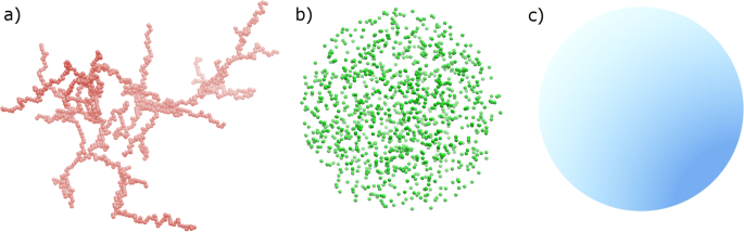
Schematic of the morphologies used for simulations and the analytical model in Figs. 3,4, 5, and 6: (a) fractal aggregate (here N = 1150, a = 0.05 μm, Rg = 2.45 μm, and df = 1.77); (b) corresponding cluster of uncorrelated monomers of radius R = Rg and same a, N; and (c) equivalent homogeneous sphere following the mean-field approximation with R = Rg

The same structures have been characterized with extensive numerical simulations, described in Sect. 4, with many parameters kept under control. We made use of the discrete dipole approximation code ADDA (Yurkin and Hoekstra 2011) for calculating the optical properties for hundreds of thousands of aggregates over an extended size range, from tens to thousands of monomers, with given internal structures and optical properties of the monomers. We compare the predictions of the models and the results of numerical simulations to experimental data in Sect. 5. On the theoretical side, we compare our model to the Rayleigh-Gans-Debye (RGD) description, showing that our model can be considered an extension of a modified Carr-Hermans method introduced some years ago to describe the turbidity of a fractal system based on low angle light scattering (LALS) (Ferri et al. 2015). On the experimental side, we validated the model by comparing it to measurements of water suspensions of colloidal fractal aggregates; the samples have been studied with LALS (Ferri et al. 1988, 2004; Carpineti et al. 1990; Fernández-Barbero et al. 1996) and near-field scattering (NFS) (Mazzoni et al. 2013; Cremonesi et al. 2020b), providing the static structure factor and the phase lag of the scattered waves (Potenza et al. 2010a). These measurements combined provide an overconstrained set of parameters whereby to test the model predictions without any free parameters. Specifically, we measure the complex amplitude of the forward scattered field, S(0), with the SPES method (Potenza et al. 2015c), and the 90° scattered flux, F(90), integrated over a solid angle Ω ≃ 0.3 sr, as described in detail in Cremonesi et al. (2020a). We also measured the spectral extinction, Cext(λ), of a suspension of aggregates with a UV-VIS-NIR spectrophotometer (Shimadzu 1900). We conclude the experimental section by reporting the results from a water suspension of uncalibrated black carbon aggregates, fitting our model to experimental data. We finally discuss applications and perspectives in Sect. 6, which is devoted to the conclusions.
Analytical model
In this section, we aim at describing a variety of cases, including fractal aggregates, which represent a model aggregate system to be experimentally compared to the predictions of theoretical models. We report the fundamental relations for the complex amplitude of the forward scattering, S(0), by extending the expressions reported in Parola et al. (2014) to include the effects of correlations for the scattering of an incident plane wave. The relevance of this quantity lies in the fact that it is related to the total extinction cross section, Cext, by the optical theorem (Newton 1976; Van de Hulst 1981).
where k = 2πn0/λ is the wavenumber of the incident radiation, λ the radiation wavelength in vacuum, and n0 is the refractive index of the surrounding medium. Hence, Cext is proportional to the real part of the complex dimensionless amplitude of the forward scattering, a quantity that can be measured with the SPES method (Potenza et al. 2010b, 2015c). The reader might also refer to Table 2 in the Supplementary Material, where we summarize the nomenclature used in this work. The model we introduce hereafter gives the S(0) of particles with structural inhomogeneities, statistically described by the two-point correlation function of the microscopic polarizability, which in turn is related to the static structure factor, Ss(q).
Let \( \alpha ={a}^3\frac{m^2-1}{m^2+2} \) be the (complex) polarizability of a particle falling in the Rayleigh regime, which we can assume to be a spherical monomer of radius a. The forward scattering amplitude for an ensemble of N primary particles can be expanded to second order in the dimensionless term αk3, while α is related to its relative refractive index, n, by the Clausius-Mossotti equation, where m = n/n0. The analytical derivation reported in the Supplementary Material gives the following result:
Factors C1 and C2 are independent of α and N and result from integrating the form factor of the monomer, P(qa), and the static structure factor of the aggregate, Ss(q) as follows:
where the integration variable is x = q/2k. We highlight that the first term in Eq. (2) does not depend on the structure of the particle and corresponds to assuming that the scattering amplitudes of all the non-interacting dipoles add coherently; i.e., the aggregate behaves as a single dipole of polarizability Nα. In this respect, there is a manifest similarity with the Rayleigh and the Rayleigh-Gans scattering (Van de Hulst 1981; Bohren and Huffman 2008; Villa et al. 2016). The effects of spatial correlations between monomers only appear in the second-order expansion terms: C1 and C2 depend on the size of the aggregate and the arrangement of the primary particles in the aggregate.
From Eqs. (1) and (2), we can derive the expression for the extinction cross section of aggregates with a given statistical description of the corresponding form and structure factors. It is straightforward to separate the real and imaginary part for purely dielectric particles. While \( \operatorname{Im}\ S(0) \) contains both first- and second-order terms in Nαk3, \( \operatorname{Re}\ S(0) \) is given by the second-order term only. Correlations do not affect \( \operatorname{Im}\ S(0) \) appreciably, while they play a major role in \( \operatorname{Re}\ S(0) \), and Cext = 4πC1(Nαk3)2. The case of dielectric particles is particularly significant: the first-order term alone would not be enough to describe scattering, since it would give a paradoxical Cext = 0 (Van de Hulst 1981).
Theoretical models
In the following section, we detail the expression in Eq. (2) for different choices of Ss(q) and discuss how the physical description of the internal structure of the aggregate or cluster affects the real part of S(0). The model predictions are in good agreement with experimental and numerical results in all cases (see Results). The behavior of \( \operatorname{Im}\ S(0) \) versus \( \operatorname{Re}\ S(0) \) for a set of particles with different morphologies, but characterized by the same parameters, is studied below.
Fractal aggregates
The model in Eq. (2) is validated with experimental results obtained with colloidal aggregates formed under controlled conditions (Schaefer et al. 1984) that allow constraining the model predictions without any free parameter. Fractal aggregates have been studied for decades with optical methods, which provide precise measurements of the structure factor, Ss(q), such as LALS in colloidal physics (Weitz and Lin 1986; Lin et al. 1989; Carpineti et al. 1990; Ferri et al. 2004). As discussed in the literature (Sorensen 2001), the structure factor can be fitted by several functions that depend on a small set of parameters, such as the number of primary particles (N), the fractal dimension (df), and the gyration radius (Rg). These parameters occur in a scaling relationship that summarizes the fractal nature of such aggregates (Bushell 2002). If all the primary particles are of the same size, this relation reads:
where a is the radius of the primary particles (monomers) and k0 is a constant prefactor of the order of unity, which in turn is related to df (Sorensen and Roberts 1997; Gmachowski 2002).
In this work, we have characterized the static structure factor of fractals by LALS and NFS measurements, which provide us with a statistical description of Ss(q) as required by our model, and we use standard calibrated polystyrene spheres; thus, P(qa) is determined.
In general, knowing Ss(q) is not enough to also extract Cext, except for purely dielectric particles. We note that Csca(λ) = Cext(λ) if absorption in the system is negligible. This case is at the core of a modified Carr-Hermans method (Carr and Hermans 1978) aimed at studying the spectral extinction of a network of scatterers, namely, fractal aggregates and fibrin gels (Ferri et al. 2015). Similarly to what is reported here, such a model relies on Ss(q) to describe the internal structure of the system. The structure factor was characterized independently with LALS while also taking into account the radiative properties of the structures. The turbidity, strictly related to the average Csca(λ), was measured with a spectrophotometer and compared with LALS turbidimetry data overall the visible spectrum.
In this picture, the Debye model gives a practical expression for evaluating the scattering cross section:
where \( x=\sin \frac{\theta }{2} \). Notably, this result is formally the same following from Eq. (2) if the polarizability is real.
The structure factor appearing in Eqs. (3) and (5) is related to the scattering phase function,\( p\left(\theta \right)=\frac{{\left|S\left(\theta \right)\right|}^2}{k^2{C}_{\mathrm{sca}}} \). What is relevant about this quantity is that, according to the RGD approximation, Ss(q) gives the light scattering differential cross section. From this, the asymmetry parameter, g = 〈∫p(θ) cos θdΩ〉, is obtained by its definition, evaluating the integral over the whole solid angle and taking an orientational average (Chandrasekhar 1960; Mishchenko 1994; Andrews et al. 2006; Emde et al. 2016).
The appropriate expression of Ss(q) has been discussed extensively in the literature, and several proposals have been put forward (Sorensen 2001). All the available analytical expressions have some features in common: they are almost flat at qRg ≪ 1 and follow a power law at qRg ≫ 1 behaving as \( {\left(\mathrm{q}{R}_{\mathrm{g}}\right)}^{-{d}_{\mathrm{f}}} \). In the case of sparse aggregates, the Debye formula gives an analytic expression for Ss(q), which also includes rotational averages:
where the indexes run over the number of monomers i, j = 1, …, N.
In view of a general approach that does not rely on numerical simulations, internal inhomogeneities can be easily described statistically by adopting the static structure factor. Here, we refer to the form given by Sorensen et al. (2018):
where F1, 1 is the hypergeometric function. Using this expression in Eq. (2) gives rise to an interestingly simple relationship between \( \operatorname{Re}\ S(0) \) and \( \operatorname{Im}\ S(0) \) since they both scale almost linearly with N. This is not straightforward from Eqs. (2) and (7); therefore, we can use a simplified form of Eq. (7) for the sake of clarity. Let us roughly represent Ss(q) by the expression (Sorensen 2001):
where the first contribution is the self term due to scattering from single monomers, while the second term accounts for the scattering from pairs of monomers. By taking \( \frac{N-1}{N}\sim 1 \) and kRg → ∞, we obtain
where a1 and a2 only depend on ka, while b1 and b2 are dimensionless functions depending on ka and df, but not on Rg. In our case (k = 13.18 μm−1, a = 0.05 μm, df = 1.75), they assume the values a1 = 0.56, a2 = 1.067, b1 = 4.22, and b2 = 4.03. Notice that the term proportional to b2 in Eq. (9a) vanishes as Rg/a ≫ 1: ReS(0) scales almost linearly with N; thus, \( \mid \operatorname{Im}\ S(0)\mid \) is proportional to \( \operatorname{Re}\ S(0) \). Notably, this relationship does not depend on the fractal dimension, as opposed to the case of the MFA (see below).
In the previous case, we restricted to particles with real polarizability to compare the model predictions to the measurement of non-absorbing colloidal particles. However, the model in Eq. (2) can satisfactorily describe particles with complex polarizability as well, provided that the dimensionless polarizability, which acts as an expansion term, is small: ∣α k3 ∣ ≪ 1. It is the case of strongly absorbing fractal aggregates such as soot. Since these particles have a fractal morphology, we can use the expression in Eq. (7) and introduce the appropriate complex polarizability. Here, we consider n = 1.8 + i 0.3 (see Fig. 6 below), which gives αk3 = 0.014 + i 0.008 according to the Lorentz-Lorenz formula. Again, the model foresees a slope close to 1, in good agreement with simulations and experimental data.
Uncorrelated monomers
To move towards a simpler picture of an aggregate or composite particle, we introduce a set of N uncorrelated, non-overlapping monomers of radius a, and polarizability α, randomly distributed within a sphere of radius R = Rg, where Rg is the radius of gyration of the corresponding fractal particle. Although the arrangement of the monomers in the aggregate is disregarded, the structure is still characterized by two length scales defined by a and Rg, respectively. In the low-density limit, \( N{a}^3\ll {R}_{\mathrm{g}}^3 \) the structure factor becomes
where the first contribution is the self term related to the scattering from single monomers arising from the non-overlapping condition as in the case of fractals, while the second is the distinct term and refers to the scattering from pairs of monomers confined within the sphere. By inserting Eq. (10) into Eqs. (3) and taking (N − 1)/N~1, we obtain:
where a1 = 0.56 and a2 = 1.067 are the same as in Eq. (9) only depending on ka, whereas a3 depends on both ka and kRgand varies from ~3.3 · 10−2 to ~6.3 · 10−3 for N ranging from 50 and 5000. The two second-order terms appearing in \( \operatorname{Re}\ S(0) \) come from the integral of the corresponding self and distinct terms in Ss(q). While the first term scales as \( N\sim {R}_{\mathrm{g}}^{d_{\mathrm{f}}} \), the second scales as \( {N}^2/{R}_{\mathrm{g}}^2\sim {R}_{\mathrm{g}}^{d_{\mathrm{f}}-2} \) if df < 2 (see Supplementary Material); thus, for large kRg, the first term leads and ReS(0) scales as N. As to \( \operatorname{Im}\kern0.5em S(0) \), the first term is given by the first-order contribution Nαk3 already seen in Eq. (9b), while the second-order term (a2αk3~3.75 · 10−2) arising from the integral is much smaller. Since a2 is independent of Rg, \( \operatorname{Im}\ S(0) \) is proportional to N. Hence, \( \operatorname{Im}\ S(0) \) scales linearly with \( \operatorname{Re}\ S(0) \) for kRg ≫ 1.
Mean-field Approximation: the Maxwell-Garnett model
Finally, it is instructive to quantitatively compare the previous cases to the predictions of the MFA, perhaps the most widespread approach in many applications. This approximation gives an estimate of the effective polarizability of any internally mixed, non-compact, or non-homogeneous particle (Markel 2016). Depending on the specific hypotheses and field of application, it is named Maxwell-Garnett, Bruggeman, or Lorentz-Lorenz formula. The MG formula is preferred whenever one of the two components is predominant with respect to the other, and therefore acts as a matrix in which particles are embedded. Fractal aggregates can be regarded as a volume of water (or air) that includes many monomers forming branches (Sorensen 2001). For the sake of convenience, we report the explicit form for the relative refractive index
where m = n/n0 and n0 is the refractive index of the surrounding medium, water in the present case.
In this framework, it is customary to represent the cluster as a homogeneous medium of polarizability Nα, confined within a sphere of radius Rg, as in the previous case (Sorensen 2001). This picture corresponds to the limit ka → 0 while taking N → ∞. From a microscopic standpoint, this is equivalent to separating the molecules of the monomers and spread them homogeneously within a volume defined by Rg. Thus, compared to the previous cases, the information about the monomer radius is lost as is the self-contribution in the definition of the structure factor. Therefore, P(qa) = 1, while the structure factor reduces to Ss(q) = P(qRg), where
Thus, for large clusters (kRg ≫ 1), the integrals in Eq. (3) can be performed analytically, with the result:
where the contribution of correlations to the imaginary part is negligible. The following scaling relation can be derived (Sorensen 2001; Potenza and Milani 2014).
This scaling law obtained from the MFA is in open contrast with the result reported above for the aggregates, where \( \operatorname{Re}\ S(0) \) and \( \operatorname{Im}\ S(0) \) are both proportional to the number of monomers and the slope does not depend on df. This discrepancy is a marked qualitative and quantitative difference between the two approaches.
Numerical simulations
We incorporate the results of extensive numerical simulations for S(0), Cext(λ), and F(90) into our analysis, in addition to the model validation against experimental data. In silico fractal structures were generated by using an algorithm similar to Brown et al. (2010) and Ringl and Urbassek (2013) (case 3.1 above, Fig. 1a). Monomers are added sequentially at neighboring, random positions, while chains are randomly branched until the desired number of monomers is reached. Thus, aggregates can be easily grown with the desired fractal dimension that can be tweaked by varying the compactness of the structure. Once the position of every primary particle is set, the particles are discretized in small cubes (see Moteki (2016)), and the scattering amplitudes of the clusters are then computed. Specifically, we made extensive use of the open-source code ADDA, a C99 implementation of the DDA method based on FFTW3 routines (Yurkin and Hoekstra 2011). Following the documentation guidelines, according to which the ratio of dipoles per wavelength (dpl) should be larger than ~ 10|m|, we set dpl = 30.4, 43.4, and 50.6 for monomers 100, 70, and 60 nm in diameter, respectively, resulting in 15.7, 11.0, and 9.4 nm spacing in the dipole lattice, respectively. We generated about 104 in silico aggregates with masses ranging between ~ 50 and ~ 5000 monomers, 100 nm in diameter, and Rg from ~ 0.3 to ~ 6 μm. We ran many MPI ADDA simulations for each given conformation to calculate rotational averages (the case of 70 nm monomers has also been studied); a total of approximately 1018 floating-point operations have been employed to the aim, using the computation cluster at the Physics Department of the University of Milan.
Simulations also give the structure factor of the resulting structures. In Fig. 2, we show the average Ss(q) of a population of particles similar to the one shown in Fig. 1a. The gyration radius of the particles, Rg = 2.45 μm, gives the position of the cutoff and is in good agreement with the Guinier approximation, which gives the low q limit of the spectrum, Ss(q)~1 – q2Rg2/3. As expected, the high q tail of each spectrum (qRg ≫ 1) is affected by the orientation of the aggregate, but variability cancels out when averaging many configurations. The overall trend of the spectrum follows Eq. (7) (dashed line), and the agreement with the approximation in Eq. (8) (blue, dash-dotted line) is still satisfactory, especially at large q. As a cross-check to verify that numerical simulations correctly describe light scattering by fractal aggregates, we recovered the structure factors experimentally: the agreement is very good with both the expected behavior and the experimental LALS and NFS results (Cremonesi et al. 2020b).

Structure factor obtained by averaging upon rotations and statistical conformations of 700 simulated monodisperse fractal structures (N = 1150, Rg = 2.5 μm and df = 1.75), as a function of the dimensionless ratio of the scattering vector q/2k, where k = 2πn0/λ. The slope gives a fractal dimension df = 1.75, which is in good agreement with the average df of the population considered here. The width of the line in the plot (red) indicates the error bars; the curve superimposes with the expression in Eq. (6) (not shown). The data is in good agreement with the structure factor given by Eq. (7) (dashed line), to be compared with the approximation in Eq. (8) (blue, dash-dotted line)
The fractal dimension of each aggregate can be evaluated by counting the number of monomers inside a sphere of increasing radius centered on the center of mass; we find df ≃ 1.75, in agreement with the slope of the structure factors. Interestingly, we can use this comparison also to set the prefactor k0 ≃ 1.2, which agrees with typical values found in the literature (Gmachowski 2002; Lattuada et al. 2003; Heinson et al. 2012). In principle, the fractal dimension can also be calculated by df = ln(N/k0)/ ln(Rg/a). We note that, due to the logarithmic relation, the effect of the prefactor k0 on the fractal dimension is not critical in the present case. For example, assuming k0 = 1 would give a fractal dimension df = 1.8, very close to 1.75.
We also analyze the results of simulations obtained for uncorrelated monomers (case 3.2 above, Fig. 1b). By means of ADDA, we simulated populations of objects with a random distribution of non-overlapping spheres, characterized by the same set of parameters of the corresponding fractal structures, thus changing the monomer spatial distribution only. The filling factor has been calculated from the fractal dimension df and by assuming a spherical shape for the aggregate. With the same criteria, a homogeneous spherical particle deriving from the MG model (case 3.3 above, Fig. 1c) can be related to each fractal and uncorrelated particle, thus obtaining a triplet of particles with a different morphology but described by the same set of parameters, which give the same particle density (or volume fraction).
Results
We report experimental results of SPES, spectrophotometry, and 90° light scattering measurements on colloidal fractal aggregates, thus accessing the complex amplitude S(0), Cext(λ) and F(90), respectively. Model predictions are compared to independent optical measurements without any free parameter, except for the number concentration in the spectrophotometry measurements, which introduces one multiplicative normalization factor. The sample preparation followed a well-established procedure, reported in the Supplementary Material. The fractal dimension of the particles in our samples and the Ss(q) were characterized with LALS and NFS. The latter gives access to the static structure factor of the population of particles up to q~4 μm−1, which is enough to yield an independent measurement of the fractal dimension from the slope of the spectrum at high q (q > 1 μm−1). We refer the reader to Ferri et al. (2004), Potenza et al. (2010b), and Mazzoni et al. (2013) for a detailed description of the NFS technique and the underlying model. The value df = 1.75 was observed for both aggregates of 100 nm and 70 nm polystyrene spheres, with N spanning over some decades; measurements were taken at several aggregation stages (30, 45, 60 min), and all gave consistently the same results.
In Fig. 3, we show SPES experimental results (grayscale histogram) obtained from aggregates. Abscissas and ordinates correspond to \( \operatorname{Re}S(0) \) and \( \left|\operatorname{Im}S(0)\right| \), respectively, represented on a log-log scale. The plot is a two-dimensional (2D) histogram where the greyscale represents the number of aggregates with a given complex amplitude, S(0). Data are normalized on the maximum value of the population. The distribution extends in the direction parallel to the diagonal of the plot: this indicates a distribution of the moduli |S(0)| over a range of more than two decades due to size polydispersity (Potenza et al. 2015a). The histogram data are very well described by the fractal model represented by a solid red line, according to which \( \left|\operatorname{Im}S(0)\right| \) scales linearly with \( \operatorname{Re}S(0) \). Both the model and experimental data compare nicely with simulations (red squares) referring to a polydisperse population of in silico fractal aggregates with the same fractal dimension (df = 1.75). Conversely, the predictions of the MG model (blue, dashed line) are clearly not compatible with the experimental data. For comparison, the fractal models for df = 2 and df = 2.5 are shown as black and gray solid lines, respectively; all the other parameters are kept the same.

Experimental results showing the behavior of \( \mid \operatorname{Im}\ \mathrm{S}(0)\mid \) as a function of \( \operatorname{Re}\ \mathrm{S}(0) \) from SPES data (grayscale, 2D histogram) for aggregates obtained with spherical monomers 100 nm in diameter (a) and 70 nm in diameter (b). The histogram compares nicely with both the theoretical behavior predicted by our model (solid red line) and with simulated scattering amplitudes from fractal structures (red squares). We also report the model referring to clusters of uncorrelated monomers (green, dotted line) and the behavior predicted by the MG model (blue, dashed line). Each fractal structure is associated with a corresponding cluster of uncorrelated monomers (green circles) and a homogeneous sphere (blue dots), all characterized by the same set of parameters. The fractal models for df = 2 and df = 2.5 are shown as black and gray solid lines, respectively
Moreover, in Fig. 3, we report the predictions of the model for clusters of uncorrelated monomers (green, dotted line), which also fails to describe our data. The corresponding simulations (green circles) are generated according to the parameters of each fractal structure reported as red squares, as are the homogeneous spheres. The scattering of the simulated spheres around the MG model is due to the slight variability of the volume fraction calculated from the corresponding fractals. Interestingly, clusters of uncorrelated monomers fall in between the MG model and the experimental data, evidencing that increasing the degree of spatial correlation enhances the effects on Cext. This can be noted in Fig. 3: on the complex S(0) plane, correlations cause data points to shift almost horizontally towards higher values of \( \operatorname{Re}\ S(0) \), which in turn is proportional to Cext. Quantitatively speaking, by not considering correlations, Cext is underestimated by a factor of ~ 2 on average up to ~ 3 for the largest particles. We stress that since both the uncorrelated clusters and the fractal structures exhibit the same volume fraction, they are identically described by the MG model.
We note that, according to the fractal model for S(0), the slope of the distribution in Fig. 3 is weakly dependent on the fractal dimension of the aggregates. Moreover, the slope for the fractal model is independent of the prefactor k0 (see Eq. (3)); hence, data can be compared to the model without any free parameter. This is not the case for the other models of above: we can compare the slopes of experimental data and models by taking advantage of the large polydispersity of the aggregate population. SPES, NFS, and LALS measurements have been repeated many times, without any outlier ever reported. All our measurements consistently exhibit (i) accordance with data of the fractal model and the corresponding numerical simulations and (ii) discrepancies between data and non-fractal models and the corresponding numerical simulations.
As a second test, we compared the model predictions to spectral extinction measurements; results are reported in Fig. 4. We monitored the UV-vis absorbance spectra of free polystyrene aggregates suspended in water with a spectrophotometer in the 300–900 nm range, measured after 120 min from the start of the aggregation. Spectra were acquired at a resolution of 1 nm and with a speed of 480 nm/min. The average and standard deviation from many repetitions are represented by the black solid line and the gray band, respectively. Adopting the same parameters as described above, experimental results are compared to the predictions of our fractal model, uncorrelated spheres, and MG (red solid line, green dotted line, and blue dashed line, respectively). The explicit dependence of the polarizability on wavelength has been introduced into the model to evaluate Cext(λ) (Sultanova et al. 2009). We compare the qualitative behavior of the models to data, focusing on the trend of the spectral extinction: normalization is a free parameter related to the sample concentration and size distribution. Thus, experimental data are arbitrarily normalized to 1 at the lower end of our wavelength range, while the normalization factor for simulations (red squares with error bars) is fitted against experimental data. The fractal model is normalized accordingly with the same normalization constant, and the other models are then fitted to match the extinction at the minimum wavelength, where measurements show the minimum uncertainties. The numbers in Fig. 4 indicate the normalization factors with respect to the fractal model.

Transmission (arbitrary units) of colloidal suspensions after ~ 120-min aggregation (black, solid line); the gray area represents the experimental standard deviation. The normalization factor for simulations (red squares with error bars) is fitted against data; the fractal model (solid, red line) is normalized accordingly. The numbers in the figure indicate the normalization factors of the other models with respect to the fractal model. Uncorrelated monomers (green, dotted line): 1.8; MG (blue, dashed line): 3.8
As in the case of the forward scattering data, we compare results to simulations of fractal structures, averaging different orientations and conformations. Our model agrees with experimental results overall the wavelength range and with simulations. The discrepancy of the MG results with our model and experimental data is evident, further supporting what is observed in Fig. 3. It is interesting to note, however, that here the uncorrelated monomers are almost superimposed to fractals, at variance with the previous case of S(0). This results from normalizing the curves as explained above, thus showing the wavelength dependence only. Therefore, when interpreting the shape of spectral extinction data, correlations among monomers play a secondary role compared to the presence of monomers, which appreciably affects the functional behavior with respect to the MG model. Conversely, absolute extinction and number concentration values are more sensitive to the way particles are organized within the cluster that affects extinction, as already seen in Fig. 3. Thus, the three models would provide remarkable discrepancies if the sample concentration was estimated from spectral extinction data.
We now move on to the results of 90° light scattering, namely, the dimensionless scattered flux, F(θ) = |S(θ)|2, integrated over a moderately wide solid angle (0.3 sr around 90°). We indicate this integral as F(90). We compare to the expected values obtained by integrating the static structure factor, S(q). The integration solid angle adopted to extract the information from the simulations matches the solid angle covered by the sensor in the experimental setup. We adopted the signal from this sensor at 90° as a trigger for our SPES instrument. In Figs. 5 and 6b, data exhibit a lower limit imposed by the trigger threshold, which was set as low as the noise level made possible; despite the limited sensitivity of the experimental setup adopted here, data appear to be in accordance with the theoretical model.

2D histogram of the experimental results obtained with PS colloidal fractal aggregates (gray) for the scattered flux integrated around 90° scattering angle, F(90), as a function of \( \mathfrak{\operatorname{Re}}\ \mathrm{S}(0) \). Red dots, fractals; green circles, granular spheres; blue disks, MG equivalent spheres. Red solid line, fractal model; green dotted line, model for clusters of uncorrelated monomers; blue dashed line, MG model. For comparison, the curves for df = 2 and df = 2.5 are shown in black and gray, respectively (solid line: fractal model, dashed: MG)

(a) S(0) plot as in Fig. 3, experimental results for black carbon aggregates suspended in water (gray squares) and corresponding best fit for our model (purple, solid line) with df = 1.6 and n = 1.8 + 0.3 i; numerical calculations are reported as purple squares. The models for homogeneous spheres (MG) and clusters of uncorrelated monomers are reported as blue dashed and green dotted lines, respectively. Some additional cases with ranging n (see figure) are reported for comparison; orange, dash-dotted line: fractal model, n = 1.41 + i0.42; red, solid line: fractal model, n = 1.53 + i0.84; b) As in Fig. 5, the histogram of F(90) experimental data is compared with simulations of soot aggregates (purple squares) and the model (purple, solid line). Interestingly, the latter curve is also compatible with n = 1.53 + i0.84. The model exhibits little dependence of F(90) on the fractal dimension (black solid line: df = 2; gray solid line df = 2.5)
In Fig. 5, a 2D histogram of F(90) as a function of \( \operatorname{Re}\ S(0) \) is compared to our model (red, solid line); results agree with simulations (red squares). For comparison, we also report the corresponding cases for homogeneous and granular spheres (blue and green circles, respectively). We note that 90° scattering is between 2 and 3 orders of magnitude stronger compared to the MG model for homogeneous spheres, which is consistent with diffraction theory. Conversely, clusters of uncorrelated monomers almost superimpose to the fractal aggregates, which indicate that the 90° scattered fields of the monomers sum up (almost) irrespectively of the degree of correlation inside the object. Incidentally, we note that our results show a simple behavior even in this case. By integrating the static structure factor over the total solid angle, we obtain the scattering cross section, Csca. The normalized phase function is obtained, by definition, as \( p\left(\theta \right)=\frac{{\left|S\left(\theta \right)\right|}^2}{k^2{C}_{\mathrm{sca}}} \). In our case, Csca = Cext due to the dielectric nature of the monomers, and the behavior in Fig. 5 shows F(90) to be directly proportional to \( \operatorname{Re}\ S(0) \), hence to Cext. Therefore, p(θ) is almost constant with aggregate size. For comparison, the curves for df = 2 and df = 2.5 are shown in black and gray, respectively; solid lines for the fractal model and dashed lines for the MG approximation. As it could be reasonably expected, the latter is the most sensitive to a change in fractal dimension, whose increase determines an increase in the particle compactness.
Finally, to provide more evidence of the generality of our results, we report the results of the model and some experimental findings obtained with water suspensions of black carbon (see Supplementary Material). The focus here is to demonstrate the general behavior of the complex scattering amplitudes, i.e., their unit slope in the complex plane, and show the possibility to roughly estimate the single scattering albedo (ssa) for the population. While we do miss some information about the properties of these particles, such as their exact size, we can still use these suspensions as strongly absorbing fractals for the sake of this specific, additional discussion. We stress that we do not expect to be able to check our model as comprehensively as above, since this system is not well characterized as the colloidal fractal aggregates of calibrated polystyrene beads examined previously. Nevertheless, the results still give rise to some insights and prove to be well described in terms of Eq. (2), giving more insight into the potential applications of our model when Csca ≠ Cext. Moreover, the case of absorbing particles, especially black carbon, is of utmost interest in many cases (Hansen and Nazarenko 2004; Kahnert 2010; Kahnert et al. 2012; Massabò et al. 2013). For the optical properties of this material, we refer to direct measurements performed on samples similar to those considered here (Biganzoli et al. 2017), and more generally to Bond et al. (1999) and Bond and Bergstrom (2006). Specifically, small-angle light scattering showed the asymptotic behavior expected for fractals.
In Fig.6a, we report the SPES results represented as in Fig. 3. We note that, compared to the polystyrene particles studied above, soot aggregates give a distribution that lays much lower in the S(0) plane, due to absorption. The qualitative, general behavior predicted by our model is confirmed: the data follow a trend with unit slope. By fitting our model to experimental data (purple solid line), we can estimate the following parameters: df = 1.6; a=30 nm; k0 = 1.3; and n = 1.8 + 0.3 i . Although we are not able to test each of these parameters independently, their values agree with data in recent literature (e.g., see Doner and Liu (2017) and Sorensen et al. (2018)). The model outlined above is in good agreement with simulations generated using the same parameters, shown in Fig. 6a as purple squares. Moreover, the case of uncorrelated monomers and homogeneous spheres is well described by our model. As in Fig. 3, we include the curves referring to the model with the same set of parameters but a different fractal dimension, i.e., df = 2 and df = 2.5 (black and gray solid lines, respectively). We note that, while the former is still compatible with our data and has a similar slope to the theoretical curve for df = 1.6, the latter behaved differently in the S(0) plane due to the very compact morphology it describes. For comparison, the curves for organic and amorphous carbon aggregates as in Sorensen et al. (2018) are also shown (n = 1.41 + i0.42, orange, dash-dotted line; n = 1.53 + i0.84, red, solid line); they fall much lower on the S(0) plane and are not compatible with our experimental data.
We remark that fractals composed of absorbing particles are reasonably described by the MG model, as opposed to the purely dielectric case, since the discrepancy between these approaches is much smaller. The contribution of the absorption cross section, Cabs, to the total extinction cross section mitigates the effect of correlations. By varying the imaginary part of the refractive index, we checked that the discrepancy between the models becomes significant again as absorption decreases.
A more evident discrepancy can still be found at larger scattering angles. In Fig. 6b, we compare the models to the results of numerical simulations for the power scattered within a 0.3 sr solid angle centered at 90° for black carbon aggregates in water (purple squares, fractals; green circles, granular spheres; blue circles, MG model). At variance with the dielectric case, granular spheres are systematically below fractals. As in Fig. 5, the grayscale histogram in Fig. 6b refers to F(90) data collected simultaneously to S(0) data from Fig. 6a. Overall, we note that the model estimations of F(90) are not in adequate agreement with experimental data. However, the fractal model combining Eqs. (2) and (8) gives the correct order of magnitude, while all the other approaches underestimate data considerably. Given that extinction is mostly due to absorption, scattering at 90° is weak compared to the dielectric samples and falls very close to the lower sensitivity level of the instrument. For the same reason, F(90) is almost independent of the fractal dimension, as it can be clearly seen in Fig. 6b: the model with df = 2 and df = 2.5 is reported as a black and gray solid line, respectively, and is almost overlaid to the curve for df = 6. Another feature distinguishing the plot in Fig. 6b from Fig. 6a is that the fractal model for n = 1.53 + i0.84 (red, solid line) overlaps with the fractal model for n = 1.8 + i0.3; tests have shown that the critical parameter for F(90) is the size of the monomer.
Let us now take an additional step towards the characterization of absorbing scatterers whose Cabs is unknown. The total scattering cross section, Csca, can be obtained by direct integration of S(q) as in Eq. (5). Therefore, since Cext is known, we can obtain the consequent value for the ssa. From numerical simulations of black carbon aggregates, we estimate ssa = 0.14 ± 0.02, compared to ssa = 0.17 ± 0.01 predicted by our model.
Discussion
The light extinction properties of inhomogeneous particles can be derived in terms of the forward scattering amplitude, described by a general model based on a statistical description of the two-point correlation function of the polarizability within composite particles. Correlations are introduced by exploiting the structure factor of the aggregates and the form factor of the monomers. Specifically, the monomers are approximated by spherules whose shape can be neglected while retaining their size and spatial distribution. This approach corresponds to assume that they fall under the Rayleigh regime, a case of general interest in a variety of contexts.
Such a statistical description suits a wide range of cases. Moreover, since the composition and aggregation state of particles are imposed by specific physical and chemical phenomena occurring in the surrounding environment, the statistical approach can also be effective in describing the whole cloud, or a relevant fraction of it.
The model in Eq. (2) provides enough constraints to set the three parameters for radiative transfer models: Cext, ssa, and g, within the limitations imposed by assuming a small polarizability. The results of this study provide evidence that such a description can be extended to obtain both the extinction and scattering cross sections and therefore the ssa. We validate the model both experimentally and numerically with laboratory and in silico experiments considering the case example of fractal aggregates, which can be carefully studied in the laboratory and precisely characterized with several independent methods. Measuring the complex S(0) has the advantage that scattering and absorption phenomena do not need to be modeled separately; hence, it is not necessary to rely on ad hoc hypotheses to interpret experimental data. Model predictions are in good accordance with both validation approaches. In the specific case of fractal aggregates, two general features occur that contrast with the expectations of models based on the MFA:
-
i)
\( \operatorname{Im}\ S(0) \) and \( \operatorname{Re}\ S(0) \) are both proportional to the number of monomers N, while both are almost independent of the fractal dimension, df.
-
ii)
The scattered intensity at 90° is almost constant with aggregate size and independent of the fractal dimension.
Considerable discrepancies are found for Cext and F(90) when comparing data to models that neglect internal inhomogeneities, which affect the inversion of experimental scattering data.
The expansion to second order in polarizability explains why these effects are hidden in traditional scattering measurements. \( \operatorname{Im}\ S(0) \) is dominated by the term ~Nαk3. On the other hand, \( \operatorname{Re}\ S(0)\ll \operatorname{Im}\ S(0) \); hence, ∣S(0)∣ is weakly affected by the second term in Eq. (9a). On the contrary, \( \operatorname{Re}\ S(0) \), and by implication Cext, is heavily affected by correlations. Several experimental methods were commonly adopted to analyze nanoparticles, dust, and fine powders measure Cext to assess the size of nano- and micro-particles in liquid (Abakus Mobilfluid, Klotz GmbH, Bad Liebenzell, Germany), and one of the ISO certification standard for particles in a liquid is based upon it (ISO21501-3, 2019). By contrast, optical particle counters (OPC) for airborne dust (Heim et al. 2008; Goto-Azuma et al. 2017) and liquids typically rely on F(90). Again, ISO standards exploit this approach (ISO21501-1, 2009; ISO21501-4, 2018). In both cases, data are interpreted by modeling particles as uniform spheres, with optical properties set a priori or through the MG model. The intercalibration between the two approaches is strongly affected by the optical properties of particles (Sanford et al. 2008; Onasch et al. 2015; Simonsen et al. 2018). When dealing with the light scattered by a collection of many particles, the typical approach for sizing is to measure Ss(q) with LALS (Zimm 1948a, b; Carpineti et al. 1990; Ferri et al. 2004) or to measure spectral extinction (Ferri et al. 2015). It is worth highlighting that these methods, when applied alone, are not sufficient to provide the necessary constraints to check the model predictions: we rely on the simultaneous measurement of both components of the forward complex field from single particles, thus making the effects of inhomogeneities evident. This is one of the advantages of multiparametric analysis on a particle-by-particle basis.
As reported above, a modified Carr-Hermans method can be used to estimate Cext(λ) provided that absorption in the system is negligible (Ferri et al. 2015). Although the models for turbidity and the scattering amplitude stem from two different standpoints, the formal results are the same. This correspondence reveals a peculiarity of the relationship between scattering and extinction, as in Rayleigh and Rayleigh-Gans scattering (Van de Hulst 1981; Bohren and Huffman 2008; Potenza and Milani 2014; Potenza et al. 2015b): the structure factor S(q) and Csca(λ) can be simply obtained by summing up the fields radiated by each monomer, whereas evaluating the extinction requires to introduce the second-order correlations. For non-dielectric materials, where Csca(λ) ≠ Cext(λ), these two models are not the same. Nevertheless, even for strongly absorbing materials, the total absorption cross section can be introduced by simply adding the sum of the absorption cross section of the monomers following the Rayleigh-Gans scattering. This gives good results for extinction, similar to the results obtained with our model. Therefore, in principle, it is possible to estimate the (average) forward scattering amplitude, S(0), for dielectric samples with the approach adopted in Ferri et al. (2015).
The model predictions and experimental data reported above can also be interpreted in terms of the phase lag of the scattered wave with respect to the illuminating field, ArgS(0) (see Supplementary Material). Since \( \operatorname{Im}\ S(0)\gg \operatorname{Re}\ S(0) \), the phase lag is essentially given by \( \operatorname{Re}\ S(0) \); therefore, ArgS(0) is mainly related to Cext (Newton 1976; Van de Hulst 1981; Potenza et al. 2010b). Experimental data show negligible changes in the phase lags across the size distribution and upon the time evolution. Similar results are obtained systematically from NFS measurements from the low-q region of the power spectrum (Mazzoni et al. 2013). For the sake of argument, if we were to interpret data in terms of MG approximation, we would obtain a fractal dimension approaching df = 2, which is appreciably different from the value df = 1.75 ± 0.05 from both NFS and LALS (see also Sorensen and Roberts (1997), Sorensen (2001), and Chakraborti et al. (2003) for more details). This discrepancy corresponds to the different slopes in the S(0) plane discussed above and shows that MG leads to a consistent underestimate of ArgS(0) and Cext(λ).
The implications of the effects described so far affect several fields. The influence of aerosol on climate balance and the interpretation of observational data in astrophysics are just two examples where the role of optical properties of micrometric particles in radiative transfer processes is critical. In general, a potential result of this analysis can be considered the reduction of computation time required for extended simulations, especially when the internal mixing changes with time and the corresponding optical properties must be updated from step to step. Moreover, extending the knowledge of the radiative properties across different wavelength bands is almost straightforward with our model. Besides, from a methodological standpoint, the interpretation of data from light scattering (extinction) instruments can be improved; the issue of intercalibrating different methods, such as those adopted for ISO standards, might be addressed more successfully or overcome. Relaxing a priori assumptions about particle homogeneity has tangible implications in many cases of industrial interest, research and development, and advanced process control.
References
Albani S, Mahowald NM, Perry AT, Scanza RA, Zender CS, Heavens NG, Maggi V, Kok JF, Otto-Bliesner BL (2014) Improved dust representation in the community atmosphere model. J Adv Model Earth Syst 6:541–570
Andrews E, Sheridan PJ, Fiebig M et al (2006) Comparison of methods for deriving aerosol asymmetry parameter. J Geophys Res Atmos 111:D5S04
Bazell D, Dwek E (1990) The effects of compositional inhomogeneities and fractal dimension on the optical properties of astrophysical dust. Astrophys J 360:142–150
Biganzoli D, Potenza MAC, Robberto M (2017) Radiative transfer in a translucent cloud illuminated by an extended background source. Astrophys J 840:55. https://doi.org/10.3847/1538-4357/aa6bf9
Bigler M, Svensson A, Kettner E, Vallelonga P, Nielsen ME, Steffensen JP (2011) Optimization of high-resolution continuous flow analysis for transient climate signals in ice cores. Environ Sci Technol 45:4483–4489
Bohren CF, Huffman DR (2008) Absorption and scattering of light by small particles. Wiley, New York
Bond TC, Bergstrom RW (2006) Light absorption by carbonaceous particles: an investigative review. Aerosol Sci Technol 40:27–67. https://doi.org/10.1080/02786820500421521
Bond TC, Anderson TL, Campbell D (1999) Calibration and Intercomparison of filter-based measurements of visible light absorption by aerosols. Aerosol Sci Technol 30:582–600. https://doi.org/10.1080/027868299304435
Bonn D, Otwinowski J, Sacanna S, Guo H, Wegdam G, Schall P (2009) Direct observation of colloidal aggregation by critical Casimir forces. Phys Rev Lett 103:156101
Brown MR, Errington R, Rees P, Williams PR, Wilks SP (2010) A highly efficient algorithm for the generation of random fractal aggregates. Phys D 239:1061–1066
Bushell G (2002) On techniques for the measurement of the mass fractal dimension of aggregates. Adv Colloid Interf Sci 95:1–50
Carpineti M, Ferri F, Giglio M, Paganini E, Perini U (1990) Salt-induced fast aggregation of polystyrene latex. Phys Rev A 42:7347–7354
Carr ME, Hermans J (1978) Size and density of fibrin fibers from turbidity. Macromolecules 11:46–50
Chakraborti RK, Gardner KH, Atkinson JF, Van Benschoten JE (2003) Changes in fractal dimension during aggregation. Water Res 37:873–883
Chandrasekhar S (1960) Radiative transfer. Dover, New York
Chylek P, Srivastava V, Pinnick RG, Wang RT (1988) Scattering of electromagnetic waves by composite spherical particles: experiment and effective medium approximations. Appl Opt 27:2396–2404
Claquin T, Schulz M, Balkanski Y, Boucher O (1998) Uncertainties in assessing radiative forcing by mineral dust. Tellus B 50:491–505
Cremonesi L, Passerini A, Tettamanti A, Paroli B, Delmonte B, Albani S, Cavaliere F, Viganò D, Bettega G, Sanvito T, Pullia A, Potenza MAC (2020a) Multiparametric optical characterization of airborne dust with single particle extinction and scattering. Aerosol Sci Technol 54:353–366
Cremonesi L, Siano M, Paroli B, Potenza MAC (2020b) Near field scattering for samples under forced flow. Rev Sci Instrum 91:75108
DeMott PJ, Sassen K, Poellot MR et al (2003) African dust aerosols as atmospheric ice nuclei. Geophys Res Lett 30(14):1732
Doner N, Liu F (2017) Impact of morphology on the radiative properties of fractal soot aggregates. J Quant Spectrosc Radiat Transf 187:10–19
Draine BT (2003) Interstellar dust grains. Annu Rev Astron Astrophys 41:241–289
Drossart P (1990) A statistical model for the scattering by irregular particles. Astrophys J 361:L29–L32
Emde C, Buras-Schnell R, Kylling A, Mayer B, Gasteiger J, Hamann U, Kylling J, Richter B, Pause C, Dowling T, Bugliaro L (2016) The libRadtran software package for radiative transfer calculations (version 2.0.1). Geosci Model Dev 9:1647–1672
Fernández-Barbero A, Schmitt A, Cabrerizo-Vílchez M, Martínez-García R (1996) Cluster-size distribution in colloidal aggregation monitored by single-cluster light scattering. Phys A 230:53–74
Ferri F, Giglio M, Paganini E, Perini U (1988) Low-angle elastic light scattering study of diffusion-limited aggregation. Europhys Lett 7:599–604
Ferri F, Magatti D, Pescini D, Potenza MAC, Giglio M (2004) Heterodyne near-field scattering: a technique for complex fluids. Phys Rev E 70:41405
Ferri F, Calegari GR, Molteni M, Cardinali B, Magatti D, Rocco M (2015) Size and density of fibers in fibrin and other filamentous networks from turbidimetry: beyond a revisited Carr--Hermans method, accounting for fractality and porosity. Macromolecules 48:5423–5432
Fogel ME, Leung CM (1998) Modeling extinction and infrared emission from fractal dust grains: fractal dimension as a shape parameter. Astrophys J 501:175–191
Foster JB, Goodman AA (2005) Cloudshine: a limit of extinction mapping and the beginning of a new view of dark clouds. In: Protostars and Planets V 1286: 8265
Ghan SJ, Zaveri RA (2007) Parameterization of optical properties for hydrated internally mixed aerosol. J Geophys Res Atmos 112:D10201
Gmachowski L (2002) Calculation of the fractal dimension of aggregates. Colloids Surf A Physicochem Eng Asp 211:197–203
Goto-Azuma K, Nakazawa F, Hirabayashi M, et al (2017) Calibration of micro-particle analysers for ice core studies. In: 19th EGU general assembly. Vienna, Austria, p 10623
Hansen J, Nazarenko L (2004) Soot climate forcing via snow and ice albedos. Proc Natl Acad Sci 101:423–428
Heim M, Mullins BJ, Umhauer H, Kasper G (2008) Performance evaluation of three optical particle counters with an efficient multimodal calibration method. J Aerosol Sci 39:1019–1031
Heinson WR, Sorensen CM, Chakrabarti A (2012) A three parameter description of the structure of diffusion limited cluster fractal aggregates. J Colloid Interface Sci 375:65–69
Henning T, Stognienko R (1996) Dust opacities for protoplanetary accretion disks: influence of dust aggregates. Astron Astrophys 311:291–303
Hertlein C, Helden L, Gambassi A, Dietrich S, Bechinger C (2008) Direct measurement of critical Casimir forces. Nature 451:172–175
ISO21501-1 (2009) Determination of particle size distribution – single particle light interaction methods – light scattering aerosol spectrometer. Geneva, CH
ISO21501-3 (2019) Determination of particle size distribution – single particle light interaction methods – light extinction liquid-borne particle counter. Geneva, CH
ISO21501-4 (2018) Determination of particle size distribution – single particle light interaction methods – light scattering airborne particle counter for clean spaces. Geneva, CH
Kahnert M (2010) On the discrepancy between modeled and measured mass absorption cross sections of light absorbing carbon aerosols. Aerosol Sci Technol 44:453–460
Kahnert M, Nousiainen T, Lindqvist H, Ebert M (2012) Optical properties of light absorbing carbon aggregates mixed with sulfate: assessment of different model geometries for climate forcing calculations. Opt Express 20:10042–10058
Kataoka A, Okuzumi S, Tanaka H, Nomura H (2014) Opacity of fluffy dust aggregates. Astron Astrophys 568:A42
Kaufman YJ, Koren I, Remer LA, Rosenfeld D, Rudich Y (2005) The effect of smoke, dust, and pollution aerosol on shallow cloud development over the Atlantic Ocean. Proc Natl Acad Sci 102:11207–11212
Kemppinen O, Nousiainen T, Lindqvist H (2015) The impact of surface roughness on scattering by realistically shaped wavelength-scale dust particles. J Quant Spectrosc Radiat Transf 150:55–67
Köhler M, Guillet V, Jones A (2011) Aggregate dust connections and emissivity enhancements. Astron Astrophys 528:A96
Kozasa T, Blum J, Mukai T (1992) Optical properties of dust aggregates: I. wavelength dependence. Astron Astrophys 263:423–432
Lattuada M, Wu H, Morbidelli M (2003) A simple model for the structure of fractal aggregates. J Colloid Interface Sci 268:106–120
Lehtinen K, Mattila K (1996) Near-infrared surface brightness observations of the thumbprint nebula and determination of the albedo of interstellar grains. Astron Astrophys 309:570–580
Lin MY, Lindsay H, Weitz DA et al (1989) Universality in colloid aggregation. Nature 339:360–362
Liu C, Teng S, Zhu Y, Yurkin MA, Yung YL (2018) Performance of the discrete dipole approximation for optical properties of black carbon aggregates. J Quant Spectrosc Radiat Transf 221:98–109
Markel VA (2016) Introduction to the Maxwell Garnett approximation: tutorial. JOSA A 33:1244–1256
Massabò D, Bernardoni V, Bove MC, Brunengo A, Cuccia E, Piazzalunga A, Prati P, Valli G, Vecchi R (2013) A multi-wavelength optical set-up for the characterization of carbonaceous particulate matter. J Aerosol Sci 60:34–46
Mattila K (1970) Interpretation of the surface brightness of dark nebulae. Astron Astrophys 9:53–63
Mazzoni S, Potenza MAC, Alaimo MD, Veen SJ, Dielissen M, Leussink E, Dewandel JL, Minster O, Kufner E, Wegdam G, Schall P (2013) SODI-COLLOID: a combination of static and dynamic light scattering on board the international Space Station. Rev Sci Instrum 84:43704
McGuire AF, Hapke BW (1995) An experimental study of light scattering by large, irregular particles. Icarus 113:134–155
Min M, Rab C, Woitke P, Dominik C, Ménard F (2016) Multiwavelength optical properties of compact dust aggregates in protoplanetary disks. Astron Astrophys 585:A13
Miotello A, Robberto M, Potenza MAC, Ricci L (2012) Evidence of photoevaporation and spatial variation of grain sizes in the Orion 114-426 protoplanetary disk. Astrophys J 757:78
Mishchenko MI (1994) Asymmetry parameters of the phase function for densely packed scattering grains. J Quant Spectrosc Radiat Transf 52:95–110
Mishchenko MI, Lacis AA, Carlson BE, Travis LD (1995) Nonsphericity of dust-like tropospheric aerosols: implications for aerosol remote sensing and climate modeling. Geophys Res Lett 22:1077–1080
Mishchenko MI, Liu L, Mackowski DW (2013) T-matrix modeling of linear depolarization by morphologically complex soot and soot-containing aerosols. J Quant Spectrosc Radiat Transf 123:135–144
Moteki N (2016) Discrete dipole approximation for black carbon-containing aerosols in arbitrary mixing state: a hybrid discretization scheme. J Quant Spectrosc Radiat Transf 178:306–314
Newton RG (1976) Optical theorem and beyond. Am J Phys 44:639–642
Nousiainen T, Muñoz O, Lindqvist H, Mauno P, Videen G (2011) Light scattering by large Saharan dust particles: comparison of modeling and experimental data for two samples. J Quant Spectrosc Radiat Transf 112:420–433
Onasch TB, Massoli P, Kebabian PL, Hills FB, Bacon FW, Freedman A (2015) Single scattering albedo monitor for airborne particulates. Aerosol Sci Technol 49:267–279
Ormel CW, Min M, Tielens A et al (2011) Dust coagulation and fragmentation in molecular clouds-II. The opacity of the dust aggregate size distribution. Astron Astrophys 532:A43
Pagani L, Steinacker J, Bacmann A, Stutz A, Henning T (2010) The ubiquity of micrometer-sized dust grains in the dense interstellar medium. Science 329:1622–1624
Parola A, Piazza R, Degiorgio V (2014) Optical extinction, refractive index, and multiple scattering for suspensions of interacting colloidal particles. J Chem Phys 141:124902. https://doi.org/10.1063/1.4895961
Penttilä A, Zubko E, Lumme K, Muinonen K, Yurkin MA, Draine B, Rahola J, Hoekstra AG, Shkuratov Y (2007) Comparison between discrete dipole implementations and exact techniques. J Quant Spectrosc Radiat Transf 106:417–436
Pollack JB, Cuzzi JN (1980) Scattering by nonspherical particles of size comparable to a wavelength: a new semi-empirical theory and its application to tropospheric aerosols. J Atmos Sci 37:868–881
Potenza M, Milani P (2014) Free nanoparticle characterization by optical scattered field analysis: opportunities and perspectives. J Nanopart Res 16:2680
Potenza MAC, Sabareesh KPV, Carpineti M et al (2010a) How to measure the optical thickness of scattering particles from the phase delay of scattered waves: application to turbid samples. Phys Rev Lett 105:1–4
Potenza MAC, Sabareesh KPV, Carpineti M, Alaimo MD, Giglio M (2010b) How to measure the optical thickness of scattering particles from the phase delay of scattered waves: application to turbid samples. Phys Rev Lett 105:193901
Potenza MAC, Sanvito T, Argentiere S et al (2015a) Single particle optical extinction and scattering allows real time quantitative characterization of drug payload and degradation of polymeric nanoparticles. Sci Rep 5:1–9
Potenza MAC, Sanvito T, Mariani FP et al (2015b) Confocal depolarized dynamic light scattering: a novel technique for the characterization of nanoparticles in complex fluids. Med Res Arch 2:1–14
Potenza MAC, Sanvito T, Pullia A (2015c) Measuring the complex field scattered by single submicron particles. AIP Adv 5:117222
Purcell EM, Pennypacker CR (1973) Scattering and absorption of light by nonspherical dielectric grains. Astrophys J 186:705–714
Ricci L, Testi L, Natta A, Brooks KJ (2010) Dust grain growth in ρ-Ophiuchi protoplanetary disks. Astron Astrophys 521:A66
Ringl C, Urbassek HM (2013) A simple algorithm for constructing fractal aggregates with pre-determined fractal dimension. Comput Phys Commun 184:1683–1685
Rossi GB, Beaucage G, Dang TD, Vaia RA (2002) Bottom-up synthesis of polymer nanocomposites and molecular composites: ionic exchange with PMMA latex. Nano Lett 2:319–323
Sanford TJ, Murphy DM, Thomson DS, Fox RW (2008) Albedo measurements and optical sizing of single aerosol particles. Aerosol Sci Technol 42:958–969
Schaefer DW, Martin JE, Wiltzius P, Cannell DS (1984) Fractal geometry of colloidal aggregates. Phys Rev Lett 52:2371–2374
Shen Y, Draine BT, Johnson ET (2008) Modeling porous dust grains with ballistic aggregates. I. Geometry and optical properties. Astrophys J 689:260–275
Simonsen MF, Cremonesi L, Baccolo G, Bosch S, Delmonte B, Erhardt T, Kjær HA, Potenza M, Svensson A, Vallelonga P (2018) Particle shape accounts for instrumental discrepancy in ice core dust size distributions. Clim Past 14:601–608. https://doi.org/10.5194/cp-14-601-2018
Sorensen CM (2001) Light scattering by fractal aggregates: a review. Aerosol Sci Technol 35:648–687
Sorensen CM, Roberts GC (1997) The Prefactor of fractal aggregates. J Colloid Interface Sci 186:447–452
Sorensen CM, Yon J, Liu F, Maughan J, Heinson WR, Berg MJ (2018) Light scattering and absorption by fractal aggregates including soot. J Quant Spectrosc Radiat Transf 217:459–473
Steinacker J, Andersen M, Thi W-F et al (2015) Grain size limits derived from 3.6 μm and 4.5 μm coreshine. Astron Astrophys 582:A70
Stocker TF, Qin D, Plattner G-K et al (2013) Climate change 2013: the physical science basis. Contribution of working group I to the fifth assessment report of the intergovernmental panel on climate change. Cambridge University Press, Cambridge
Stognienko R, Henning T, Ossenkopf V (1995) Optical properties of coagulated particles. Astron Astrophys 296:797
Sultanova N, Kasarova S, Nikolov I (2009) Dispersion proper ties of optical polymers. Acta Phys Pol A 116:585–587
Van de Hulst HC (1981) Light scattering by small particles. Dover, New York
Villa S, Sanvito T, Paroli B, Pullia A, Delmonte B, Potenza MAC (2016) Measuring shape and size of micrometric particles from the analysis of the forward scattered field. J Appl Phys 119:224901
Voshchinnikov NV, Il’in VB, Henning T et al (2000) Extinction and polarization of radiation by absorbing spheroids: shape/size effects and benchmark results. J Quant Spectrosc Radiat Transf 65:877–893
Walters S, Zallie J, Seymour G, Pan YL, Videen G, Aptowicz KB (2019) Characterizing the size and absorption of single nonspherical aerosol particles from angularly-resolved elastic light scattering. J Quant Spectrosc Radiat Transf 224:439–444
Weitz DA, Lin MY (1986) Dynamic scaling of cluster-mass distributions in kinetic colloid aggregation. Phys Rev Lett 57:2037–2040
Wu L, Hasekamp O, van Diedenhoven B, Cairns B, Yorks JE, Chowdhary J (2016) Passive remote sensing of aerosol layer height using near-UV multiangle polarization measurements. Geophys Res Lett 43:8783–8790
Ysard N, Köhler M, Jones A, Miville-Deschênes MA, Abergel A, Fanciullo L (2015) Dust variations in the diffuse interstellar medium: constraints on milky way dust from Planck-HFI observations. Astron Astrophys 577:A110
Ysard N, Jones AP, Demyk K, Boutéraon T, Koehler M (2018) The optical properties of dust: the effects of composition, size, and structure. Astron Astrophys 617:A124
Yurkin MA, Hoekstra AG (2011) The discrete-dipole-approximation code ADDA: capabilities and known limitations. J Quant Spectrosc Radiat Transf 112:2234–2247
Zimm BH (1948a) Apparatus and methods for measurement and interpretation of the angular variation of light scattering; preliminary results on polystyrene solutions. J Chem Phys 16:1099–1116
Zimm BH (1948b) The scattering of light and the radial distribution function of high polymer solutions. J Chem Phys 16:1093–1099
Acknowledgments
The authors gratefully acknowledge the computing resources provided by AMiCO (http://amico.fisica.unimi.it; http://amico.mi.infn.it), an opportunistic resource cluster operated by the IT service of the Physics Department of Università degli Studi di Milano and INFN Milano, and the Protein Engineering and Evolution Unit at Okinawa Institute of Science and Technology for providing access to UV-vis spectrophotometer
Funding
Open access funding provided by Università degli Studi di Milano - Bicocca within the CRUI-CARE Agreement. This study was partially funded by project OPTAIR, funded by the Italian National Antarctic Program, PNRA (proj. n. PNRA16_00231). L. Cremonesi has been partially supported by a research grant of the Italian Regional Affairs and Autonomies Department (DARA).
Author information
Authors and Affiliations
Corresponding authors
Ethics declarations
Conflict of interest
M. Potenza and T. Sanvito declare potential conflict of interest about the exploitation of the described experimental method.
Additional information
Publisher’s note
Springer Nature remains neutral with regard to jurisdictional claims in published maps and institutional affiliations.
Supplementary Information
ESM 1
(DOCX 175 kb)
Rights and permissions
Open Access This article is licensed under a Creative Commons Attribution 4.0 International License, which permits use, sharing, adaptation, distribution and reproduction in any medium or format, as long as you give appropriate credit to the original author(s) and the source, provide a link to the Creative Commons licence, and indicate if changes were made. The images or other third party material in this article are included in the article's Creative Commons licence, unless indicated otherwise in a credit line to the material. If material is not included in the article's Creative Commons licence and your intended use is not permitted by statutory regulation or exceeds the permitted use, you will need to obtain permission directly from the copyright holder. To view a copy of this licence, visit http://creativecommons.org/licenses/by/4.0/.
About this article

Cite this article
Cremonesi, L., Minnai, C., Ferri, F. et al. Light extinction and scattering from aggregates composed of submicron particles. J Nanopart Res 22, 344 (2020). https://doi.org/10.1007/s11051-020-05075-3
Received:
Accepted:
Published:
DOI: https://doi.org/10.1007/s11051-020-05075-3