
Abstract
This paper performs an investigation of Kleinberg’s axioms (from both an intuitive and formal standpoint) as they relate to the well-known k-mean clustering method. The axioms, as well as a novel variations thereof, are analyzed in Euclidean space. A few natural properties are proposed, resulting in k-means satisfying the intuition behind Kleinberg’s axioms (or, rather, a small, and natural variation on that intuition). In particular, two variations of Kleinberg’s consistency property are proposed, called centric consistency and motion consistency. It is shown that these variations of consistency are satisfied by k-means.
1 Introduction
One of important areas of machine learning is the cluster analysis or clustering. Its importance stems from countless application domains, like agriculture, industry, business, healthcare etc. Cluster analysis seeks to split a set of items into subsets (usually disjoint, though not necessarily, possibly with the subsets forming a hierarchy) called clusters or groups that should be similar within the clusters and dissimilar between them. Additional criteria like group balancing, group size limits from below and above etc. may be also taken into account.
As the diversity of clustering methods grows, there exists a strong pressure for finding some formal framework to get a systematic overview of the expected properties of the partitions obtained. An axiomatic framework is needed, among others, for the following purposes: (1) common understanding of the goals of clustering, (2) common testing ground for comparison of various algorithms applied to the same data set, (3) predictability of algorithm behavior for similar clustering tasks, (4) predictability of partition properties of a population from the properties of the partition of (sufficiently large) sample. The above-mentioned goals are already pursued for classification algorithms.
A number of axiomatic frameworks have been devised for methods of clustering, the most cited probably the Kleinberg’s system (Kleinberg, 2002)Footnote 1. Kleinberg (2002, Sect. 2) defines clustering functions and the distance as
Definition 1
“A clustering function is a function f that takes a distance function d on [set] S [of size \(n\ge 2\)] and returns a partition \(\Gamma\) of S. The sets in \(\Gamma\) will be called its clusters. We note that, as written, a clustering function is defined only on point sets of a particular size (n); however, all the specific clustering functions we consider here will be defined for all values of n larger than some small base value.”
Definition 2
“With the set \(S=\{1,2,\dots ,n\}\) [...] we define a distance function to be any function \(d : S \times S \rightarrow {\mathbb {R}}\) such that for distinct \(i,j\in S\) we have \(d(i,j)\ge 0, d(i,j)=0\) if and only if \(i=j\), and \(d(i,j)=d(j,i)\). One can optionally restrict attention to distance functions that are metrics by imposing the triangle inequality: \(d(i,k)\le d(i,j)+d(j,k)\), for all \(i,j,k\in S\). We will not require the triangle inequality [...] , but the results to follow both negative and positive still hold if one does require it.”
Kleinberg does not require the triangle inequality. But if we consider the Euclidean space, the natural domain of k-means algorithm, then the triangle inequality is implied. Euclidean space imposes even stronger constraints (especially in higher dimensions). For this reason it is not quite accurate to state that both positive and negative Kleinberg’s results hold in case that such constraints on distance are imposed. In particular we will show that Kleinberg’s claim that k-means is not consistent, does not hold in one-dimensional Euclidean space (see our Theorem 3) and Kleinberg’s proof of k-means inconsistency is not valid in low dimensional Euclidean spaces (see our Lemma 12).
Embedding into Euclidean space raises the question on the behavior of not only the observed points in the data sample, but also of those points not present, that is the actual shape of a cluster and the clustering/partition in general, as well as the continuity of any transformation of data set. So issues will be discussed here that go beyond the framework considered by Kleinberg.
Kleinberg (2002) claims that a good partition may only be a result of a reasonable method of clustering. Hence he formulated axioms for clustering methods of distance-based cluster analysis. He postulates that some quite “natural” axioms need to be met, when we manipulate the distances between objects. As the axioms proved to be not applicable to all clustering algorithms, some authors, e.g. Ackerman et al. (2010), recommend to speak about properties. We will use the terms “axiom” and “property” interchangeably.
Property 1
(richness property) “Let Range(f) denote the set of all partitions \(\Gamma\) such that \(f(d) = \Gamma\) for some distance function d. Range(f) is equal to the set of all partitions of S.”
Property 2
(scale-invariance property) “For any distance function d and any \(\alpha > 0\), we have \(f(d) = f(\alpha \cdot d)\).”
Property 3
(consistency property) “Let \(\Gamma\) be a partition of S, and d and \(d'\) two distance functions on S. We say that \(d'\) is a \(\Gamma\)-transformation of d if (a) for all \(i, j \in S\) belonging to the same cluster of \(\Gamma\), we have \(d'(i, j) \le d(i, j)\) and (b) for all \(i, j \in S\) belonging to different clusters of \(\Gamma\), we have \(d'(i, j) \ge d(i, j)\). Let d and \(d'\) be two distance functions. If \(f(d) =\Gamma\), and \(d'\) is a \(\Gamma\)-transformation of d, then \(f(d') = \Gamma\)
(Scale-)invariance and consistency properties assume a transform of the data set, more precisely, of a concrete distance function, while richness does not. We shall call these transforms invariance transforms and consistency transforms. Furthermore, consistency and its variants are related to a concrete partition of a data set, while the other are not. Classes of both invariance transforms and consistency transforms include identity transform on the set of distances as a special case. We will speak subsequently, that a transform is applicable to a given partition, iff the data can be transformed in such a way that at least one distance between data points differs between the data set prior and after the transform. There exist trivial cases when the transforms are not applicable to the data set. One such case is the data set consisting of a single data point. We will say then that an algorithm does not have the non-trivial consistency property if there exist non-trivial data sets, that is ones with more than 2 data points in each cluster, to which no consistency transformation is applicable.
In this paper we concentrate on the mismatch and reconciliantion between the very popular k-means algorithm and the Kleinberg’s axiomatic system. k-means fulfils only one of three Kleinberg’s axioms - scale-invariance. k-means clustering algorithm seeks, for a dataset \({\textbf{X}}\), to minimize the functionFootnote 2
under some partition \(\Gamma\) into k clusters, where \(u_{ij}\) is an indicator ( \(u_{ij}\in \{0,1\}\)) of the membership of data point \({{\textbf {x}}}_i\) in the cluster \(C_j\) having the center at \(\varvec{\mu }_j\).
We will call k- means-ideal such an algorithm that finds a \(\Gamma _{opt}\) that attains the minimum of function \(Q(\Gamma )\). It is known that it is a hard task.
There exists a whole stream of research papers that approximate k-means-ideal within a reasonable error bound (e.g. \(9+\epsilon\) by Kanungo et al. (2002)) via cleverly initiated k-means type algorithms, e.g. k-means++, like (Song & Rajasekaran, 2010), or by some other types of algorithms, like (robust) single link, or not so approximating the partition into k clusters, but rather approximating the quality function via using a higher \(k'\) when clustering. Assumptions are possibly made about the structure of the data, e.g. about sufficiently large gaps between the clusters, or low variance compared to cluster center distances etc. These investigations aim at reducing the complexity of clustering task. But in practice, when special constraints cannot be assumed, an algorithm is used with the following structure:
-
1.
Initialize k cluster centers \(\varvec{\mu }_1,\dots ,\varvec{\mu }_k\).
-
2.
Assign each data element \({\textbf{x}}_i\) to the cluster \(C_j\) identified by the closest \(\varvec{\mu }_j\).
-
3.
Update \(\varvec{\mu }_j\) of each cluster \(C_j\) as the gravity center of data elements in \(C_j\).
-
4.
Repeat steps 2 and 3 until reaching a stop criterion (no change of cluster membership, or no sufficient improvement of the objective function, or exceeding some maximum number of iterations, or some other criterion).
If step 1 is performed as random uniform sampling from the set of data points (without replacement), then we will speak about k-means-random algorithm. If step 1 is performed according to k-means++ heuristics proposed by Arthur and Vassilvitskii (2007), then we will speak about k-means++ algorithm. Both attain a local minimum at worst, though k-means++ has the advantage that it will be a local minimum by at most \(O(\ln k)\) worse than the k-means-ideal, while k-means-random does not have such guarantees.
The k-means++ algorithm makes the initial guess of cluster centers as follows. \(\varvec{\mu }_1\) is set to be a data point uniformly sampled from \({\textbf{X}}\). The subsequent cluster centers are data points picked from \({\textbf{X}}\) with probability proportional to the squared distance to the closest cluster center chosen so far. For details check (Arthur & Vassilvitskii, 2007). The algorithm proposed by Ostrovsky et al. (2013) differs from the k-means++ only by the non-uniform choice of the first cluster center (the first pair of cluster centers should be distant, and the choice of this pair is proportional in probability to the squared distances between data elements).
We shall also discuss a variant of bisectional-k-means (Steinbach et al., 2000) by Steinbach et al. Bisectional-k-means consists in recursive application of 2-means \(k-1\) times to the cluster of highest cardinality. Our variant, bisectional-auto-means, differs in that the number of clusters is selected by the algorithm itself. It forbids clusters with cardinality below 2 and it stops if no cluster split leads to relative Q decrease of that cluster above some threshold. The algorithm is scale-invariant (relative threshold) and it is also rich “to a large extent” (cluster size \(\ge 2\), we call it \(2++\)-near-richness property). We will discuss consistency (Theorem 26).
We will also touch, in Sect. 8.1, the incremental k-means discussed by Ackerman and Dasgupta (2014). This k-means version does not guarantee to reach a local minimum and has been used in Ackerman and Dasgupta (2014) purely for some theoretical investigations of clusterability. We will use it to demonstrate that enclosure in a ball is a vital issue if we want to discuss cluster separation.
In \({\mathbb {R}}^m\), one would expect that small increases in inter-cluster distances and small decreases in inner-cluster distances should keep the clustering intact. We discuss this in Sect. 3.2.
We demonstrate that, in the fixed-dimensional Euclidean space, Kleinberg’s consistency axiom is counterintuive, in particular for k-means, and that its replacement with centric consistency and motion consistency yields reasonable axiomatic description of k-means behavior. Our contributions are:
-
We show that Kleinberg’s proof of non-consistency of k-means is not applicable in fixed dimensional space. k-means is consistent in 1d (see Sect. 3.1), For higher dimensions non-consistency must be proven differently than Kleinberg did (Section 3.2)
-
We show in Sect. 4.2 that consistency property alone leads to contradictions in \({\mathbb {R}}^m\).
-
We propose a reformulation of the Kleinberg’s axioms in accordance with the intuitions and demonstrate that under this reformulation the axioms stop to be contradictory (Section 6). In particular we introduce the notion of centric-consistency (Sect. 5) We provide a clustering function that fits the axioms of near-richness, scale-invariance and centric-consistency.
-
We show that k-means is centric-consistent (Sect. 5). Hence a real-world algorithm like k-means conforms to an axiomatic system consisting of: centric-consistency, scale-invariance and k-richness (Sect. 5).
-
We demonstrate in Sect. 6 that a natural constraint imposed onto Kleinberg’s consistency leads directly to the requirement of linear scaling, so that the centric consistency can be considered LESS restrictive than his.
-
We demonstrate there exists an algorithm (from the k-means family) that matches the axioms of constrained consistency, richness and invariance.
-
As the centric consistency imitates only the consistency inside a cluster, we introduce the notion of motion consistency, to approximate the consistency property outside a cluster and show that k-means is motion-consistent (Sect. 7) only if a gap between clusters is imposed.
-
We show that appropriately designed gaps induce local minima (Sect. 8) for k-means and formulate conditions under which the gap leads to a global minimum for k-means (Sect. 9).
-
We propose an alternative approach to reconcile Kleinberg’s axioms with k-means by either relaxing centric consistency to inner cluster consistency or k-richness to an approximation of richness (Sects. 8 and 9)
We start this paper with a review of the previous work on development of an axiomatic system (Sect. 2) and round the paper up with a discussion of some open problems (Sect. 10).
2 Previous work
Axiomatic systems for clustering may be traced back to as early as 1973, when Wright (Wright, 1973) proposed axioms of clustering functions creating unsharp partitions, similar to fuzzy systems. In his framework every domain object was attached a positive real-valued weight, that could be distributed among multiple clusters.
In general, as exposed by van Laarhoven and Marchiori (2014) and Ben-David and Ackerman (2009) the clustering axiomatic frameworks address either: (1) required properties of clustering functions, or (2) required properties of the values of a clustering quality function, or (3) required properties of the relation between qualities of different partitions.
One prominent axiomatic set, that was later fiercely discussed, was that of Kleinberg, as already stated. From the point of view of the above classification, it imposes restrictions on the clustering function itself.
2.1 Contradictions and counterintuitiveness of Kleinberg’s axioms
Kleinberg demonstrated that his three axioms ( Properties 1,2, 3) cannot be met all at once. So Kleinberg’s work points at an important issue that we shall first of all revise our expectations towards the obtained partition, as the seemingly obvious axiom set is not sound. He formulated the Impossibility Theorem.
Theorem 1
(Kleinberg 2002, Theorem 2.1) For each \(n\ge 2\), there is no clustering function f that satisfies Scale-Invariance, Richness, and Consistency.
An alternative proof to Kleinberg’s can be found in a paper by Ambroszkiewicz and Koronacki (2010), along with some discussion of the Kleinberg’s concepts. Ackerman et al. (2010) prove a slightly more general impossibility theorems (engaging inner-consistency and outer-consistency).
It has been observed by van Laarhoven and Marchiori (2014) that Kleinberg’s proof of Impossibility Theorem stops to be valid in case of graph clustering.
Kleinberg showed also that his axioms can be met pair-wise. He uses for purpose of this demonstration versions of the well-known statistical single-linkage procedure. The versions differ by the stopping condition:
-
k-cluster stopping condition (which stops adding edges when the sub-graph first consists of k connected components) - not rich,
-
Distance-r stopping condition (which adds edges of weight at most r only) - not scale-invariant,
-
Scale-stopping condition (which adds edges of weight being at most some percentage of the largest distance between nodes) - not consistent.
Notice that, as demonstrated by Kleinberg in his paper, also popular k-median and k-means clustering algorithms do not have the consistency property.Ben-David and Ackerman (2009) drew attention by an illustrative example (their Figure 2), that consistency is a problematic property by itself as it may give rise to new clusters at micro or macro-level.
2.2 Resolving contradictions by weakening richness
A number of relaxations of axioms related to clustering functions have been proposed in order to overcome the Kleinberg’s impossibility result. We recall several of them here, based on an overview by Ackerman (2012) and tutorial by Ben-David (2005). Kleinberg proposed a weakening of richness:
Property 4
The clustering method should allow to obtain any partition of the objects except into clusters each consisting of a single element (Kleinberg’s near-richness property)
However, he showed that this weakening does not resolve the basic contradiction in his axiomatic system, as the problem is more profound and related to so-called anti-chains. Kleinberg introduced the concept of a collection of partitions being an antichain.
Definition 3
We say that a partition \(\Gamma\) is a refinement of a partition \(\Gamma '\) if for every set \(C\in \Gamma\), there is a set \(C'\in \Gamma '\) such that \(C\subseteq C'\). We define a partial order on the set of all partitions by writing \(\Gamma \preceq \Gamma '\) if \(\Gamma\) is a refinement of \(\Gamma '\). Following the terminology of partially ordered sets, we say that a collection of partitions is an antichain if it does not contain two distinct partitions such that one is a refinement of the other.
Kleinberg showed, that invariance and consistency imply antichain property (his Theorem 3.1). The proof of this Theorem reveals, however, the mechanism behind creating the contradiction in his axiomatic system: the consistency operator creates new structures in the data.
As near-richness is not anti-chain, obviously restrictions onto invariance or consistency have to be introduced. It was also proposed to weaken Kleinberg’s richness (by Kleinberg himself) to k-richness:
Property 5
(Zadeh and Ben-David (2009)) For any partition \(\Gamma\) of the set \({\textbf{X}}\) consisting of exactly k clusters there exists such a distance function d that the clustering function f(d) returns this partition \(\Gamma\).
This relaxationFootnote 3 allows for some algorithms splitting the data into a fixed number of clusters, like k-means, not to be immediately discarded as clustering algorithms, given that no cluster is allowed to be empty.Footnote 4 This is because the set of all partitions into k clusters for a fixed k is anti-chain.
However, more strictly speaking, only k-means-ideal is k-rich. k-richness is problematic for randomized algorithms, like the k-means-random or k-means++, as their output is not deterministic. Therefore Ackerman et al. (2010) introduce the concept of probabilistic k-richness as:
Property 6
For any partition \(\Gamma\) of the set \({\textbf{X}}\) consisting of exactly k clusters and every \(\epsilon >0\) there exists such a distance function d that the clustering function returns this partition \(\Gamma\) with probability exceeding \(1-\epsilon\).
They postulate (omitting the proof) that probabilistic k-richness in probabilistic sense is possessed by k-means-random algorithm.
Furthermore, weakening of Kleinberg’s axioms via k-richness does not suffice to make k-means a clustering function as it still violates consistency axiom.
2.3 Resolving contradictions by weakening consistency
To overcome the problems with the consistency property, Ackerman et al. (2010) propose splitting of it into the concept of outer-consistency and of inner-consistency
Property 7
The clustering method is said to be outer-consistent if it delivers the same partition if one increases only distances between elements from different clusters and lets the distances within clusters remain unchanged.
Property 8
The clustering method is said to be inner-consistent if it delivers the same partition when one decreases only distances between elements from same cluster and lets the distances between elements of different clusters remain unchanged.
The k-means algorithm is said to be in this sense outer-consistent (Ackerman 2010, Section 5.2). However, the k-means algorithm is not inner-consistent, see (Ackerman 2010, Section 3.1). They prove that (1) no general clustering function can simultaneously satisfy outer-consistency, scale- invariance, and richness (Ackerman 2010, Theorem 1), and (2) no general clustering function can simultaneously satisfy inner-consistency, scale- invariance, and richness (Ackerman 2010, Lemma1). So in fact split into inner- and outer-consistency carries the problem of consistency and is in fact of no help. It only points out that the k-means has a major problem with inner consistency. They claim also that k -means-ideal has the properties of outer-consistency and localityFootnote 5. Ackerman et al. (2010) show that these properties are satisfied neither by k-means-random nor by a k-means with furthest element initialization.
Still another relaxation of the Kleinberg’s consistency is called Refinement Consistency. It is a modification of the consistency axiom by replacing the requirement that \(f(d)=f(d')\) with the requirement that one of \(f(d), f(d')\) is a refinement of the other. In particular, unidirectional coarsening consistency would mean f(d) is a refinement of \(f(d')\). and unidirectional refinement consistency would mean \(f(d')\) is a refinement of f(d). A partition \(\Gamma '\) is a refinement of a partition \(\Gamma\) if for each cluster \(c'\in \Gamma '\) there exists a cluster \(c\in \Gamma\) such that \(c'\subseteq c\). Obviously the replacement of the consistency requirement with refinement consistency breaks the impossibility proof of Kleinberg’s axiom system. The rationale behind this property is one of hierarchical clustering. Consistency transform may provide some substructure of a cluster so that recovering this cluster would make less sense than diving into the subclusters. On the other hand, the consistency transformation may lead to indiscernibility of contents of one or more subclusters so that instead of recovering them a more general structure comprising these clusters would make sense. See for example the effect visible in Figs. 2 and 3. An impossibility theorem was demonstrated for unidirectional-refinement-consistency, scale invariance and richness, but refinement-consistency, scale invariance and near-richness (richness excluding partition into singletons) are consistent with one another (Kleinberg, 2002).
Zadeh and Ben-David (2009) propose instead the order-consistency so that some versions of single-linkage algorithm can be classified as clustering algorithm. For any two distance functions d and \(d'\), if the orderings of edge lengths are the same then \(f(d)=f(d')\). k-means is not order-consistent.
2.4 Resolving contradictions by weakening scale-invariance
While the above discussion was concentrated around relaxing consistency and richness axioms, one may ask also about possibilities to overcome axiom contradiction via relaxation of the invariance axiom. In his tutorial, Ben-David (2005) suggests to relax Scale-Invariance to Robustness, that is, “Small changes in distance function d should result in small changes of partition f(d)” (Ben-David 2005, slide 25). This property of robustness draws the attention to the issue of cluster separation, or gaps between clusters.
2.5 Resolving contradictions by moving focus from the clustering functuion to cluster quality function
Ben-David and Ackerman (2009) propose another direction of resolving the problem of Kleinberg’s axiomatization impossibility. Instead of axiomatizaing the clustering function, one should rather create axioms for cluster quality function.
Definition 4
Let \({\mathfrak {C}}({\textbf{X}})\) be the set of all possible partitions over the set of objects \({\textbf{X}}\), and let \({\mathfrak {D}}({\textbf{X}})\) be the set of all possible distance functions over the set of objects \({\textbf{X}}\). A clustering-quality measure (CQM) \(J: {\textbf{X}} \times {\mathfrak {C}}({\textbf{X}}) \times {\mathfrak {D}}({\textbf{X}}) \rightarrow {\mathbb {R}}^+\cup \{0\}\) is a function that, given a data set (with a distance function) and its partition into clusters, returns a non-negative real number representing how strong or conclusive the clustering is.
Ackerman and Ben-David propose the following axioms:
Property 9
(CQM-Richness) A quality measure m satisfies richness if for each non-trivial partition \(\Gamma ^*\) of X, there exists a distance function d over X such that \(\Gamma ^* = argmax_\Gamma \{J(X,\Gamma , d)\}\).
Property 10
(CQM-scale-invariance) A quality measure J satisfies scale invariance if for every clustering \(\Gamma\) of (X, d) and every positive \(\beta\), \(J(X,\Gamma , d) = J( X,\Gamma , \beta d)\).
Property 11
(CQM-consistency) A quality measure J satisfies consistency if for every clustering \({\mathcal {C}}\) over (X, d), whenever \(d'\) is consistency-transformation of d, then \(J(X,\Gamma , d') \ge J(X,\Gamma , d)\).
Ackerman and Ben-David claim that
Theorem 2
CQM-Consistency, CQM-scale-invariance, and CQM-richness for clustering-quality measures form a consistent set of requirements.
The problem with this axiomatic set is that the CQM-consistency does not tell anything about the (optimal) partition being the result of the consistency-transform, while Kleinberg’s axioms make a definitive statement: the partition before and after consistency-transform has to be the same. So k-means could be in particular rendered to become CQM-consistent, CQM-scale-invariant, and CQM-rich, if one applies a bi-sectional version (bisectional-auto-means).
A number of further characterizations of clustering functions has been proposed to overcome Kleinberg axiom problems, e.g. (Ackerman et al., 2010) for linkage algorithms, (Carlsson & Mémoli, August 2010) for hierarchical algorithms, (Carlsson & Mémoli, 2008) for multiscale clustering.
Note that beside Kleinberg’s axioms there exist other impossible characterizations of clustering functions. Meilǎ (2005) demonstrates that one can’t compare partitions in a manner that agrees with the lattice of partitions, is convexly additive and bounded.
3 Impact of Embedding on Kleinberg’s Results
3.1 Embedding into One-Dimensional Space
In this subsection we will recall that the embedding into the Euclidean space may change some properties of clustering algorithms (Klopotek & Klopotek, 2021).
Kleinberg showed (Kleinberg 2002, Theorem 4.1) that in general case k-means is not consistent. We claim here in Theorem 3 that in one dimensional Euclidean space k-means is consistent. Ackerman (2010, Sect. 3.1) claim that k-means algorithm is not inner-consistent. In Lemma 5 we state here however, that no clustering function is inner-consistent in one dimension in the proper sense. Ackerman et al. (2010) introduce the concept of probabilistic k-richness (Ackerman 2010, Definition 3 (k-Richness)) (see Property 6) and in their Fig.2 classify k-means-random algorithm as one possessing the property of probabilistic k-richness. Based on a one-dimensional example, we demonstrate that k-means-random does not have probabilistic k-richness property, see Theorems 10, 11 - it has only a weak probabilistic k-richness property. These results shall convince that embedding into Euclidean space is worth investigating when considering axiomatization of clustering. We have proven in (Klopotek and Klopotek 2021, Theorem 4 therein)
Theorem 3
k-means is consistent in one dimensional Euclidean space.
So, the dimensionality counts when considering Kleinberg’s axioms. Kleinberg’s Theorem 4.1. (Kleinberg, 2002) stopped to be valid in one dimension.
Lemma 4
In one dimensional Euclidean space the inner-consistency transform is not applicable non-trivially, if we have a partition into more than two clusters.
Proof
On a line, the position of a point is uniquely defined by distances from two distinct points with fixed positions. Consider 3 clusters \(C_1,C_2,C_3\) of the clustering. Assume that the inner consistency transform moves closer points in cluster \(C_1\). So pick two points \(A\in C_2,B\in C_3\). The distance between these two points A, B is fixed. So let their positions, without any decrease in generality, be fixed. Now the distances of any point \(Z\in C_1\) to any of these selected points A, B cannot be changed. Hence the positions of points of the first cluster are fixed, no inner-consistency transform applies. \(\square\)
What is more, even with two clusters there are problems.
Lemma 5
In one dimensional Euclidean space the inner-consistency transform is not applicable non-trivially if we have at least two clusters with at least two (distinct) points each.
Proof
Let us denote the coordinates of these four points with a, b, c, d, where cluster assignment is \(a,b\in C_1\), \(c,d\in C_2\). In order to have a non-identity inner-consistency transform, let images \(a',b'\) of a, b get closer, that is \(|a-b|>|a'-b'|\). But the distances to image \(c'\) of c need to be preserved, that is \(|c'-a'|=|c-a|\) and \(|c'-b'|=|c-b|\). This is possible only in case of the strange clustering in which c lies between a and b, whereas \(c'\) does not lie in the interval \((a',b')\). Assume \(a'<b'<c'\). Now \(d'\) cannot lie between \(a'\) and \(b'\), because then \(|d-a|+|d-b|=|d'-a'|+|d'-b'|=|a'-b'|<|a-b|\) which denies triangle inequality. If d would lie outside (a, b) then \(|a-b|=| |d-a|-|d-b| |=| |d'-a'|-|d'-b'| |=|a'-b'|\) which is a contradiction (a, b did not get closer). If d would lie inside (a, b) then assume \(a<c<d<b\). \(|a'-b'|=|(c-a)-(b-c)|=|2c-a-b|\) and . \(|a'-b'|=|(d-a)-(d-c)|=|2d-a-b|\). So either 2d-a-b=2c-a-b, in which case d and c have to be identical (contradiction) or \(2d-a-b=-2c+a+b\) so that \(2d+2c=2a+2b\), or \(d+c=a+b\). in the latter case we would have \(d'<a'<b'<c'\) and so \(c'-d'= (c'-b')+(b'-a')+(a'-d')> (b -c )+ (d -a )>d-a\), which contradicts the idea of inner consistency transformation. \(\square\)
Via an example we show that by consistency transformation followed by a scaling-invariance transformation we obtain an inconsistent effect - elements of different clusters get closer to one another. That is we demonstrate that application of (scaling-) invariance axiom leads to violation of the consistency axiom of Kleinberg. More precisely:
Theorem 6
For a clustering algorithm f, conforming to consistency and scaling invariance axioms, if distance \(d_2\) is derived from the distance \(d_1\) by consistency transformation, and \(d_3\) is obtained from \(d_2\) via scaling, then the \(d_3\) cannot always be obtained from \(d_1\) via consistency transformation.
Proof
We prove the Theorem by example. Let \(S=\{e_1,e_2,e_3,e_4\}\) and let a clustering function partition it into \(S_1=\{e_1\},S_2=\{e_2,e_3\},S_3=\{e_4\}\) under distance function \(d_1\). One can construct a distance function \(d_2\) being a consistency-transform of \(d_1\) such that \(d_2(e_2,e_3)=d_1(e_2,e_3)\) and \(d_2(e_1,e_2)+ d_2(e_2,e_3)=d_2(e_1,e_3)\) and \(d_2(e_2,e_3)+ d_2(e_3,e_4)=d_2(e_2,e_4)\) and \(d_2(e_1,e_2)+d_2(e_2,e_3)+ d_2(e_3,e_4)=d_2(e_1,e_4)\) which implies that these points under \(d_2\) lie on a straight line. Without restricting the generality assume that the coordinates of these points in this line are located at points \(e_1=(0), e_2=(0.4), e_3=(0.6), e_4=(1)\) resp. Let perform Kleinberg’s consistency-transformation yielding distnce \(d_3\) keeping points in \({\mathbb {R}}\) and moving \(\{e_2,e_3\}\) closer to each other so that \(e_1=(0), e_2=(0.5), e_3=(0.6)\). But then \(e_4\) has to be shifted at least to \(e_4=1.1\).
Apply rescaling into the original interval that is multiply the coordinates (and hence the distances, yielding \(d_4\)) by 1/1.1. Then \(e_1=(0), e_2=\left( \frac{5}{11}\right) , e_3=\left( \frac{6}{11}\right) , e_4= (1)\). \(e_3\) is now closer to \(e_1\) than before. We could have made the things still more drastic by transforming \(d_2\) to \(d_3'\) in such a way that \(e_4=(2)\). In this case the rescaling would result in \(e_1= (0) , e_2= (0.25) , e_3= (0.3) , e_4=(1)\). So the distance between clusters \(S_1,S_2\) decreases instead of increasing, as would be expected if \(d_3\) could be obtained from \(d_1\) via consistency transform. \(\square\)
One would expect that the consistency transform should have moved elements of a cluster closer together and further apart those from distinct clusters and rescaling should not disturb the proportions. It turned out to be the other way. The above result tells us that it is possible for consistency combined with scaling invariance to yield inconsistent results. This suggests that it may be reasonable to introduce a concept comprising scaling and consistency.
Property 12
(scaling-consistency ) Let \(\Gamma\) be a partition of S, and d and \(d'\) two distance functions on S. We say that \(d'\) is a scaling-consistency-transformation of d if (a) for all \(i, j \in S\) belonging to the same cluster of \(\Gamma\), we have \(\frac{d'(i, j)}{\max _{i,j}d'(i, j)} \le \frac{d(i, j)}{\max _{i,j}d(i, j)}\) and (b) for all \(i, j \in S\) belonging to different clusters of \(\Gamma\), we have \(\frac{d'(i, j)}{\max _{i,j}d'(i, j)} \ge \frac{d(i, j)}{\max _{i,j}d(i, j)}\). If \(f(d) =\Gamma\), and \(d'\) is a scaling-consistency-transformation of d, then \(f(d') = \Gamma\)
Theorem 6 would not be valid if consistency would be replaced by scaling-consistency. Let us strengthen the statement of Theorem 6 by demonstrating that it is impossible in one dimension to perform a consistency transformation in such a way that extreme points agree prior and after the transformation if the number of clusters differs from 2.
Lemma 7
In one dimension, if we have more than 2 clusters, no consistency transformation exists such that the extreme points initially belong to different clusters, the extreme points before and extreme points after the transformation agree, and the distances within more than two clusters change.
Proof
As the distances between elements of different clusters cannot decrease, the extreme points will remain the same (except for the possibility that they flip, but we preclude this without restricting the generality of the results). Consider two points from the third cluster, not covering any of the extreme points. If we want two points in this cluster get closer to one another, either of them has to change its position. But it will then get closer to either of the extreme points of the data set, which belongs to a distinct cluster what would contradict consistency transformation assumptions. So no distance within internal clusters of the data set can be changed. \(\square\)
Lemma 7 shows that in one dimension, the Kleinberg’s consistency makes sense for two clusters only.
Let us turn to the issue of probabilistic k-richness of (Ackerman 2010, Definition 3 (k-Richness)). We claim below, denying Ackerman et al. (2010), that k-means-random can be in no way probabilistically k-rich.
But we can weaken the requirement that it returns the expected clustering with any predefined probability. Instead we impose a milder requirement that it is returned with a positive probability dependent on k only independently of the sample size. If we have such a function pr(k), then we are able to achieve success probability \(1-\epsilon\) that we desire by repeating k-means-random run a desired number of times, dependent again on k only.
Property 13
A clustering method is said to have weak probabilistic k-richness property if there exists a function \(pr(k)>0\) for (each k) independent of the sample size and distance that for any partition \(\Gamma\) of the set \({\textbf{X}}\) consisting of exactly k clusters there exists such a distance function d that the clustering function returns this partition \(\Gamma\) with probability exceeding pr(k).
Theorem 8
(We proved it in (Klopotek 2019, Theorem 1)) k-means-ideal algorithm is k-rich. k-means-random algorithm is weakly probabilistically k-rich. k-means++ algorithm is probabilistically k-rich.
Theorem 9
In one dimension k-means-ideal can be considered as a k-clustering method as it is consistent (by Theorem 3), k-rich (by Theorem 8) and scale-invariant (by the property of quality function).
Theorem 10
(We proved it in (Klopotek 2019, Theorem 2)) Define the enclosing radius of a cluster as the distance from cluster center to the furthest point of the cluster. For \(k\ge 3\), when distances between cluster centers exceed 6 times the largest enclosing radius r, the k-means-random algorithm is not probabilistically k-rich.
This not quite the denial of Ackerman’s claim (the distances between clusters can be smaller), but the fact that clusters with wide gaps between them cannot be detected, is disturbing. We proved a denial of Ackerman’s claim in Klopotek (2019).
Theorem 11
(see Klopotek (2019)) k-means-random algorithm is not probabilistically k-rich for \(k\ge 4\).
3.2 More than one dimension
Kleinberg proved via a bit artificial example (with unbalanced samples and an awkward distance function) that k-means algorithm with k=2 is not consistent. Kleinberg’s counter-example would require an embedding in a very high dimensional space, non-typical for k-means applications. Also k-means tends to produce rather balanced clusters, so Kleinberg’s example could be deemed to be eccentric. We have shown that k-means is consistent in one dimension (see Sect. 3.1). What about the higher dimensions? We claim:
Lemma 12
In \({\mathbb {R}}^m\) For data sets of cardinality \(n>2(m+1)\) Kleinberg’s proof (Kleinberg 2002, Theorem 4.1) that k-means (\(k=2\)) is not consistent, is not valid.
Proof
In terms of the concepts used in the Kleinberg’s proof, either the set X or the set Y is of cardinality \(m+2\) or higher. Kleinberg requires that distances between \(m+2\) points are all identical which is impossible in \({\mathbb {R}}^m\) (only up to \(m+1\) points may be equidistant). \(\square\)
In (Klopotek 2021, Theorem 5) we proved, by a more realistic example (balanced, in Euclidean space) that inconsistency of k-means in \({\mathbb {R}}^m\) is a real problem:
Lemma 13
k-means in 3d is not consistent.
Not only consistency violation is shown there, but also refinement-consistency violation. Not only in 3d, but also in higher dimensions. So what about the case of 2 dimensions? We have proven (Klopotek 2021 , Theorem 6) that
Lemma 14
k-means in 2d is not consistent.
Consider a consistency-transform on a single cluster of a partition. The consistency-transform shall provide distances compatible with the situation that only elements of a single cluster change position in the embedding space in a continuous way. By continuous way we mean that for each point \({\textbf{p}}\) relocating to a new position \(\mathbf {p'}\) there exists a continuous function \(f_{{\textbf{p}}}(\beta )\) with \(\beta \in [0,1]\) such that \(f_{{\textbf{p}}}(0)= {\textbf{p}}\) and \(f_{{\textbf{p}}}(1)= \mathbf {p'}\) and for each \(\beta\) in range for the clustering \(\Gamma\) \(f_{\Gamma }(\beta )\) is a consistency transform of the \(f_{\Gamma }(\beta ')\) for each \(\beta '\le \beta ,\beta '\ge 0\).
Define A as an internal cluster if any of its data points \({\textbf{p}}\) lies within the convex hull (but not on the border) of the points from outside of A.
Theorem 15
In a fixed dimensional Euclidean space \({\mathbb {R}}^m\) it is impossible to perform continuous consistency-transform relocating only points within a single internal cluster (or alternatively formulated, changing only the distances to elements of a single cluster).
Proof
If two points of a cluster A should get closer to one another then at least one of them has to change its position. Let \({\textbf{p}}\in A\) be an internal point we intend to move to a new internal position \(\mathbf {p'}\) not further away from the hyperplane h mentioned below than any other point from outside the cluster and not contained in h. in order to perform the consistency-transformation. The hyperplane h orthogonal to \(\mathbf {p'}-{\textbf{p}}\) passing through \({\textbf{p}}\) will contain at least one point of the other clusters on each side of this hyperplane (say \({\textbf{a}}\) on the same side as \(\mathbf {p'}\), and \({\textbf{b}}\) on the other (as p is in an internal cluster). The squared distances of these points to \({\textbf{p}}\) would be squared distances to the hyperplane plus the squared distances in this hyperplane of the point projections to \({\textbf{p}}\). The squared distance of \({\textbf{a}}\) to \(\mathbf {p'}\) would be squared difference between distances of \({\textbf{a}}\) to its projection on the h and of \(\mathbf {p'}\) to \({\textbf{p}}\) plus the squared distances in this hyperplane of the point projection to \({\textbf{p}}\). That means that the distance to this point will decrease, contrary to consistency assumption. So the points of A that are internal, cannot move. Now look at points of A that are not internal. They had to keep their distance to the internal points or decrease it. But if they decrease it, they will get closer to the hyperplane orthogonal to motion direction and passing through \({\textbf{p}}\) and hence be closer to at least one other point from outside of A which contradicts the consistency transform. Hence no possibility of distance change exists. \(\square\)
The continuous consistency-transform enforces either adding a new dimension and moving the affected internal single cluster along it or to change positions of elements in at least two clusters within the embedding space. Therefore for many practical datasets, neither the non-trivial single-cluster continuous consistency transformation nor single-cluster inner-consistency transformation can be applied. Same holds for multiple-cluster inner-consistency:
Lemma 16
In m-dimensional Euclidean space for a data set with no cohyperplanarity of any \(m+1\) data points the inner-consistency transform is not applicable non-trivially, if we have a partition into more than \(m+1\) clusters.
Proof
In \({\mathbb {R}}^m\), the position of a point is uniquely defined by distances from \(m+1\) non-cohyperplanar distinct points with fixed positions. Assume that the inner consistency transform moves closer points in cluster \(C_0\). So pick \(m+1\) points \(A_1,\dots ,A_{m+1}\) from any \(m+1\) other different clusters \(C_1,\dots ,C_{m+1}\). The distances between these \(m+1\) points are fixed. So let their positions, without any decrease in generality, be fixed in space. Now the distances of any point Z in the cluster \(C_0\) to any of these selected points cannot be changed. Hence the positions of points of the first cluster are fixed, no inner-consistency transformation applies. \(\square\)
As the data sets with properties mentioned in the premise of the lemma are always possible, no algorithm producing the mentioned number of clusters has non-trivially the inner consistency property for all sets.
Theorem 17
In a fixed dimensional Euclidean space \({\mathbb {R}}^m\) it is impossible to perform continuous outer-consistency-transform increasing distances to a single internal cluster only.
Proof
This theorem can be proven following the method of Theorem 15. \(\square\)
There exists always a data set for which continuous outer-consistency of a single cluster is not applicable.
This theorem trivializes Ackerman et al. (2010) claim that k-means possesses the property of outer-consistency: in vast majority of situations k-means algorithm is applied to data where clusters easily happen to be all internal. The key word in this theorem is however continuously in strict conjunction with Euclidean distance and moving a single cluster. It is the embedding into the Euclidean space that causes the problem.

Impossible continuous Kleinberg’s Consistency (left figure) and Outer Consistency Transform (right figure)
But what when we want to move several clusters?
Theorem 18
There exist infinitely many clusterings for which continuous Kleinberg’s consistency transform is always an identity transformation, whatever number of clusters is subject of the transform.
Proof
Let us consider the clustering into two clusters presented in Fig. 1 to the left. Assume that the points are sufficiently dense to be not distinguishable by human eye. recall the simple geometrical fact, that for points B, C the points X, Y lie on the other side of the straight line BC and that the orthogonal projections of X, Y on BC lie on the line segment BC. Under these circumstances, if we keep lengths of line segments BX, BY, CX, CY and decrease the length of line segment BC, then the distance between X, Y will increase. The same will happen, if we increase the lengths of line segments BX, BY, CX, CY slightly. Consider now the Kleinberg’s consistency transform of the green and blue cluster. Line segments BX, BY, CX, CY cannot be shortened and line segments BC, XY cannot be lengthened. So both line segments BC and XY will be of constant length under continuous consistency transform. Same applies to segments AB and AC. For this reason this applies to all interior points of the triangle A, B, C as no inner point of a triangle can be moved closer to three triangle corners at once. For any other green point D at least for two of the points A, B, C the respective line segments DA, DB, DC have the property that two blue points lie on the opposite side of it, and the orthogonal projections lie on the respective line segment. Therefore the consistency transform applied to both clusters will in no way change the green cluster.
By symmetry we see that we have the same with the blue cluster.
Under these conditions the consistency transform reduces to the outer consistency transform. But in whatever direction we try to shift the green cluster, the point B or C will get closer to X or Y. So the outer consistency transform is not applicable. It is easy to create similar constructs to infinitely many clusterings where clusters are not convex. \(\square\)
In the above proof we have deliberately used concave clusters. But what when we restrict ourselves to partitions into convex clusters.
Theorem 19
There exist infinitely many clusterings for which continuous outer-consistency transform is always an identity transformation, even if each cluster of the clustering is enclosed into a convex set not intersecting with those of the other clusters, whatever number of clusters is subject of the transform.
Proof
The Fig. 1 to the right illustrates the problem. The differences between the speed vectors of clusters sharing an edge must be orthogonal to that edge (or approximately orthogonal, depending on the size of the gap). In this figure the direction angles of the lines AF, BG, CH were deliberately chosen in such a way that it is impossible. \(\square\)

A mixture of 8 normal distributions as clustered by k-means algorithm (Voronoi diagram superimposed)
Hence in general case the continuous consistency transform is impossible, and in case of convex clusters the outer consistency transform is impossible.
So these impossibility results apply to clustering methods, like k-single-link, for which a cluster may contain points from other cluster within its convex hull. In such cases the continuous outer-consistency transform is not applicable. So k-single link algorithm is not continuously outer-consistent. And it is not continuously consistent. This puts Kleinberg’s axiomatic system in a new light.
It is, however, worth noting that
Theorem 20
In a fixed dimensional Euclidean space \({\mathbb {R}}^m\) it is always possible to apply continuous outer-consistency-transform increasing distances between all clusters resulting from a k-means algorithm.
Proof
For the continuous move operation fix the position of one cluster and move the other clusters in the direction of the vector pointing from this cluster center to the other cluster center and with speed of motion proportional to the length of this vector. Then each cluster will move perpendicularly to the hyperplane separating it from some other cluster, so that the distances between each pair of points from two clusters will increase. \(\square\)
So Kleinberg’s consistency transform is applicable continuously to k-means and still k-means is not consistent. It becomes obvious that Kleinberg’s consistency transform requires urgently a substitute under the fixed-dimensional Euclidean space.
We have already shown that in general k-means-random, contrary to claims of Ackerman et al. (2010) (see Theorem 10) is not probabilistically k-rich in one dimension. Same holds for more dimensions.
Theorem 21
(We proved it in (Klopotek 2019 , Theorem 3)) For \(k\ge m V_{ball, m, R}/V_{simplex, m, R-4r}\) where \(V_{ball, m, R}= \frac{\pi ^\frac{m}{2}}{\Gamma \left( \frac{m}{2} + 1\right) }R^m\), \(V_{simplex, m, R-4r}= {\frac{\sqrt{n+1}}{n!\sqrt{2^n}}} (R-4r)^m\), where m is the dimension of space, \(S_{m}(R) = {\frac{2\pi ^{(m+1)/2}}{\Gamma (\frac{m+1}{2})}R^m}\), when distances between cluster centers exceed 10 times the largest enclosing radius r, and \(R=14r\), the k-means-random algorithm is not probabilistically k-rich.
4 Counter-intuitiveness of Kleinberg Axioms
4.1 What about invariance

Data from Fig. 2 after Kleinberg’s consistency-transformation clustered by k-means algorithm into two groups
The (scaling) invariance may seem to be a natural property for clustering algorithms and it is so in some range. But real measurement devices have a finite resolution so that scaling the data down beyond some limit may make them indistinguishable. Also scaling up is not without problems as beyond some scale other measurement methods with different precision have to be applied. So the axiom is acceptable only within a reasonable range of scaling factors.
4.2 Counter-intuitiveness of Consistency Axiom
We have proven a number of formal limitations imposed by fixed dimensionality onto Kleinberg’s consistency transform, and its derivatives like continuous-consistency transform, inner-consistency transform, outer consistence transform. In one dimension k-means starts to be consistent, contrary to the general result of Kleinberg (for not embedded distance function). In 1d inner consistent transformation stops to be possible, a combination of consistency transform and invariance transformation produces a result that is not consistent (in the sense of Kleinberg’s consistency transformation), Kleinberg’s consistency makes sense only for two clusters if invariance shall not lead to inconsistency. In higher dimensional spaces, inner consistency transform cannot be applied to a single internal cluster. Continuous outer consistency transform cannot be applied to a single internal cluster. Continuous consistency transform cannot be applied to a single internal cluster. But in m dimensional space, if you have more than \(m+1\) clusters, they all may turn out to be internal.

Data from Fig. 2 after Kleinberg’s consistency-transformation clustered by k-means algorithm into four groups
In this section let us point at practical problems with consistency. Already Ben-David Ben-David and Ackerman (2009) indicated problems consisting in emergence of impression of a different clustering of data (with a different number of clusters) as they show in their Fig.1. This may imply problems if we allow for the frequent practice of applying k-means algorithm with k varying over a range of values in order to identify which value of k is most appropriate for a given data set. A "saturation" of the percentage of the variance explained may be considered as a good choice of k, e.g. exceeding say 90% of explained variance or abrupt break in increase of relative variance explained.
Let us apply this method of choosing k to the data illustrated in Fig. 2. This example is a mixture of data points sampled from 8 normal distributions. The k-means algorithm with \(k=8\), as expected, separates quite well the points from various distributions, as visible in that Figure. As visible from the second column of Table 1, in fact \(k=8\) does the best job in reducing the unexplained variance. At about 7-8 clusters we get saturation, 90% explained variance mark is crossed and with more than 8 clusters the relative increase of variance explained drops abruptly. The second column in Table 2 shows the relative gain in variance explained compared to uniform distribution. We see here that, compared to uniform distribution, the biggest advantage is for 7 clusters. However, there is a radical drop of advantage for more than 8 clusters.
Figure 3 illustrates a result of a \(\Gamma\)-transform on the results of the clustering from Fig. 2 (outer consistency transform was applied). Visually we would tell that now we have two clusters. We could also classify this data set as having four clusters, as indicated in Fig. 4. This renders Kleinberg’s consistency axiom counterintuitive, independently of the choice of the particular clustering algorithm - the k-means. And demonstrates the weakness of outer-consistency concept. The third column of the Table 2 shows a pick of gain for 2 and then for 6 clusters, with an abrupt decrease after 8 clusters.
Let us make a remark also about Fig. 5 and 4\(^{th}\) columns in tables 1 and 2. The data represent the proportional continuous outer-consistency transformation as explained in Theorem 20. We see that this kind of transformation does not violate the data structure - 8 clusters become the best choice with no competitor, when we look at the saturation criterion.
Last not least let us draw the attention to the fact that Kleinberg’s consistency transforms may create new structures.
Example 1
Let us consider a set of 98 points with coordinates equal \((i,j)\cdot \sqrt{2}\), \(i,j=1,\dots ,10\) except for (1,1) and (10,10) as well as their mirrors with symmetry center (0,0). The result of clustering of this data into 2 to 10 clusters is shown in table 3 in columns Original and Original (gain). The Original gain column indicates that the best clustering is for \(k=2\). Now let us perform the Kleinberg consistency transform when we consider the clustering into two clusters. One possibility is to have points with coordinates \(-(i,j)/6+10\sqrt{2}, (i,j)/6+10\sqrt{2}-1, (i,j)/6-10\sqrt{2}, -(i,j)/6-10\sqrt{2}+1\), with \(i,j=0,\dots ,6\). The result of clustering of this data into 2 to 10 clusters is shown in table 3 in columns Kleinberg and Kleinberg (gain). The Kleinberg gain column indicates that the best clustering is for \(k=4\), though one for \(k=2\) is fairly good.

Data from Fig. 2 after continuous Kleinberg’s \(\Gamma\)-transformation clustered by k-means algorithm into 8 groups
Finally, do not overlook the effect presented in Fig. 10. The consistency transformation can generate new clusters. This is the reason why we encounter contradictions in the Kleinberg’s axiomatic system.
4.3 Problems of Richness Axiom
We have already shown some problems with the richness, when it comes to embedding into 1d. One can point at a k-means heuristics (k-means++) that is k-rich in probabilistic sense. But contrary to general Ackerman’s result, in 1d k-means-random is not k-rich in probabilistic sense.
While consistency transform turns out to be too restrictive in finite dimensional space, the richness is problematic the other way.
As already mentioned, richness or near-richness forces the introduction of refinement-consistency which is a too weak concept. But even if we allow for such a resolution of the contradiction in Kleinberg’s framework, it still does not make it suitable for practical purposes. The most serious drawback of Kleinberg’s axioms is the richness requirement.
But we may ask whether or not it is possible to have richness, that is for any partition there exists always a distance function that the clustering function will return this partition, and yet if we restrict ourselves to \({\mathbb {R}}^m\), the very same clustering function is not rich any more, or even it is not chaining.
Consider the following clustering function f(). If it takes a distance function d() that takes on only two distinct values \(d_1\) and \(d_2\) such that \(d_1<0.5 d_2\) and for any three data points a, b, c if \(d(a,b)=d_1, d(b,c)=d_1\) then \(d(a,c)=d_1\), it creates clusters of points in such a way that a, b belong to the same cluster if and only if \(d(a,b)=d_1\), and otherwise they belong to distinct clusters. If on the other hand f() takes a distance function not exhibiting this property, it works like k-means. Obviously, function f() is rich, but at the same time, if confined to \({\mathbb {R}}^m\), if \(n>m+1\) and \(k\ll n\), then it is not rich – it is in fact k-rich, and hence not chaining.
Can we get around the problems of all three Kleinberg’s axioms in a similar way in \({\mathbb {R}}^m\)? Regrettably,
Theorem 22
If \(\Gamma\) is a partition of \(n>2\) elements returned by a clustering function f under some distance function d, and f satisfies Consistency, then there exists a distance function \(d_E\) embedded in \({\mathbb {R}}^m\) for the same set of elements such that \(\Gamma\) is the partition of this set under \(d_E\).
Theorem 22 implies that the constructs of contradiction of Kleinberg axioms are simply transposed from the domain of any distance functions to distance functions in \({\mathbb {R}}^m\).
Proof
To show the validity of the theorem, we will construct the appropriate distance function \(d_E\) by embedding in the \({\mathbb {R}}^m\). Let dmax be the maximum distance between the considered elements under d. Let \(C_1,\dots ,C_k\) be all the clusters contained in \(\Gamma\). For each cluster \(C_i\) we construct a ball \(B_i\) with radius \(r_i\) equal to \(r_i=\frac{1}{2} \min _{x,y\in C_i, x\ne y} d(x,y)\). The ball \(B_1\) will be located in the origin of the coordinate system. \(B_{1,\dots ,i}\) be the ball of containing all the balls \(B_1,\dots ,B_i\). Its center be at \(c_{1,\dots ,i}\) and radius \(r_{1,\dots ,i}\). The ball \(B_{i}\) will be located on the surface of the ball with center at \(c_{1,\dots ,i-1}\) and radius \(r_{1\dots ,i-1}+dmax+r_{i}\). For each \(i=1,\dots ,k\) select distinct locations for elements of \(C_i\) within the ball \(B_i\). The distance function \(d_E\) define as the Euclidean distances within \({\mathbb {R}}^m\) in these constructed locations.
Apparently, \(d_E\) is a consistency-transform of d, as distances between elements of \(C_i\) are smaller than or equal to \(2 r_{i}=\min _{x,y\in C_i, x\ne y} d(x,y)\), and the distances between elements of different balls exceed dmax. \(\square\)
This means that if f is rich and consistent, it is also rich in \({\mathbb {R}}^m\).
But richness is not only a problem in conjunction with scale-invariance and consistency, but rather it is a problem by itself.
It has to be stated first that richness is easy to achieve. Imagine the following clustering function. You order nodes by average distance to other nodes, on tights on squared distance and so on, and if no sorting can be achieved, the unsortable points are set into one cluster. Then we create an enumeration of all clusters and map it onto unit line segment. Then we take the quotient of the lowest distance to the largest distance and state that this quotient mapped to that line segment identifies the optimal clustering of the points. Though the algorithm is simple in principle (and useless also), and meets axioms of richness and scale -invariance, we have a practical problem: As no other limitations are imposed, one has to check up to \(\sum _{k=2}^n \frac{1}{k!}\sum _{j=1}^{k}(-1)^{k-j}\Big (\begin{array}{l}k\\ j\end{array}\Big )j^n\) possible partitions (Bell number) in order to verify which one of them is the best for a given distance function because there must exist at least one distance function suitable for each of them. This cannot be done in reasonable time even if each check is polynomial (even linear) in the dimensions of the task (n).
Furthermore, most algorithms of cluster analysis are constructed in an incremental way. But this can be useless if the clustering quality function is designed in a very unfriendly way. For example as an XOR function over logical functions of class member distances and non-class member distances (e.g. being true if the distance rounded to an integer is odd between class members and divisible by a prime number for distances between class members and non-class members, or the same with respect to class center or medoid).
Just have a look at sample data from Table 4. A cluster quality function was invented along the above line and exact quality value was computed for partitioning first n points from this data set as illustrated in Table 5. It turns out that the best partition for n points does not give any hint for the best partition for \(n+1\) points therefore each possible partition needs to be investigated in order to find the best one.Footnote 6
Summarizing these examples, the learnability theory points at two basic weaknesses of the richness or even near-richness axioms. On the one hand the hypothesis space is too big for learning a clustering from a sample On the other hand an exhaustive search in this space is prohibitive so that some theoretical clustering functions do not make practical sense.
There is one more problem. If the clustering function can fit any data, we are practically unable to learn any structure of data space from data (Kłopotek, 1991). And this learning capability is necessary at least in the cases: either when the data may be only representatives of a larger population or the distances are measured with some measurement error (either systematic or random) or both. Note that we speak here about a much broader aspect than cluster stability or cluster validity, pointed at by von Luxburg et al. (2011); von Luxburg (2009).
In the special case of k-means, the reliable estimation of cluster center position and of the variance in the cluster plays a significant role. But there is no reliability for cluster center if a cluster consists of fewer than 2 elements, and for variance the minimal cardinality is 3. Hence the \(3++\)-near-richness is a must for similar applications.
5 k-means and the centric-consistency axiom
Let us introduce a still another version of consistency transformation:
Definition 5
Let \(\Gamma\) be a partition embedded in \({\mathbb {R}}^m\). Let \(C\in \Gamma\) and let \(\varvec{\mu }_c\) be the center of the cluster C. We say that we execute the \(\Gamma ^*\) transform (or a centric consistency transformation) if for some \(0<\lambda \le 1\) we create a set \(C'\) with cardinality identical with C such that for each element \({{\textbf {x}}}\in C\) there exists \({\textbf {x'}}\in C'\) such that \({\textbf {x'}}=\varvec{\mu }_c+\lambda ({{\textbf {x}}}-\varvec{\mu }_c)\), and then substitute C in \(\Gamma\) with \(C'\).
Note that the set of possible centric consistency transformations for a given partition is neither a subset nor superset of the set of possible Kleinberg’s consistency transformations, Instead it is a k-means clustering model specific adaptation of the general idea of shrinking the cluster. The first differentiating feature of the centric consistency is that no new structures are introduced in the cluster at any scale. The second important feature is that the requirement of keeping the minimum distance to elements of other clusters is dropped and only cluster centers do not get closer to one another. Further justifications are explained in Figs. 6 and 7.

Getting some data points closer to the cluster center does not ensure cluster stability for k-means, because the cluster center can move. Left picture - data partition before moving data closer to the cluster center. Right picture - data partition thereafter

Getting all data points closer to the cluster center without changing the position of cluster center, if we do not ensure that they move along the line connecting each with the center. Left picture - data partition before moving data closer to the cluster center. Right picture - data partition thereafter.
Note also that the centric consistency does not suffer from the impossibility of transformation for clusters that turn out to be internal.
Property 14
A clustering method matches the condition of centric consistency if after a \(\Gamma ^*\) transform it returns the same partition.
Our proposal of centric-consistency has a practical background. Kleinberg proved that k-means does not fit his consistency axiom. As shown experimentally in Table 1, k-means algorithm behaves properly under \(\Gamma ^*\) transformation. Fig. 8 illustrates a two-fold application of the \(\Gamma ^*\) transform (same clusters affected as by \(\Gamma\)-transform in the preceding figure). As recognizable visually and by inspecting the forth column of Table 1 and Table 2, here \(k=8\) is the best choice for k-means algorithm, so the centric-consistency axiom is followed.

Data from Fig. 2 after a centralized \(\Gamma\)-transformation (\(\Gamma ^*\) transformation), clustered by k-means algorithm into 8 groups
Let us now demonstrate theoretically, that k-means algorithm really fits in the limit the centric-consistency axiom.
Theorem 23
k-means algorithm satisfies centric consistency in the following way: if the partition \(\Gamma\) is a local minimum of k-means, and the partition \(\Gamma\) has been subject to centric consistency yielding \(\Gamma '\), then \(\Gamma '\) is also a local minimum of k-means.
Proof
The k-means algorithm minimizes the sumFootnote 7Q from equation (1). \(V(C_j)\) be the sum of squares of distances of all objects of the cluster \(C_j\) from its gravity center. Hence \(Q(\Gamma )= \sum _{j=1}^k \frac{1}{n_j} V(C_j)\). Consider moving a data point \({{\textbf {x}}}^*\) from the cluster \(C_{j_0}\) to cluster \(C_{j_l}\) As demonstrated by Duda et al. (2000), \(V( C_{j_0} -\{{{\textbf {x}}}^*\})= V(C_{j_0}) - \frac{n_{j_0}}{n_{j_0}-1}\Vert {{\textbf {x}}}^*-\varvec{\mu }_{j_0}\Vert ^2\) and \(V(C_{j_l}\cup \{{{\textbf {x}}}^*\})= V(C_{j_l}) + \frac{n_l}{n_l+1}\Vert {{\textbf {x}}}^*-\varvec{\mu }_{j_l}\Vert ^2\) So it pays off to move a point from one cluster to another if \(\frac{n_{j_0}}{n_{j_0}-1}\Vert {{\textbf {x}}}^*-\varvec{\mu }_{j_0}\Vert ^2 > \frac{n_{j_l}}{n_{j_l}+1}\Vert {{\textbf {x}}}^*-\varvec{\mu }_{j_l}\Vert ^2\). If we assume local optimality of \(\Gamma\), this obviously did not pay off. Now transform this data set to \(\mathbf {X'}\) in that we transform elements of cluster \(C_{j_0}\) in such a way that it has now elements \({{\textbf {x}}}_i'={{\textbf {x}}}_i+\lambda ({{\textbf {x}}}_i - \varvec{\mu }_{j_0})\) for some \(0<\lambda <1\), see Fig. 9. Consider a partition \(\Gamma '\) of \(\mathbf {X'}\). All clusters are the same as in \(\Gamma\) except for the transformed elements that form now a cluster \(C'_{j_0}\). The question is: does it pay off to move a data point \({\textbf {x'}}^*\in C'_{j_0}\) between the clusters? Consider the plane containing \({{\textbf {x}}}^*, \varvec{\mu }_{j_0}, \varvec{\mu }_{j_l}\). Project orthogonally the point \({{\textbf {x}}}^*\) onto the line \(\varvec{\mu }_{j_0}, \varvec{\mu }_{j_l}\), giving a point \({{\textbf {p}}}\). Either \({{\textbf {p}}}\) lies between \(\varvec{\mu }_{j_0}, \varvec{\mu }_{j_l}\) or \(\varvec{\mu }_{j_0}\) lies between \({{\textbf {p}}}, \varvec{\mu }_{j_l}\). Properties of k-means exclude other possibilities. Denote distances \(y=\Vert {{\textbf {x}}}^*- {{\textbf {p}}}\Vert\), \(x=\Vert \varvec{\mu }_{j_0}- {{\textbf {p}}}\Vert\), \(d=\Vert \varvec{\mu }_{j_0}- \varvec{\mu }_{j_l}\Vert\). In the second case the condition that moving the point does not pay off means:
If we multiply both sides with \(\lambda ^2\), as \(\lambda <1\), we get:
which means that it does not payoff to move the point \({\textbf {x'}}^*\) between clusters either. Consider now the first case and assume that it pays off to move \({\textbf {x'}}^*\). So we would have
and at the same time
Subtract now both sides:
This implies
It is a contradiction because
So it does not pay off to move \({\textbf {x'}}^*\), hence the partition \(\Gamma '\) remains locally optimalFootnote 8 for the transformed data set. \(\square\)
If the data have one stable optimum only like in case of well separated normally distributed k real clusters, then both turn to global optima.

Impact of contraction of the data point \({{\textbf {x}}}^*\) towards cluster center \(\varvec{\mu }_{j_0}\) by a factor \(\lambda\) to the new location \({{\textbf {x}}}^{*'}\) - local optimum maintained. The left image illustrates the situation when the point \({{\textbf {x}}}^*\) is closer to cluster center \(\varvec{\mu }_{j_0}\). The right image refers to the inverse situation. The point \({{\textbf {p}}}\) is the orthogonal projection of the point \({{\textbf {x}}}^*\) onto the line \(\varvec{\mu }_{j_0}, \varvec{\mu }_{j_l}\)
However, it is possible to demonstrate that the newly defined transform preserves also the global optimum of k-means.
Theorem 24
k-means algorithm satisfies centric consistency in the following way: if the partition \(\Gamma\) is a global minimum of k-means, and the partition \(\Gamma\) has been subject to centric consistency yielding \(\Gamma '\), then \(\Gamma '\) is also a global minimum of k-means.
Proof
Note that the special case of \(k=2\) of this theorem has been proven in (Klopotek 2020, Theorem 3). Hence let us turn to the general case of k-means (\(k\ge 2\)). Let the optimal clustering for a given set of objects X consist of k clusters: T and \(Z_1,\dots ,Z_{k-1}\). The subset T shall have its gravity center at the origin of the coordinate system. The quality of this partition \(Q(\{T,Z_1,\dots ,Z_{k-1}\}) =n_T Var(T) +\sum _{i=1}^{k-1}n_{Z_i} Var(Z_i)\), where \(n_{Z_i}\) is the cardinality of the cluster \({Z_i}\). We will prove by contradiction that by applying our \(\Gamma\) transform we get partition that will be still optimal for the transformed data points. We shall assume the contrary that is that we can transform the set T by some \(1>\lambda >0\) to \(T'\) in such a way that optimum of k-means clustering is not the partition \(\{T',Z_1,\dots ,Z_{k-1}\}\) but another one, say \(\{T'_1\cup Z_{1,1} \cup \dots \cup Z_{k-1,1} , T'_2\cup Z_{1,2} \cup \dots \cup Z_{{k-1},2} \dots , T'_k\cup Z_{1,k} \cup \dots \cup Z_{{k-1},k} \}\) where \(Z_i= \cup _{j=1}^{k} Z_{i,j}\) (where \(Z_{i,j}\) are pairwise disjoint), \(T'_1,\dots ,T'_k\) are transforms of disjoint sets \(T_1,\dots ,T_k\) for which in turn \(\cup _{j=1}^{k}T_j=T\). It may be easily verified that
while (denoting \(Z_{*,j}= \cup _{i=1}{k-1}Z_{*,j}\))
whereas
while
The following must hold:
and
Additionally also
and ...and
These latter k inequalities imply that for \(l=1,\dots ,k\):
Consider now an extreme contraction (\(\lambda =0\)) yielding sets \(T_j"\) out of \(T_j\). Then we have
because the linear combination of numbers that are bigger than a third yields another number bigger than this. Let us define a function
It can be easily verified that g(x) is a quadratic polynomial with a positive coefficient at \(x^2\). Furthermore \(g(1)=Q(\{T,Z_1,\dots ,z_{k-1}\}) - Q(\{T_1\cup Z_{*,1},\dots , T_k\cup Z_{*,k} \})<0\), \(g(\lambda )=Q(\{T',Z_1,\dots ,Z_{k-1}\}) - Q(\{T'_1\cup Z_{*,1},\dots , T'_k\cup Z_{*,k} \})>0\), \(g(0)=Q(\{T",Z_1,\dots ,Z_{k-1}\}) - Q(\{T"_1\cup Z_{*,1},\dots , T"_k\cup Z_{*,k} \})<0\). But no quadratic polynomial with a positive coefficient at \(x^2\) can be negative at the ends of an interval and positive in the middle. So we have the contradiction. This proves the thesis that the (globally) optimal k-means clustering remains (globally) optimal after transformation. \(\square\)
So summarizing the new \(\Gamma\) transformation preserves local and global optima of k-means for a fixed k. Therefore k-means algorithm is consistent under this transformation. Hence
Theorem 25
k-means algorithm satisfies Scale-Invariance, k-Richness, and centric Consistency.
Note that (\(\Gamma ^*\) based) centric-consistency is not a specialization of Kleinberg’s consistency as the requirement of increased distance between all elements of different clusters is not required in \(\Gamma ^*\) based Consistency.
Theorem 26
Let a partition \(\{T,Z\}\) be an optimal partition under 2-means algorithm. Let a subset P of T be subjected to centric consistency transformation yielding \(P'\), and \(T'=(T-P)\cup P'\). Then partition \(\{T',Z\}\) is an optimal partition of \(T'\cup Z\) under 2-means. satisfies
Proof
(Outline) Let the optimal clustering for a given set of objects X consist of two clusters: T and Z. Let T consist of two disjoint subsets P, Y, \(T=P \cup Y\) and let us ask the question whether or not centric consistency transformation of the set P will affect the optimality of clustering, that is Let \(T'=P' \cup Y\) with \(P'\) being an image of P under centric-consistency transformation. We ask if \(T'\),Z is the optimal clustering of \(T'\cup Z\). Assume the contrary, that is that there exists a clustering into sets \(K'=A'\cup B\cup C\), \(L'=D'\cup E\cup F\), where \(P'=A'\cup D', Y=B\cup E, Z=C\cup F\), that has lower clustering quality function value \(Q(\{K',L'\},\{\varvec{\mu }_{K},\varvec{\mu }_L\}\) where \(\varvec{\mu }_{K},\varvec{\mu }_L\) are the assumed cluster centers, not necessarily being the gravity centers, of \(K'\) and \(L'\), but the elements of these clusters are closer to its center than to the other for some \(\lambda =\lambda ^*\). Note that we do not assume changes of \(\varvec{\mu }_{K},\varvec{\mu }_{L}\) if \(\lambda\) is changed. Note that for \(\lambda =0\) either \(A'\) or \(D'\) would be empty. So assume \(A'=X'\). And assume \(\{K',L'\}\) is a better partition than \(\{T',Z\}\). That is
If \(K=X\cup B\cup C\), then note that
Hence
which is a contradiction because the partition \(\{T,Z\}\) was assumed to be optimal. So consider other values of \(\lambda\). It can be shown that \(h(\lambda )=Q(\{T',Z\})-Q(\{K',L\},\{\varvec{\mu }_{K},\varvec{\mu }_L\})\) is a quadratic polynomial in \(\lambda\). It is easily seen that if \(\lambda\) goes to infinity, then from some point on \(Q(\{T'\})>Q(\{A',D'\},\{\varvec{\mu }_{K},\varvec{\mu }_L\})\) and in the limit it strives towards \(+\infty\). As a consequence \(Q(\{T',Z\})>Q(\{K',L'\},\{\varvec{\mu }_{K},\varvec{\mu }_L\})\). for all \(\lambda\) above some threshold. So the quadratic form \(h(\lambda )\) must have a positive sign at the coefficient at \(\lambda ^2\) and by a similar argument as in the previous proof we obtain the contradiction. Hence the claim of the theorem. \(\square\)
Theorem 26 means that
Theorem 27
Bisectional-auto-means algorithm is centric-consistent, (scale)-invariant and \(2++\)-nearly-rich.
6 Consistency Axiom of Kleinberg Revisited

Problems with consistency in Euclidean space. Left picture - single cluster before consistency transform. Right picture - four clusters emerging after consistency transform
Kleinberg’s proof of contradictions between his axioms relies to a large extent on the anti-chain property of the clustering function fitting invariance and consistency axioms (his Theorem 3.1). As already mentioned, the mechanism behind creating the contradiction in his axiomatic system is based on the fact that the consistency operator creates new structures in the data. This is clearly visible in Fig. 10. In this example, if the clustering algorithm returned a single cluster, then by the consistency transform, combined with (scaling) invariance, you can obtain any clustering structure you want. This is not something one expects from a cluster-preserving transformation. So what kind of constraints one would like to see with respect to such a transformation? First one has at least to agree partially what a cluster is. Usually we imagine a cluster as a set of points close to each other as opposed to other clusters. So in order for new clusters not to emerge, one would not allow cluster points to get closer relatively to other data points under a cluster preserving transformation. So the first requirement is given rise in this way: The distances should preserve their order. The second is that the distances should not differentiate: longer and shorter distances should approach the same limit. Last not least no structural transitions of points should emerge: If a point was contained in a polyhedron of other points, it shall remain therein.
So if three data points A, C, B belong to the same cluster and upon consistency transformation they are mapped to \(A',C',B'\), and \(|AC| < |AB|\), then we require that \(\frac{|A'C'|}{|AC|}\ge \frac{|A'B'|}{|AB|}\) and at the same time \(|A'B'| \ge |A'C'|\). Additionally, the same property has to hold in the convex hull of A, B, C, because usually we cluster a sample and not the universe when creating a partition of the data. We shall call this inner convergent consistency condition.
So in one dimension, let C lie between A and B. So \(|CA|,|BC| < |AB|\). Furthermore, \(C'\) would lie between \(A'\) and \(B'\) after the transformation. From the above condition we have that
This is only valid if actually \(\frac{|A'B'|}{|AB|}= \frac{|A'C'|}{|AC|}\) which means that in one dimension the consistency transformation has to take the form of linear transformation. In two dimensions, the proof is as follows (see Fig. 11). Let AB be the longest edge of the triangle ABC. Then \(A'B'\) be the longest edge of the triangle \(A'B'C'\). Assume we have performed invariance operation so that \(|AB|=|A'B'|\). We can superimpose both triangles as in Fig. 11, so that \(A=A'\) and \(B=B'\). Further H be the orthogonal projection of C onto AB and \(H'\) be the orthogonal projection of \(C'\) onto AB. P be point on the line segment AB. The considerations of the 1d case indicate that under convergent consistency transform P is identical with its image \(P'\). As PC is necessarily shorter than AC and BC, also \(P'C'/PC\ge A'C'/AC, B'C'/BC\). Let us introduce the notation: \(a=|AH|, b=|BH|, s=|PH|, d1=|HH'|, d2=||CH|-|C'H'||\).
So from \(P'C'/PC \ge A'C'/AC\) we get the requirement
This leads to the expression
If the distance \(s=a\), this simplifies to
which is a contradiction.
Similarly, if \(C'\) lies on the other side of C (to the left of it), we have that \(PC > AC\), hence \(P'C'/PC \le A'C'/AC\), so we get the requirement
which again leads to a contradiction.

Illustration for the proof of impossibility of convergent consistency within a cluster except for identity transformation
The only situation where there are no contradictions is when \(H'=H\). But in this case we can make the following switch. Instead of considering the mentioned triangles, consider the triangles CHA and \(C'H'A'\). The longest edge is now CA and \(C'A'\) resp. As \(H,H'\) cannot lie on the same line perpendicular to rescale AC, the above conclusions apply. In higher dimensions, we can reduce the argument to the planar case. So we conclude
Theorem 28
If a cluster is subject to the inner convergent consistency transform, then this transform can only be a linear scaling.
Furthermore, Ben-David and Ackerman (2009) drew attention by an illustrative example (their Fig. 2) that also the consistency transformation creates questionable artifacts outside of the clusters.
So let three data points A, C, B be centers of three clusters. and upon consistency transformation they are mapped to \(A',C',B'\), and \(|AC| < |AB|\), then we require that \(\frac{|A'C'|}{|AC|}\ge \frac{|A'B'|}{|AB|}\) and at the same time \(|A'B'| \ge |A'C'|\). Additionally, the same property has to hold in the convex hull of A, B, C, because usually we cluster a sample and not the universe when creating a partition of the data. We shall call this outer convergent consistency condition. By an argument similar to the above we can conclude:
Theorem 29
If a clustering is subject to the consistency transform such that outer convergent consistency condition holds, then this transform can only be linear rescaling of distances between cluster centers..

Problems with consistency in Euclidean space. Left picture - four clusters before consistency transform via rotation and shift. Right picture - two clusters emerging after consistency transform.
Finally, look at the Fig. 12. It makes visible the effect of rotation onto the clusters subject to Kleinberg’s consistency transformation. To exclude this effect, we need also to prevent rotations. So let us define
Property 15
We will say that a clustering function has the convergent-consistency property, if under Kleinberg’s consistency transformation additionally inner convergent consistency condition and outer convergent consistency condition hold and no rotation of clusters with respect to cluster center network occurs.
Obviously, convergent-consistency transform is equivalent to applying multiple centric consistency transformations and scale invariance transformation.
Now let us state the resulting theorem
Theorem 30
Richness, invariance and convergent consistency are not contradictory properties for a clustering function.
Proof
The Theorem is easily shown as according to the Theorem 27, the auto-means algorithm preserves the clustering under centric consistency operator, invariance operator and by itself it is rich. \(\square\)
So at this point we know that a reasonable version of Kleinberg’s consistency transform is no more general than centric consistency transform. Let us briefly demonstrate that centric consistency raises claims of equivalent clustering also in those cases when Kleinberg’s consistency does not.
Imagine points \(A[-11], B[-9], C[-2],D[2], E[9], F[11]\) in 1d, constituting three clusters \(\{A,B\},\{C,D\}, \{E,F\}\). Imagine centric-consistency transform of the cluster \(\{C,D\}\) into \(\{ C'[-1],D'[1]\}\). Note that hereby the quotient \(\frac{|CB|}{|AB|}\) increases while \(\frac{|CB|}{|AB|}\) \(\frac{|CE|}{|EF|}\) decreases, and at the same time \(\frac{|DB|}{|AB|}\) decreases while \(\frac{|CB|}{|AB|}\) \(\frac{|DE|}{|EF|}\) increases. No sequence of Kleinberg’s consistency transforms and invariance transforms on these data can achieve such a transformation because all the mentioned quotients are non-decreasing upon consistency and invariance transforms. This implies
Theorem 31
Centric-consistency transform is more general than convergent-consistency transform (the reasonable version of Kleinberg’s consistency transform).
7 Moving clusters - motion consistency
As we have stated already, in the \({\mathbb {R}} ^n\) it is actually impossible to move clusters in such a way as to increase distances to all the other elements of all the other clusters (see Theorem 17). However, we shall ask ourselves if we may possibly move away clusters as whole, via increasing the distance between cluster centers and not overlapping cluster regions, which, in case of k-means, represent Voronoi-regions.
Property 16
A clustering method has the property of motion-consistency, if it returns the same clustering when the distances of cluster centers are increased by moving each point of a cluster by the same vector without leading to overlapping of the convex regions of clusters.
Motion-consistency-transform will be the operation of increasing the distances of cluster centers by moving each point of a cluster by the same vector without leading to overlapping of the convex regions of clusters.
Let us concentrate on the k-means case and let us look at two neighboring clusters. The Voronoi regions, associated with k-means clusters, are in fact polyhedrons, such that the outer polyhedrons (at least one of them) can be moved away from the rest without overlapping any other region.
So is such an operation on regions permissible without changing the cluster structure? A closer look at the issue tells us that it is not. As k-means terminates, the neighboring clusters’ polyhedrons touch each other via a hyperplane such that the straight line connecting centers of the clusters is orthogonal to this hyperplane. This causes that points on the one side of this hyperplane lie more closely to the one center, and on the other to the other one. But if we move the clusters in such a way that both touch each other along the same hyperplane, then it happens that some points within the first cluster will become closer to the center of the other cluster and vice versa.Footnote 9
As shown in Klopotek et al. (2020), it is a necessary condition for motion consistency, that the clusters can be enclosed into non-intersecting hyperballs.
Property 17
Let an iterative clustering method reach a (local or global) optimum. Let the distances of cluster centers be increased by moving each point of a cluster by the same vector without leading to overlapping of the convex regions of clusters. Let then continue the iterative phase of the clustering algorithm. If no change in clustering occurs whatever moving operation was applied, then this clustering method has the property of reiterative-motion-consistency,
Undoubtedly,
Theorem 32
k-means-random and k-means++ have the property of reiterative-motion-consistency for clusterings for which each cluster can be enclosed in a ball centered at cluster center and no two balls intersect.
The tendency of k-means to recognize best ball-shaped clusters has been known long ago, but we are not aware of presenting such an argument for this tendency.
It has to be stated however that reiterative-motion-consistency does not imply motion-consistency, in particular for k-means algorithms, even if the global optimum has the property of reiterative-motion-consistency. A sufficient separation between the enclosing balls is needed, as we demonstrate in Klopotek et al. (2020) for \(k=2\). We analysed under which circumstances a cluster \(C_1\) of radius \(r_1\) containing \(n_1\) elements would take over \(n_{21}\) elements (subcluster \(C_{21}\)) of a cluster \(C_2\) of radius \(r_2\) of cardinality \(n_{2}\), if we perform the motion-consistency transform. Let the enclosing balls of both clusters be separated by the distance (gap) g.
We got the following condition for that gap
In case of clusters with equal sizes and equal radius this amounts to
So we can conclude
Theorem 33
Given a k-means clustering \(\Gamma {}\) has the property that each cluster can be enclosed in a ball and the gaps between balls fulfill the condition (7), then k-means algorithm has Pairwise-Motion-Consistency property for this data set.
whereby
Property 18
Let a clustering be pairwise optimal, that is we cannot decrease the clustering cost function by reclustering any pair of clusters into a new cluster pair. If a pairwise optimal clustering produced a clustering method (as a local or global optimum) is transformed by the motion-consistency transform and the same clustering of the transformed data points is again pairwise optimal under the same clustering method, then the clustering method has the property of Pairwise-Motion Consistency.
Note that under k-means objective, the globally optimal clustering is also pairwise optimal, but the inverse does not hold. This means that Motion-Consistency transform can turn an optimal clustering to an unoptimal one.
Note that the pairwise motion consistency axiom as well as reiterative motion consistency axiom are a substitute for outer-consistency which is impossible continuously in Euclidean space. It is to be underlined that we speak here about local optimum of k-means. With the abovementioned gap size the global k-means minimum may lie elsewhere, in a clustering possibly without gaps. Also the motion consistency transformation preserves as local minimum the partition it is applied to. Other local minima and global minimum can change.
Note that compared to inner-consistency the centric consistency is quite rigid. And so is motion consistency compared to outer-consistency.
Finally note that if a partition \(\Gamma {}\) resulting from 2-means-clustering has the property that each cluster can be enclosed in a ball and the gaps between balls fulfill the condition (7), then this partition is optimal and it has Motion-Consistency property for this data set.
8 Cluster separation versus Kleinberg’s axioms of k-richness, consistency, scaling invariance
It seems that one of the major discrepancies between Kleinberg’s axioms and k-means is related to the fact that the consistency axiom assumes that clusters are characterized by gaps between clusters, while k-means does not care about gaps in its target function. But in Sect. 7 we have seen that at least for \(k=2\) we can define a gap between the clusters in such a way that the global optimum of k-means coincides with a split characterized by the large gap.
The question can be raised: assume that we are in the realm of datasets with “sufficiently large” gaps between clusters, then is k-means algorithm capable of discovering this clustering and what effects on the discovery process would the Kleinberg’s transforms of the data set have? Here we will concentrate only on the issue whether or not the split with ”large gaps” belongs to the set of local minima of k-means-random and k-means++. Furthermore, we will ask about the impact of Kleinberg’s transforms on this property.
8.1 Perfect ball clusterings
The problem with k-means (-random and ++) is the discrepancy between the theoretically optimized function (k-means-ideal) and the actual approximation of this value. It appears to be problematic even for well-separated clusters.
It is commonly assumed that a good initialization of a k-means clustering is one where the seeds hit different clusters. It is well-known, that under some circumstances the k-means does not recover from poor initialization and as a consequence a natural cluster may be split even for well-separated data. But hitting each cluster may be not sufficient as neighboring clusters may be able to shift the cluster center away from its cluster. Hence let us investigate what kind of well-separability would be sufficient to ensure that once clusters are hit by one seed each, would never loose the cluster center. Asuume here that two clusters are well separated if we can draw a ball of some radius \(\rho\) around true cluster center (bounding ball) of each of them and there is a gap between these balls. We claim:
Theorem 34
If the distance between any two cluster centers A, B is at least \(4\rho _{AB}\), where \(\rho _{AB}\) is the radius of a ball centered at A and enclosing its cluster (that is cluster lies in the interior of the ball) and it also is the radius of a ball centered at B and enclosing its cluster, then once each cluster is seeded the clusters cannot loose their cluster elements for each other during k-means-random and k-means++ iterations.
Before starting the proof, let us introduce related definitions.
Definition 6
We shall say that clusters centered at A and B and enclosed in balls centered at A, B and with radius \(\rho _{AB}\) each are nicely ball-separated, if the distance between A, B is at least \(4\rho _{AB}\). If all pairs of clusters are nicely ball separated with the same ball radius, then we shall say that they are perfectly ball-separated.
Before proceeding, let us make some remarks on the perfect ball clustering and the Kleinberg axiomatic system. Let ball-bounded consistency be a variant of Kleinberg’s consistency, where we additionally require that cluster centers after the transform do not get closer and cluster elements do not get further from cluster center. Obviously, if there exists a perfect ball clustering into k-clusters in the data set, then after invariance transform as well as after ball-bounded consistency transform there exists a perfect ball clustering into k-clusters in the data set. Assume furthermore that we restrict ourselves to clusterings with at least three data points in a cluster (violation of the most general richness, but nonetheless a reasonable richness), let us call it reachness-\(3++\). In this case it is obvious, that if the perfect ball clustering exists then it is unique. This means that if k-means would be able to detect the perfect ball clustering into k clusters, then it would be consistent in the sense of Kleinberg.
Therefore it is worth investigating whether or not k-means can detect a perfect ball clustering. Let us make an additional side remark: What happens if the data set had a perfect ball clustering into k clusters, but not into \(k-n_1\) nor into \(k+n_2\) clusters, where \(n_1\) and \(n_2\) are natural numbers? Under application of Kleinberg’s consistency transform, the new data set can both have a perfect ball clustering into \(k-n_1\) and into \(k+n_2\) clusters. Hence the Kleinberg’s impossibility theorem holds also within the realm of perfect ball clusterings.
Proof
For the illustration of the proof see Fig. 13.

An illustrative figure for proof of 4 radius distance ensuring good separability
Let the two points A, B be the two ball centers and two points, X, Y, one being in each ball (presumably the cluster centers at some stage of the k-means algorithm). To represent their distances faithfully, we need at most a 3D space. Consider the plane established by the line AB and parallel to the line XY. Let \(X'\) and \(Y'\) be projections of X, Y onto this plane. Now let us establish that the hyperplane \(\pi\) orthogonal to X, Y, and passing through the middle of the line segment XY, that is the hyperplane containing the boundary between clusters centered at X and Y does not cut any of the balls centered at A and B. This hyperplane will be orthogonal to the plane of the Fig. 13 and so it will manifest itself as an intersecting line l that should not cross circles around A and B, being projections of the respective balls. Let us draw two solid lines k, m between circles \(O(A,\rho )\) and \(O(B,\rho )\) tangential to each of them. Line l should lie between these lines, in which case the cluster center will not jump to the other ball.
Let the line \(X'Y'\) intersect with the circles \(O(A,\rho )\) and \(O(B,\rho )\) at points C, D, E, F as in the figure. It is obvious that the line l would get closer to circle A, if the points X’, Y’ would lie closer to C and E, or closer to circle B if they would be closer to D and F. Therefore, to show that the line l does not cut the circle \(O(A,\rho )\) it is sufficient to consider \(X'=C\) and \(Y'=E\). (The case with ball \(Ball(B,\rho )\) is symmetrical).
Let O be the center of the line segment AB. Let us draw through this point a line parallel to CE that cuts the circles at points \(C', D', E'\) and \(F'\). Now notice that centric symmetry through point O transforms the circles \(O(A,\rho )\),\(O(B,\rho )\) into one another, and point \(C'\) into \(F'\) and \(D'\) into \(E'\). Let \(E^*\) and \(F^*\) be images of points E and F under this symmetry. In order for the line l to lie between m and k, the middle point of the line segment CE shall lie between these lines.
Let us introduce a planar coordinate system centered at O with \({\mathcal {X}}\) axis parallel to lines m, k, such that A has both coordinates non-negative, and B non-positive. Let us denote with \(\alpha\) the angle between the lines AB and k. As we assume that the distance between A and B equals \(4\rho\), then the distance between lines k and m amounts to \(2\rho (2\sin (\alpha )-1)\). Hence the \({\mathcal {Y}}\) coordinate of line k equals \(\rho (2 \sin (\alpha )-1)\).
So the \({\mathcal {Y}}\) coordinate of the center of line segment CE shall be not higher than this. Let us express this in vector calculus:
Note, however that
So let us examine the circle with center at A. Note that the lines CD and \(E^*F^*\) are at the same distance from the line C’D’. Note also that the absolute values of direction coefficients of tangentials of circle A at C’ and D’ are identical. The more distant these lines are, as line CD gets closer to A, the \(y_{AC}\) gets bigger, and \(y_{E^*A}\) becomes smaller. But from the properties of the circle we see that \(y_{AC}\) increases at a decreasing rate, while \(y_{E^*A}\) decreases at an increasing rate. So the sum \(y_{AC}+y_{E^*A}\) has the biggest value when C is identical with \(C'\) and we need hence to prove only that
Let M denote the middle point of the line segment \(C'D'\). As point A has the coordinates \((2\rho \cos (\alpha ), 2\rho \sin (\alpha ))\), the point M is at distance of \(2\rho \cos (\alpha )\) from A. But \(C'M^2= \rho ^2-(2\rho \cos (\alpha ))^2\).
So we need to show that
In fact we get from the above
which is a known trigonometric relation.
This means in practice that whatever point from the one and the other cluster is picked randomly as cluster center, then the Voronoi tessellation of the space will contain only points from a single cluster. \(\square\)
Let us discuss at this point a bit the notions of perfect separation as introduced by Ackerman and Dasgupta (2014). Recall that perfect separation means that the distances within any cluster are smaller than distances between any two elements of distinct clusters. Hence the perfect ball separation is a special case of perfect separation. It is easily seen that perfect separation is a property preserved under Kleinberg’s consistency and invariance transforms. Perfect ball separation is a property preserved under ball-bounded consistency and invariance transforms. Hence any algorithm being able to discover perfect separation clustering/perfect ball clustering and being at the same time rich, would fit Kleinberg’s axioms with ball-bounded modification. k-clustering with perfect separation/perfect ball separation, if exists, it is unique. Regrettably, Kleinberg’s/ball-bouned consistency transform may create in such data \(k-1\) as well as \(k+1\) perfect separation/perfect ball clusterings. Hence such a property in the data is insufficient to remove Kleinberg’s contradictions.
In their Theorem 4.4. Ackerman and Dasgupta (2014) show that the incremental k-means algorithm, as introduced in their Algorithm 2.2 , is not able to cluster correctly data that is perfectly clusterable (their Definition 4.1). The reason is quite simple. The perfect separation refers only to separation of data points, and not to points in the convex hull of these points. But during the clustering process, the candidate cluster centers are moved in the convex hulls, so that they can occasionally get too close to data points of the other cluster. However, it is obvious that under the perfect-ball-separation as introduced here their incremental k-means algorithmFootnote 10 will discover the structure of the clusters. The reason is as follows. Perfect ball separation ensures that there exists an r of the enclosing ball such that the distance between any two points within the same ball is lower than 2r and between them is bigger than 2r. So whenever Ackerman’s incremental k-mean merges two points, they are the points of the same ball. And upon merging the resulting point lies again within the ball. So we can conclude
Theorem 35
The incremental k-means algorithm will discover the structure of perfect-ball-clustering.
Let us note at this point, however, that the incremental k-means algorithm would return only a set of cluster centers without stating whether or not we got a perfect ball clustering. But it is important to know if this is the case because otherwise the resulting set of cluster centers may be arbitrary and under unfavorable conditions it may not correspond to a local minimum of k-means-ideal at all. However, if we are allowed to inspect the data for the second time, such an information can be provided.Footnote 11
A second pass for other algorithms from their Sect. 2 would not yield such a decision.
The difference between our and their definition of well separatedness lies essentially in their understanding of clustering as a partition of data points, while in fact the user is interested in partition of the sample space (in terms of learnability theory of Valiant). Hence also a further correction of Kleinberg’s axiomatic framework should take this flaw into account.
Let us further turn to their concept of nice clustering (their Def. 3.1.). As they show in their Theorem 3.8., nice clustering cannot be discovered by an incremental algorithm with memory linear in k. In Theorem 5.3 they show that their incremental algorithm 5.2. with up to \(2^{k-1}\) cluster centers can detect points from each of nice clusters. Again it is not the incremental k-means that may achieve it (see their theorem 5.7.) even under nice convex conditions. Surely our concept of nice-ball-clustering is even more restrictive than their nice-convex clustering. But if we upgrade their CANDIDATES(S) algorithm so that it behaves like k-means that is if we replace the step "Moving bottom-up, assign each internal node the data point in one of its children" with the assignment to the internal node the properly weighted (with respective cardinalities of leaves) average, then the algorithm 5.2. upgraded to incremental k-means version will in fact return the refinement of the clustering.Footnote 12 What is more, if we are allowed to have a second pass through the data, then we can pick out the real cluster centers using an upgrade of the CANDIDATES(S) algorithm. The other algorithms considered in their Sect. 5 will fail to do this on the second pass through the data (because of deviations from true cluster center).Footnote 13
Let us discuss Kleinberg axioms for perfectly ball-separated clusters. It is clear that if k-means random or k-means++ gets initiated in such a way that each initial cluster center hits a different cluster, then upon subsequent steps the cluster centers will not leave the clusters. One gets stuck in a minimum, not necessarily the global one. Note that the incremental-k-means will discover the perfect-ball-clustering if it exists and will confirm/reject the existence of such a clustering in the second pass. This means that incremental-k-means has a distinct optimization criterion from k-means++ and k-means-random.
But recall the fact that, as with perfect clustering (see Ackerman and Dasgupta (2014)), also if there exists a perfect ball clustering into k clusters, then there exists only one such clustering. So if it exists, it is the global optimum among perfect ball clusterings.
k-richness is trivially granted if we restrict ourselves to perfectly-ball-separated clusters. If one performs the scaling on perfectly ball separated clusters, they will remain perfectly ball separated (scale invariance). If one applies moving-consistency transformation (that is keeping inner distances and relative positions to the cluster fixed coordinate systems, not bothering about distances between elements in distinct clusters) then the clusters will remain perfectly ball separated. Also a centric-consistency transformation will keep the partition in the realm of perfect-ball-clusterings. Hence
Theorem 36
k-means-random/++/incremental, (if a returned clustering is understood as one being among the local minima clusterings and the properties as ones possessed by any of the returned clusterings) has the properties of k-richness, scale-invariance, motion-consistency and centric-consistency for data sets in which perfectly ball separated clusterings exist.
Theorem 37
k-means, if restricted to perfectly ball separated clusterings, has the properties of k-richness, scale-invariance, motion-consistency and centric-consistency.
Note that in the above theorem all properties seem to be obvious except for motion consistency. Previously, we proved conditions under which reiterative-motion-consistency and pairwise-motion-consistency hold. Now the motion consistency is granted. This is due to the fact that there exists only one perfect ball clustering and that motion-consistency transform changes a perfect-ball clustering into a perfect ball clustering.
But we gain still something more. Let us define:
Property 19
A clustering method has the property of inner-cluster-consistency, if it returns the same clustering when the positions distances of cluster centers are kept, while the distances within each cluster are decreased.
Note that inner-cluster-consistency, as compared to inner-consistency, is less restrictive as one does not need to care about distances between elements in different clusters.
If one performs an inner cluster consistency transformation, the clusters will remain perfectly ball separated (a kind of inner-consistency). So we get
Theorem 38
k-means, if restricted to perfectly ball separated clusterings, has the properties of k-richness, scale-invariance, motion-consistency and inner-cluster-consistency.
Regrettably, via an inner cluster consistency transformation for a data set with perfect ball k-clustering one can obtain a data set for which perfect ball \(k+l\) clustering is possible for an \(l>0\) even if it was impossible prior to transformation. Albeit only nested clusters will emerge. If one would choose to have the largest number of clusters with cluster cardinality \(\ge 2\), then one can speak about refinement inner cluster consistency, with the direction of the refinement towards smaller clusters.
Similarly, if we move away cluster centers (motion consistency transformation), we can obtain a new perfect ball \(k-l\) clustering even if it did not exist prior to the transformation. Again, cluster nesting occurs. So if one would choose to have the lowest number of clusters \(k\ge 2\), then one can speak about refinement motion consistency, with the direction of the refinement towards larger clusters. The very same statements can be made about Kleinberg’s axioms for nice ball clustering and k-means. Except that for a given k the clustering, if exists, does not need to be unique.
Even if the perfect-ball-clustering exists, it does not need to be the global optimum of k-means ideal, because of possible different cardinalities of these clusters. So in fact the global optimum may be one that is (ball) imperfect, even if the perfect ball clustering exists.
Assume that we allow for a broader range of k values with k-means. With centric consistency, contrary to inner cluster consistency transform, no new perfect ball structures will emerge. Therefore:
Theorem 39
k-means, with k ranging over a set of values, if we assume that it returns the perfectly/nicely ball separated clusterings for the largest possible k (excluding too small clusters, we call it max-k-means algorithm), such that no cluster has an internal structure, then it has the properties of \(3++\)-near-richness, scale-invariance, motion consistency and centric consistency.
An internal structure of a cluster means here that for some \(k'\) a ball clustering of this cluster may be performed returning clusters with no too small clusters. If one of the clusters has an internal cluster, then by centric consistency of all the other we can obtain the effect that a ball clustering into \(k+k'-1\) clusters will emerge.
8.2 Core-based clusterings
But as we have seen in the previous section, for various purposes the distance between the balls enclosing clusters may be smaller. So let us discuss what happens if the distances (gaps) between clusters are smaller.
Let us introduce for this purpose the concept of a core of a cluster.
Definition 7
For a cluster C let a ball \(C^c\) have the property that (0) the subset \(C^s\) of C lying within \(C^c\) is not empty, (1) the gravity center of \(C^s\) is the center of the ball \(C^c\) and (2) cluster center of C lies within the ball \(C^c\). Then \(C^c\) is called a core of the cluster C.
We have proven in Klopotek (2020) the following theorem.
Theorem 40
(Klopotek 2020, Theorem 5) Consider two clusters \(C_1,C_2\). Let A, B be cluster core centers of the clusters. Let \(\rho _{AB}\) be the radius of a ball centered at A and enclosing its cluster and it also is the radius of a ball centered at B and enclosing its cluster. If the distance between the cluster centers A, B amounts to \(2\rho _{AB}+g\), \(g>0\) (g being the gap between clusters), if we pick any two points, X from the cluster of A and Y from the cluster of B, and recluster the two clusters \(C_1,C_2\) (using k-means step) so that X, Y are the new cluster centers, then the new clusters will preserve the balls centered at A and B of radius g/2 (called subsequently cores) each (X the core of A, Y the core of B).
Definition 8
If the gap between each pair of clusters fulfills the condition of the above theorem, then we say that we have core-clustering.
But we have still to ask what is the gain of having an untouched core.
Consider a cluster C of a clustering \(\Gamma {}\) and let it have the share p of its mass at its core of radius (g/2) and the remaining \(1-p\) in the ball of radius \(\rho\) around the core center (all identical for each cluster from the clustering) and that the gaps between clusters amount to at least g. Let X be a randomly picked point from this cluster to be used as an initial cluster center for k-means. If it happens that each initial cluster center lies in the appropriate core, then in the first iteration of k-means all clusters are properly formed. This is because the center of any line segment connecting two points from cores of different clusters lies outside the ball of radius \(\rho\) around core center.
If however current cluster centers (that is ones after initialization) lie off core then you have a chance that in the first iteration some clusters possess stranger cluster elements, but these strangers come not from the cores of other clusters. Hence we would be interested in getting the cluster centers into the cores in the next iteration(s). In the worst case a cluster C may lose all its off-core elements to other clusters and obtain all the other off-core elements.
The question is now: what portion \((1-p)\) shall be allowed to lie off-core to ensure the convergence of iteration step. The answer is:
Theorem 41
If
where n is the total number of elements, \(n_c\) is the cardinality of the cluster, then k-means will converge to the core-clustering if upon initialization each cluster of such a clustering was hit.
Proof
Let X be the current cluster center, while A is the core center of the true cluster. In the worst case the distance of X from A amounts to \(\rho\), the distance of strangers from A to \(2\rho +g/2\), the distance of its own off-core elements to \(\rho\). As a result, the worst case new cluster center will lie at \(\frac{pn_c \cdot 0+(1-p)n_c \rho +(1-p)(n-n_c) (2\rho +g/2) }{pn_c+(1-p)n_c +(1-p)(n-n_c)}\) from A. The multiplication \(pn_c \cdot 0\) results from the fact that core elements are centered at core center. For convergence we will require \(\rho >\frac{ (1-p)n_c \rho +(1-p)(n-n_c) (2\rho +g/2) }{pn_c+(1-p)n_c +(1-p)(n-n_c)}\). Hence \(p> \frac{(n-n_c) ( \rho +g/2)}{\rho n_c + (n-n_c) ( \rho +g/2)}\).
Now assume a further iteration step such that the distance of X from A decreased to \(x<\rho\). If this happened at all other clusters, the distance of strangers from A to \(x+\rho +g/2\), the distance of its own off-core elements to \(\rho\). As a result, the worst case new cluster center will lie at \(\frac{pn_c \cdot 0+(1-p)n_c \rho +(1-p)(n-n_c) (x+\rho +g/2 ) }{pn_c+(1-p)n_c +(1-p)(n-n_c)}\) from A. For convergence we will require \(x>\frac{(1-p)n_c \rho +(1-p)(n-n_c) (x+\rho +g/2) }{pn_c+(1-p)n_c +(1-p)(n-n_c)}\) Hence \(1-p < \frac{x n_c}{n\rho +(n-n_c) g/2}\) Hence (as the convergence should reach the core) \(1-p < \frac{g/2 n_c}{n\rho +(n-n_c) g/2}\) \(\square\)
If the (core separation) requirements of Theorem 41 are fulfilled by a clustering of the dataset, then clearly there exists only one such clustering. The theorems 38 and 39 when substituting perfect with core clustering, apply.
Clearly, with this core separation incremental k-means will fail usually to recover the clustering. But if either of the well-separatedness criterion of core-clustering, perfect-ball-clustering or nice-ball-clustering applies, k-means-random and k-means++ will find the appropriate clusters, if it is seeded with one representative of each cluster.
8.3 k-richness and the problems with realistic k-means algorithms
But what is the probability of such a seeding of the k-means that each cluster has a seed? Let us consider the k-means-random. If the share of elements in each cluster amounts to \(p_1,\dots ,p_k\), \(p_i\ge p\) respectively, then the probability of appropriate seeding in a single run amounts to at least \(q=\prod _{j=1}^{k-1}(1-(k-j)p)\). After say m runs, we can increase the probability of appropriate seeding to \(1-(1-q)^m\), and reach the required success probability of e.g. 96%.
Under k-means++, in case of at least \(4\rho\) distances between cluster centers for perfect ball clustering these probabilities amount to
The nominator in the above product reflects the minimum value of the sum of squares of distances between j seeded clusters and elements of unseeded clusters. The distance between a seed and a unseeded cluster center amounts to \(3\rho\), hence this value. The denominator contains the nominator plus the maximal sum of squares of distances between a seed and the elements within its seeded cluster.. The maximum distance between elements of a single cluster amounts to \(2\rho\).
In case of k-means++ for core clustering,
Now it becomes obvious why the k-richness axiom does not make much sense. Even if the clusters should turn out to be well separated (perfect ball clustering existent), the probability of hitting a cluster with 1 element out of n with growing sample size n is prohibitively small. Under k-means random for l such small clusters it is lower than \(\frac{1}{n^l}\). So the number of required restarts of k-means will grow approximately linearly with \(n^{k-1}\), which is better than the exhaustive search with at least \(k^{n-k}\) possibilities, but it is still prohibitive. This would render k-means useless. Respective retrial counts look significantly better for k-means++ but are still unacceptable.
8.4 k-means++ with dispersion off-core elements
Let us now look at application of k-means++ to a data set with core clustering from a bit different perspective. We can consider the off-core elements as noise that does not need to be bounded by any ball. The cores then are parts of the cluster such that they are enclosed into balls centered at cluster center where the distance to the other ball centers is four times the own radius of the core. In this case we can apply k-means++ with the provision of rejecting \(p\cdot n\) most distant elements upon initialization. p must be surely lower than the core of the smallest cluster. By rejecting p share of elements we run at risk of removing parts of most distant cluster. So to keep it to be likely included in seeding we must keep bounded the ration of noise contribution and cluster contribution. Noise would be at distance \(4\rho\) while the cluster at \(2.5\rho\) in unfavorable case. So to balance the contribution the noise to cluster minus noise ratio should be \(2.5^2/4^2=1/2.56\) So that the noise to smallest cluster ration should be 1:3.56.
This speaks again against the k-richness.
The noise allowed should not push cluster centers off core if other clusters are seeded in cores.
9 k-richness versus global minimum of k-means
Let us discuss the issue whether or not we can tell that the well-separated clusters constitute the global minimum of k-means (recall that perfect ball clustering did not). Already in Klopotek and Klopotek (2021) we investigated under what circumstances it is possible to tell, without exhaustive check that the well separated clusters are the global minimum of k-means. We have shown that the ratio between the largest and the smallest cluster cardinality plays here an important role. Therefore k-richness is in fact not welcome. Consider the set of k clusters \(\Gamma {}=\{C_1,\dots ,C_k\}\) of cardinalities \(n_1,\dots ,n_k\) and with radii of balls enclosing the clusters (with centers located at cluster centers) \(r_1,\dots , r_k\). We are interested in a gap g between clusters such that it does not make sense to split each cluster \(C_i\) into subclusters \(C_{i1},\dots , C_{ik}\) and to combine them into a set of new clusters \({\mathcal {S}}=\{S_1,\dots ,S_k\}\) such that \(S_j=\cup _{i=1}^k C_{ij}\). We seek a g such that the highest possible central sum of squares combined over the clusters \(C_i\) would be lower than the lowest conceivable combined sums of squares around respective centers of clusters \(S_j\). Let \(M=\max _i n_i\), \(m=\min _i n_i\). Consider the gap g between every two clusters \(C_i,C_j\) fulfilling the conditions (8) and (9)
Theorem 42
( Klopotek 2021 , Theorem 9) A clustering \(\Gamma _0\) for which conditions (8) and (9) imposing constraints on the gap between clusters g hold, is optimal clustering that is with the lowest value of \(Q(\Gamma )\) among all the partitions of the same cardinality as \(\Gamma _0\).
So we may call the above-mentioned well-separatedness as absolute clustering.
Definition 9
A clustering is called absolute if conditions (8) and (9) imposing constraints on the gap between clusters g hold.
One sees immediately that inner cluster consistency is kept, this time in terms of global optimum, under the restraint to k clusters.
In a separate paper, Klopotek (2020), we demonstrate that, contrary to the case of perfect ball clustering, this global optimum is discovered by k-means++ with high probability.
Furthermore:
Theorem 43
k-means (that is the global optimum), if restricted to absolute clusterings, has the property of k-richness, scale-invariance, motion consistency and inner cluster consistency.
Note that we speak here about motion consistency, that is that the motion of the clusters preserves the global minimum of k-means cost function.
Consider k-means version, with k ranging over a set of values, that returns an absolute clustering into k clusters for the largest possible k (excluding too small clusters) such that no cluster has an internal structure (no absolute clustering for any \(k'>1\) is possible therein). Call it max-k-means[absolute] algorithm).
Regrettably, a structure may emerge upon inner cluster consistency transform and therefore the maximal number of possible absolute clusters is not kept. However, if we apply centric consistency, the max-k-means[absolute] algorithm keeps the (restricted) richness/invariance/motion consistency axioms.
Theorem 44
max-k-means[absolute] algorithm, with k ranging over a set of values, has the property of (restricted) richness, scale-invariance, motion consistency and centric consistency.
In the end let us make a remark on Theorem 43. If one applies Kleinberg’s consistency transformation in Euclidean space, not continuously of course, because it is not possible, as already shown, but in a discrete manner, with “jumping” clusters, then this transform can be represented as (again in discrete manner) a superposition of motion consistency transform and inner cluster consistency transform. The reason is as follows: Consider a cluster C and a point \({\textbf{x}}\) from another cluster \(C_2\). Let us compute the distance between \({\textbf{x}}\) and the cluster center \(\varvec{\mu }_C\) of the cluster C prior and after Kleinberg’s consistency transformation to see that it increases. Consider the distance \(\Vert {\textbf{x}}-\varvec{\mu }_C\Vert ^2\). It may be expressed as a multiple (factor \(\frac{|C|+1}{|C|}\)) of the distance between \({\textbf{x}}\) and the center \(\varvec{\mu }\) of the data set \(C\cup \{{\textbf{x}}\}\). And \(\Vert {\textbf{x}}-\varvec{\mu }\Vert ^2= \frac{1}{|C|+1}\sum _{{\textbf{y}}\in C} \Vert {\textbf{x}}-{\textbf{y}}\Vert ^2\). Hence it is obvious that increasing distance between \({\textbf{x}}\) and elements of C, we increase also the distance of \({\textbf{x}}\) to the cluster center of C.
So one can generalize that also the distances between clusters \(C,C_2\) increase under Kleinberg’s consistency transformation. Hence in fact any Kleinberg’s consistency transformation can be represented as a superposition of the mentioned transforms.
This means that
Theorem 45
k-means (that is the global optimum), if restricted to absolute clusterings, has the properties of k-richness, invariance and consistency axioms.
Furthermore, let us relax a bit the centric consistency.
Property 20
A clustering method matches the condition of inner cluster proportional consistency if after decreasing distances within a cluster by the same factor, specific to each cluster, while keeping the position of cluster center in space, it returns the same partition.
The difference to the centric consistency transform is that we allow for rotation around cluster center.
Theorem 46
max-k-means[absolute] has the properties of restricted richness, scale-invariance, motion consistency and inner cluster proportional consistency.
Note that motion consistency and inner cluster proportional consistency include as a special case the outer-consistency. So in this way we identified conditions for the data set under which the theorem from Ackerman et al. (2010) that "no general clustering function can simultaneously satisfy outer-consistency, scale- invariance, and richness" no longer holds. To be more precise, it does not hold for a special class of data sets.
Let us make at this point a remark why we insist on inner cluster proportional consistency. A reasonable assumption for consistency transformation would be that no possible partition of a given cluster being subject to consistency transformation would take advantage of the consistency transformation, so that no new substructures would occur in the cluster. In the context of k-means this would mean the following. Consider a cluster C of a partition \(\Gamma\) of a whole set, say S, a distance d prior to a consistency transformation and a distance \(d_\Gamma\) after the consistency transformation. Consider alternative partitions \(\Gamma _1\) and \(\Gamma _2\) of C. Let \(Q(\Gamma ,d)\) denote the quality function \(Q(\Gamma )\) under the distance d. So we would expect that \(\frac{Q(\Gamma _1,d_\Gamma )}{Q(\Gamma _2,d )}=\frac{Q(\Gamma _2,d_\Gamma )}{Q(\Gamma _2,d )}\) unless we have a trivial partition such that each element is in separate cluster. This should hold for any pair of partitions of C, including the following ones: \(\Gamma _1\) puts all points into separate clusters except for \({\textbf{x}}, {\textbf{y}}\) which go into a single cluster, \(\Gamma _2\) puts all points into separate clusters except for \({\textbf{x}}, {\textbf{z}}\). Let \(\lambda _1,\lambda _2\in (0,1]\) be coefficients by which distances \(\Vert {\textbf{x}}-{\textbf{y}}\Vert\), \(\Vert {\textbf{x}}-{\textbf{z}}\Vert\) are shortened respectively under consistency transformation. So we will have the requirement \(\frac{\Vert \lambda _1({\textbf{x}}-{\textbf{y}})\Vert ^2/2}{\Vert {\textbf{x}}-{\textbf{y}} \Vert ^2/2} =\lambda _1^2= \frac{\Vert \lambda _2({\textbf{x}}-{\textbf{z}})\Vert ^2/2}{\Vert {\textbf{x}}-{\textbf{y}} \Vert ^2/2} =\lambda _2^2\) which means that \(\lambda _1=\lambda _2\). By induction over the whole set C we see that consistency transformation would need to shorten all distances within C by the same factor. This result justifies inner cluster proportional consistency concept, with a special case of centric consistency. With respect to Kleinberg’s consistency, we can say
Theorem 47
max-k-means[absolute] has the properties of (restricted) richness, scale-invariance and unidirectional refinement consistency.
Let us inspect the effect of k-richness in both described cases. From inequality (9) we see that a large discrepancy between the maximum and minimum cluster size implies that the gap g between clusters needs to grow to get absolute clustering. From inequality (8) we see something similar, but this time the relation between the smallest cluster and the overall number of elements in the sample play the dominant role. Additionally, the gap size is impacted by the number of clusters.
10 Conclusions and future work
In this paper, contrary to results of former researchers, we reached the conclusion, that k-means algorithm can comply simultaneously to Kleinberg’s k-richness, scale-invariance and consistency axioms (Theorems 9, 45) under proper conditions, that is when restraining the consistency to one-dimensional Euclidean space or under restriction to absolute clusterings. A variant of k-means can comply simultaneously to Kleinberg’s richness, scale-invariance and refinement consistency axioms (Theorem 47). The same variant of k-means can even comply to richness, scale-invariance and motion plus inner proportional consistency axioms (Theorem 46), where the last two axioms pretty well approximate Kleinberg’s consistency without creating a risk of emergence of new structures within a cluster.
These new results emerged from the insight that our understanding of clustering process is to separate clusters with gaps. As has been pointed at in earlier work of other researchers. k-means, like many other algorithms, is appropriately described neither by the richness-axiom nor by the consistency axiom of Kleinberg. As richness is concerned, already Ackerman et al. (2010) showed that properties like stability against malicious attacks requires balanced clusters, hence k-richness is counterproductive when seeking stable clusterings.
In this paper we pointed at a number of further problems with the richness or near-richness axiom by itself. The major ones are: (a) the huge space to search through under hostile clustering criterion, (b) problems with ensuring learnability of the concept of a clustering for the population, (c) richness and scaling-invariance alone may lead to a contradiction for a special case. But we showed also that resorting to k-richness, which was deemed as a remedy to Kleinberg’s Impossibility Theorem, does not resolve all problems:
-
The initial seeding of cluster centers becomes extremely difficult both for k-means-random and k-means++ given that the cluster sizes differ extremely.
-
Even if we restrict ourselves to perfect ball clusterings realm, large differences in cluster sizes are prohibitive for a successful seeding.
-
For perfect ball clusterings with noise, even the smallest clusters require a high cluster size to noise size ratio.
-
In the realm of absolute clusterings, a high ratio between the lowest and the largest cluster result in high required gaps between clusters.
We showed also that the consistency axiom constitutes a problem: neither consistency, nor inner-consistency nor outer-consistency can be executed continuously in Euclidean space of limited dimension. Therefore, as a substitute of the inner-consistency, we proposed centric consistency and showed that k-means has the property of centric consistency.
When investigating a substitute for outer-consistency, the motion consistency, we showed that (a) a gap between clusters is necessary for them to have a motion consistency with k-means, (b) the shape of the cluster counts - it has to be enclosed in a ball for k-means.
Therefore we investigated further the impact of the gap on the behavior of the k-means in the light of Kleinberg’s axioms. We showed that perfect ball clustering is a local minimum for k-means function so that for perfect ball clusterings axioms of invariance, k-richness, inner cluster consistency and motion consistency hold (the last pair as a fair substitute of the consistency). If we consider a variant of k-means with varying k over a broad spectrum of k, and take as the final clustering the perfect ball clustering into the largest number of clusters possible, and instead of inner cluster consistency the centric consistency is used then an approximation to near-richness can be achieved.Footnote 14
For k-means-random and k-means++ the k-richness (big variation of cluster sizes) constitutes a problem for appropriate seeding, especially if there are gaps between clusters. Gaps may prohibit recovery from inappropriate seeding.
We investigated absolute clustering realm that is space where perfect ball clusterings turn to global minimum for k-means. k-richness requirement widens the gaps between clusters that are necessary. Axiomatic behavior does not differ much from that of perfect ball clusterings except for the fact that after the transformations we remain in the real of absolute clusterings.
The introduction of gaps draws our attention to one important issue: the broader the gaps the more are the clustering properties close to Kleinberg’s axioms. But this happens at a price of violating some Kleinberg’s implicit assumptions: that the clustering function always returns a clustering. Let us illustrate the point with the incremental clustering algorithms of Ackerman and Dasgupta. They prove theorems of the form: “If a perfect clustering exists, then the algorithm returns it”. But the question is not raised: what does the algorithm return if the clustering is not perfect? Their algorithms return “something”. We do not agree with such an approach. If the clustering type the algorithm is good looking at may not exist, the algorithm should state: “I found the clustering of this type / I did not find the clustering of this type / The clustering of the given type does not exist / We are that much away from a clustering of the expected type”. This would be a response from an ideal algorithm. A worse one, but still usable, would give one of the first two answers. In this investigation we show that a post-processing for k-means would be capable to answer the question, whether the found clustering is a nice-ball-clustering, perfect-ball-clustering, or absolute-clustering, or none of them.
Better types of algorithms should provide with more diagnostics, concerning violations of shape, gap sizes, risks resulting from unbalanced cluster sizes and/or radii. So the first conclusion is that the clustering algorithm should respond that either a clustering of required type was found or not found (along with the clustering).
The second question is what is the type of clustering we are looking for? It is a bad habit to run k-means over and over again and stop when the lowest value of the quality function was reached. But this clustering may be worse than ones generated in-between, e.g. if a perfect-ball-clustering exists, it may become a victim of the unbalanced cluster sizes.
But what we are looking for may become also a victim of the transformations Kleinberg is proposing. As the natural clusters returned by k-means are preferably ball-shaped, centric consistency transformation and the motion consistency transformation and Kleinberg consistency transform preserve them, when the gaps conform to perfect-ball or absolute separation. If Voronoi diagrams are to be shapes, then motion consistency transformation and Kleinberg’s consistency transformations are destructive. If, however, any connected, well separated area would be deemed a good cluster, then even centric consistency transformation may turn out to be disastrous. Kleinberg’s consistency transformation is disastrous by itself (especially under richness expectation), as it can create new cluster like structures not present in the original data.
A similar statement may be made about the richness or any related axioms. The requirement of a too rich space of hypotheses imposes a too heavy burden on the clustering algorithms. One shall instead envision hypotheses spaces that are just rich enough and are still learnable, and where the decision is possible if we are still in the hypotheses space with our solution.
So, we disagree to some extent with the opinion expressed in van Laarhoven and Marchiori (2014); Ben-David and Ackerman (2009) that axiomatic systems deal with either clustering functions, or clustering quality function, or relations of quality of partitions. The particular formulations of axiomatic systems state rather the equivalence relations between the clusterings themselves. Hence we must first have an imagination what kind of clusters we are looking for and only then formulate the axioms with transformations that are reasonable within the target class of clusterings, do not lead outside of this class and equivalence or other relations between clusterings makes sense within this class and does not need to be defined outside.
Hence there is still much space for research on clustering axiomatization, especially for clarification, what types of clusters are of real interest and whether or not all of them can be axiomatised in the same way. Kleinberg pointed at the problem and is was a good starting point.
Availability of data and material
Not applicable, as all the data used was artificially generated and can be readily reconstructed from images provided
Code availability
Pieces of code (written in R) used for preparation of the manuscript are available from klopotek@ipipan.waw.pl upon request
Notes
Google Scholar lists nearly 600 citations.
The considerations would apply also to kernel k-means algorithm using the quality function (\(\Phi\) is a non-linear mapping from the original space to the feature space):
$$\begin{aligned} Q(\Gamma )=\sum _{i=1}^m\sum _{j=1}^k u_{ij}\Vert \Phi ({{\textbf {x}}}_i) - \varvec{\mu }^\Phi _j\Vert ^2 \end{aligned}$$Still another relaxation of richness was proposed by Hopcroft and Kannan Hopcroft and Kannan (2012): Richness II: For any set K of k distinct points in the given Euclidean space, there is an n and a set of S of n points such that the algorithm on input S produces k clusters, whose centers are the respective points in K. Here the weakness lies in the fact that the k points may be subject to clustering themselves in reasonable algorithms.
Even k-richness is still a problematic issue because as demonstrated by Ackerman et al. (2013), a useful property of stability of clusters under malicious addition of data points holds only for balanced clusters.
A clustering function clustering into k clusters has the locality property, if whenever a set S for a given k is clustered by it into the partition \(\Gamma\), and we take a subset \(\Gamma '\subset \Gamma\) with \(|\Gamma '|=k'<k\), then clustering of \(\cup _{C\in \Gamma '}\) into \(k'\) clusters will yield exactly \(\Gamma '\).
Strict separation Blum (2009) mentioned earlier is another kind of a weird cluster quality function, requiring visits to all the partitions
We use here the symbol Q for the cluster quality function instead of J from Sec. 2 because Q does not fit axiomatic system for J - it is not scale-invariant and in case of consistency it changes in opposite direction, and with respect of richness we can only apply k-richness.
k-means quality function is known to exhibit local minima at which the k-means algorithm may get stuck at. This claim means that after the centric consistency transformation a partition will still be a local optimum. If the quality function has a unique local optimum then of course it is a global optimum and after the transform the partition yielding this global optimum will remain the global optimum.


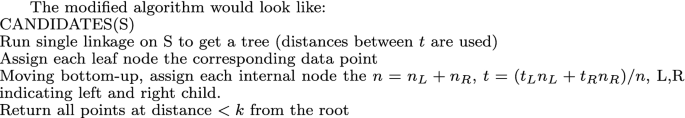

We would exclude clusters with several cluster members on the grounds of the fact that statistically speaking we want to be sure that the probability of an element occurring in the gap should be smaller than in a cluster, say p times. So if we have n elements in a cluster and none in the gap. then we should have \(\left( \frac{p}{p+1}\right) ^n \le 0.05\) for example. With p=10, we need a minimal cluster size of at least n=32.


References
Ackerman, M (2012) Towards theoretical foundations of clustering,. University of Waterloo, PhD Thesis.
Ackerman, M., Ben-David, S., & Loker, D. (2010) Characterization of linkage-based clustering. In COLT 2010 - The 23rd Conference on Learning Theory, Haifa, Israel , 27-29, 2010, (pp. 270–281).
Ackerman, M., Ben-David, S., & Loker, D. (2010) Towards property-based classification of clustering paradigms. In J.D. Lafferty, C.K.I. Williams, J. Shawe-Taylor, R.S. Zemel, and A. Culotta, editors, Advances in Neural Information Processing Systems 23, (pp 10–18). Curran Associates, Inc.,
Ackerman, M., Ben-David, S., Loker, D., & Sabato, S.(2103) Clustering oligarchies. In Proceedings of the Sixteenth International Conference on Artificial Intelligence and Statistics, AISTATS , Scottsdale, AZ, USA, April 29 - May 1, 2013, (pp. 66–74).
Ackerman, M., & Dasgupta, S. (2014) Incremental clustering: The case for extra clusters. In Advances in Neural Information Processing Systems 27: Annual Conference on Neural Information Processing Systems 2014, December 8-13 2014, Montreal, Quebec, Canada, (pp. 307–315) .
Ambroszkiewicz, S., & Koronacki, J. (2010) O pewnym wyniku orzekaja̧cym niemożność przeprowadzenia analizy skupień. krótki dowód z komentarzem. Decision Support Systems Conferernce, Zakopane, Poland, 2010, lecture, .
Arthur, D., & Vassilvitskii, S. (2007) \(k\)-means++: the advantages of careful seeding. In N. Bansal, K. Pruhs, and C. Stein, editors, Proc. of the Eighteenth Annual ACM-SIAM Symposium on Discrete Algorithms, SODA 2007, (pp. 1027–1035), New Orleans, Louisiana, USA, 7-9 Jan. SIAM.
Ben-David, S. (December 2005) Attempts to axiomatize clustering, 2005. NIPS Workshop,.
Ben-David, S., & Ackerman, M. (2009) Measures of clustering quality: A working set of axioms for clustering. In D. Koller, D. Schuurmans, Y. Bengio, and L. Bottou, editors, Advances in Neural Information Processing Systems 21, (pp 121–128). Curran Associates, Inc.,.
Blum, A. (2009) Thoughts on clustering . essay for the 2009 nips workshop "clustering: Science or art?"
Carlsson, G., & Mémoli, F. (2008) Persistent clustering and a theorem of j. kleinberg. arXiv preprint arXiv:0808.2241,.
Carlsson, G., & Mémoli, F. (2010). Characterization, stability and convergence of hierarchical clustering methods. Journal of Machine Learning Research, 11, 1425–1470.
Duda, R. O., Hart, P. E., & Stork, G. (2000). Pattern Classification (2nd ed.). New York: J. Wiley & Sons.
Hopcroft, J., & Kannan, R. (2012) Computer science theory for the information age, chapter 8.13.2. A Satisfiable Set of Axioms. page 272ff.
Kanungo, T., Mount, D. M., Netanyahu, N. S., Piatko, C. D., Silverman, R., & A. Y. Wu. A (2002) local search approximation algorithm for k-means clustering. In Proceedings of the 18th Annual Symposium on Computational Geometry, Barcelona, Spain, June 5-7, 2002, (pp. 10–18)
Kleinberg, J. (2002) An impossibility theorem for clustering. In Proc. NIPS 2002, pages 446–453,http://books.nips.cc/papers/files/nips15/LT17.pdf.
Klopotek, M., & Klopotek, R. (2021) Issues in clustering algorithm consistency in fixed dimensional spaces. some solutions for k-means. to appear in Journal of Intelligent Information Systems,.
Klopotek, M. A. (2019) A note on k-means probabilistic poverty. CoRR, abs/1910.00413,.
Klopotek, M. A. (2020). An aposteriorical clusterability criterion for k-means++ and simplicity of clustering. SN Computer Science, 1(2), 80.
Klopotek, M. A., & Klopotek, R. A. (2020) In-the-limit clustering axioms. In Artificial Intelligence and Soft Computing, volume 12416 of LNCS, (pp. 199–209). Springer,.
Klopotek, M. A., Wierzchon, S. T., & Klopotek, R. A. (2020) k-means cluster shape implications. In Artificial Intelligence Applications and Innovations, volume 583 of IFIP Advances in Information and Communication Technology, (pp. 107–118). Springer,.
Kłopotek, M.A. (1991) On the phenomenon of flattening ’flexible prediction’ concept hierarchy. In Fundamentals of Artificial Intelligence Research. International Workshop, volume 535 of LNAI, (pp. 99–111). Springer
Klopotek, R. A., & Klopotek, M. A. (2019) robabilistic k-richness of the k-means algorithms. In Machine Learning, Optimization, and Data Science, volume 11943 of LNCS, (pp. 259–271). Springer
Meilǎ, M. (2005) Comparing clusterings: An axiomatic view. In Proceedings of the 22Nd International Conference on Machine Learning, ICML ’05, pages 577–584, New York, NY, USA, ACM.
Ostrovsky, R., Rabani, Y., Schulman, L. J., & Swamy, C. (January 2013) The effectiveness of lloyd-type methods for the k-means problem. J. ACM, 59(6):28:1–28:22. 0.0000001 is epsilon so that epsilon square<target kmeans for k/target kmeans for k-1.
Song, M., & Rajasekaran, S. (2010). Fast algorithms for constant approximation k-means clustering. Transaction MLDM, 3(2), 67–79.
Steinbach, M., Karypis, G., & Kumar, V. (2000) A comparison of document clustering techniques. In Proceedings of KDD Workshop on Text Mining, Proceedings of the 6th International Confer1193 ence on Knowledge discovery and Data Mining, Boston,MA, (2000).
van Laarhoven, T., & Marchiori, E. (2014). Axioms for graph clustering quality functions. Journal of Machine Learning Research, 15, 193–215.
von Luxburg, U. (2009). Clustering stability: An overview. Foundations and Trends in Machine Learning, 2(3), 235–274.
von Luxburg, U., Williamson, R. C., & Guyon, I. (2011) Clustering: Science or art? initially, opinion paper for the NIPS Workshop "Clustering: Science or Art" in 2009,
Wright, W. E. (1973). A formalization of cluster analysis. Pattern Recognition, 5(3), 273–282.
Zadeh, R. B., & Ben-David, S. (2009) A uniqueness theorem for clustering. In Proceedings of the Twenty-Fifth Conference on Uncertainty in Artificial Intelligence, UAI ’09, (pp. 639–646), Arlington, Virginia, United States. AUAI Press.
Acknowledgements
The authors wish to thank to the Institute of Computer Science of Polish Academy of Sciences for promoting and financing this research. Research done by Robert A. Kłopotek was financed by research fellowship within Project ’Information technologies: research and their interdisciplinary applications’, agreement number UDA-POKL.04.01.01-00-051/10-00.
Funding
The research was funded by the Polish Ministry for Science – the Ministry finances the budget of the Institute of Computer Science of Polish Academy of Sciences [a purely research institution] and the Institute pays the regular salaries for the employees
Author information
Authors and Affiliations
Contributions
MA K – predominantly theoretical foundation RAK – predominantly simulation experiments verifying the theorem, programs to generate drawings, English. We show that Kleinberg's proof of non-consistency of k-means is not appli-cable in fixed dimensional space. k-means is consistent in 1d (see Section3.1), For higher dimensions non-consistency must be proven differentlythan Kleinberg did (Section 3.2) [theory predominantly by R.A.Kłopotek] • We show in Section 4.2 that consistency property alone leads to contra-dictions in Rm. [theory predominantly by R.A.Kłopotek]. We propose a reformulation of the Kleinberg's axioms in accordance withthe intuitions and demonstrate that under this reformulation the axiomsstop to be contradictory (Section 6). In particular we introduce the notionof centric-consistency (Section 5)We provide a clustering function that _tsthe axioms of near-richness, scale-invariance and centric-consistency. [theory predominantly by M.A.Kłopotek]. We show that k-means is centric-consistent (Section 5). Hence a real-world algorithms like k-means conforms to an axiomatic system consisting of: centric-consistency, scale-invariance and k-richness(Section 5). [theory predominantly by M.A.Kłopotek]. We demonstrate in Section 6 that a natural constraint imposed onto Klein-berg's consistency leads directly to the requirement of linear scaling, so that the centric consistency can be considered LESS restrictive than his. [theory predominantly by MAK] We demonstrate there exists an algorithm (from the k-means family) that matches the axioms of constrained consistency, richness and invariance. [theory predominantly by R.A.Kłopotek] As the centric consistency imitates only the consistency inside a cluster, we introduce the notion of motion consistency, to approximate the consistency property outside a cluster and show that k-means is motion-consistent (Section 7) only if a gap between clusters is imposed. [theory predominantly by MAK] We show that appropriately designed gaps induce local minima (Section 8) for k-means and formulate conditions under which the gap leads to a global minimum for k-means (Section 9). [theory predominantly by MAK] We propose an alternative approach to reconcile Kleinberg's axioms with k-means by either relaxing centric consistency to inner cluster consistency or k-richness to an approximation of richness (Sections 8 and 9) [theory predominantly by MAK]
Corresponding author
Ethics declarations
Conflict of interest
Not applicable
Consent to participate
Mieczysław A. Kłopotek agrees to participate. Robert A. Kłopotek agrees to participate.
Consent for publication
Mieczysław A. Kłopotek agrees that his individual’s data and image are published Robert A. Kłopotek agrees that his individual’s data and image are published
Ethics approval
Not applicable
Additional information
Editor: Xiaoli Fern.
Publisher's Note
Springer Nature remains neutral with regard to jurisdictional claims in published maps and institutional affiliations.
Rights and permissions
Open Access This article is licensed under a Creative Commons Attribution 4.0 International License, which permits use, sharing, adaptation, distribution and reproduction in any medium or format, as long as you give appropriate credit to the original author(s) and the source, provide a link to the Creative Commons licence, and indicate if changes were made. The images or other third party material in this article are included in the article's Creative Commons licence, unless indicated otherwise in a credit line to the material. If material is not included in the article's Creative Commons licence and your intended use is not permitted by statutory regulation or exceeds the permitted use, you will need to obtain permission directly from the copyright holder. To view a copy of this licence, visit http://creativecommons.org/licenses/by/4.0/.
About this article

Cite this article
Kłopotek, M.A., Kłopotek, R.A. On the Discrepancy between Kleinberg’s Clustering Axioms and k-Means Clustering Algorithm Behavior. Mach Learn 112, 2501–2553 (2023). https://doi.org/10.1007/s10994-023-06308-x
Received:
Revised:
Accepted:
Published:
Issue Date:
DOI: https://doi.org/10.1007/s10994-023-06308-x