Using the Bifocal Modeling Framework to Resolve “Discrepant Events” Between Physical Experiments and Virtual Models in Biology

Abstract

In this paper, we investigate an approach to supporting students’ learning in science through a combination of physical experimentation and virtual modeling. We present a study that utilizes a scientific inquiry framework, which we call “bifocal modeling,” to link student-designed experiments and computer models in real time. In this study, a group of high school students designed computer models of bacterial growth with reference to a simultaneous physical experiment they were conducting, and were able to validate the correctness of their model against the results of their experiment. Our findings suggest that as the students compared their virtual models with physical experiments, they encountered “discrepant events” that contradicted their existing conceptions and elicited a state of cognitive disequilibrium. This experience of conflict encouraged students to further examine their ideas and to seek more accurate explanations of the observed natural phenomena, improving the design of their computer models.

Introduction

The nature and role of school science laboratories have been subject to widespread controversy in the research community (NRC 1996), especially regarding the benefits of physical, virtual, and combined laboratories (Olympiou and Zacharia 2012; Triona and Klahr 2003; Zacharia 2007). The popularity of simulation environments such as PhET (Perkins et al. 2006) has led policy-makers and scholars to question the real value of physical laboratories—especially in the face of the associated costs and logistics. A wave of research studies within the past 10 years has explored: (a) What are the advantages of physical laboratories relative to virtual laboratories and manipulatives, (b) whether the latter can replace the former (Triona and Klahr 2003), and (c) in what ways virtual models can simulate complex phenomena and permit student experimentation in domains that might otherwise be costly, impractical, or dangerous (Finkelstein et al. 2005; Jaakkola and Nurmi 2008; Jaakkola et al. 2011; Klahr et al. 2007; Perkins et al. 2006; Resnick and Wilensky 1998).

The literature comparing hands-on or physical models (PM) with virtual models (VM) for science learning has sought to establish rules for choosing one modality over the other or for ordering them as distinct phases in a sequential process (de Jong et al. 2013). Zacharia and Anderson (2003) found that combining physical and virtual models increased teachers’ learning of content knowledge in physics. Zacharia and Constantinou (2008) recreated this result with undergraduate physics students by first employing a physical model rather than a virtual one, and Jaakkola and Nurmi (2008) obtained similar results for elementary school students. Most of these early studies pointed to the advantage of virtual over physical laboratories, but soon researchers found that the combination of the physical and virtual laboratories led to greater conceptual understandings than did either type singly. For example, Liu (2006) compared groups of female high school students utilizing computer simulations and/or hands-on laboratory activities in chemistry. Controlling for time-on-task, the combination of both PM and VM was more effective than either option alone. But interesting interactions between content learning and epistemology were observed for this composite approach: There was a correlation between students’ understanding of the chemistry content and a belief that the chemistry model demonstrated was an exact replica of reality. In other words, students who understood the content better were not necessarily more epistemologically sophisticated. This finding is a preliminary indication of the importance of directly addressing epistemological issues in both laboratory- and model-based inquiry environments, either in virtual, physical, or combined models.

The literature further suggests that while multiple representations can help students understand underlying scientific concepts, they can also be overwhelming to new learners who may not know what are appropriate elements of each representation on which to focus (Kirschner et al. 2006). One approach to helping new learners make sense of these multiple representations is to link them explicitly, so that changes in one modality will directly affect the other. Van der Meij and de Jong (2006) investigated this question in a virtual physics learning environment, employing multiple graphical representations to convey the relationships between variables in a mechanical system. In one experimental setup, the representations were dynamically linked so that each responded to changes in the other, and they were “integrated” through their close visual proximity to each other. In a second condition, the variables were integrated but unlinked, and, in a third, they were both unlinked and unintegrated. The authors found that students who learned the most were best able to transfer their new knowledge to new problems, and that these same students reported the least difficulty with the version that was both linked and integrated—a finding that expands upon the design principle of “multiple representations” (Blake and Scanlon 2007). However, intergroup differences emerged only when more challenging problems were presented to the students. Although all groups’ performances were approximately equal for the easier questions, the results suggest that for more difficult problems involving the use of many sources of information, scaffolding becomes increasingly important. The authors explain this finding in terms of scaffolding’s ability to reduce the working memory load the students require for tracking multiple representations carefully enough to identify their relationships.

Together, these findings suggest that combining and linking computational tools and physical laboratories has considerable potential for classroom science learning. While the potential of this combination of virtual and physical models as a tool for science learning has been documented over a wide range of ages and domains, the findings also point to a need for better design principles and theoretical frameworks to determine how this potential may be leveraged to address the cognitive, pedagogical, and epistemological issues at play in the science classroom.

In particular, two areas in this realm have not been researched sufficiently. First, the literature has focused almost entirely on predesigned physical and computer models or laboratories. Predesigned models can provide scaffolding and make students aware of relevant information about a problem, but they fail to provide students opportunities to evaluate the assumptions and limitations of the models themselves (Papert 1980). The practices of creating and critically evaluating models constitute an important part of scientific practice and have been valued increasingly as educational goals (Blikstein and Wilensky 2006; Blikstein 2010; Gire et al. 2010). Second, the literature has not adequately explored the potential for deeper support for students’ explicit comparisons between physical and virtual models. Most such work focuses either on the comparison of physical and virtual laboratories or on their sequencing, but not on the mutual synergies they create when connected in real time. When these synergies are explored, the virtual laboratories employed are often transpositions of physical laboratories to a virtual environment: Beakers, test tubes, and chemicals are simply made virtual in a computer-based environment, and students use these representations to conduct experiments. For example, Smith et al. (2010) noted that scaffolds in virtual models or direct data sharing between virtual and physical models could help students recognize the similarities and differences between the model and reality. But when scientists use models and simulations together with real-world data, they are looking for synergies rather than replacements—they use virtual and physical models to bring to the table different kinds of information, questions, and insights.

The Bifocal Modeling Framework

The bifocal modeling framework (BMF) (Blikstein 2010, 2012, 2014) is an approach to inquiry-driven science learning that involves the investigation of natural phenomena through the real-time coordination of physical experimentation and virtual modeling. The approach challenges students to design and compare physical experimentation coordinated with the construction of virtual models with the goal of identifying the respective advantages, differences, and limitations, of these discrete modalities for the study of nature. In these activities, students explore, through physical experiments, scientific phenomena such as heat diffusion, the properties of gases, and wave propagation; design virtual models; and, in real time through iterative comparisons, connect their experiments’ empirical data sets with their models. During the physical phase of the process, students first design and develop a physical experiment. Next, as they conduct the experiment, they utilize embedded sensors or time-lapse cameras to collect data. Concurrent with their physical experimentation, the students design and develop a virtual model for the same phenomenon and compare the behavior of their virtual model with observations from their physical experiment (Fig. 1). Finally, when students identify discrepancies, they have opportunities to redesign their models and reiterate the process.

Fig. 1

Examples of bifocal models: gas laws (left) and Newton’s cradle (right)

Depending on the nature of the phenomenon studied in a bifocal activity, students can utilize various programming languages to implement their virtual models [NetLogo (Wilensky 1999), Scratch, etc.]. The students’ goal is to build a model whose behavior matches or imitates the physical data they collect. Through the comparison of the virtual model’s behavior with their experimental data, the students are able to discover discrepancies between the results of the different modalities. Piaget (1985) argued that to foster conceptual change, students must be confronted with “discrepant events” that contradict their conceptions and invoke a “dis-equilibration or cognitive conflict.” Following the forms of equilibration in Piaget’s theory, researchers (Hewson and Hewson 1984) identified two distinct types of cognitive conflicts: the conflict between the internal and external worlds of a student’s conceptions and experiences, and the purely conceptual conflict between two different cognitive structures related to the same phenomenon.

Given that the BMF may include many different tools and techniques, there are multiple possibilities for classroom implementation of each modality. To structure our studies, we divided the physical and the virtual assignments into a sequence of shorter activities. Each modality includes three main assignments: design (which includes planning), construct, and interact (Fig. 2):

Fig. 2

General structure of a bifocal modeling activity (Blikstein et al. 2012)

• 1. Design Students select a research question, plan their observation, generate hypotheses, and design experiments and virtual models that will potentially confirm them. In designing the virtual model, students define variables and conceptualize micro-rules or equations to describe the phenomenon.

• 2. Construct Students structure both their physical experiment and virtual model.

• 3. Interact Students interact with their experiments through direct observation or the use of embedded sensors/cameras; they interact with their computer models by changing parameters; and they record data.

The empirical phenomenon of bacterial growth in a Petri dish exposes students to a complex system with many variables. We chose bacterial growth because of the simple cellular structure of bacteria, their rapid reproduction, and the complex ecological dynamics of the phenomenon. Our goal was for students to recognize the distinctive patterns of each of the four stages of the bacterial growth curve (Fig. 3), to understand the variables underlying these patterns, and to explain the mechanisms of each. The four stages are explained below.

Fig. 3

Bacterial growth curve over time (cell population given in log scale)

• A. Lag phase Bacteria population remains temporarily unchanged; during this phase, the bacteria adjust to their new environment, repressing or inducing enzyme synthesis, and initiating chromosome replication.

• B. Log phase Bacteria growth proceeds by “binary fission,” a process by which individual bacteria divides into pairs. Exponential growth cannot continue indefinitely because the medium is soon depleted of nutrients, which are replaced by waste products.

• C. Stationary phase The population remains constant because the rate of bacterial growth is equivalent to the death rate.

• D. Death phase In this final stage, the bacteria have exhausted their nutrients, lose their ability to divide, and die off. As in the rapid growth phase, the decay pattern characterizing the death phase is exponential (1)

In this study, we will describe and evaluate our attempt to utilize the BMF to teach 9th grade students the behavior of biological systems in general and, specifically, the bacterial growth dynamic.

Methods and Research Setting

Participants

The study was conducted with 13 students (4 females and 9 males) and lasted for a total of 3 days (about 15 h) in a university laboratory setting. Students came from a 70 % minority high school located in a predominantly Latino urban community and had volunteered for the 4-week, 30-h/week digital fabrication workshop at a research university. This workshop took place during the school’s intersession, during which all students were required to enroll in a month-long extracurricular course or internship outside of school. The selection of students was governed by a complex allocation system developed by the school, which resulted in a sample that was approximately representative of the school’s diversity.

Data Sources

All students were videotaped during all activities, their computer usage was logged with screen-capture software, the researchers conducted informal interviews and kept field notes, and all students’ notes and sketches were saved. Following the transcription of the entire 15 h of video recordings, all data were analyzed by the researchers. Episodes explicitly showing moments of comparisons between the virtual model and the physical experimentation were selected by the research team as the focus of this study. To reveal the discrepancies in these episodes, the researchers analyzed the content and the context of the situations in the video recordings in order to identify iterative moments of comparison.

Instructional Sequence

The 15 h of work was divided into four main activities (Fig. 4):

Fig. 4

Four activities of the study

• 1. Introduction and physical experimentation After the students were given an introduction to bacterial growth, they were tasked to grow real bacteria. They prepared a Petri dish with agar and collected a bacteria sample from an object likely to be contaminated (e.g., a door knob, keyboard, toilet). It was predicted that students would collect different species of bacteria as well as fungal species and not pure bacterial culture. Fortunately, the morphology of bacteria colonies is different than fungal colonies, so researchers  could show students how to discriminate between colonies easily. The Petri dishes were incubated at room temperature. The students were also provided a time-lapse camera to capture images of the Petri dishes at 30-min intervals over 7 days. The images were automatically compiled into a video. In response to time restrictions, the workshop facilitators also showed the students a video of a bacterial growth experiment conducted previously by the research team in the same laboratory with the same toolkit.

• 2. Web inquiry and presentation Students were grouped into pairs and asked to make a list of questions about bacteria and bacterial growth. They were asked to conduct Web research to answer these questions, and they presented their findings to the entire class in short slideshows.

• 3. Collaborative “whiteboard programming” Students were then divided into three groups, each of which was provided a dedicated facilitator from the research team. Each group was asked to determine the rules that govern bacterial growth. First, students listed all variables they thought would affect bacterial growth. Next, the facilitator proposed the iterative construction of a block-based “computer program” on the whiteboard (Fig. 5), in which the students were to generate the main stages of bacterial growth and to account for the development of each stage and the interaction of the variables. After 3 h of “whiteboard modeling,” the student groups were split and reformed so that each individual was able to share their ideas with two members from other group during a 45 min discussion panel. After receiving feedback on their initial ideas from members of the other groups, the original groups were reconvened and began programming their virtual experiment in NetLogo.

  Fig. 5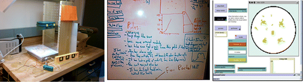

  

  Experiment with time-lapse camera, “whiteboard modeling,” and virtual model

• 4. Programming and comparing experiments and virtual models In the fourth and final phase, the facilitator sat facing the group in front of a large television used for displaying code; In this phase the facilitator’s role was to “translate” the ideas of the students into NetLogo code. These final 3 h of student engagement in our study were dedicated to coding the students’ virtual model and comparing the coding results with the data collected from the experiment in the Petri dish. Students discussed the results, developed hypotheses for approaches to the validation of both models, and made changes to the virtual model in order to bring it into closer accord with the real bacterial growth observed empirically in the Petri dish.

In summary, students created a whiteboard model and translated their whiteboard rules into a model’s specifications. Next, they “ran” the model to envision how bacteria would multiply according to the model and compared the modeled results both with the empirical observations of Petri dish growth patterns and with a growth curve they were given by the researchers. Finally, the students refined the virtual model by adding rules and variables to address the perceived differences between the model and the experiment. In Fig. 6, we present a diagram of our hypothesized pedagogical model’s chronological sequence of the typical phases of the students’ design process. This group repeated the above design process a total of four times during the 1.5 h of the final session (activity four).

Fig. 6

Diagram of the iterative design process separated into steps for the purposes of this analysis

Data and Discussion

Since the main focus of this paper is the analysis of discrepant events in the modeling process, we will not focus on the programming of the models, but on their conceptualization prior to programming. The data are presented as a representative sample of the model comparison moments and the discrepant events that students encountered during the activity. In what follows, we focus on two groups of students and present five episodes that demonstrate students’ encounters with the discrepant events. To explain and analyze the episodes, first we introduce the context for the episode, and then the students design process, which for the purposes of this analysis, we broke down into the following five stages: (a) computer model, (b) physical experiment, (c) discrepancy, (d) discourse, and (e) solution. Finally, we discuss the results from the five sample episodes.

Episode # 1: How Do Bacteria Move?

In this first episode, students faced a specific conflict while comparing the virtual design results to the actual colonies in the Petri dish. They discovered that in the physical Petri dish, bacteria do not confine their reproduction to a single location; rather, they reproduce and migrate. This observation of the experimental results and comparison to the model suggested the idea that bacteria do not grow on top of each other; rather, they spread out. The following is an account of an instance of the students’ design process divided into the five steps described above:

• a. Computer model

The first step of the design process involved planning the virtual model on the whiteboard. The students decided to include agents such as bacteria and food, as well as a rule regarding reproduction. “Running” this model resulted in the exponential growth of individual bacteria. Each new time step resulted in an increased bacterial population that was confined to its original location on the virtual Petri dish.

• b. Physical experiment

While observing the physical Petri dish, students noticed that bacteria had a specific and unique growth pattern—they do not grow on top of each other; rather, they spread throughout the dish.

• c. Discrepancy

In their comparison, the students observed a mismatch; they saw that physical bacteria colonies in the Petri dish did not resemble the virtual colonies of their model. In the experiment, bacteria reproduced and spread out, forming differently shaped colonies, but in the virtual model, they grew on top of each other, forming a localized concentration of bacteria.

• d. Discourse

At this point, students began to generate questions about the phenomenon and sought answers for these questions in their groups. They asked questions about: the mechanisms for the development of the bacteria’s unique growth patterns, the mechanisms for and causes of bacterial motion, and whether or not bacterial motion was random. The following is an excerpt from their discussion:

Student 1::

Do we know if they move around randomly?

Student 2::

How else would they move around?

Student 4::

Maybe in specific ways that we could understand…

Student 1::

I guess, like, where they scooted, go toward the food, but it could just do that…

Student 2::

What makes you think this is fine or not? How do you know?

Student 2::

I think it doesn’t really matter how they move

Instructor::

Doesn’t really matter for what?

Student 2::

What do you mean?

Student 1::

Like, how do you know it doesn’t really matter, you know?

Student 2::

Well, I mean, they’ll eventually find food by moving randomly

The observation of the physical Petri dish and the ensuing realization of the model mismatch triggered a discussion of possible mechanisms for bacterial motion. They began to seek possible ideas to debug the model in order to make it correspond to the actual Petri dish. The discussion progressed to a conversation about physical micro-mechanisms that might explain the phenomenon: For instance, one student suggested that the bacteria might have whip-like flagella at their anterior ends, while another offered that the bacteria might move randomly.

• e. Solution

After the discussion, students decided to add a new rule to their designed virtual model, which helped simulate the random movement of the bacteria in the virtual Petri dish and resulted in colonies that spread across the virtual dish in a pattern resembling that of the physical experiment (Fig. 7).

Fig. 7

A whiteboard model resulted in an increased bacterial population confined to an original location, reproduced on top of each other (right). A physical experiment in a Petri dish with bacteria colonies spread across the dish in specific patterns (left)

Episode # 2: Are There Many Types of Bacteria in a Single Petri dish?

In this second episode, the students discovered that bacteria colonies in the physical Petri dish are not uniform in appearance: Rather, they differ in shape, texture, and color. This observation and comparison of the experimental and modeling results suggested the idea that bacteria in the Petri dish do not originate from a single bacterium: Rather, they are reproductions of different species of bacteria.

• a. Computer model

During this stage, students were still in the process of designing their virtual model on the whiteboard. They had already added two types of agents to the model, bacteria and food, and they had also added rules regarding reproduction and movement. The entailments of this planned model resulted in an exponential growth of bacteria that spread across the virtual dish producing colonies in a pattern resembling the one in the physical dish. Each additional time step resulted in an increased population of only one type of bacterium.

• b. Physical experiment

While observing the physical Petri dish, students noticed that bacteria colonies appear to have specific and unique patterns. The Petri dish included several types of bacterial colonies that differed in appearance, with unique variations of color, shape, and texture. These differing types of colonies also spread throughout the dish in their own characteristic patterns, and the students surmised that these differences corresponded to different species of “parent” bacteria.

• c. Discrepancy

The Petri dish contained several types of bacteria colonies, which produced a very rich spread with much variation among colonies in terms of shape, texture, size, and color. However, the virtual model produced only a single type of bacteria, and the colonies resembled each other. It seems that the model produced too much uniformity, and that the increased complexity of the actual phenomenon likely resulted from the speciation of the bacteria.

• d. Discourse

While comparing and validating their design, students asked questions including: How many types of colonies are in one Petri dish? What is the origin of the colonies? How many and what are the “seeds” of the colonies for the reproduction of bacteria? The following is an excerpt from the group discussion, which led the students to revisit their computer models:

Student 1::

I saw that there are different colors of bacteria on our Petri dish

Student 2::

They…the bacteria also look different, not similar shape and color. In the (computer) model it is the exact same bacteria. How can we change it?

Student 3::

In the real experiment, I notice that there are different kinds of bacteria. Maybe it’s because they reproduced from a different source

Student 2::

We need to make different types of bacteria (in our model)

• e. Solution

At this stage, the students sought to solve the problem by introducing multiple types of bacteria into their model. Students then added a new rule that created a variety of initial pools of differently colored “seed” bacteria, each representing a distinct species. This improved simulation resulted in several types of bacteria colonies, which differed in color and spread across the virtual dish, resembling more closely what was observed for the natural phenomenon.

Episode # 3: How do Bacteria Split While Reproducing?

In the initial stage of the design process, the students’ attempt to validate their models led to a crucial question about reproduction. They decided to make the bacteria reproduce, but they were not certain about the process’ mechanism. They sought to learn more about it through an examination of the physical Petri dish, but while they could clearly see colonies, they were not able to observe the behavior or reproduction of individual bacteria on the microscopic level. Since students were required to design an agent-based computer model on their own, they decided to consider the behavior of a single bacterium. The following is the design process divided into five steps:

• a. Computer model

Modeled bacteria moved randomly and reproduced. Each individual bacterium gave birth to two new individuals; the “parent” bacterium produces two offspring distinct from itself for a total of three. Running the virtual model resulted in an increased bacterial population.

• b. Physical experiment

While trying to correlate their design and model to the physical experiment, students realized that it was impossible to see the way bacteria divide with the unaided eye and sought answers elsewhere. They started to question the way bacteria reproduce and searched the Internet for answers.

• c. Discrepancy

During their web research, the students found a video of the reproduction of actual bacteria under the microscope and discovered that bacteria reproduce by binary fission, resulting in two new bacteria, but no parent. The actual reproduction process contradicted their design.

• d. Discourse

Even though the Petri dish experiment did not permit the students to observe the microscopic details of bacterial reproduction, it did lead them to discuss the topic in their groups and to seek answers elsewhere. Seeking to explain the phenomenon, the students asked questions such as: Does one bacterium “give birth” to two different “baby” bacteria? Does that mean that a “parent” bacterium produces two offspring for a total of three? Or does each individual bacterium become two new individuals? The following is an excerpt from the group discussion:

Instructor::

What does it mean to reproduce here? Should they just, like, one turn into two?

Student 2::

Yeah

Instructor::

Split? Okay

Student 4::

Wait. Does—one turns into two, you said?

Student 1::

Mm-hmm

Student 4::

Or would it be one makes two or no?

Instructor::

Ah, so it’s like the difference between splitting in half and giving birth to twins. Which one do bacteria actually do?

Student 4::

They split

Student 1::

Twins

Student 4::

They just split in half

Instructor::

And here split, and you’re twins. Okay. Can we … maybe we can look it up real quick

• e. Solution

Eventually, the students decided to go with the “split” rule and added a new “reproduce” rule to their virtual model. This rule stated that “every 20 ticks the bacteria would split into two,” which resulted in the exponential growth of the bacteria. Below is a photograph of the whiteboard used in the students’ design process (Fig. 8).

Fig. 8

Whiteboard model with the new “reproduction” rule for bacteria: “every 20 ticks split”

Episode # 4: Do Bacteria Have an Infinite Life Cycle?

While examining and running their virtual model, the students discovered that the bacteria would not stop reproducing and would live indefinitely. However, these virtual results did not correspond to what was actually observed in the physical experiment; therefore, they began questioning bacterial death as a conclusion to colony propagation. Their next step was to seek a mechanism that would induce bacterial death through the manipulation of food resources.

• a. Computer model

In their computer model, the students made their virtual bacteria move randomly and reproduce every 20 ticks. The bacteria reproduced without interruption, and their population increased until they completely covered the virtual Petri dish and continued to increase indefinitely.

• b. Real experiment

Observation of the actual Petri dish experiment led the students to realize that the size increase of the empirical bacteria colonies was not unlimited. After several days, the individual colonies ceased to expand and remained the same size. Additionally, the students became aware of the bacterial growth curve, which includes a death phase. They realized that, eventually, the bacteria in the physical experiment begin to die off and that bacteria do not live indefinitely.

• c. Discrepancy

In the physical experiment, the students realized that bacterial life is not without limits, and that the colonies produced boundaries when they ceased expansion after a relatively limited term. Yet, in the virtual model, the bacteria reproduced every 20 ticks indefinitely, and the students realized that there was a fundamental difference between the growth patterns of the empirical and virtual experiments.

• d. Discourse

In this phase, students discussed environmental conditions that might prevent the unlimited reproduction of the bacteria. After considering specific environmental variables (food, waste, water, etc.), the students focused on the effect of the availability of food on bacterial population and life cycle. In the following excerpt of students discussion of this subject, the students had been asked to figure out how to “translate” the rule of limited food resources into NetLogo. They added a new type of agent to the model, “bacteria’s food,” and programmed it so that, once the food was exhausted, the bacteria would cease reproducing and die off. The following is an excerpt from the group discussion:

Student 2::

Look at the death

Student 1::

Death?

Student 4::

What should happen is that they run out of food

Student 3::

Okay. How should we—how should we do that? Can we make some—write some imaginary code for that?

Student 2::

Made some of the (food pieces) disappear

Instructor::

So can you give me more? Imagine that I’m, like, really like a dumb computer. You need to tell me the steps I need to take. Is it, like, when all that is gone, then they all die?

Student 1::

The bacteria

Student 4::

They slowly die. They still reproduce, but they slowly die

Student 1::

Okay. And when is it, like, every tick or…?

Student 2::

Every ten

Student 3::

If all (food pieces)—all 100 (food pieces) are gone, then bacteria die

Instructor::

If all food is gone, then all bacteria die. Okay. Let’s run the model in our heads and think about how we’re going to do it. So all the food is gone…eventually when they run out of food, boom, they die. They all die. That’s the code we have right now

• e. Solution

Students added the “food” agent to their design. The corresponding rule was that when food is exhausted, and no new food resources are available, the bacteria die. Therefore, in the revised design, thus, bacteria no longer had an unlimited life span.

Episode # 5: When do Bacteria Start Reproducing?

After “running” the virtual model from episode # 4, a student observed a further mismatch: The simulated growth curve exhibited an exponential increase from the outset, which she noted was incorrect because the physical growth curve initially exhibited a flat “lag phase.” After a long discussion, group members attempted to explain the lag phase of the bacterial growth, which commenced with the incubation of the Petri dish.

• a. Computer model

In their model, students made their virtual bacteria begin reproducing as soon as they were introduced into the Petri dish.

• b. Physical experiment

After comparing their model’s results with the curve derived from observations of the physical experiment, the students became aware of the lag phase that occurs before bacterial reproduction becomes apparent. They discovered that it took about 5 days before they could detect a visible colony on their Petri dish. This discovery led them to realize that specific conditions must be met for bacterial reproduction to become visible.

• c. Discrepancy

It took time for students to realize that there is a “lag phase” at the outset of the bacterial growth process. In the physical Petri dish, 5 days elapsed before the students observed visible alterations of the agar medium and colony growth. However, in their initial model, bacteria grew and reproduced immediately. After comparing their computer model with the results of both the experiment and the bacterial growth curve, the students realized that the initial stage of the physical experiment evinced no visible change in bacteria population. This conflict engaged them in rethinking the phenomena they were attempting to model, and led them to revise their model according to their observations of the physical experiment.

• d. Discourse

In order to clarify this discrepancy and to achieve a better correlation with their observed results, the students needed to find, for inclusion in their model, an explanation for the initial “lag” phase of bacterial growth. Here is an excerpt of the group discussion:

Instructor::

What about the, I am asking again because I’m really trying to make a point here. Remember, they didn’t start like this in the graph? They didn’t just reproduce? … and we did it like that and we had this phase which they don’t change, … yeah. What happen there?

Student 4::

The lag?

Student 3::

What is happening? Yeah, what is happening to them, the bacteria in real bacteria dish?

Student 2::

Because it takes a while for it to form and like reproduce. As soon as they get the hang of it, they’re like, yeah, to make more

Student 3::

So they get used to their… like they get used to their environment

Student 4::

Their place

Instructor::

So how can we do it in program? What do we need to add there?

Student 3::

Maybe like a spurt where they’re having a bunch of babies, and they kind of stop having babies, then they start having babies again. Have it slowly…

Student 4::

Slowly, so they won’t start at the beginning?

Student 2::

Yeah then they start, and then they don’t, and then they start

Student 1::

Are you trying to make it like this?

Instructor::

How can we turn this idea of the lag phase into a code?

Student 2::

I guess we can use a wait, about like twenty ticks—oh that’s a lot, a lot of wait, like ten ticks, to get used to the environment, so they can just say wait… 10 days before starting to reproduce?

Instructor::

Good idea

• e. Solution

In the process of generating a virtual model that better emulated the natural phenomena, the students added behavior parameters and behavior sequences in ways that either related explicitly to real-world behaviors or included real-world constraints. In this episode, the students added rules so that their modeled bacteria would only reproduce after they got “used to” their environment. In this case, the students’ implementation of their designed model included the following manipulations of the food variable. If the model’s food value is greater than ten (one food piece is added at each time step throughout the model), the bacteria reproduce; if this value is less than ten, the bacteria first enter a lag phase and wait to reproduce (Fig. 9).

Fig. 9

Bacterial growth curve as it is in the model (right) without the lag phase and with the lag phase (left)

The table summarizes the sample episodes that demonstrate this iterative process by one of the groups. Notice the learning process occurs each time after the mismatch is revealed. Here we divided learning process into three steps: (1) Students ask an insightful question, (2) They rethink and understand the scientific concept, and (3) They revise the model, so it will explain the phenomenon (Table 1).

Table 1 Summary of the episodes

Discussion

In this paper, we have described an iterative process that students have gone through while designing a scientific model of bacteria growth. Their initial assignment was to conduct a physical experiment using a Petri dish, after which they were asked to design a model to explain the natural phenomenon observed in the experiment. As it is apparent in the preceding accounts, the process of model design was iteratively scaffolded in five steps:

• 1. Designing an initial computer model

• 2. Comparing that model’s results with those of the physical experiment

• 3. Detecting a discrepancy

• 4. Discussing the underlying reason for that discrepancy

• 5. Resolving the discrepancy

As additional discrepancies become evident, the process is repeated until the best match for the natural phenomenon is achieved. Students first generated a very simple model of bacterial growth and compared its output to their observations of the physical experiment. During this comparison, they encountered mismatches between the modeled outcome and the behavior of the actual bacteria. Next, the students considered the empirical mechanisms underlying these discrepancies and refined their computer model accordingly through the addition of new agents and rules. Our data reveal two types of learning patterns involved in the students’ engagement in this iterative design process: (a) navigation between the micro- and the macro-levels of the phenomenon and (b) the “translation” of an elaborate phenomenon into simple, micro-level rules:

• a. Navigation between the macro- and micro-levels of the phenomenon This pattern was characterized by the way students navigated between the macro-level behavior of bacteria populations visible as colonies in the Petri dish and the micro-level behaviors of individual bacteria cells. Our data indicate that although the students were not able to examine the behavior of individual bacteria during their observations of the physical experiment (i.e., students did not have access to microscopes or similar equipment), they could see a trend for the collective behavior of the bacteria at the colony level. Since students were required to design an agent-based computer model, while comparing it to their physical data results, they were led to a shift from consideration of the overall behavior of colonies to the behavior of single bacteria. For example, in episode 1, the students identified that empirically, bacteria colonies migrated randomly throughout the Petri dish, while the modeled bacteria colonies grew on top of each other in a single location. The iteration of their observations at the colony level in the Petri dish to their use of these observations to revise and correct their computer model required that the students understand the system at another level. Thus, to understand the behavior of the colony, the students needed first to understand and explain mechanisms that occurred at the micro-level in terms of behaviors of the individual bacteria. The issue of levels thinking has been extensively addressed in the literature (Wilensky and Resnick 1999; Wilensky and Reisman 2006; Levy and Wilensky 2009; Levy and Wilensky 2008; Blikstein and Wilensky 2007), and scholars have shown the benefits of having students transition between micro- and macro-levels of description of scientific phenomena. From our data, it seems that the bifocal framework afforded a new type of interaction: Students employed the real experiment as their macro-level representation “anchor,” while keeping the computational algorithm as their micro-level anchor. We argue that this recursive process not only enriched students’ inquiry process, but it provided a new type of epistemic game (Collins and Ferguson 1993) through which students could accelerate and deepen their sense about bacteria growth.

• b. Translation of a complex physical phenomenon into simple, micro-level rules As a result of the process described in (a), students translated the complex system behavior of the physical experiment into simple rules, which are implementable within a computational model. In episode 4, for instance, by going through the bifocal epistemic game, students were able to conclude that the bacteria colonies stopped expanding and remained the same size. Additionally, they became aware of the bacterial growth curve, which includes both steady growth and death phases. To simplify the complex system of the bacterial life cycle, the students focused on a single variable: the effect of the availability of food resources on bacterial population. In this specific episode, they added a new type of agent to their model, “bacteria’s food,” as well as a new rule, which established that the exhaustion of the food supply would lead to the cessation of bacterial reproduction and, subsequently, death and colony decline. Thus, the process of examining the bacterial life cycle, the realization that the life of bacteria is not unlimited, and the translation of the empirically observed behaviors into modeled rules constituted a key learning outcome for the students who participated in the bifocal modeling activity.

In both of the above learning patterns, students confronted discrepancies that motivated them to reach beyond physical experimentation and begin a process of inquiry that included questions, group discussion, and exploration to seek an explanation of the discrepancy. For example, in episode 3, the students lacked the benefit of microscopy and were unable to observe the bacterial reproduction process at the cellular level. However, comparison of their empirical observations and their virtual model inspired them to ask questions and conduct online research, which, in turn, lead to the discovery of video revealing the process under a microscope. In this case, students were provoked by the process of comparisons and their subsequent discovery of the mismatch between their model and the physical experiment to extend their inquiry process beyond the scope of the experimentation. During their model design, the students repeatedly compared and validated that model with reference to the physical experiment they were conducting. This comparison and the discrepancies it revealed encouraged students to further explore the bacterial growth phenomenon on different levels. The students then sought to expand their knowledge of bacteria growth by providing mechanisms for their computational model and translating complex empirical behaviors into modeled rules. The recursive, iterative process of model design encouraged students to experience a process utilized by scientists in various fields: the recursive refinement of a scientific model through repeated observations of scientific phenomena and the employment of those observations to correct and validate models.

Unfortunately, authentic implementations of this process of iterative comparison and recursive refinement occur in only a minority of science lectures and laboratories in high school. Because of the sequential character of typical class, the laboratory experiment is often too far removed from model design or equation exploration to provide meaningful feedback to the process of discovery. Consequently, such laboratories serve merely to verify previously learned content. This approach denies students the opportunity to deepen their understanding of scientific phenomena through comparison of the emerging results of concurrent physical experimentation with a model, and the opportunity to engage in a scientific modeling process. We believe that the implementation of a framework that integrates empirical research and scientific modeling offers students the opportunity to experience and engage in authentic scientific inquiry. In addition it offers a conceptual understanding through repeated comparisons of the virtual model and the observations of physical experimentation.

Conclusion

The rise of computer models and simulations in the research of highly complex scientific phenomena is a revolutionary development that has affected all of the sciences, and increasingly scientific experiments are being undertaken with simulation tools. Bifocal modeling is motivated by the idea that science education should respond to the changing character of science and scientists’ work. It is a framework that explicitly links physical experimentation and virtual modeling in a way that highlights for learners the nature and limitation of models. Thus, this approach to learning is closer to the laboratory work of actual scientists in that it pursues knowledge, not as an absolute or definitive truth, but as a working approximation of an imperfectly understood empirical reality.

This study describes the use of the bifocal modeling framework as a way to engage high school students in the study of bacterial growth as a complex, multimodal phenomenon. Specifically, here, the students are first exposed to the real-world phenomenon of bacterial growth, a complex emergent system with many variables (Hmelo et al. 2000). They were then asked to design and develop a virtual model, while constantly and explicitly referring to the experiment and validating their design in an iterative cycle. This study illustrates how discrepancies that arose as a result of the tight coupling and comparison across virtual modeling and physical experimentation were both conceptually and epistemologically generative, rather than detrimental to learning.

One of the main features of the bifocal modeling framework is its explicit comparison of the virtual models designed by students and physical experimentation in real time or with a very small delay between the two modalities. Our results suggest that the use of physical experimentation as a reference pattern in the creation and refinement of the virtual model was effective for a number of reasons. First, in designing a virtual model that recreates the bacterial growth curve, students used their previously acquired knowledge about the curve and the physical cues of bacteria colonies as an initial reference pattern that indicates what their model should ultimately generate. When the modeled behaviors did not match the observed ones, students faced a discrepant event that required resolution (Piaget 1985; Hewson and Hewson 1984). This mismatch led to debugging (Papert 1980) and encouraged students to question their assumptions, rethink their results, and consider alternative explanations and models. As a consequence of these activities, the students’ attention remained focused throughout the process and they are actively engaged in hypothesis generation and testing.

In our study, students acquired specific and detailed evidence regarding the behavior of bacteria throughout the entire activity, but the value of this evidence became apparent to them almost exclusively during their attempt to make their virtual model match their empirical observations. During their web research and physical experimentation, the students took note of the fact that bacteria grow in specific patterns, do not remain in their original location, and do not grow indefinitely. These bits of evidence may have remained implicit had the students not engaged in “model matching.” However, as a result of their matching, they gained awareness of how the observations connect as they worked to design a more accurate virtual model. Furthermore, without the real-time (or nearly real-time) comparisons with the physical experimentation, these opportunities to connect bits of evidence to make progress may have been overlooked. Studies report that students are able to design correct models (Mulder et al. 2011), but that they often fail to relate their knowledge of natural events to their models (e.g., Sins et al. 2005).

Finally, as we discussed in the introduction, researchers have argued that by making virtual models very similar to physical phenomena, and thus backgrounding their differences, learners could achieve equal results in both virtual and physical experimentation. Conversely, we argue that the differences between virtual and physical models should be foregrounded and made apparent to students, and that combining the virtual and physical modalities and encouraging students to seek out mismatches offers a promising way to make learning with models more effective. Schwartz et al. (2011) state that comparing and contrasting cases encourages students to explore the underlying features of a phenomenon and deepen their understanding. Indeed, we find that process of model comparison and experimentation matching encourages the students to become engaged in the discovery of discrepant events in a manner that is congruent with scientific professional practice. Our students’ desire to “fix” their models developed spontaneously throughout the activity. Even though we acknowledge that further research is needed to fully validate our framework, our data suggest that the main feature of bifocal modeling—real-time model experimentation comparison—was effective in the generation of model debugging moments that engaged students in rich, agentive, and generative intellectual work.

References

Blake C, Scanlon E (2007) Reconsidering simulations in science education at a distance: features of effective use. J Comput Assist Learn 23(6):491–502
Blikstein P (2010) Connecting the science classroom and tangible interfaces: the bifocal modeling framework. In: Gomez K, Lyons L, Radinsky J (eds) Learning in the disciplines: proceedings of the 9th international conference of the learning sciences (ICLS 2010). University of Illinois at Chicago, International Society of the Learning Sciences, Chicago, IL, pp 128–130
Blikstein P (2012) Bifocal modeling: a study on the learning outcomes of comparing physical and computational models linked in real time. Paper presented at the 14th ACM International Conference on Multimodal Interaction, Los Angeles, CA, pp 257–264
Blikstein P (2014) Bifocal modeling: promoting authentic scientific inquiry through exploring and comparing real and ideal systems linked in real-time. In: Nijholt A (ed) Playful user interfaces. Springer, Singapore, pp 317–352
Blikstein P, Wilensky U (2006) ‘Hybrid modeling’: advanced scientific investigations linking computer models and real-world sensing (an interactive poster). Paper presented at the 7th International Conference on Learning Sciences, Bloomington, IN, pp 890–891
Blikstein P, Wilensky U (2007) Bifocal modeling: a framework for combining computer modeling, robotics and real-world sensing. Paper presented at the Annual meeting of the American Research Education Association, Chicago, IL
Blikstein P, Fuhrmann T, Greene D, Salehi S (2012) Bifocal modeling: mixing real and virtual labs for advanced science learning. In Proceedings of the 11th international conference on interaction design and children. ACM, pp 296–299
Collins A, Ferguson W (1993) Epistemic forms and epistemic games: structures and strategies to guide inquiry. Educa Psychol 28(1):25–42
De Jong T, Linn MC, Zacharia ZC (2013) Physical and virtual laboratories in science and engineering education. Science 340(6130):305–308
Finkelstein N, Adams W, Keller C, Kohl P, Perkins K, Podolefsky N, LeMaster R (2005) When learning about the real world is better done virtually: a study of substituting computer simulations for laboratory equipment. Phys Rev Spec Top-Phys Educ Res 1(1):010103
Gire E, Carmichael A, Chini JJ, Rouinfar A, Rebello S, Smith G, Puntambekar S (2010) The effects of physical and virtual manipulatives on students’ conceptual learning about pulleys. In: Gomez K, Lyons L, Radinsky J (eds) Learning in the disciplines: proceedings of the 9th international conference of the learning sciences (ICLS 2010). University of Illinois at Chicago, International Society of the Learning Sciences, Chicago, IL, pp 937–943
Hewson P, Hewson M (1984) The role of conceptual conflict in conceptual change and the design of science instruction. Instr Sci 13(1):1–13
Hmelo CE, Holton DL, Kolodner JL (2000) Designing to learn about complex systems. J Learn Sci 9:247–298
Jaakkola T, Nurmi S (2008) Fostering elementary school students’ understanding of simple electricity by combining simulation and laboratory activities. J Comput Assist Learn 24(4):271–283
Jaakkola T, Nurmi S, Veermans K (2011) A comparison of students’ conceptual understanding of electric circuits in simulation only and simulation-laboratory contexts. J Res Sci Teach 48(1):71–93
Kirschner PA, Sweller J, Clark RE (2006) Why minimal guidance during instruction does not work: an analysis of the failure of constructivist, discovery, problem-based, experiential, and inquiry-based teaching. Educ Psychol 41(2):75–86
Klahr D, Triona LM, Williams C (2007) Hands on what? The relative effectiveness of physical versus virtual materials in an engineering design project by middle school children. J Res Sci Teach 44(1):183–203
Levy ST, Wilensky U (2008) Inventing a “mid-level” to make ends meet: reasoning through the levels of complexity. Cognit Instr 26(1):1–47
Levy ST, Wilensky U (2009) Crossing levels and representations: the connected chemistry (CC1) curriculum. J Sci Educ Technol 18(3):224–242
Liu X (2006) Effects of combined hands-on laboratory and computer modeling on student learning of gas laws: a quasi-experimental study. J Sci Educ Technol 15:89–100
Mulder YG, Lazonder AW, De Jong T (2011) Comparing two types of model progression in an inquiry learning environment with modelling facilities. Learn Instr 21:614–624
NRC (1996) National Science Education Standards. National Academy Press, Washington (National Committee on Science Education Standards and Assessment)
Olympiou G, Zacharia ZC (2012) Blending physical and virtual manipulatives: an effort to improve students’ conceptual understanding through science laboratory experimentation. Sci Educ 96(1):21–47
Papert S (1980) Mindstorms: children, computers, and powerful ideas. Basic Books, New York
Perkins K, Adams W, Dubson M, Finkelstein N, Reid S, Wieman C, LeMaster R (2006) PhET: interactive simulations for teaching and learning physics. Phys Teach 44:18
Piaget J (1985) The equilibration of cognitive structures (B. Terrance & K. J. Thampy, Trans.). University of Chicago Press, Chicago
Resnick M, Wilensky U (1998) Diving into complexity: developing probabilistic decentralized thinking through role-playing activities. J Learn Sci 7(2):153–171
Schwartz DL, Chase CC, Oppezzo MA, Chin DB (2011) Practicing versus inventing with contrasting cases: the effects of telling first on learning and transfer. J Educ Psychol 103(4):759
Sins P, Savelsbergh E, Van Joolingen W (2005) The difficult process of scientific modelling: an analysis of novices’ reasoning during computer based modeling. Int J Sci Educ 27(14):1695–1721
Smith G, Gnesdilow D, Puntambekar S (2010) Examining the combination of physical and virtual experiments in an inquiry science classroom. In: Computer based learning science conference proceedings
Triona LM, Klahr D (2003) Point and click or grab and heft: comparing the influence of physical and virtual instructional materials on elementary school students’ ability to design experiments. Cognit Instr 21(2):149–173
van der Meij J, de Jong T (2006) Supporting students’ learning with multiple representations in a dynamic simulation-based learning environment. Learn Instr 16(3):199–212
Wilensky U (1999) NetLogo (computer software). Center for Connected Learning and Computer-Based Modeling, Northwestern University, Evanston
Wilensky U, Reisman K (2006) Thinking like a wolf, a sheep, or a firefly: learning biology through constructing and testing computational theories—an embodied modeling approach. Cognit Instr 24(2):171–209
Wilensky U, Resnick M (1999) Thinking in levels: a dynamic systems approach to making sense of the world. J Sci Educ Technol 8(1):3–19
Zacharia ZC (2007) Comparing and combining real and virtual experimentation: an effort to enhance students’ conceptual understanding of electric circuits. J Comput Assist Learn 23(2):120–132
Zacharia ZC, Anderson OR (2003) The effects of an interactive computer-based simulation prior to performing a laboratory inquiry-based experiment on students’ conceptual understanding of physics. Am J Phys 71:618
Zacharia ZC, Constantinou CP (2008) Comparing the influence of physical and virtual manipulatives in the context of the Physics by Inquiry curriculum: the case of undergraduate students’ conceptual understanding of heat and temperature. Am J Phys 76(4&5):425–430
Author information
Authors and Affiliations
Corresponding author
Rights and permissions
Open Access This article is distributed under the terms of the Creative Commons Attribution 4.0 International License (http://creativecommons.org/licenses/by/4.0/), which permits unrestricted use, distribution, and reproduction in any medium, provided you give appropriate credit to the original author(s) and the source, provide a link to the Creative Commons license, and indicate if changes were made.
About this article
Cite this article
Blikstein, P., Fuhrmann, T. & Salehi, S. Using the Bifocal Modeling Framework to Resolve “Discrepant Events” Between Physical Experiments and Virtual Models in Biology. J Sci Educ Technol 25, 513–526 (2016). https://doi.org/10.1007/s10956-016-9623-7
Published:
Issue Date:
DOI: https://doi.org/10.1007/s10956-016-9623-7