Small deformations of extreme five dimensional Myers–Perry black hole initial data

Abstract

We demonstrate the existence of a one-parameter family of initial data for the vacuum Einstein equations in five dimensions representing small deformations of the extreme Myers–Perry black hole. This initial data set has ‘$t-\phi ^i$’ symmetry and preserves the angular momenta and horizon geometry of the extreme solution. Our proof is based upon an earlier result of Dain and Gabach-Clement concerning the existence of $U(1)$-invariant initial data sets which preserve the geometry of extreme Kerr (at least for short times). In addition, we construct a general class of transverse, traceless symmetric rank 2 tensors in these geometries.

Appendices

Appendix A: Asymptotically Euclidean manifolds

A precise mathematical formalism to describe the asymptotic behaviour of functions on a space is the theory of weighted Sobolev spaces. Here we use Bartnik’s weighted Sobolev space [5, 32] which is appropriate for Riemannian manifolds with asymptotically Euclidean and cylindrical ends. The weight function is $r=\left| x\right|$ for $x\in {\mathbb {R}}^n$. Then for any $\delta \in {\mathbb {R}}$, $1\le p<\infty$, Bartnik’s weighted Sobolev space $W^{'k,p}_{\delta }$ is the subset of $W^{'k,p}_{\text {loc}}$ for which the norm

(95)

is finite. Relevant properties of this weighted Sobolev space are summarized in the following lemma [5, 20, 32]

Lemma 2

• 1. If $p\le q$ and $\delta _1<\delta _2$ then $L^{'p}_{\delta _1}\subset L^{'q}_{\delta _2}$ and the inclusion is continuous.

• 2. For $k\ge 1$ and $\delta _1<\delta _2$ the inclusion $W^{'k,p}_{\delta _1}\subset W^{'k-1,p}_{\delta _2}$ is compact.

• 3. If $1/p<k/n$ then $W^{'k,p}_{\delta }\subset C^{'0}_{\delta }$. The inclusion is continuous. That is if $u \in W^{' k,p}_{\delta }$ then 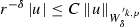. Further, as proved in [20], $\lim _{r\rightarrow 0} r^{-\delta } \left| u\right| = \lim _{r \rightarrow \infty } r^{-\delta } \left| u\right| =0$.

Let $M$ be a smooth, connected, complete, $n$-dimensional Riemannian manifold $(M,\gamma )$, and let $\rho <0$. We say $(M,\gamma )$ is asymptotically Euclidean of class $W^{'k,p}_{\rho }$ if

• The metric $\gamma \in W^{'k,p}_{\rho }(M)$, where $1/p-k/n<0$ and $\gamma$ is continuous.

• There exists a finite collection $\{N_i\}_{i=1}^m$ of open subsets of $M$ and diffeomorphisms $\varPhi _i:E_r\rightarrow N_i$ ($E_r={\mathbb {R}}^n \backslash \bar{B}_r(0)$) such that $M-\cup _iN_i$ is compact.

• For each $i$, $\varPhi ^*_i\gamma -\bar{\gamma }\in W^{'k,p}_{\rho }(E_r)$

We call the charts $\varPhi _i$ end charts and the corresponding coordinates are end coordinates. Now, suppose $(M,\gamma )$ is asymptotically Euclidean, and let $\{\varPhi _i\}_{i=1}^{m}$ be its collection of end charts. Let $K=M-\cup _i\varPhi _i(E_{2r})$, so $K$ is a compact manifold. The weighted Sobolev space $W^{k,p}_{\delta }(M)$ is the subset of $W^{k,p}_{\text {loc}}(M)$ such that the norm

(96)

is finite. We can define similarly weighted Lebesgue space $L^{'p}_{\delta }(M)$ and $C^{'k}_{\delta }$ and $C^{'\infty }_{\delta }(M)=\cap _{k=0}^{\infty }C^{'k}_{\delta }(M)$. In the particular case when $M={\mathbb {R}}^n$, then we have just one asymptotically Euclidean end. Moreover, if $(M,\gamma )$ is an asymptotically Euclidean manifold of class $W^{'k,p}_{\rho }$, we say $(M,\gamma ,K)$ is asymptotically Euclidean dataset if $K\in W^{'k-1,p}_{\rho -1}(M)$.

The main goal of this appendix is to consider the Poisson operator ${\mathcal {L}}=\varDelta _{\gamma }-\alpha$ on scalar functions of an asymptotically Euclidean manifold and express a very classical result ([33] or see [32]), that is, ${\mathcal {L}}$ is an isomorphism from Sobolev space $W^{'2,p}_{\delta }$ to $L^{'p}_{\delta }$. We start with the estimate [8, 9, 32]

Lemma 3

Suppose $(M,\gamma )$ is asymptotically Euclidean of class $W^{'2,p}_{\rho }$, $p>\frac{n}{2}$, $\rho <0$. Then if $2-n<\delta <0$, $\delta '\in {\mathbb {R}}$, and $u\in W^{'2,p}_{\delta }$ we have

(97)

Now we have following weak maximum principle (Lemma 3.2 in [32])

Lemma 4

Suppose $(M,\gamma )$ is asymptotically Euclidean of class $W^{'k,p}_{\rho }$, $k\ge 2$, $k>\frac{n}{p}$, and suppose $\alpha \in W^{'k-2,p}_{\rho -2}$ and suppose $\alpha \ge 0$. If $u\in W^{'k,p}_{\text {loc}}$ satisfies

$$\begin{aligned} -\!\varDelta _{\gamma } u+\alpha u\le 0 \end{aligned}$$

(98)

and if $u^+\equiv \text {max}(u,0)$ is $o(1)$ on each end of $M$, then $u\le 0$. In particular, if $u\in W^{'k,p}_{\delta }$ for some $\delta <0$ and $u$ satisfies (98), then $u\le 0$.

Proof

Fix $\epsilon >0$, and let $v=(u-\epsilon )^+$. Since $u^+=o(1)$ on each end, we see $v$ is compactly supported. Moreover, since $u\in W^{'k,p}_{\text {loc}}$ we have from Sobolev embedding that $u\in W^{'1,2}_{\text {loc}}$ and hence $v\in W^{'1,2}$. Now,

$$\begin{aligned} \int _M \left( -v\varDelta _{\gamma } u+\alpha uv\right) \, \text {d}x\le 0\quad \Longrightarrow \quad \int _M -v\varDelta _{\gamma } u\, \text {d}x \le -\int _M\alpha uv \, \text {d}x\le 0 \end{aligned}$$

(99)

where $\text {d}x$ denotes the volume element on $(M,\gamma )$. Since $\alpha \ge 0$, $v\ge 0$ and u is positive wherever $v\ne 0$. Integrating by parts we have

$$\begin{aligned} \int _M\left| \nabla v\right| ^2\, dx\le 0 \end{aligned}$$

(100)

since $\nabla u=\nabla v$ on the support of $v$. So $v$ is constant and compactly supported, so it should be zero, i.e. $\text {max}(u-\epsilon ,0)=0$. Then we conclude $u\le \epsilon$. Sending $\epsilon$ to $0$ we have $u\le 0$.

Now, if $u\in W^{'k,p}_{\delta }$, since $W^{'k,p}_{\delta }\subset C^{'0}_{\delta }$,, we have $u\in C^{'0}_{\delta }$. Hence if $\delta <0$, then $u^+=o(1)$ and lemma can be applied to $u$. $\square$

Using this lemma we can prove the following theorem.

Theorem 2

Suppose $(M,\gamma )$ is asymptotically Euclidean of class $W^{'2,p}_{\rho }$, $p>\frac{n}{2}$. Then if $2-n<\delta <0$ and $\alpha \in L'^p_{\delta -2}$, the operator ${\mathcal {L}}:W^{'2,p}_{\delta }\rightarrow L^{'p}_{\delta -2}$ is Fredholm with index $0$. Moreover, if $\alpha \ge 0$ then ${\mathcal {L}}$ is an isomorphism.

Proof

By the estimate in Lemma 3 and [9] this operator is Fredholm. Now we show ${\mathcal {L}}$ is injective. Let ${\mathcal {L}}u=0$ for $u\in W^{'2,p}_{\delta }$. Then by weak maximum principle we have $u=0$ on $M$ for $2-n<\delta <0$ and ${\mathcal {L}}$ is injective. To show ${\mathcal {L}}$ is surjective, it suffices to show ${\mathcal {L}}^*$ is injective from $L^{'p}_{2-n-\delta }\rightarrow W^{'-2,p}_{-n-\delta }$. Now let $f_1$ and $f_2$ be smooth and compactly supported in each end of $M$. We have from integration by parts

$$\begin{aligned} 0=\left<f_2,{\mathcal {L}}^*(f_1)\right>=\left<{\mathcal {L}}(f_2),f_1\right>=\int _M {\mathcal {L}}(f_2)f_1\, \text {d}x \end{aligned}$$

(101)

Thus $\int _M {\mathcal {L}}(f_2)f_1\, \text {d}x=0$ for all smooth and compactly supported $f_2$ in each end of $M$, then $f_1=0$ and ${\mathcal {L}}^*$ is injective. Then ${\mathcal {L}}$ is surjective. Therefore, ${\mathcal {L}}$ is an isomorphism. $\square$

Appendix B: Myers–black hole initial data

In this Appendix we will give details on various properties of the initial data for the extreme Myers–Perry metric. We have used MAPLE to simplify a number of our computations. Our main interest is to find certain final bounds and since most of the calculations are similar, we only provide explicit details for a subset of cases. The slice metric can be written as

$$\begin{aligned} h=\frac{\varSigma }{r^2}\left( dr^2 + r^2 \text {d}\theta ^2\right) +\sigma _{ij}\text {d}\phi ^i\text {d}\phi ^j \end{aligned}$$

(102)

where

$$\begin{aligned} \varSigma&= r^2+ab+a^2\cos ^2\theta +b^2\sin ^2\theta \qquad \quad \sigma _{12}=\frac{ab\mu }{\varSigma }\sin ^2\theta \cos ^2\theta \nonumber \\ \sigma _{11}&= \frac{a^2\mu }{\varSigma }\sin ^4\theta +(r^2+ab+a^2)\sin ^2\theta \nonumber \\ \sigma _{22}&= \frac{b^2\mu }{\varSigma }\cos ^4\theta +(r^2+ab+b^2)\cos ^2\theta \end{aligned}$$

(103)

where $\phi ^1=\varphi$ and $\phi ^2=\psi$. Now if we choose $\rho =\frac{1}{2}r^2\sin 2\theta$ and $z=\frac{1}{2}r^2\cos 2\theta$, then the conformal slice metric of the extreme Myers–Perry black hole can be written

$$\begin{aligned} \tilde{h}=e^{2U}\left( \text {d}\rho ^2 + \text {d}z^2\right) +\sigma '_{ij}\text {d}\phi ^i\text {d}\phi ^j \end{aligned}$$

(104)

where

$$\begin{aligned} \varPhi _0^2=\frac{\sqrt{\det \sigma }}{\rho }\qquad \sigma '_{ij}=\varPhi _0^{-2}\sigma _{ij}\qquad e^{2U}=\varPhi _0^{-2}\frac{\varSigma }{r^4} \end{aligned}$$

(105)

In general, the lapse and shift vectors are degrees of freedom for the initial data set. But since we want to preserve geometrical properties of the initial data under evolution, we compute the lapse of the extreme Myers–Perry spacetime and select the shift vector to be the product of $r$ and the shift of the extreme Myers–Perry metric.

$$\begin{aligned} \alpha&= \sqrt{\frac{r^4\varSigma }{(\varSigma +\mu )r^4+\mu ^2\left( r^2+ab\right) }},\end{aligned}$$

(106)

$$\begin{aligned} \beta ^{\varphi }&= \frac{ra\mu (r^2+ab+b^2)}{(\varSigma +\mu )r^4+\mu ^2\left( r^2+ab\right) },\nonumber \\ \beta ^{\psi }&= \frac{rb\mu (r^2+ab+a^2)}{(\varSigma +\mu )r^4+\mu ^2\left( r^2+ab\right) } \end{aligned}$$

(107)

In addition, we showed in Sect. 2.2 that the extrinsic curvature can be generated from scalar potentials $\omega _{\phi ^i}$. In the coordinate system used above, these are

$$\begin{aligned} \omega _{\varphi }&= \frac{a(a^2-b^2)(r^2+ab+b^2)\cos ^2\theta -r^2a(2a^2+2ab+r^2)}{(a-b)^2}\nonumber \\&\quad +\frac{a(r^2+ab+a^2)^2(r^2+ab+b^2)}{\varSigma (a-b)^2}\end{aligned}$$

(108)

$$\begin{aligned} \omega _{\psi }&= \frac{br^2((a+b)^2+r^2)-b(a^2-b^2)(r^2+ab+a^2)\cos ^2\theta }{(a-b)^2}\nonumber \\&\quad -\frac{b(r^2+ab+a^2)(r^2+ab+b^2)^2}{\varSigma (a-b)^2} \end{aligned}$$

(109)

It is important to mention

$$\begin{aligned} \varDelta _2=\frac{\partial ^2}{\partial \rho ^2}+\frac{\partial ^2}{\partial z^2}=\frac{1}{r^4}\left( r^2\frac{\partial ^2}{\partial r^2}+r\frac{\partial }{\partial r}+\frac{\partial ^2}{\partial \theta ^2}\right) \end{aligned}$$

(110)

Now we will prove some useful lemmas for the main theorem.

Lemma 5

The function $\alpha$ in Eq. (92) is nonnegative and has the following bounds

$$\begin{aligned} \alpha =\frac{\tilde{K}^{2}_{0}}{2\varPhi _0^6}+\frac{r^2}{4}(dv)^2=hr^{-6} \end{aligned}$$

(111)

where $h$ is a bounded nonnegative function.

Proof

First we know by conformal transformation $h_{ab}=\varPhi ^2\tilde{h}_{ab}$ the scalar curvature will be

$$\begin{aligned} \tilde{R}=R\varPhi ^2+3\varDelta _{\tilde{h}}v+\frac{3}{2}|\tilde{\nabla } v|^2 \end{aligned}$$

(112)

where $v=2\log \varPhi$. By constraint Eq. (47) and the fact that conformal extreme Myers–Perry satisfies in relation

$$\begin{aligned} \varDelta _{\tilde{h}}v=-\frac{1}{\varPhi ^6}\tilde{K}_{ab}\tilde{K}^{ab} \end{aligned}$$

(113)

we have

$$\begin{aligned} \tilde{R}&= {K}_{ab}{K}^{ab}\varPhi ^2-3\tilde{K}_{ab}\tilde{K}^{ab}+\frac{3}{2}|\tilde{\nabla } v|^2\nonumber \\&= -2\tilde{K}_{ab}\tilde{K}^{ab}\varPhi ^{-6}+\frac{3}{2}e^{-2U}(dv)^2 \end{aligned}$$

(114)

Then by Eq. (54) and (55) we have

$$\begin{aligned} \tilde{R}_0=-2\tilde{K}^2_0\varPhi ^{-6}+\frac{3r^2}{2}(dv)^2 \end{aligned}$$

(115)

Therefore, $\alpha$ is

$$\begin{aligned} \alpha =\frac{\tilde{R}_{0}}{6}+\frac{5\tilde{K}^{2}_{0}}{6\varPhi _0^6}=\frac{\tilde{K}^{2}_{0}}{2\varPhi _0^6}+\frac{r^2}{4}(dv)^2=hr^{-6} \end{aligned}$$

(116)

$\square$

Lemma 6

Let $\varPhi _0$, $\tilde{R}_0$, and $\tilde{K}^2_0$ be defined as in (105), (54), and (56), respectively. Then we have the following bounds:

• 1. $(ab\mu )^{1/4}\le \left[ (r^2+ab+b^2)(r^2+ab+a^2)\right] ^{1/4}\le r\varPhi _0 \le \big [(r^2+ab+b^2)(r^2+ab+a^2)+\mu ^2\big ]^{1/4}$

• 2. $\left| \tilde{R}_0\right| \le \frac{C}{r^4}$ and $\left| \tilde{K}^2_0\right| \le \frac{C}{r^6}$

• 3. $|\varDelta _4\varPhi _0|\le \frac{C}{r^6}$

Proof

We will prove just 1 here; the remaining bounds require lengthy algebraic manipulations.

• 1. We have

  $$\begin{aligned} r^2\varPhi _0^2&= \left[ (r^2+ab+b^2)(r^2+ab+a^2)\right. \nonumber \\&\quad \left. +\frac{\mu (r^2+ab)(a^2\cos ^2\theta +b^2\sin ^2\theta )+\mu a^2b^2}{\varSigma }\right] ^{1/2}\nonumber \\&\le \left[ (r^2+ab+b^2)(r^2+ab+a^2)+\mu ^2\right] ^{1/2} \end{aligned}$$

  (117)

  so if $r\rightarrow \infty$ then we have minimum of $r^2\varPhi _0^2$

  $$\begin{aligned} \sqrt{(r^2+ab+b^2)(r^2+ab+a^2)}\le r^2\varPhi _0^2 \end{aligned}$$

  (118)

  Therefore for $a,b>0$ we have

  $$\begin{aligned} (ab\mu )^{1/4}&\le \left[ (r^2+ab+b^2)(r^2+ab+a^2)\right] ^{1/4}\le r\varPhi _0\nonumber \\&\le \left[ (r^2+ab+b^2)(r^2+ab+a^2)+\mu ^2\right] ^{1/4} \end{aligned}$$

  (119)

$\square$

Lemma 7

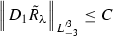
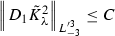
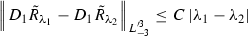
If we transform metric functions by (57) for small $\lambda$ (i.e.$-\lambda _0 < \lambda < \lambda _0$) then

• 1.
• 2.
• 3.
• 4.
• 5.
• 6.

Proof

We will prove numbers 1 and 4 of these inequalities and others will be similar. 1) By definition of $\tilde{R}_{\lambda }$ we have

$$\begin{aligned} \tilde{R}_{\lambda }&= -r^2\varDelta _2(U+\lambda U_1)+r^2\frac{\det (\text {d}\sigma '+\lambda \text {d}\bar{\sigma })}{2\rho ^2}=-r^2\varDelta _2 U-r^2\lambda \varDelta _2 U_1\nonumber \\&\quad +\frac{r^2}{2\rho ^2}\left[ (\text {d}\sigma '_{11}+\lambda \text {d}\bar{\sigma }_{11})\cdot (\text {d}\sigma '_{22}+\lambda \text {d}\bar{\sigma }_{22})-(\text {d}\sigma '_{12}+\lambda \text {d}\bar{\sigma }_{12})^2\right] \nonumber \\&= \tilde{R}_0-r^2\lambda \varDelta _2 U_1\nonumber \\&\quad +\frac{r^2}{2\rho ^2}\left[ \lambda \text {d}\bar{\sigma }_{11}\cdot \text {d}\sigma '_{22}+\lambda (\text {d}\sigma '_{11}+\lambda \text {d}\bar{\sigma }_{11})\cdot \text {d}\bar{\sigma }_{22}-\lambda (2\text {d}\sigma '_{12}+\lambda \text {d}\bar{\sigma }_{12})\cdot \text {d}\bar{\sigma }_{12}\right] \nonumber \\ \end{aligned}$$

(120)

Then by triangle inequality we have

(121)

We used inequality of Lemma 2–6 and the fact that functions ${U}_1$ and $\bar{\sigma }_{ij}$ have compact support outside the origin.

4) By definition of full contraction of extrinsic curvature we have

$$\begin{aligned} \tilde{K}^2_{\lambda }&= \frac{r^2}{2\rho ^4}\Bigg [(\sigma '_{11}+\lambda \bar{\sigma }_{11})(\text {d}\omega _{\psi }+\lambda \text {d}\omega _{2})^2+(\sigma '_{22}+\lambda \bar{\sigma }_{22})(\text {d}\omega _{\varphi }+\lambda \text {d}\omega _{1})^2\nonumber \\&\quad -2(\sigma '_{12}+\lambda \bar{\sigma }_{12})(\text {d}\omega _{\psi }+\lambda \text {d}\omega _{2})\cdot (\text {d}\omega _{\varphi }+\lambda \text {d}\omega _{1})\Bigg ] \end{aligned}$$

(122)

Then have

$$\begin{aligned} D_1\tilde{K}^2_{\lambda }&= \frac{r^2}{2\rho ^4}\Bigg [\bar{\sigma }_{11}(\text {d}\omega _{\psi }+\lambda \text {d}\omega _{2})^2+2(\sigma '_{11}+\lambda \bar{\sigma }_{11})\text {d}\omega _{2}\cdot (\text {d}\omega _{\psi }+\lambda \text {d}\omega _{2})+\bar{\sigma }_{22}(\text {d}\omega _{\varphi }\nonumber \\&\quad +\lambda \text {d}\omega _{1})^2 +(\sigma '_{22}+\lambda \bar{\sigma }_{22})\text {d}\omega _{1}\cdot (\text {d}\omega _{\varphi }+\lambda \text {d}\omega _{1})-2\lambda \bar{\sigma }_{12}(\text {d}\omega _{\psi }\nonumber \\&\quad +\lambda \text {d}\omega _{2})\cdot (\text {d}\omega _{\varphi }+\lambda \text {d}\omega _{1})-4(\sigma '_{12}+\lambda \bar{\sigma }_{12})\lambda \text {d}\omega _{2}\cdot (\text {d}\omega _{\varphi }+\lambda \text {d}\omega _{1})\nonumber \\&\quad -4(\sigma '_{12}+\lambda \bar{\sigma }_{12})(\text {d}\omega _{\psi }+\lambda \text {d}\omega _{2})\cdot \text {d}\omega _{1}\Bigg ] \end{aligned}$$

(123)

Then by the triangle inequality and the fact that $\omega _i$ has compact support outside axis and $\bar{\sigma }_{ij}$ has compact support outside the origin one can show it is bounded. $\square$

Finally,we have following limits

$$\begin{aligned} \lim _{s\rightarrow \infty } \omega _{\varphi }&= \frac{ab\mu \cos ^2\theta }{(a-b)}+\frac{a^3b\mu (a+b)}{(ab+a^2\cos ^2\theta +b^2\sin ^2\theta )(a-b)^2}\end{aligned}$$

(124)

$$\begin{aligned} \lim _{s\rightarrow \infty } \omega _{\psi }&= -\frac{ab\mu \cos ^2\theta }{(a-b)}-\frac{ab\mu (a+b)}{(ab+a^2\cos ^2\theta +b^2\sin ^2\theta )(a-b)^2}\end{aligned}$$

(125)

$$\begin{aligned} \lim _{s\rightarrow \infty } r\varPhi _0&= \frac{\mu (\mu -ab)}{2(ab+a^2\cos ^2\theta +b^2\sin ^2\theta )}. \end{aligned}$$

(126)

References

Alaee, A., Kunduri, H.K., Pedroza, E.M.: Notes on maximal slices of five-dimensional black holes. Class. Quantum Gravity 31(5), 055,004 (2014). http://stacks.iop.org/0264-9381/31/i=5/a=055004
Amsel, A.J., Horowitz, G.T., Marolf, D., Roberts, M.M.: Uniqueness of extremal Kerr and Kerr–Newman black holes. Phys. Rev. D81, 024,033 (2010). doi:10.1103/PhysRevD.81.024033
Aretakis, S.: Stability and instability of extreme reissner-nordström black hole spacetimes for linear scalar perturbations i. Commun. Math. Phys. 307(1), 17–63 (2011)
Aretakis, S.: Horizon instability of extremal black holes (2012). arXiv:1206.6598
Bartnik, R.: The mass of an asymptotically flat manifold. Commun. Pure Appl. Math. 39(5), 661–693 (1986)
Bartnik, R., Isenberg, J.: The constraint equations. In: The Einstein equations and the large scale behavior of gravitational fields, pp. 1–38. Springer (2004)
Beig, R., Chrusciel, P.T.: Killing initial data. Class. Quantum Gravity 14(1A), A83 (1997)
Choquet-Bruhat, Y.: General Relativity and the Einstein Equations. Oxford University Press, UK (2009)
Choquet-Bruhat, Y., Christodoulou, D.: Elliptic systems inh s, \(\delta \) spaces on manifolds which are Euclidean at infinity. Acta Math. 146(1), 129–150 (1981)
Choquet-Bruhat, Y., Isenberg, J., York Jr, J.W.: Einstein constraints on asymptotically Euclidean manifolds. Phys. Rev. D 61(8), 84,034 (2000)
Choquet-Bruhat, Y., York Jr, J.W.: The cauchy problem. In: Held, A. (ed.) General Relativity and Gravitation. One Hundred Years After the Birth of Albert Einstein, vol. 1, p. 99. Plenum Press, New York, NY (1980)
Chrusciel, P., Mazzeo, R.: Initial data sets with ends of cylindrical type: I. the lichnerowicz equation, (2012). arXiv preprint arXiv:1201.4937
Chrusciel, P., Mazzeo, R., Pocchiola, S.: Initial data sets with ends of cylindrical type: Ii the vector constraint equation, (2012). arXiv preprint arXiv:1203.5138
Chruściel, P.T., Costa, J.L.: Mass, angular-momentum and charge inequalities for axisymmetric initial data. Class. Quantum Gravity 26(23), 235,013 (2009)
Dain, S.: Initial data for a head-on collision of two Kerr-like black holes with close limit. Phys. Rev. D 64(12), 124,002 (2001)
Dain, S.: Proof of the (local) angular momentum-mass inequality for axisymmetric black holes. Class. Quantum Gravity 23(23), 6845 (2006)
Dain, S.: Axisymmetric evolution of Einstein equations and mass conservation. Class. Quantum Gravity 25(14), 145,021 (2008)
Dain, S.: Proof of the angular momentum-mass inequality for axisymmetric black holes. J. Diff. Geom 79, 33–67 (2008)
Dain, S.: Geometric inequalities for axially symmetric black holes. Class. Quantum Gravity 29(7), 073,001 (2012)
Dain, S., Gabach Clement, M.E.: Small deformations of extreme Kerr black hole initial data. Class. Quantum Gravity 28, 075,003 (2011). doi:10.1088/0264-9381/28/7/075003
Dias, O.J., Figueras, P., Monteiro, R., Santos, J.E.: Ultraspinning instability of rotating black holes. Phys. Rev. D82, 104,025 (2010). doi:10.1103/PhysRevD.82.104025
Figueras, P., Kunduri, H.K., Lucietti, J., Rangamani, M.: Extremal vacuum black holes in higher dimensions. Phys. Rev. D78, 044,042 (2008). doi:10.1103/PhysRevD.78.044042
Figueras, P., Lucietti, J.: On the uniqueness of extremal vacuum black holes. Class. Quantum Gravity 27, 095,001 (2010). doi:10.1088/0264-9381/27/9/095001
Figueras, P., Murata, K., Reall, H.S.: Black hole instabilities and local penrose inequalities. Class. Quantum Gravity 28(22), 225,030 (2011)
Hollands, S.: Horizon area-angular momentum inequality in higher-dimensional spacetimes. Class. Quantum Gravity 29(6), 065,006 (2012)
Hollands, S., Ishibashi, A.: On the ‘stationary implies axisymmetric’ theorem for extremal black holes in higher dimensions. Commun. Math. Phys. 291, 403–441 (2009). doi:10.1007/s00220-009-0841-1
Isenberg, J.: Constant mean curvature solutions of the Einstein constraint equations on closed manifolds. Class. Quantum Gravity 12(9), 2249 (1995)
Kunduri, H.K., Lucietti, J.: A classification of near-horizon geometries of extremal vacuum black holes. J. Math. Phys. 50(8), 082,502 (2009)
Kunduri, H.K., Lucietti, J.: Classification of near-horizon geometries of extremal black holes. Living Rev. Rel. 16, 8 (2013). doi:10.12942/lrr-2013-8
Lucietti, J., Murata, K., Reall, H.S., Tanahashi, N.: On the horizon instability of an extreme Reissner–Nordstrom black hole. JHEP 1303, 035 (2013). doi:10.1007/JHEP03(2013)035
Lucietti, J., Reall, H.S.: Gravitational instability of an extreme Kerr black hole. Phys. Rev. D 86(10), 104,030 (2012)
Maxwell, D.: Solutions of the Einstein constraint equations with apparent horizon boundaries. Commun. Math. Phys. 253(3), 561–583 (2005)
McOwen, R.C.: The behavior of the Laplacian on weighted sobolev spaces. Commun. Pure Appl. Math. 32(6), 783–795 (1979)
Murata, K., Reall, H.S., Tanahashi, N.: What happens at the horizon(s) of an extreme black hole? Class. Quant. Grav. 30, 235,007 (2013). doi:10.1088/0264-9381/30/23/235007
Myers, R.C.: Myers–perry black holes, (2011). arXiv preprint arXiv:1111.1903 (2011)
Myers, R.C., Perry, M.: Black holes in higher dimensional space-times. Ann. Phys. 172(2), 304–347 (1986)
Pomeransky, A., Sen’kov, R.: Black ring with two angular momenta (2006). arXiv preprint hep-th/0612005
Reiris, M.: Instability of the extreme kerr-newman black-holes, (2013). arXiv preprint arXiv:1311.3156
Acknowledgments
AA is supported by a graduate scholarship from Memorial University. HKK is supported by an NSERC Discovery Grant. We would like to thank Ivan Booth and Chris Radford for useful comments and discussions. We also especially thank Sergio Dain and Eugenia Gabach-Clement for reading a draft of the manuscript and for a number of helpful suggestions and comments. This research was supported in part by Perimeter Institute for Theoretical Physics. Research at Perimeter Institute is supported by the Government of Canada through Industry Canada and by the Province of Ontario through the Ministry of Economic Development and Innovation.
Author information
Authors and Affiliations
Corresponding author