A theoretical and computational investigation of mixed mode creep crack growth along an interface

Abstract

In this paper, we propose a theoretical framework for studying mixed mode (I and II) creep crack growth under steady state creep conditions. In particular, we focus on the problem of creep crack growth along an interface, whose fracture properties are weaker than the bulk material, located either side of the interface. The theoretical framework of creep crack growth under mode I, previously proposed by the authors, is extended. The bulk behaviour is described by a power-law creep, and damage zone models that account for mode mixity are proposed to model the fracture process ahead of a crack tip. The damage model is described by a traction-separation rate law that is defined in terms of effective traction and separation rate which couple the different fracture modes. Different models are introduced, namely, a simple critical displacement model, empirical Kachanov type damage models and a micromechanical based model. Using the path independence of the $C^{*}$-integral and dimensional analysis, analytical models are developed for mixed mode steady-state crack growth in a double cantilever beam specimen (DCB) subjected to combined bending moments and tangential forces. A computational framework is then implemented using the Finite Element method. The analytical models are calibrated against detailed Finite Element models and a scaling function ($C_{k}$) is determined in terms of a dimensionless quantity $\phi _{0}$ (which is the ratio of geometric and material length scales), mode mixity $\chi$ and the deformation and damage coupling parameters. We demonstrate that the form of the $C_{k}$-function does not change with mode mixity; however, its value depends on the mode mixity, the deformation and damage coupling parameters and the detailed form of the damage zone. Finally, we demonstrate how parameters within the models can be obtained from creep deformation, creep rupture and crack growth experiments for mode I and II loading conditions.

1 Introduction

In many engineering applications at elevated temperature, structural components exhibit significant time-dependent inelastic deformation, which might lead to nucleation and/or propagation of flaws. Studying creep crack growth (CCG) has been an active area of research over the last four decades, with the aim of designing structures with high integrity and safety. In this paper, we aim to devise analytical models for steady-state crack growth under mixed mode loading conditions which can be calibrated against detailed Finite Element simulations. Such models can be used to investigate the effect of different material parameters and damage models on the crack growth behaviour under complex loading conditions.

The majority of early studies on creep crack growth focused on pure mode I loading conditions, with the aim of developing a parameter that characterises the near crack tip fields as well as crack propagation. The so called $C^{*}$-integral (Landes and Begley 1976; Nikbin et al. 1976; Ohji et al. 1976), i.e. the creep J-integral (Rice 1978), was introduced to characterise the crack tip fields and creep crack growth under steady state creep conditions. In particular, it provides descriptions of the strain-rate and stress singularities at the crack tip and a correlation of experimental crack growth rate data (Taira et al. 1979; Riedel and Rice 1980). Moreover, the $C^{*}$-integral is path independent for contours in which the material properties only vary in the direction perpendicular to the direction of crack growth within the family of contours considered. Under transient conditions, i.e. the transition from short-time elastic to long-time creep, other parameters such as C(t), $C_{t}$ and $C^{*}_{\mathrm {h}}$ are found to characterise both stationary and propagating cracks with a variable degree of suitability (Riedel and Rice 1980; Riedel 1981; Saxena 1986).

Under mixed mode loading and steady state conditions, the $C^{*}$-integral remains a valid parameter (Chambers et al. 1992). Chambers et al. (1992) assumed that only a part of the $C^{*}$-integral, i.e. that part related to mode I, is responsible for propagating the crack. They defined the damage at the crack tip by a function of the von Mises equivalent stress and then used the amplitude of the singular von Mises stress field to determine an effective value of $C^{*}$ by comparing mode I and mixed mode loading conditions. Further, under transient creep conditions, the role of mode mixity on the stress field ahead of a crack tip was investigated by Brockenbrough et al. (1991) using the C(t) parameter.

The damage process ahead of a propagating crack tip in polycrystalline materials under creep conditions is controlled by the formation of discrete voids or micro cracks at grain boundaries. As these voids and/or micro cracks grow and coalesce, they form secondary cracks which coalesce creating the new crack surfaces, allowing the primary macroscopic crack to advance along an interface or interconnected grain-boundaries (Riedel 1987). These secondary cracks are usually not perpendicular to the loading direction, which can generate mixed mode loading conditions locally at the crack tip. In some materials, an extensive damage zone can develop in the vicinity of a crack tip in which many boundaries are cavitated. The interaction between these different cavitated and microcracked regions is important and can lead to a significant reduction of stress locally and macroscopic dilation (i.e. diffused damage). In other materials, damage is confined to a small region directly ahead of the crack tip such that the dilation due to the growth of the damage is then very localised. In the presence of interfaces, whose fracture properties are weaker than the bulk material, e.g. in dissimilar metal welds (Yamazaki et al. 2008; Laha et al. 2012; Hu et al. 2019), a crack might be forced to grow along an interface, which might lead to mixed mode loading at the crack tip, regardless of the global loading conditions. Mode mixity can influence damage development.

The mode mixity effect is usually incorporated using effective measures such as the effective stress, effective creep strain, or accumulated creep strain at a critical distance ahead of the crack tip. In these models the deformation of the bulk material is assumed not to be influenced by the presence of damage. Using empirical Kachanov type continuum damage mechanics models (Kachanov 1958; Rabotnov 1969), the single scalar damage parameter is assumed to be determine by the stress state which allows the effect of mode mixity to be taken into account (Nikbin et al. 1976, 1984; Yatomi and Nikbin 2014). The development of the damage process zone at a crack tip has been modelled by Onck and van der Giessen (Onck and van der Giessen 1998; Van Der Giessen and Tvergaard 1994) using the Finite Element Method, together with both mechanistic and empirical models. The latter models fully describe the interaction between deformation and damage development and account for mode mixity. In these models, the contribution of the different fracture modes (i.e. the coupling) to the deformation and the damage in the damage zone are assumed to be the same.

Another method of modelling crack propagation is through the use of interface cohesive or damage zone models. Interface damage zone models of this type provide a coupling between the local separation rate across an interface and bulk deformation processes. They introduce a physically meaningful length scale that is related to the dissipative mechanisms responsible for damage development. Damage zone models of this type describe the fracture process in the vicinity of the crack tip as a gradual surface separation process, such that the normal and shear traction at the interface resist separation and relative sliding. The cohesive/damage zone modelling approach has its origins in the pioneering work of Dugdale (1960) and Barenblatt (1962) and was later implemented in a Finite Element environment by Hillerborg et al. (1976). Several models have been proposed in the literature, wherein a variety of materials and applications have been successfully investigated (Camacho and Ortiz 1996; Corigliano et al. 2003; Elmukashfi and Kroon 2014; Hui et al. 1992; Knauss 1993; Needleman 1987, 1990; Rahul-Kumar et al. 1999; Rice and Wang 1989; Tvergaard 1990; Xu and Needleman 1993). These first attempts focused on studying the mode I fracture process, i.e. the relation between the traction and separation that are normal to the fracture surface. Later, it was extended to mode II fracture, in which the tangential traction and sliding are defined. In modelling mixed mode loading conditions, two approaches are often used to define the interaction between different fracture modes. The first approach is by fully coupling the normal and tangential components of the traction and separation through introducing an effective traction and/or separation parameters (Tvergaard and Hutchinson 1996; Pardoen et al. 2005). The damage is evaluated using a representative separation that determines the contribution of the different fracture modes and yields different fracture energies for the different modes. The second approach assumes uncoupled behaviour between the different modes, i.e. uncoupled normal and tangential deformation, but the total fracture energy is taken to be the sum of the fracture energy components of the different modes (Kafkalidis and Thouless 2002; Li et al. 2006). Experimental studies show that the fracture process depends on the properties of the different materials, and the coupling between the different modes strongly depends on the nature of the process zone.

The objective of this paper is to study a simple geometry, in which we project the damage onto a single plane directly ahead of the crack tip, and a series of loading conditions to provide fundamental information about the effect of mode mix on crack growth. Simplifying the model in this way allows us to undertake a rigorous analysis that provides important insights that will ultimately help us to explore and explain more complicated and realistic scenarios. Therefore, we developed a theoretical and computational framework for creep crack growth under mixed mode conditions. The crack growth is assumed to be determined by the damage in a concentrated narrow zone directly ahead of the crack tip (i.e. the damage in not diffused in the bulk material) in a weak interface that is parallel to the crack. A theoretical framework is initially introduced in which the constitutive behaviour of the bulk material is described by a power-law creep and the damage zone model constitutive relation is described by a traction-separation rate law. The damage models are formulated in terms of effective traction and separation parameters to account for mode mixity effects. The damage process is assumed to be determined by a representative separation which determines the damage dependence on different modes. We propose three different types of models, i.e. a simple critical displacement model, Kachanov type empirical models and a micromechanical based interface model, as extensions to the pure mode I models described in Elmukashfi and Cocks (2017). We use the same approach as described in Elmukashfi and Cocks (2017). We initially evaluate the behaviour of a double cantilever beam specimen (DCB) of infinite length subjected to combined bending moments and tangential forces. For this type of specimen, $C^{*}$ remains constant as the crack grows and the crack growth rate eventually achieves a steady state. By exploring the steady state response, we can establish the relationship between the steady state crack growth rate, $C^{*}$ and characteristic material and geometric length scales. The resulting models can then be used to evaluate more complex loading conditions and geometries. For the double cantilever beam, reasonably straightforward analytical expressions can be obtained for $C^{*}$. In the steady state, we can invoke the path independence of the $C^{*}$-integral and choose contours in the far field and surrounding the damage zone. This allows simple analytical expressions for the crack growth rate to be determined, which can be expressed in terms of $C^{*}$, damage zone material parameters, a dimensionless scaling parameter that is a function of the ratio of characteristic geometric and material length scales, and mode mixity. We use the Finite Element Method to determine the magnitude of the scaling parameter.

The theoretical framework is presented in Sect. 2 and the damage zone models are developed in Sect. 3. The analysis of creep crack growth in the double cantilever beam specimen and the Finite Element implementation of the damage zone model are described in Sect. 4, with the crack growth results for the different interface models presented and discussed in Sect. 5. Having established the theoretical framework and structure of the crack growth laws, we evaluate the behaviour of more representative testing geometries in Sect. 5.

2 Theoretical analysis of mixed mode creep crack

In this section, we investigate the theoretical aspects of mixed mode creep crack propagation. In particular, we adopt the theoretical framework introduced in Elmukashfi and Cocks (2017) and consider mixed mode crack propagation in creeping materials under steady state conditions. A full description and evaluation of the nature of crack tip fields for stationary and growing cracks is provided in Elmukashfi and Cocks (2017) for mode I conditions. Here the focus is on mixed mode and mode II conditions, which has achieved much less attention in the literature. Crack propagation is assumed to take place along an interface whose fracture properties are weaker than the bulk material (i.e. the crack propagates along the interface regardless of the far field and local mode mixities). Further, the path independence property of $C^{*}$ will be used to obtain a direct relationship between the far field loading and the fracture process parameters. It should be noted that for crack growth in an elastic/creeping material, path independence of $C^{*}$ still holds provided the size of the zone in which elastic deformation is important is smaller than the size of the crack tip damage process zone (Hui and Riedel 1981).

Consider a body which contains a crack and is subjected to a constant far field loading, see Fig. 1. A common Cartesian coordinate system for the reference and deformed configurations $x_{i}$, $i=1,2,3$, is assumed. Directly ahead of the crack there is an interface along which the crack propagates. The bulk material is assumed to exhibit steady-state creep behaviour which is defined by the constitutive law

Fig. 1

The schematic of interface crack model in creeping solid. The figure illustrates the definition of the interface surface $\varGamma _{\mathrm {int}}$, inner path $\varGamma _{\mathrm {in}}$ and the outer path $\varGamma _{\mathrm {out}}$

$$\begin{aligned} \dot{\varepsilon }_{ij} = \dfrac{\partial \varPhi }{\partial \sigma _{ij}} = \frac{3}{2} \, \dot{\varepsilon }_0 \, \Big (\frac{\sigma _{\mathrm {e}}}{\sigma _0}\Big )^{n} \, \frac{s_{ij}}{\sigma _{\mathrm {e}}}, \end{aligned}$$

(1)

where $\sigma _{ij}$ is the Cauchy’s stress tensor, $\dot{\varepsilon }_{ij}$ is the strain rate tensor, $s_{ij}=\sigma _{ij}-\frac{1}{3} \sigma _{kk} \delta _{ij}$ is the stress deviator, $\sigma _{\mathrm {e}}$ is the von Mises equivalent stress, $\sigma _{0}$ is a reference stress, $\dot{\varepsilon }_{0}$ is the strain rate at the reference stress and n is the rate sensitivity parameter. $\varPhi$ is the stress potential

$$\begin{aligned} \varPhi = \dfrac{1}{n+1} \, \dot{\varepsilon }_{0} \sigma _{0} \left( \dfrac{\sigma _{\mathrm {e}}}{\sigma _{0}}\right) ^{n+1}. \end{aligned}$$

(2)

The energy dissipation rate per unit volume, $\dot{D}$, is given by

$$\begin{aligned} \dot{D} = \varPhi +\varPsi , \end{aligned}$$

(3)

where $\varPsi$ is the dual rate potential

$$\begin{aligned} \varPsi = \dfrac{n}{n+1} \, \dot{\varepsilon }_{0} \sigma _{0} \left( \dfrac{\dot{\varepsilon }_{\mathrm {e}}}{\dot{\varepsilon }_{0}}\right) ^{\frac{n+1}{n}}, \end{aligned}$$

(4)

and $\dot{\varepsilon }_{\mathrm {e}}=\sqrt{\frac{2}{3} \dot{\varepsilon }_{ij} \dot{\varepsilon }_{ij}}$.

In this paper, we limit our consideration to situations in which the creep properties in the bulk material either side of the interface are the same. In dissimilar metal welds different bulk materials with different properties exist either side of the interface. The results presented here can be readily extended to consider this more general situation, but in order to identify the major features of the crack growth behaviour under mixed mode loading conditions we focus on the response of this simpler configuration.

Damage grows along the interface, driven by the local stress, and the crack advances when the damage at a material point ahead of the crack achieves a critical value. Hence, separation occurs along the interface to create two surfaces as the crack advances. Therefore, a material point along the interface is defined by the two normal vectors $n_{i}^{+}$ and $n_{i}^{-}$, where $n_{i}^{+}=n_{i}^{-}$, i.e. the initially intact material point splits into two points with unit normals acting opposite to each other and into the material on either side of the interface. The displacement-rate jump across the damage zone and the corresponding traction are defined by the vectors $\dot{\delta }_{i} = \dot{u}_{i}^{+}-\dot{u}_{i}^{-}$, where $\dot{u}_{i}^{+}$ and $\dot{u}_{i}^{-}$ are the displacement rates either side of the interface, and $T_{i}^{+}=\sigma _{ij} \, n_{j}^{+}$ and $T_{i}^{-}=\sigma _{ij} \, n_{j}^{-}$, respectively.

The problem is analysed by equating the values of $C^{*}$ determined on the inner and outer contours in Fig. 1. The $C^{*}$-integral is defined as

$$\begin{aligned} C^{*} = \int \limits _{\varGamma } \varPsi \, \mathrm {d}x_2 - T_i \, \frac{\partial \dot{u}_i}{\partial x_1} \, \mathrm {d}s, \end{aligned}$$

(5)

where $\varGamma$ is an arbitrary contour around the tip of the crack with unit outward normal $n_{i}$, $T_{i} = \sigma _{ij} \, n_{j}$ is the traction on $\mathrm {d}s$ and $\dot{u}_{i}$ is the displacement rate. The $C^*$-integral in the outer path, $C^{*}_{\mathrm {out}}$, is determined by the far field loading. For an interface that extends along the $x_{1}$-axis, the $C^*$-integral along the inner path, $C^{*}_{\mathrm {in}}$, is then evaluated as

$$\begin{aligned} C^{*}_{\mathrm {in}} = \int \limits _{0}^{\dot{\delta }_{i}^{m}} T_{i} \, \mathrm {d}\dot{\delta }_{i}, \end{aligned}$$

(6)

where $\dot{\delta }^{\mathrm {m}}_{i}$ is the displacement rate at the tip of the crack and $T_{i}=T_{i}^{+}=-T_{i}^{-}$. In the case of mixed mode loading, the components of the traction and displacement rates tangential and normal to the interface are considered, i.e. $(T_{t},\dot{\delta }_{t})$ and $(T_{n},\dot{\delta }_{n})$, respectively, as illustrated in Fig. 2. We postulate that there is an effective traction $T_{\mathrm {e}}$ and an effective separation rate $\dot{\delta }_{\mathrm {e}}$, that can be used to represent the constitutive relationship for the interface. (The effective traction and effective separation rate are assumed to be functions of the traction and separation rate components, respectively). Note also that the effective traction and separation rate are power conjugates. Thus, an equivalent expression to $C^{*}_{\mathrm {in}}$ in Eq. (6) is

$$\begin{aligned} C^{*}_{\mathrm {in}} = \int \limits _{0}^{\dot{\delta }_{\mathrm {e}}^{\mathrm {m}}} T_{\mathrm {e}} \, \mathrm {d}\dot{\delta }_{\mathrm {e}}, \end{aligned}$$

(7)

where $\dot{\delta }_{\mathrm {e}}^{\mathrm{m}}$ is the effective displacement rate at the tip of the crack. The effective separation $\delta _{\mathrm {e}}$ is then defined as the integration of the effective rate, i.e. $\delta _{\mathrm {e}}(t)=\int _{0}^{t} \dot{\delta }_{\mathrm {e}} \, \mathrm {d}t$.

Fig. 2

The damage zone along the interface for mixed mode crack propagation: a schematic of the damage zone and the traction and separation vectors, $\mathbf{T}$ and ${\varvec{\delta }}$, respectively; and b the effective traction-separation rate $(T_{\mathrm {e}}\text {-}\dot{\delta }_{\mathrm {e}})$ and the effective separation rate-separation $(\dot{\delta }_{\mathrm {e}}\text {-}{\delta }_{\mathrm {e}})$ distribution along the damage zone. l is the length of the interface zone, $\delta ^{\mathrm {c}}_{\mathrm {e}}$ is the critical effective separation, $\delta ^{\mathrm {f}}_{\mathrm {e}}$ is the effective separation at failure, $\dot{\delta }^{\mathrm {m}}_{\mathrm {e}}$ is the maximum effective separation rate and $\sigma ^{\mathrm {c}}$ is the interface strengthd

Hence, a relationship between the far field loading and the behaviour of the interface can be determined using the path-independence of $C^{*}$, i.e. $C^{*}_{\mathrm {out}}= C^{*}_{\mathrm {in}}$.

3 Damage zone models for mixed mode creep crack growth

In this section, we introduce a number of different models to describe the response within the damage zone under mixed mode conditions. The traction-separation-rate law is assumed to take a direct power law relationship between the effective traction $T_{\mathrm {e}}$ and the effective separation rate $\dot{\delta }_{\mathrm {e}}$. We can express the resulting constitutive relationships in a similar form to that for power-law creep of the bulk described in Sect. 2. Thus, the constitutive model takes the following form

$$\begin{aligned} \dot{\delta }_{\mathrm {e}} = \dot{\delta }_{0} \left( \dfrac{T_{\mathrm {e}}}{T_{0}}\right) ^{m} \quad \text {and} \quad T_{\mathrm {e}} = T_{0} \left( \dfrac{\dot{\delta }_{\mathrm {e}}}{\dot{\delta }_{0}}\right) ^{\frac{1}{m}}, \end{aligned}$$

(8)

where $T_{0}$ is a reference traction (equivalent to $\sigma _{0}$ of Eq. (1)), $\dot{\delta }_{0}$ is the separation rate at this traction and m is an exponent (which can have a different value to n in Eq. (1)). Throughout this paper, we set $T_{0}=\sigma _{0}$, so that the two reference stress like quantities are the same. A traction potential, $\phi$, can now be defined as

$$\begin{aligned} \phi = \dfrac{1}{m+1} \, \dot{\delta }_{0} T_{0} \left( \dfrac{T_{\mathrm {e}}}{T_{0}}\right) ^{m+1}. \end{aligned}$$

(9)

It follows that the energy dissipation rate per unit area, $\dot{d}$, and dual separation rate potential, $\psi$, are, respectively, given by

$$\begin{aligned} \dot{d} = \phi +\psi , \end{aligned}$$

(10)

and

$$\begin{aligned} \psi = \dfrac{m}{m+1} \, \dot{\delta }_{0} T_{0} \left( \dfrac{\dot{\delta }_{\mathrm {e}}}{\dot{\delta }_{0}}\right) ^{\frac{m+1}{m}}. \end{aligned}$$

(11)

The constitutive relations can also be expressed in terms of the traction and separation rate components as

$$\begin{aligned} \dot{\delta }_{i} = \dfrac{\partial \phi }{\partial T_{i}} = \dot{\delta }_{0} \left( \dfrac{T_{\mathrm {e}}}{T_{0}}\right) ^{m} \, \dfrac{\partial T_{\mathrm {e}}}{\partial T_{i}}, \end{aligned}$$

(12)

and

$$\begin{aligned} T_{i} = \dfrac{\partial \psi }{\partial \dot{\delta }_{i}} = T_{0} \left( \dfrac{\dot{\delta }_{\mathrm {e}}}{\dot{\delta }_{0}}\right) ^{\frac{1}{m}} \, \dfrac{\partial \dot{\delta }_{\mathrm {e}}}{\partial \dot{\delta }_{i}}, \end{aligned}$$

(13)

where the index notation i denotes the normal and tangential directions, i.e. $i \in [t,n]$, which will be used in the subsequent descriptions.

In what follows, a range of traction-separation-rate laws are introduced for mixed mode conditions which generalise the models described by Elmukashfi and Cocks (2017).

3.1 Simple critical displacement model

A simple form of the effective traction can be taken in the form of the resultant traction, i.e. the square root of the sum of squares of the normal and tangential traction, $T_{t}$ and $T_{n}$, respectively. Thus, the effective traction can be written in the general form

$$\begin{aligned} T_{\mathrm {e}} = \sqrt{ \left( \dfrac{T_{t}}{\alpha _{t}}\right) ^{2}+\left( \dfrac{T_{n}}{\alpha _{n}}\right) ^{2}}, \end{aligned}$$

(14)

where $\alpha _{t}$ and $\alpha _{n}$ are parameters that define the coupling between tangential and normal deformation as illustrated in Fig. 3. Thus, the separation rates in Eq. (12) take the following form

Fig. 3

The effective traction in the traction space in the case of the simple critical displacement model. The plots represent constant effective traction $T_{\mathrm {e}}$ for different values of $\alpha _{t}/\alpha _{n}$

$$\begin{aligned} \dot{\delta }_{i} = \dot{\delta }_{0} \left( \dfrac{T_{\mathrm {e}}}{T_{0}}\right) ^{m} \, \dfrac{T_{i}}{\alpha _{i}^{2} \, T_{\mathrm {e}}}. \end{aligned}$$

(15)

Using this relation and the definition of effective traction in Eq. (14), the effective separation rate, $\dot{\delta }_{\mathrm {e}}$, can be determined as

$$\begin{aligned} \dot{\delta }_{\mathrm {e}} = \sqrt{ \left( \alpha _{t} \, \dot{\delta }_{t}\right) ^{2}+\left( \alpha _{n} \, \dot{\delta }_{n}\right) ^{2}}. \end{aligned}$$

(16)

The traction in Eq. (13) is then given by

$$\begin{aligned} T_{i} = T_{0} \left( \dfrac{\dot{\delta }_{\mathrm {e}}}{\dot{\delta }_{0}}\right) ^{\frac{1}{m}} \, \dfrac{\alpha _{i}^{2} \, \dot{\delta }_{i}}{\dot{\delta }_{\mathrm {e}}}. \end{aligned}$$

(17)

The coupling between the tangential and normal deformation in the interface is determined by the parameters $\alpha _{t}$ and $\alpha _{n}$ as illustrated in Fig. 3 and Eqs. (14)–(17).

We assume that the damage does not influence the separation rates and failure is achieved when a suitable separation measure achieves a critical value. Hence, we introduce a representative separation, $\hat{\delta }$, that is a function of the tangential and normal separations, i.e. $\hat{\delta }=\hat{\delta }(\delta _{t},\delta _{n})$, which can be used to define the local failure condition as $\hat{\delta }=\hat{\delta }_{\mathrm {f}}$ where $\hat{\delta }_{\mathrm {f}}$ is the representative separation at failure. It is worth mentioning that the traction $T_{t}$, $T_{n}$ and $T_{\mathrm {e}}$, become zero at the position where local failure is achieved. The form of the representative separation $\hat{\delta }$ determines the contribution of the different fracture modes to the damage process. For example, assuming that $\hat{\delta }=\delta _{\mathrm {e}}$, the parameters $\alpha _{t}$ and $\alpha _{n}$ determine the coupling between both the deformation and local failure. Moreover, other forms can also be used to define $\hat{\delta }$, for example, for the cases that mode I controls the damage process, $\hat{\delta }\approx \delta _{n}$.

3.2 Kachanov type empirical model

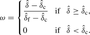
In this model, damage is assumed to influence the constitutive response. The damage is introduced using single or multiple scalar damage parameters, $\omega _{i}$, such that each parameter is assumed to evolve monotonically from 0 to 1, i.e. from an undamaged to a fully damaged state. We assume that the effective traction takes the quadratic form of Eq. (14) with the tangential, $T_{t}$, and normal, $T_{n}$, traction, replaced by $\bar{T}_{t}$ and $\bar{T}_{n}$, respectively, where, following Kachanov (1958) and Lemaitre and Chaboche (1994),

$$\begin{aligned} \bar{T}_{i} = \dfrac{T_{i}}{1-\omega _{i}}. \end{aligned}$$

(18)

Hence, the effective traction becomes

$$\begin{aligned} T_{\mathrm {e}} = \sqrt{ \left( \dfrac{T_{t}}{\alpha _{t} \left( 1-\omega _{t} \right) }\right) ^{2}+\left( \dfrac{T_{n}}{\alpha _{n} \left( 1-\omega _{n} \right) } \right) ^{2}}, \end{aligned}$$

(19)

Thus, the constitutive response is then simply obtained by replacing $\alpha _{i}$ by $\alpha _{i}\left( 1-\omega _{i}\right)$ in Eqs. (15) and (17), to give

$$\begin{aligned} \dot{\delta }_{i} = \dot{\delta }_{0} \left( \dfrac{T_{\mathrm {e}}}{T_{0}}\right) ^{m} \, \dfrac{T_{i}}{\left[ \alpha _{i}\left( 1-\omega _{i}\right) \right] ^{2} \, T_{\mathrm {e}}}, \end{aligned}$$

(20)

and

$$\begin{aligned} T_{i} = T_{0} \left( \dfrac{\dot{\delta }_{\mathrm {e}}}{\dot{\delta }_{0}}\right) ^{\frac{1}{m}} \, \dfrac{\left[ \alpha _{i}\left( 1-\omega _{i}\right) \right] ^{2} \, \dot{\delta }_{i}}{\dot{\delta }_{\mathrm {e}}}. \end{aligned}$$

(21)

Similarly, the effective separation rate becomes

$$\begin{aligned} \dot{\delta }_{\mathrm {e}} = \sqrt{ \left( \alpha _{t} \left( 1-\omega _{t}\right) \, \dot{\delta }_{t}\right) ^{2}+\left( \alpha _{n} \left( 1-\omega _{n}\right) \, \dot{\delta }_{n}\right) ^{2}}. \end{aligned}$$

(22)

The coupling between the tangential and normal deformation in the interface is controlled by the terms $\alpha _{t}\left( 1-\omega _{t}\right)$ and $\alpha _{n}\left( 1-\omega _{n}\right)$. Thus, initially in the absence of damage, the coupling is defined by the parameters $\alpha _{t}$ and $\alpha _{n}$. After damage onset, i.e. $\omega _{t}>0$ and/or $\omega _{n}>0$, the rate at which each damage parameter evolves controls the coupling. It is worth noting that in the case of isotropic damage, i.e. $\omega _{t}=\omega _{n}=\omega$, the damage does not affect the coupling between the tangential and normal deformation which is determined by the parameters $\alpha _{t}$ and $\alpha _{n}$.

The simplest damage representation is obtained by considering isotropic damage. Here, we assume that the damage is related to the representative separation $\hat{\delta }$, i.e. $\omega =\omega (\hat{\delta })$. Further, the damage evolution law may take different forms depending on the damage mechanism(s). General forms of the different damage models proposed by Elmukashfi and Cocks (2017), i.e. linear and exponential models, can be expressed as:

$\blacksquare$:

A linear damage model:

(23)

$\blacksquare$:

An exponential damage model:

(24)

where $\hat{\delta }_{\mathrm {c}}$ is the representative separation at which damage initiates (for separations less than this value $\omega =0$ and the constitutive response is given by Eqs. (15) and (17)), $\hat{\delta }_{\mathrm {f}}$ is the representative separation at failure and $\beta$ is a material parameter. It should be noted that for the exponential damage law, the traction does not necessarily decrease smoothly to zero at failure, but an abrupt response may result. As discussed in Sect. 3.1, the form of the representative separation $\hat{\delta }$ defines the contributions of the different fracture modes to the damage process. It should be mentioned that, in the case of anisotropic damage, the form of the damage evolution laws may affect these contribution. In this study, we limit our considerations to the cases of isotropic damage and the representative separations $\hat{\delta } = \delta _{\mathrm {e}}$ and $\hat{\delta } = \delta _{n}$.

3.3 Micromechanical based model

Fig. 4

The micromechanical representation of the creep damage by pore growth: a pores of radius r and spacing 2l on a grain boundary subjected to microscopic stress state $\sigma _{ij}$ and the deformation is controlled by steady-state creep and b an idealisation of a pore as a cylinder with height h and diameter equal to the pore to pore spacing 2l and the macroscopic tangential and normal traction $\left( T_{t},T_{n}\right)$ and separation $\left( \delta _{t},\delta _{n}\right)$.

This model is a generalisation of the previously proposed pure mode I model employed in Elmukashfi and Cocks (2017). In this model, the damage is modelled as an array of pores idealised as cylinders, which grow as the surrounding material creeps, see Fig. 3.3. At a given instant, the radius and height of the pores are denoted as r and h, respectively, and the mean spacing is $2 \, l$. Thus, the pores are characterised by their area fraction in the plane of the cavitated zone, i.e. by $f=(a/l)^{2}$. Further, the representative volume element is assumed to be fully constrained in the radial direction and the deformation occurs in the normal and tangential directions, i.e. $l=\mathrm {const}$. In the case of pure normal loading the pores elongate in the normal direction and also extend in the plane of the interface. Under shear loading pores become more crack like and elongate in the direction of shear. The resulting expression for the effective traction given by Yalcinkaya and Cocks (2015) is

$$\begin{aligned} T_{\mathrm {e}} = \sqrt{ \left( \dfrac{T_{t}}{\bar{g}_{t}}\right) ^{2}+\left( \dfrac{T_{n}}{\bar{g}_{n}} \right) ^{2}}, \end{aligned}$$

(25)

where $\bar{g}_{t} ={g}_{t}/g_{0}$, $\bar{g}_{n} ={g}_{n}/g_{0}$ and

$$\begin{aligned} \begin{aligned} g_{t}&= \frac{1}{\sqrt{3}} \left( 1-f\right) , \\ g_{n}&= \left[ \left( 1-f\right) ^{2}+\left( \frac{1}{\sqrt{3}} \ln \dfrac{1}{f} \right) ^{2} \right] ^{\frac{1}{2}}. \end{aligned} \end{aligned}$$

(26)

The constitutive response obtained using Eqs. (8) and (12) is

$$\begin{aligned} {\delta }_{i} = \dot{\delta }_{0} \left( \dfrac{T_{\mathrm {e}}}{T_{0}}\right) ^{m} \, \dfrac{T_{i}}{\bar{g}_{i}^{2} T_{\mathrm {e}}}, \end{aligned}$$

(27)

and

$$\begin{aligned} T_{i} = T_{0} \left( \dfrac{\dot{\delta }_{\mathrm {e}}}{\dot{\delta }_{0}}\right) ^{\frac{1}{m}} \, \dfrac{\bar{g}_{i}^{2} \dot{\delta }_{i}}{\dot{\delta }_{\mathrm {e}}}, \end{aligned}$$

(28)

The effective separation rate then becomes

$$\begin{aligned} {\delta }_{\mathrm {e}} = \sqrt{ \left( \bar{g}_{t} \, \dot{\delta }_{t}\right) ^{2}+\left( \bar{g}_{n} \, \dot{\delta }_{n}\right) ^{2}}. \end{aligned}$$

(29)

Thus, the contribution of each fracture mode to the deformation of the interface is controlled by the functions $g_{t}(f)$ and $g_{n}(f)$, as illustrated in Fig. 5. Examining these functions, we find that the ratio $g_{t}/g_{n}$ increases with increasing value of f and reaches a maximum value of $g_{t}/g_{n}\approx 0.5$ at $f=1.0$.

Fig. 5

The effective traction in the traction space in the case of the micromechanical model. The plots represent constant effective traction $T_{\mathrm {e}}$ for different values of pore area fraction f and $g_{0}=1$

The evolution of the pore’s area fraction and height during loading are given by Yalcinkaya and Cocks (2015) as

$$\begin{aligned} \dot{f} = \dfrac{\dot{\delta }_{n}}{h} \left( 1-f\right) + \sqrt{f} \dfrac{\dot{\delta }_{t}}{l}. \end{aligned}$$

(30)

and

$$\begin{aligned} \dot{h} = \dot{\delta }_{n} - \dfrac{h}{a} \, \dot{\delta }_{t} = \dot{\delta }_{n} - \dfrac{1}{\sqrt{f}} \, \dfrac{h}{l} \, \dot{\delta }_{t}. \end{aligned}$$

(31)

The initial pore’s area fraction and height are assumed to be $f_{0}$ and $h_{0}$, respectively. Further, the pores are assumed to coalesce when $f=f_{\mathrm {c}}$. These equations provide a coupling between the normal and tangential response. The area fraction of the pores grows under both normal and tangential loading, while the height of the pores increases under normal loading, but decreases in shear, as the pores become more crack like.

4 Mixed mode creep crack growth in a double cantilever beam

In this section, mixed mode creep crack growth in the DCB specimen shown in Fig. 6 is analysed. The length and height, of the specimen are denoted by L and $2\,H$, respectively, and the crack length is denoted by a. The crack propagation is assumed to take place at an interface at $x_{2}=0$. Each arm of the specimen is subjected to constant force and moment per unit depth, i.e. N and $M_{1}$ on the upper arm and $-N$ and $M_{2}$ on the lower arm, respectively. It is convenient to express the moments $M_{1}$ and $M_{2}$ in terms of a bending moment M and the moments required to balance the moment due to the pair of forces N and $-N$, such that $M_{1}=M+N\,H/2$ and $M_{1}=M-N\,H/2$. Hence, pure mode I is obtained when $N=0$ and pure mode II is obtained when $M=0$. We assume that the overall length $L \rightarrow \infty$ and that the height of each arm $H \ll a$. Under these conditions, $C^{*}$ remains constant as the crack grows, thus a steady state is eventually achieved in which the crack growth rate is constant. We focus on this steady state response. The objective is to obtain a mathematical description for the relationship between the far field loading and the local damage development within the damage zone and the crack growth rate under both plane stress and plane strain conditions.

Fig. 6

The schematic of the double cantilever beam specimen

The relationship between the loading and fracture parameters is obtained using the path independence of the $C^{*}$-integral as discussed in Sect. 2. The $C^{*}$-integral is evaluated along the outer and inner paths indicated by the dashed lines and different colours in Fig. 7. Equating the values of $C^{*}$ determined from these two paths provides a relationship between the crack-tip opening rate and the applied load. As discussed in Elmukashfi and Cocks (2017), there is a single characteristic geometric length scale for this problem, which we take as $\lambda =H/2$, and in the steady state the separation rate within the interface can be expressed as a function of $x_{1}/\lambda$, integrating this function as an element is convected towards the crack tip as the crack grows at constant velocity, allows the crack growth rate to be determined. The form of this function is not known, but to determine the crack growth rate we only need to determine a single quantity—the resulting integral can be determined from a single piece of information from a Finite Element analysis of the problem, namely the crack velocity. The details of this process are given below.

Fig. 7

The definition of the inner path $\varGamma _{\mathrm {in}}$ and the outer path $\varGamma _{\mathrm {out}}$ that are used to evaluate the $C^{*}$-integral in the double cantilever beam specimen

4.1 The $C^{*}$-integral for the outer path $\varGamma _{\mathrm {out}}$

$C^{*}$ for the outer path can be determined from the rate of change of the rate analogue of the total potential energy, $\varPi$, with crack length, where

$$\begin{aligned} \varPi =\int \limits _{V} \varPsi \cdot dV - \int \limits _{S}T_{i} \dot{u}_{i} \cdot \mathrm {d}S. \end{aligned}$$

(32)

It should be noted that $C^{*}$ can also be determined by direct evaluation of the integral of Eq. (5). For an element of beam under combined bending and uniaxial loading $M_{\mathrm {arm}}$ and $N_{\mathrm {arm}}$, respectively, the curvature rate $\dot{\kappa }$ and axial strain rate $\dot{\varepsilon }$ can be determined by solving the following nonlinear equations (for the details see Appendix A)

$$\begin{aligned} \begin{aligned} \dfrac{N_{\mathrm {arm}}}{N_{0}}&= \dfrac{n}{2 \left( n+1\right) } \, \dfrac{2 \, \dot{\varepsilon }_{0}}{\dot{\kappa } \, H} \, \dfrac{1}{\eta ^{\frac{n+1}{n}}} \left[ \left( \dfrac{\dot{\kappa } \, H}{2 \, \dot{\varepsilon }_{0}} +\dfrac{\dot{\varepsilon }}{\dot{\varepsilon }_{0}}\right) ^{\frac{n+1}{n}}\right. \\&\quad \left. - \left( \dfrac{\dot{\kappa } \, H}{2 \, \dot{\varepsilon }_{0}} - \dfrac{\dot{\varepsilon }}{\dot{\varepsilon }_{0}} \right) ^{\frac{n+1}{n}}\right] , \\ \dfrac{M_{\mathrm {arm}}}{M_{0}}&= \dfrac{n}{2 \left( n+1\right) } \, \left( \dfrac{2 \, \dot{\varepsilon }_{0}}{\dot{\kappa } \, H} \right) ^{2} \, \dfrac{1}{\eta ^{\frac{n+1}{n}}} \left\{ \dfrac{2 \, n +1}{n} \, \dfrac{\dot{\kappa } \, H}{2 \, \dot{\varepsilon }_{0}} \right. \\&\quad \times \left[ \left( \dfrac{\dot{\kappa } \, H}{2 \, \dot{\varepsilon }_{0}} + \dfrac{\dot{\varepsilon }}{\dot{\varepsilon }_{0}} \right) ^{\frac{n+1}{n}} - \left( \dfrac{\dot{\kappa } \, H}{2 \, \dot{\varepsilon }_{0}} - \dfrac{\dot{\varepsilon }}{\dot{\varepsilon }_{0}} \right) ^{\frac{n+1}{n}}\right] \\&\quad \left. - \left[ \left( \dfrac{\dot{\kappa } \, H}{2 \, \dot{\varepsilon }_{0}} +\dfrac{\dot{\varepsilon }}{\dot{\varepsilon }_{0}} \right) ^{\frac{2 \, n+1}{n}} - \left( \dfrac{\dot{\kappa } \, H}{2 \, \dot{\varepsilon }_{0}} - \dfrac{\dot{\varepsilon }}{\dot{\varepsilon }_{0}}\right) ^{\frac{2 \, n+1}{n}}\right] \right\} , \end{aligned} \end{aligned}$$

(33)

where $M_{0} = \dfrac{2n}{2n+1} \, \dfrac{\sigma _{0} \, H^2}{4}$, $N_{0} = \sigma _{0} \, H$ and $\eta =1$ for plane stress and $\sqrt{3}/2$ for plane strain. For an arm loaded with a bending moment $M_{\mathrm {arm}}$ and axial force $N_{\mathrm {arm}}$, the contribution to $C^{*}$ is determined as

$$\begin{aligned} \begin{aligned} C^{*}_{\mathrm {arm}}&= \left. -\dfrac{\partial \varPi }{\partial a}\right| _{M_{\mathrm {arm}},N_{\mathrm {arm}}} \\&= \dfrac{n}{\left( 2 \, n+1\right) \left( n+1\right) } \, \sigma _{0} \, \dot{\varepsilon }_{0} \, \dfrac{H}{2} \, \dfrac{2 \, \dot{\varepsilon }_{0}}{\dot{\kappa } \, H} \, \dfrac{1}{\eta ^{\frac{n+1}{n}}} \\&\quad \times \left[ \left( \dfrac{\dot{\kappa } \, H}{2 \, \dot{\varepsilon }_{0}} +\dfrac{\dot{\varepsilon }}{\dot{\varepsilon }_{0}} \right) ^{\frac{2 \, n+1}{n}} - \left( \dfrac{\dot{\kappa } \, H}{2 \, \dot{\varepsilon }_{0}} - \dfrac{\dot{\varepsilon }}{\dot{\varepsilon }_{0}} \right) ^{\frac{2 \, n+1}{n}}\right] \\&\quad - \left[ M \, \dfrac{\partial \dot{\theta }}{\partial a} + N \, \dfrac{\partial \dot{\delta }}{\partial a} \right] \\&= \dfrac{n}{\left( 2 \, n+1\right) \left( n+1\right) } \, \sigma _{0} \, \dot{\varepsilon }_{0} \, \dfrac{H}{2} \, \dfrac{2 \, \dot{\varepsilon }_{0}}{\dot{\kappa } \, H} \, \dfrac{1}{\eta ^{\frac{n+1}{n}}} \\&\quad \times \left[ \left( \dfrac{\dot{\kappa } \, H}{2 \, \dot{\varepsilon }_{0}} + \dfrac{\dot{\varepsilon }}{\dot{\varepsilon }_{0}} \right) ^{\frac{2 \, n+1}{n}} - \left( \dfrac{\dot{\kappa } \, H}{2 \, \dot{\varepsilon }_{0}} - \dfrac{\dot{\varepsilon }}{\dot{\varepsilon }_{0}} \right) ^{\frac{2 \, n+1}{n}}\right] , \end{aligned} \end{aligned}$$

(34)

where $\dot{\theta }$ and $\dot{\delta }$ are the rotation and displacement rates at the end of the beam, respectively. For the DCB specimen of Fig. 7, the $C^{*}$ is the summation of the upper and lower arms contributions. Hence, $C^{*}_{\mathrm {out}}$ is

$$\begin{aligned} \begin{aligned} C^{*}_{\mathrm {out}}&= \dfrac{n}{\left( 2 \, n+1\right) \left( n+1\right) } \, \sigma _{0} \, \dot{\varepsilon }_{0} \, \dfrac{H}{2} \, \dfrac{1}{\eta ^{\frac{n+1}{n}}} \left\{ \dfrac{2 \, \dot{\varepsilon }_{0}}{\dot{\kappa _{1}} \, H} \right. \\&\quad \times \left[ \left( \dfrac{\dot{\kappa }_{1} \, H}{2 \, \dot{\varepsilon }_{0}} + \dfrac{\dot{\varepsilon }_{1}}{\dot{\varepsilon }_{0}} \right) ^{\frac{2 \, n+1}{n}} - \left( \dfrac{\dot{\kappa }_{1} \, H}{2 \, \dot{\varepsilon }_{0}} - \dfrac{\dot{\varepsilon }_{1}}{\dot{\varepsilon }_{0}} \right) ^{\frac{2 \, n+1}{n}}\right] \\&\quad + \dfrac{2 \, \dot{\varepsilon }_{0}}{\dot{\kappa _{2}} \, H} \left[ \left( \dfrac{\dot{\kappa }_{2} \, H}{2 \, \dot{\varepsilon }_{0}}+ \dfrac{\dot{\varepsilon }_{2}}{\dot{\varepsilon }_{0}} \right) ^{\frac{2 \, n+1}{n}}\right. \\&\quad - \left. \left. \left( \dfrac{\dot{\kappa }_{2} \, H}{2 \, \dot{\varepsilon }_{0}} - \dfrac{\dot{\varepsilon }_{2}}{\dot{\varepsilon }_{0}} \right) ^{\frac{2 \, n+1}{n}}\right] \right\} , \end{aligned} \end{aligned}$$

(35)

where the curvature and axial strain rates for the upper arm are $\dot{\kappa }_{1}$ and $\dot{\varepsilon }_{1}$ that are determined by solving the non-linear equations of (33) for $N_{\mathrm {arm}}=-N$ and $M_{\mathrm {arm}}=M_{1}=M+N\,H/2$, and the rates $\dot{\kappa }_{2}$ and $\dot{\varepsilon }_{2}$, for the lower arm, are determined from Eqs. (33) with $N_{\mathrm {arm}}=N$ and $M_{\mathrm {arm}}=M_{2}=M-N\,H/2$.

4.2 The $C^{*}$-integral for the inner path $\varGamma _{\mathrm {in}}$

Considering the definition of the $C^{*}$-integral in Eq. (7) and the interface constitutive equation in Eq. (8), $C^{*}_{\mathrm {in}}$ for the inner path $\varGamma _{\mathrm {in}}$ can be determined as

$$\begin{aligned} C^{*}_{\mathrm {in}} = \int \limits _{0}^{\dot{\delta }_{\mathrm {e}}^{\mathrm {m}}} T_{0} \left( \dfrac{\dot{\delta }_{\mathrm {e}}}{\dot{\delta }_{0}}\right) ^{\frac{1}{m}} \cdot \mathrm {d}\dot{\delta }_{\mathrm {e}} = \dfrac{2 \, m}{m+1} \, T_{0} \, \dot{\delta }_{0} \left( \dfrac{\dot{\delta }_{\mathrm {e}}^{\mathrm {m}}}{\dot{\delta }_{0}}\right) ^{\frac{m+1}{m}}. \end{aligned}$$

(36)

It should be noted that the effective separation rate at the crack tip, $\dot{\delta }_{\mathrm {e}}^{\mathrm {m}}$, depends on the form of interface model adopted.

4.3 The effective displacement rate at the crack tip

The effective separation rate at the tip, $\dot{\delta }_{\mathrm {e}}^{\mathrm {m}}$, can be expressed in terms of the applied load using the path independence of $C^{*}$, i.e. by equating Eqs. (35) and (36). This gives:

$$\begin{aligned} \dot{\delta }_{\mathrm {e}}^{\mathrm {m}} = \dot{\delta }_{0} \, \Big ( g(m) \, \phi _{0} \, \bar{C}^{*} \Big )^{\frac{m}{m+1}}, \end{aligned}$$

(37)

where $\phi _0 = \dfrac{\dot{\varepsilon }_{0} \, \lambda }{\dot{\delta }_{0}} = \dfrac{\dot{\varepsilon }_{0} \, H}{2 \dot{\delta }_{0}}$ is the ratio of geometric to material length scales for the problem, $\bar{C}^{*} =\dfrac{C^{*}}{\dot{\varepsilon }_{0} \, \sigma _{0} \, \lambda }$ is the dimensionless value of $C^{*}$ and $g(m) = \dfrac{m+1}{2 \, m}$.

4.4 The Mode mixity

The mode mixity, $\chi$, is defined as the ratio between different modes acting of loading. In linear elastic fracture mechanics, the mode mixity, $\chi _{\mathrm {el}}$, is a function of the ratio of the mode I and mode II stress intensity factors (Hutchinson and Suo 1991), $K_{\mathrm {I}}$ and $K_{\mathrm {II}}$, respectively. Following Chambers et al. (1992) and Shih (1974), we express the mode mixity for an elastic material as

$$\begin{aligned} \chi _{\mathrm {el}} = \dfrac{2}{\pi } \, \arctan \left( \dfrac{K_{\mathrm {I}}}{K_{\mathrm {II}}}\right) , \end{aligned}$$

(38)

where $0 \le \chi _{\mathrm {el}} \le 1$, with 0 corresponding to pure mode II and 1 to pure mode I. In nonlinear problems, the mode mixity, $\chi _{\mathrm {pl}}$, is defined by the following ratio between the shear and normal components of stress acting on a plane directly ahead of the crack tip (Shih 1974)

$$\begin{aligned} \chi _{\mathrm {pl}} = \dfrac{2}{\pi } \, \arctan \left[ \lim \limits _{r\rightarrow 0} \dfrac{\sigma _{\theta \theta }\left( r,\theta =0 \right) }{\sigma _{r \theta }\left( r,\theta =0 \right) }\right] , \end{aligned}$$

(39)

where r and $\theta$ are the polar coordinates of a coordinate system that is centred at the crack tip and $0 \le \chi _{\mathrm {pl}} \le 1$. Note also that the latter definition is equivalent to the definition in Eq. (38) for linear elastic materials. For the current problem, where a damage zone forms ahead of the crack, the definition of Eq. (39) can be difficult to employ in practice. Also, in the analysis presented above we do not need to determine the detailed form of the stress field ahead of the crack tip. It proves more appropriate to express the mode mixity for the DCB in terms of the applied loading. We employ the definition:

$$\begin{aligned} \chi = \dfrac{2}{\pi } \, \arctan \left( \dfrac{\bar{M}}{\bar{N}} \right) , \end{aligned}$$

(40)

where $\bar{M}=M/M_{\mathrm {max}}$, $\bar{N}=N/N_{\mathrm {max}}$, and $M_{\mathrm {max}}$ and $N_{\mathrm {max}}$ denote the maximum values of the normal force and bending moment in pure mode I and pure mode II, respectively, for a given value of $C^{*}$. The maximum values $M_{\mathrm {max}}$ and $N_{\mathrm {max}}$ can be determined by solving Eq. (35) for a given value of $C^{*}$ in pure mode I and mode II, respectively. In this study we primarily use the definition of Eq. (40), but also compare it with Eq. (39) where appropriate.

4.5 The analysis of a steadily propagating crack

Under constant combined load, the crack velocity will, after an initial transient, achieve a steady state, during which it grows at a constant rate $\dot{a}$. We consider a coordinate system that moves with the crack tip. A material element such as P in Fig. 8a then moves along the $x_{1}$-direction at a rate (Cocks and Ashby 1980)

$$\begin{aligned} \dfrac{\mathrm {d} x_1}{\mathrm {d} t} = -\dot{a}. \end{aligned}$$

(41)

Fig. 8

The schematics of a steadily propagating crack in viscous solid: a a material point P at distance $x_{1}$ from the moving crack tip and b the definition of the $\varLambda _{k}$ and $C_{k}$ dimensionless functions for point P

There are two characteristic length scales in this problem, the geometric length scale $\lambda$ and the material length scale $\dot{\delta }_{0} / \dot{\varepsilon }_{0}$. We can therefore write the effective separation rate in the form

$$\begin{aligned} \dot{\delta }_{\mathrm {e}} = \dot{\delta }^{\mathrm {m}}_{\mathrm {e}} \cdot \varLambda _{k} \left( \dfrac{x_1}{\lambda } \right) = \dot{\delta }^{\mathrm {m}}_{\mathrm {e}} \cdot \varLambda _{k} \left( \bar{x}_1\right) , \end{aligned}$$

(42)

where $\varLambda _{k}$ is a dimensionless function that depends on the interface model, whose detailed form also depends on the ratio of geometric and material length scales $\phi _{0}$, the degree of constraining at the crack tip and the mode mixity, as shown in Fig. 8b. For each of the models described in Sect. 3, failure of an element occurs when the effective separation across the damage zone reaches a critical value $\delta ^{\mathrm {f}}_{\mathrm {e}}$, which is not necessarily a material parameter. Integrating the effective separation rate as an element is convected towards the crack tip gives

$$\begin{aligned} \delta ^{\mathrm {f}}_{\mathrm {e}}&= \int \limits ^{t_{\mathrm {f}}}_{0} \dot{\delta }_{\mathrm {e}} \cdot \mathrm {d}t = -\int \limits ^{0}_{\infty } \dot{\delta }_{\mathrm {e}} \cdot \dfrac{\mathrm {d}x_1}{\dot{a}} = \dfrac{\dot{\delta }^{\mathrm {m}}_{\mathrm {e}} \, \lambda }{\dot{a}} \, \int \limits ^{\infty }_{0} \varLambda _{k}\left( \bar{x}_1\right) \cdot \mathrm {d} \bar{x}_1 \nonumber \\&= \dfrac{\dot{\delta }^{\mathrm {m}}_{\mathrm {e}} \,\lambda }{\dot{a}} \, C_{k} \left( \phi _0,n,m,\chi \right) , \end{aligned}$$

(43)

where we have used Eq. (41) to substitute for $\mathrm {d}t$ and Eq. (42) to substitute for $\dot{\delta }_{\mathrm {e}}$. The dimensionless function $C_{k}$ is only a function of $\phi _0$, n, m, $\chi$, degree of constraint and the detailed form of model for the damage zone (k indicates the model, i.e. $\mathrm {s}\equiv$ simple, $\mathrm {kl}\equiv$ Kachanov linear, $\mathrm {ke}\equiv$ Kachanov exponential and $\mathrm {m}\equiv$ micromechanical models). It should be mentioned that $C_{k}$ depends on the fracture mode coupling parameters, i.e. $\alpha _{t}$, $\alpha _{n}$ and $l/h_{0}$. Note also this function reduces to $\hat{C}_{k}$ employed in Elmukashfi and Cocks (2017) for the case of pure mode I. Substituting for $\dot{\delta }^{\mathrm {m}}_{\mathrm {e}}$ using Eq. (37) gives the steady state crack velocity

$$\begin{aligned} \overset{\triangledown }{a}&= \frac{\dot{a}}{\dot{\varepsilon }_{0} \lambda } = g\left( m \right) ^{\frac{m}{m+1}} \frac{\phi _{0}^{-\frac{1}{m+1}} \, \bar{C}^{*}{}^{\frac{m}{m+1}}}{\bar{\delta }_{\mathrm {e}}^{\mathrm {f}}} C_{k}\left( \phi _{0},n,m,\chi \right) \end{aligned}$$

(44)

where $\bar{\delta }_{\mathrm {e}}^{\mathrm {f}}=\delta _{\mathrm {e}}^{\mathrm {f}}/\lambda$. We can express this relationship in a number of different forms. An alternative form that can be used to provide some insight into the material response is:

$$\begin{aligned} \dot{a} = \frac{A^{\frac{1}{m+1}} \lambda }{\delta _{\mathrm {e}}^{\mathrm {f}}} \Big [ g\left( m \right) \, C^{*} \Big ]^{\frac{m}{m+1}} C_{k}\left( \phi _{0},n,m,\chi \right) \end{aligned}$$

(45)

where $A = \dot{\delta }_{0}/\sigma _{0}^{m}$ is a material constant for the damage zone (see Eq. (8)). The form of this equation might suggest that the crack growth rate is a function of $C^{*}$, for a given value of $\delta _{\mathrm {e}}^{\mathrm {f}}$. This is only true if $C_{k}$ is only a function of n and m, or $\phi _{0}$ and $\chi$ are constant for the range of conditions of interest. Note that for the DCB specimen of Fig. 7 and $n=m$

$$\begin{aligned} \phi _{0}=\frac{B}{A} \lambda = \frac{B}{A}\frac{H}{2} \end{aligned}$$

(46)

where $B = \dot{\varepsilon }_{0}/\sigma _{0}^{m}$ is a material property. Thus, for constant value of $\lambda$, the crack velocity $\dot{a}$ is proportional to ${C^{*}}^{\frac{m}{m+1}}$. Generally, $\lambda$ can change as a crack grows, which results in a change of $\phi _{0}$, and therefore, a change in the crack growth rate for a given value of $C^{*}$. This is discussed more fully in the context of mode I loading by Elmukashfi and Cocks (2017).

In order to determine the crack growth rate, we need to evaluate the quantity $C_{k}$. We can determine this using the Finite Element Method, which can be obtained by equating the numerically determined crack velocity with the prediction of Eq. (45). Further, in order to evaluate the dependence of $C_{k}$ on the mode mixity, the mixity parameter $\chi _{\mathrm {pl}}$ of Eq. (39) will be determined numerically for a given loading condition in the absence of the damage zone.

4.6 Numerical implementation of the governing equations

The initial-boundary value problem described in Sect. 4 is numerically solved using the FE (Finite Element) code Abaqus (Abaqus 2016). A nonlinear quasi-static analysis is used for the initial loading, and a nonlinear visco analysis is used for the creep crack propagation analysis. In the visco analysis implicit time integration is used to solve the FE equations and mixed implicit/explicit integration is used for the integration of the creep and damage zone equations. The FE analysis requires the solution for an elastic/creep constitutive law in the bulk and an elastic rate dependent opening model for the damage zone. Elastic constitutive components have been added to the constitutive relationships of Eqs. (1), (8), (15), (20) and (27), with the values of the elastic components chosen to have limited influence on the computed results. It is worth mentioning that the validity of the proposed model in the presence of elastic deformation in the bulk is discussed in Appendix C and the elastic properties of the interface are selected such that any artificial compliance of the interface is prevented.

The geometry of the double cantilever beam (DCB) specimen shown in Fig. 7 is discretised, and a typical Finite Element mesh is shown in Fig. 9. The dimensions are taken as $L = 100$ $\mathrm {mm}$, $H = 10$ $\mathrm {mm}$, and $B = 1$ $\mathrm {mm}$. The initial crack is assumed to be $a_{0} = 40$ $\mathrm {mm}$, and crack propagation is studied over a length $\varDelta a = 50$ $\mathrm {mm}$. The 4-node reduced integration bilinear plane stress and strain elements (CPS4R and CPE4R) are used in the discretisation for plane stress and strain conditions, respectively. A 4-node two-dimensional linear damage zone element was implemented in Abaqus using the user-defined subroutine UEL. The details of the Finite Element implementation are provided in Appendix B. The Finite Element model is divided into two regions, in which the bulk and interface elements are defined. The interface elements are inserted along the crack propagation path, i.e. $a \le x_1 \le L$ and $x_2 = 0$. The top and bottom faces of the damage zone elements are attached to the bulk elements, see Fig. 9b. The interface elements are modelled with zero initial thickness such that the nodes on the top and bottom faces coincide. The mesh has 30215 elements, of which 29748 are bulk elements and 467 are damage zone elements. A uniform refined element region is created adjacent to the crack and its propagation for controlling the interface element length $l_{\mathrm {inte}}$. A mesh convergence study was performed for different values of $\phi _{0} = 1$ and interface parameters $\bar{\delta }_{\mathrm {e}}^{\mathrm {f}}=0.004$, $\beta =1.0$, $f_{0}=0.01$, $f_{\mathrm {c}}=0.2$ and $h_{0}=l=0.001$ $\mathrm {mm}$. We found that an interface element length of $l_{\mathrm {inte}}=0.02$ $\mathrm {mm}$ is necessary to obtain converged solutions for the range $\phi _{0} = \left[ 10^{-10}-10^{5}\right]$. The interface stiffness parameters $K_{t}=K_{n}=10^{6}$ $\mathrm {MPa}$ were selected such that the elastic deformation is negligible (see Appendix C).

Fig. 9

The Finite Element mesh of the double cantilever beam specimen: a the mesh of the whole geometry; and b mesh details along the middle of the specimen where the damage elements are inserted along the crack propagation path

The numerical analysis was performed for different combinations of the dimensionless parameters defined above. The damage parameter ($\omega$ or f) is computed and recorded at each Gauss point of the interface during the analysis. The crack tip position, $x_{\mathrm {tip}}$, is defined by $\omega =1$ or $f=f_{\mathrm {c}}$, and the crack tip velocity is determined using forward differencing as

$$\begin{aligned} v^{p}_\mathrm {tip} = \left. \dfrac{\mathrm {d} x_\mathrm {tip}}{\mathrm {d} t} \right| _{t_{p}} = \dfrac{x^{p+1}_\mathrm {tip}-x^{p}_\mathrm {tip}}{\varDelta t_{p}} \end{aligned}$$

(47)

where indices p and $p+1$ denote variable values at instants $t_{p}$ and $t_{p+1}$, respectively, and $\varDelta t_{p}=t_{p+1}-t_{p}$ is the time increment. Further, the steady crack velocity, $\dot{a}$, is computed by taking the average velocity over the steady propagation period.

5 Results and discussion

5.1 The mode mixity analysis

It proves instructive to concentrate initially on the definition of mode mixity for different loading combinations. In order to study the effect of mode mixity on creep crack growth, we analyse the DCB specimen for different combinations of mode mixity parameter $\chi$ and $C^{*}$. Different combinations of the loading parameters M and N, ranging between pure mode I and pure mode II, are obtained by solving Eq. (35) at constant $C^{*}$. Fig. 10 shows the relation between $\bar{M}$ and $\bar{N}$ defined following Eq. (40) for different values of n and a constant value of $C^{*}$. These relations are similar for both plane stress and plane strain conditions. It should be noted that for the same value of $C^{*}$, the maximum values of the bending moment $M_{\mathrm {max}}$ and maximum shear force $N_{\mathrm {max}}$ in the plane stress and strain conditions are related by $M_{\mathrm {max}}^{\mathrm {pd}}= \left( \eta _{\mathrm {ps}}/\eta _{\mathrm {pd}} \right) M_{\mathrm {max}}^{\mathrm {ps}}$ and $N_{\mathrm {max}}^{\mathrm {pd}}= \left( \eta _{\mathrm {ps}}/\eta _{\mathrm {pd}} \right) N_{\mathrm {max}}^{\mathrm {ps}}$, where sub/superscripts $\mathrm {ps}$ and $\mathrm {pd}$ represent plane stress and strain conditions, respectively. In other words, for the same values of $\bar{M}$ and $\bar{N}$, the values of $C^{*}$ in plane stress and strain conditions are related by $C^{*}_{\mathrm {pd}} = \left( \eta _{\mathrm {ps}}/\eta _{\mathrm {pd}} \right) ^{n+1} C^{*}_{\mathrm {ps}}$. The results show that surfaces of constant $C^{*}$ for different values of n in load space nest inside each other, with the surface for $n=1$ forming the outer surface and $n \rightarrow \infty$ forming the inner surface. (Note that $n=1$ corresponds to linear viscous material and $n \rightarrow \infty$ corresponds to an ideal plastic material). This type of nesting behaviour is equivalent to the nesting surfaces of constant energy dissipation rate originally identified by Calladine and Drucker (1962) for structural problems and employed by Cocks (1994) in the formulation of constitutive models for porous bodies and sintering.

Fig. 10

The relation between the dimensionless loading parameters $\bar{M}$ and $\bar{N}$ at different values of n and constant $C^{*}$

The relationship between the mode mixity ratios $\chi$ in Eq. (40) and $\chi _{\mathrm {pl}}$ defined in Eq. (39) are obtained from the analytical and FE calculations for different values of n. A mesh similar to that in Fig. 10, but without interface elements, and with several rings of 120 elements around the crack tip giving paths of Gauss points of constant radius, is used to determine the stress field and $C^{*}$. The $C^{*}$ values are taken as the steady state value of the contour integral C(t) which is achieved when the changes are negligible over time (i.e. less than $1\%$). The value of $C^{*}$ is obtained for 10 different contours separated by a radial distance $l_{\mathrm {cont}}=0.01$ $\mathrm {mm}$. The value of $C^{*}$ is found to vary with the distance from the crack tip and approach a constant value from the 5th contour, i.e. $r=5 \, l_{\mathrm {cont}}$. We therefore take $C^{*}$ as the value determined at the 5th contour. The values of $C^{*}$ for different mode mixities are compared with the analytical solution given by Eq. (35) and they are found to be in excellent agreement. The stress field is obtained at elemental Gauss points at different polar coordinates r and $\theta$. The stress distribution is obtained at a distance $r=5 \, l_{\mathrm {cont}}$ and $6 \, l_{\mathrm {cont}}$ from the tip which is found to be in excellent agreement with Westergaard’s solutions (Westergaard 1939) in the elastic regime, and with Chamber’s and Webster’s (Chambers et al. 1992) and Shih’s (Shih 1974) solutions in the creep regime.

The mixity ratio, $\chi _{\mathrm {pl}}$, is then determined using the definition in Eq. (39) and the stresses at $r=5 \, l_{\mathrm {cont}}$ for different combinations of the dimensionless loading parameters $\bar{M}$ and $\bar{N}$, i.e. different values of $\chi$. Figure 10a and b show the relationship between the mode mixity ratios $\chi$ and $\chi _{\mathrm {pl}}$ for the plane stress and strain conditions, respectively, and different values of n. In the plane stress case, the values of $\chi _{\mathrm {pl}}$ are larger than $\chi$ for the lower values of $\chi$ and greater than $\chi$ for the higher values. In the intermediate range of $\chi$, $\chi _{\mathrm {pl}}$ takes a constant value where the range and the value depend on n. Further, $\chi _{\mathrm {pl}}$ increases with increasing of n for small values of $\chi$ and decreases with increasing value of n for higher values of $\chi$. In plane strain, $\chi _{\mathrm {pl}}$ are larger than $\chi$ for the entire range and it increases with increasing n. The plane stress results appear to be different from the results reported by Chambers et al. (1992). In plane strain, the results are in good agreement with the results reported by Shih (1974). The difference in plane stress might be attributed to the in-plane constraint that is introduced by the far-field loading. Hence, when the in-plane constraint is significant, the higher order terms of the small scale yielding stress field become large, which leads to a change in the near-field mode mixity, i.e. the constraint changes the values of the stresses in Eq. (39). The constraint effects in plane strain appear to be minimal. Several approaches have been used to characterise the in-plane constraint levels such as the $J-Q$ approach by O’Dowd and Shih (O’dowd and Shih 1991, 1992) and the $J-A_{2}$ approach by Yang et al. (1993), Chao et al. (1994) in elastic-plastic materials. Using the analogy between J and $C^{*}$, Budden and Ainsworth (1999) and Bettinson et al. (2001) have used $C^{*}-Q$ to characterise the crack tip fields under creep conditions, i.e. the stress field is $\sigma _{ij} = \sigma _{ij}^{\mathrm {HRR}}+Q \, \sigma _{0} \, \delta _{ij}$ where $\sigma _{ij}^{\mathrm {HRR}}$ is the HRR stress field (Hutchinson 1968; Rice and Rosengren 1968) and Q is a geometry dependent parameter. Several studies have shown that, for a number of different specimens, the Q parameter can take a negative value and it decreases with increase of out-of-plane constraint (O’dowd and Shih 1991; Cravero and Ruggieri 2003). Thus, for $Q<0$, the tangential stress $\sigma _{\theta \theta }$ decreases and therefore reduces the near-field mixity parameter $\chi _{\mathrm {pl}}$ as indicated in Eq. (39). The constraint effects are not investigated further in this study.

Fig. 11

The relation between the local mixity ratio $\chi _{\mathrm {pl}}$ and the far-field loading mixity ratio $\chi$ for: a plane stress conditions; and b plane strain conditions

In the subsequent sections, we use the far-field loading mode mixity $\chi$ for the given DCB specimen under combined bending and shear force loading. These results can be converted to a dependence on $\chi _{\mathrm {pl}}$ by employing the relationships plotted in Fig. 11.

5.2 Crack growth

We have performed several analyses for different combinations of the dimensionless parameters, mode mixity and interface properties. In each analysis, the crack tip position during transient and steady state growth have been obtained. To illustrate the different results, the simple interface model, with the representative separation taken to be the effective separation, i.e. $\hat{\delta } = \delta _{\mathrm {e}}$, is adopted. Further, the parameters $n=m=9$, $\phi _{0}=1.0$, $\alpha _{t} = \alpha _{n} =1.0$ and $\bar{\delta }^{\mathrm {f}}_{\mathrm {e}}=0.004$ are used, and the model is analysed assuming plane stress conditions.

Figure 12a and b show the crack tip position and velocity as functions of time, respectively. The plots show that the crack starts to propagate slowly and accelerates to a high velocity before dropping after a short time ($\sim 20$ $\mathrm {hr}$) to a lower steady state velocity. In this case a steady velocity of $\dot{a} = 0.103$ $\mathrm {mm}/\mathrm {hr}$ is obtained. The result shows that the transient velocity is higher than the steady state velocity suggesting that the stress at the crack tip is initially high due to the elastic deformation. As the crack advances creep deformation eventually dominates and the stress fully relaxes leading to a slower propagation rate. Additionally, the damage zone ahead of the crack tip is fully developed during both transient and steady propagation. The other scenario is when the damage is not fully developed during the transient stage, which may lead to a slower rate of propagation before reaching a steady state.

Fig. 12

Crack propagation results for $n=m=9$, $\phi _{0}=1.0$, $\chi =0.5$, $\alpha _{t} = \alpha _{n} =1.0$, $\bar{\delta }^{\mathrm {f}}_{\mathrm {e}}=0.004$ and plane stress conditions: a crack tip position $x_{\mathrm {tip}}$ versus time t; and b crack tip velocity $v_{\mathrm {tip}}$ versus time t

5.3 The $C_{k}$-function and mode mixity

In order to evaluate $C_{k}$, the Finite Element analysis is used to determine the steady-state crack velocity $\dot{a}$. Thus, for a given set of input parameters and mode mixity, $C_{k}$ can be evaluated from Eq. (44):

$$\begin{aligned} C_{k} = \frac{\overset{\triangledown }{a} \, \bar{\delta }_{\mathrm {e}}^{\mathrm {f}} \, \phi _{0}^{\frac{1}{m+1}}}{g\left( m\right) ^{\frac{m}{m+1}} \, \bar{C}^{*}{}^{\frac{m}{m+1}}}. \end{aligned}$$

(48)

The appropriateness of the dimensionless analysis has been examined using different values of material and geometric parameters, while keeping the dimensionless quantities and mode mixity constant. The results are found to be independent of the choice of these parameters. Therefore, the dimensionless groups identified within the mathematical formulation are appropriate for the class of problem analysed. Further, the physical limits, the limits of small and large $\phi _{0}$, and the validity of the above approach are discussed in Appendix C.

It proves instructive to investigate initially the form of the relation between $C_{k}$ and $\phi _{0}$ for different values of mode mixity $\chi$. We explore this by considering the simple interface model with $\alpha _{t} = \alpha _{n} =1.0$ and rate sensitivity parameters $n=m=9$. Further, we limit the investigation to the case of pure mode II loading, i.e. $\chi =1$. Similar to pure mode I studied in Elmukashfi and Cocks (2017), the relationship between $C_{k}$ and $\phi _{0}$ is found to follow two separate power-law relations. Thus, the relationship takes the general form

$$\begin{aligned} C_{k} = \gamma _{k} \, \phi _{0}^{\eta _{k}}, \end{aligned}$$

(49)

where the parameters $\gamma _{k}$ and $\eta _{k}$ depend on the range of $\phi _{0}$ considered, the mode mixity $\chi$ and the deformation constraint. Figure 13a and b show the relationship between $C_{\mathrm {s}}$ (i.e. recall that $k=\mathrm {s}$ for the simple model) and $\phi _{0}$ for plane stress and strain conditions, respectively. In each case, the relationship is given for modes I and II. In the case of plane stress (Fig. 13a), for small values of $\phi _{0} \in [10^{-10}, 8\times 10^{-2}]$, $\gamma _{\mathrm {s}}=0.45$ and 0.23, $\eta _{\mathrm {s}}=-0.06$ and $-0.10$, for modes I and II, respectively. The results imply that $\gamma _{k}$ and $\eta _{k}$ depend on the mode mixity such that both parameters increase with increasing $\chi$. For larger values of $\phi _{0} \in [8\times 10^{-2},10^{3}]$, $\gamma _{\mathrm {s}}=0.09$ and 0.07, and $\eta _{\mathrm {s}}=-0.67$ and $-0.25$, for modes I and II, respectively. Hence, $\gamma _{k}$ and $\eta _{k}$ depend strongly on the mode mixity and increase with increasing value of $\chi$. The transition between the two power-laws approximately occurs over the range $10^{-4} \le \phi _{0} \le 10^{0}$ for modes I and II, which implies that the value of $\phi _{0}$ at which the transition takes place does not depend on the mode mixity. $C_{\mathrm {s}}$ for modes I and II is bounded by the physical limits of Eqs. (C.13) and (C.14), i.e. the stiff and compliant limits, respectively, and asymptotes to Eq. (C.13) at large values of $\phi _{0}$, see Appendix C. Further, for the adopted value of $\sigma _{0}/E=8 \times 10^{-6}$ in the analysis, elastic effects can be ignored—the chain lines in Fig. 13a illustrate the upper limit to the validity of $C^{*}$ for different values of $\bar{\delta }_{\mathrm {e}}^{\mathrm {f}}$ (i.e. Eq. (C.16)).

Fig. 13

The relation between $C_{\mathrm {s}}$-function and $\phi _{0}$ parameter and the physical limits in the case of $n = m = 9$, $\alpha _{t} = \alpha _{n} =1.0$ and mode I and II: a plane stress conditions; b plane strain conditions. The red and blue lines represent the compliant and stiff limits, respectively, the green dash-dot lines represent the $C^{*}$ validity limit for different dimensionless separation at failure $\bar{\delta }_{\mathrm {e}}^{\mathrm {f}}$, and the dashed lines show the power law fit

Now, we concentrate on the regime $\phi _{0} \ge 1$ which is more representative of the physical behaviour of engineering materials, i.e. the characteristic material length scale is expected to be greater than the geometric length scale. For pure mode II, for $\phi _{0} \ge 1$, the variation of $C_{\mathrm {s}}$ with $\phi _{0}$ is slightly shallower than the trend in the stiff limit and meets this limit at $\phi _{0} \ge 10^{2}$, see Fig. 13a, which is smaller than observed for mode I, i.e. $\phi _{0} \ge 10^{6}$. Up to these limits, the crack propagation rate in Eq. (45) can be determined using the definition in Eq. (49) as

$$\begin{aligned} \dot{a} = 0.94 \, \dfrac{A^{0.1}}{\bar{\delta }_{\mathrm {e}}^{\mathrm {f}}} \, C^{*}{}^{\frac{m}{m+1}} \, \gamma _{\mathrm {s}}\left( \chi , \alpha _{t}, \alpha _{t} \right) \, \phi _{0}^{\eta _{\mathrm {s}}}. \end{aligned}$$

(50)

This relationship shows that for a given damage zone and constant values of the geometric length scale $\lambda$ and $C^{*}$, the crack propagation rate increases with the increasing mode mixity, i.e. $\gamma _{\mathrm {s}}$ and $\phi _{0}^{\eta _{\mathrm {s}}}$ increase with increasing value of $\chi$. Note that for general crack geometries, $\lambda$ changes with mode mixity and crack length, which needs to be taken into account in the crack growth process. The dependence of $\dot{a}$ on $\chi$ is determined by the form of $\gamma _{\mathrm {s}}$ and the change of $\lambda$ during crack growth. Further discussion is provided below.

In the case of plane strain (Fig. 13b), for small values of $\phi _{0} \in [10^{-10}, \times 10^{-2}]$, $\gamma _{\mathrm {s}}=0.45$ and 0.28, and $\eta _{\mathrm {s}}=-0.06$ and $-0.09$, for modes I and II, respectively. For the larger values of $\phi _{0} \in [10^{-2}, \times 10^{-4}]$, $\gamma _{\mathrm {s}}=0.19$ and 0.10, and $\eta _{\mathrm {s}}=-0.29$, for modes I and II, respectively. Therefore, $\gamma _{\mathrm {s}}$ and $\eta _{\mathrm {s}}$ increase with increasing value of $\chi$ for small values of $\phi _{0}$, and only $\gamma _{\mathrm {s}}$ increases when $\phi _{0}>10^{-2}$, wherein the parameter $\eta _{\mathrm {s}}$ is independent of the mode mixity. Hence, as determined in Sect. 5.1, the constraint appears to control $\eta _{\mathrm {s}}$ in the case of plane stress. The transition between the two power-laws is over $10^{-4} \le \phi _{0} \le 10^{0}$ for both modes I and II. As in the case of plane stress, the values of $C_{\mathrm {s}}$ for modes I and II are bounded by the physical limits and lie in a regime where elastic effects can be ignored, see Appendix C. For $\phi _{0}>1.0$ the crack propagation rate in plane strain is given by

$$\begin{aligned} \dot{a} = 0.94 \, \dfrac{A^{0.1}}{\bar{\delta }_{\mathrm {e}}^{\mathrm {f}}} \, C^{*}{}^{\frac{m}{m+1}} \, \gamma _{\mathrm {s}}\left( \chi , \alpha _{t}, \alpha _{t} \right) \, \phi _{0}^{-0.29}. \end{aligned}$$

(51)

The above relations imply that a faster crack growth rate occurs in plane strain than plane stress for given values of $C^{*}$ and $\phi _{0}$, due to the out-of-plane constraint, i.e. higher stress levels ahead of a plane strain crack. The difference between the $C_{\mathrm {s}}$ values for modes I and II is larger in plane strain than plane stress, i.e. $\gamma _{\mathrm {s}}$ for mode II is $22\%$ lower than the mode I value for plane stress, while it is $47\%$ lower in the case of plane strain.

In order to investigate the effect of the mode mixity in detail, we determined $C_{\mathrm {s}}$ (i.e. $\gamma _{\mathrm {s}}$ and $\eta _{\mathrm {s}}$) for different values of mixity. Figure 14a and b shows the relationship between $\gamma _{\mathrm {s}}$, $\eta _{\mathrm {s}}$ and $\chi$ for plane stress and strain conditions. In plane stress, for smaller values of $\phi _{0}<1$, $\gamma _{\mathrm {s}}$ increases with increasing mode mixity $\chi$ taking a minimum value of 0.23 for mode II to a maximum value of 1.17 for mode I. $\gamma _{\mathrm {s}}$ remains almost constant over the range $0.1 \le \chi \le 0.8$, due to the almost constant near-field mixity $\chi _{\mathrm {pl}}$ of Eq. (39) over this range, as shown in Fig.14a. Similar results are obtained for larger values of $\phi _{0}\ge 1$, with minimum and maximum values of 0.065 and 0.17 for mode II and I, respectively, and constant values over the range $0.3 \le \chi \le 0.8$. For smaller values of $\phi _{0} < 1$, $\eta _{\mathrm {s}}$ remains almost constant with a slight increase from $-0.09$ for mode II to $-0.06$ for mode I. For larger values of $\phi _{0} \ge 1$, $\eta _{\mathrm {s}}$ decreases with increasing mode mixity $\chi$ taking a maximum value of $-0.25$ for mode II to a minimum value of $-0.67$ for mode I which can be attributed to the constraint effects. Similar results are obtained in the case of plane strain. For smaller values of $\phi _{0} < 1$, $\gamma _{\mathrm {s}}$ has a minimum value of 0.27 for pure mode II and a maximum value of 2.13 for pure mode I and it remains almost constant over the range $0.1 \le \chi \le 0.8$. Similarly, for larger values of $\phi _{0} \ge 1$, minimum and maximum values of 0.027 and 0.7 for mode II and I, respectively, and constant values over the range $0.1 \le \chi \le 0.8$ are obtained. $\eta _{\mathrm {s}}$ remains almost constant for smaller values of $\phi _{0} < 1$ with a slight increase from $-0.09$ for mode II to $-0.05$ for mode I which is similar to the plane stress case. For larger values of $\phi _{0} \ge 1$, $\eta _{\mathrm {s}}$ remains almost constant taking a value $-0.28$ indicating that the constraint effects are minimal.

Fig. 14

The relation between: a $\gamma _{\mathrm {s}}$; b $\eta _{\mathrm {s}}$ and the mode mixity $\chi$ for the stiff and compliant limits and plane stress and strain conditions. Here $n = m = 9$ and $\alpha _{t} = \alpha _{n} =1.0$

5.4 The role of coupling on deformation and damage development

There are numerous ways to define the contributions of normal and tangential loading to deformation and damage development at the interface, as discussed earlier in Sect. 3. $C^{*}$ defines the stress field in the vicinity of the crack tip, which determines the deformation in the interface, although the form of the field is different for different modes of loading. For a given mode, damage development and deformation can be directly related to $C^{*}$. In mixed mode loading, the remote $C^{*}$ and the mode mixity $\chi$ define the singular stress field ahead of the crack tip and the near field mode mixity. Thus, the deformation in the interface is determined by the coupling of the tangential and normal deformations as well as the near field mixity. Damage development due to this coupling can be expressed in terms of a damage controlling parameter, such as the representative separation $\hat{\delta }$. Hence, the contributions of the fracture modes to deformation and damage development in the interface are determined by $C^{*}$, the mode mixity $\chi$ and coupling of the deformation and damage controlling parameter $\hat{\delta }$. For the phenomenological simple and Kachanov type models of Sect. 3, the contributions to the deformation of the interface from the different modes of loading are determined by the parameters $\alpha _{t}$ and $\alpha _{n}$ whereas their contributions to the damage development is controlled by the representative separation $\hat{\delta }$. In the micromechanical model, the contributions to deformation and $C^{*}$ are determined by the functions $g_{t}$ and $g_{n}$ that only depend on the pore area fraction f, and their contributions to damage development is controlled by the ratio $l/h_{0}$.

In this section, we investigate the relationship between the remote $C^{*}$, the deformation of the interface and the choice of the damage controlling parameter at different mode mixities $\chi$. We consider the simple interface model with rate sensitivity parameters $n=m=9$ and assume plane stress and strain conditions. The aim is to study the relationship between $C_{\mathrm {s}}$ of Eq. (48) and the mode mixity $\chi$ for different combinations of the parameters $\alpha _{t}$ and $\alpha _{n}$, and forms of $\hat{\delta }$. The contributions of the normal and tangential modes of loading to the deformation of the interface is explored by studying $\alpha _{t}/\alpha _{n}$ in the range $\alpha _{t}/\alpha _{n} \in \left[ 0.5-1.5\right]$. The interface response in Eqs. (15), (20) and (27) suggests that for given interface traction, the tangential deformation decreases with increase of the ratio $\alpha _{t}/\alpha _{n}$. The measure of separation that controls damage development is considered to be $\hat{\delta }=\delta _{\mathrm {e}}$ or $\hat{\delta }=\delta _{n}$. For $\hat{\delta }=\delta _{\mathrm {e}}$, the effect of the ratio $\alpha _{t}/\alpha _{n}$ on interface damage is similar to its effect on deformation. In the case of $\hat{\delta }=\delta _{n}$, where only normal opening controls the damaging process, the interface response remains dependent on the parameters $\alpha _{t}$ and $\alpha _{n}$, which determine the deformation in the normal direction and therefore the damage development. It is worth mentioning that, when local failure is determined by $\hat{\delta }=\delta _{n}$, the crack growth law of Eqs. (44) and (45) requires $\delta _{\mathrm {e}}^{\mathrm {f}}$ to be determined. This is determined numerically using the FE analysis, i.e. $\delta _{\mathrm {e}}^{\mathrm {f}} = \int _{0}^{t_{\mathrm {f}}} \dot{\delta }_{\mathrm {e}} \, \mathrm {d}t$, where $t_{\mathrm {f}}$ is the time to failure for a material point along the interface under steady crack propagation conditions, i.e. when $\hat{\delta }=\delta _{n}^{\mathrm {f}}$.

The quantity $\gamma _{\mathrm {s}}$ has been obtained for different values of the ratio $\alpha _{t}/\alpha _{n}$ and mode mixity, and for the different forms of representative separation $\hat{\delta }$. It should be noted that $\eta _{\mathrm {s}}$ does not depend on the ratio $\alpha _{t}/\alpha _{n}$ and its values for different mode mixity are reported in Sect. 5.3. Figure 15a and b show the relationship between $\gamma _{\mathrm {s}}$ and $\chi$ for the two measures of $\hat{\delta }$ under plane stress conditions, respectively. For $\hat{\delta }=\delta _{\mathrm {e}}$, Fig. 15a, $C_{\mathrm {s}}$ takes two different forms for $\alpha _{t}/\alpha _{n}<1$ and $\alpha _{t}/\alpha _{n} \ge 1$. The result shows that increasing the ratio $\alpha _{t}/\alpha _{n}$ above 1 reduces $C_{\mathrm {s}}$, with the magnitude of the reduction decreasing with increasing mode mixity $\chi$. Further, reducing the ratio below 1 increases $C_{\mathrm {s}}$, with the magnitude of the increase decreasing with increasing mode mixity. The reduction in $C_{\mathrm {s}}$ in the case of $\alpha _{t}/\alpha _{n} \ge 1$ can be attributed to the decline of the role of the tangential deformation. For $\alpha _{t}/\alpha _{n}<1$, $C_{\mathrm {s}}$ takes a large value at $\chi =0$ and decreases with increasing mode mixity, reaching a plateau as $\chi$ increases further. It experiences a slight decrease as mode I ($\chi =1$) is approached. It is worth mentioning that in the cases of $\alpha _{t}/\alpha _{n}<0.75$, the maximum value of $C_{\mathrm {s}}$ occurs for mode II ($\chi =0$). Hence, the increase of $C_{\mathrm {s}}$ is due to the increase of the role of tangential deformation. Moreover, the maximum and minimum values of $C_{\mathrm {s}}$ and the range over which it is constant depend on the ratio $\alpha _{t}/\alpha _{n}$.

Fig. 15

The relationship between $C_{\mathrm {s}}$ and the mode mixity $\chi$ for the case of $\phi _{0}=1$, $n = m = 9$, plane stress conditions and for different representative separation: a $\hat{\delta }=\delta _{\mathrm {e}}$; b $\hat{\delta }=\delta _{n}$. Here the parameter $\gamma _{\mathrm {s}} = C_{\mathrm {s}}$ as $\phi _{0}=1$

Now we consider the case of $\hat{\delta }=\delta _{n}$, shown in Fig. 15b. The results show that $\gamma _{\mathrm {s}}$ is zero for pure mode II, as expected since in this limit $\hat{\delta }=\delta _{n}=0$, and increases with increasing value of mode mixity $\chi$. Similar forms of the $C_{\mathrm {s}}$-function to the case $\hat{\delta }=\delta _{\mathrm {e}}$ are obtained for $\chi \in \left[ 0-1\right]$ and $\alpha _{t}/\alpha _{n} \ge 1$. Comparing the distributions of $C_{\mathrm {s}}$ for $\hat{\delta }=\delta _{\mathrm {e}}$ and $\hat{\delta }=\delta _{n}$ in Fig. 15a and b, respectively, demonstrates that $C_{\mathrm {s}}$ is always lower for $\hat{\delta }=\delta _{n}$, which can be explained by the fact that, in addition to the dependency of the deformation on the ratio $\alpha _{t}/\alpha _{n}$, only normal deformation in the interface contributes to the damage development, which means that only part of $C^{*}$ contributes to damage development and crack growth. Recall the crack growth rate in Eq. (47) and consider the different forms of $\gamma _{\mathrm {s}}=C_{\mathrm {s}}$ in Fig. 15a and b for the different values of $\alpha _{t}/\alpha _{n}$ and $\hat{\delta }$. For constant values of the geometric length scale $\lambda$, $\delta _{n}^{\mathrm {f}}$ and $C^{*}$, and for $\alpha _{t}/\alpha _{n}>1$, the crack growth rate decreases with increasing $\alpha _{t}/\alpha _{n}$ as the part of $C^{*}$ that contributes to crack growth gradually reduces. For $\alpha _{t}/\alpha _{n}<1$, a faster growth rate is obtained, which is due to a larger proportion of $C^{*}$ contributing to crack growth.

Similar results are obtained in the case of plane strain, as illustrated in Fig. 16a and b, with two different relations obtained for $\gamma _{\mathrm {s}}$ for $\alpha _{t}/\alpha _{n}<1$ and $\alpha _{t}/\alpha _{n} \ge 1$. Increasing the ratio $\alpha _{t}/\alpha _{n}$ beyond 1 reduces $\gamma _{\mathrm {s}}$, while decreasing it below 1 increases $\gamma _{\mathrm {s}}$. The magnitude of the change (i.e. decrease or increase) decreases with increasing mode mixity $\chi$. Comparing $\gamma _{\mathrm {s}}$ for the cases $\hat{\delta }=\delta _{\mathrm {e}}$ and $\hat{\delta }=\delta _{n}$, indicates that it is zero for pure mode II loading when $\hat{\delta }=\delta _{n}$, and then increases with increasing mode mixity $\chi$, approaching a similar form to $\hat{\delta }=\delta _{\mathrm {e}}$ for large values of $\chi$. As in the case of plane stress, the dependency of $\gamma _{\mathrm {s}}$ on the ratio $\alpha _{t}/\alpha _{n}$ can be explained by the change in the contribution of the tangential deformation in the case of $\hat{\delta }=\delta _{\mathrm {e}}$, whereas the additional reduction for $\hat{\delta }=\delta _{n}$ is due to limiting the damage development to the normal component of displacement. It is worth mentioning, that similar conclusions about the crack growth rate in plane strain can be drawn using the crack growth rate in Eq. (51) and the different forms of $\gamma _{\mathrm {s}}$ in Fig. 16a and b. The effect of the coupling between deformation and damage development is similar in plane stress and plane strain.

Fig. 16

The relationship between $C_{\mathrm {s}}$ and the mode mixity $\chi$ for the case of $\phi _{0}=1$, $n = m = 9$, plane stress conditions and for different representative separation: a $\hat{\delta }=\delta _{\mathrm {e}}$; b $\hat{\delta }=\delta _{n}$. Here the parameter $\gamma _{\mathrm {s}} = C_{\mathrm {s}}$ as $\phi _{0}=1$

By selecting $\alpha _{n}=1$ for these simulations and varying $\alpha _{t}$ results in the plots converging on to a single point in Figs. 15 and 16 at $\chi =1$. We could have alternatively set $\alpha _{t}=1$ and varied $\alpha _{n}$ to cover the same range of ratios as in these figures. Then all the curves would converge at the point $\chi =0$. By exploring this limit it can be shown that the points of intersection of the curves with the $\gamma _{\mathrm {s}}$ axis in Figs. 15a and 16a at $\chi =0$ can be determined directly from the mode II results presented in Fig. 13, such that $\gamma _{\mathrm {s}}\left( 0\right) = C_{\mathrm {s}}\left( \alpha _{t}^{m+1} \right)$, i.e. they are determined from Fig. 13 as the value of $C_{\mathrm {s}}$ corresponding to $\phi _{0} = \alpha _{t}^{m+1}$. This result applies in both plane stress and strain.

5.5 The effect of damage model

In this section, we investigate the detailed form of the damage zone constitutive model on crack growth for different values of mode mixity $\chi$, and for different extents of coupling between tangential and normal deformation, $\alpha _{t}/\alpha _{n}$. Previously in Elmukashfi and Cocks (2017), we examined the different damage models described in Sect. 3 under prescribed uniaxial stress and for the case of pure mode I crack growth. The results show that there is a point-wise linear relationship between $C_{k}$ for the Kachanov and micromechanical models and its value for the simple model, i.e. $C_{k}=\mu _{k} \, C_{\mathrm {s}}$ with $\mu _{k} \ge 1$. In the stiff limit, the detailed form of the damage zone is found to be important and the largest values of $C_{k}$ are obtained for the micromechanical model. Further, in the case of the Kachanov models, the exponential model yields larger values than the linear model.

We consider the damage models presented in Sect. 3 and determine $C_{k}$ in Eq. (48) (i.e. $\gamma _{\mathrm {s}}$ and $\eta _{\mathrm {s}}$) for different mode mixities. We limit our consideration to the response close to the stiff limit, which is of more practical significance. Further, the representative separation is taken to be $\hat{\delta }=\delta _{\mathrm {e}}$ in the case of Kachanov type models and plane stress conditions are assumed to prevail. We investigate the role of the coupling between the tangential and normal deformation in the interface by investigating the effect of the ratio $\alpha _{t}/\alpha _{n}$ in the case of the Kachanov type models and the ratio between the pores’ spacing and their initial height $l/h_{0}$ for the micromechanical model. The parameters employed for these models are $n=m=9$, $\delta _{\mathrm {e}}^{\mathrm {f}}=0.02$ $\mathrm {mm}$, $\beta =1$, $h_{0}=0.02$ $\mathrm {mm}$, $f_{0}=0.01$, $f_{\mathrm {c}}=0.5$ and $g_{0}=2.23$. Further, the ratio $\alpha _{t}/\alpha _{n}$ is taken to be in the range $\alpha _{t}/\alpha _{n} \in \left[ 0.5-1.5 \right]$ with $\alpha _{n}=1$ and the ratio $l/h_{0}$ taken to be in the range $l/h_{0}\in \left[ 0.2-10 \right]$ where l is changed to give the specified ratio. It is worth mentioning that the models yield the same rapture time under a prescribed uniaxial constant stress for the given parameters.

It proves instructive to express $\gamma _{k}$ as a function of the ratios $\alpha _{t}/\alpha _{n}$ or $l/h_{0}$ for different mode mixity $\chi$. Figs. 17, 18 and 19 show the relationship between $\gamma _{k}$ and $\alpha _{t}/\alpha _{n}$ for the linear and exponential Kachanov models and the micromechanical model, respectively, for different values of $\chi$. For the linear Kachanov model in Fig. 17, for $\alpha _{t}/\alpha _{n}<1$, $C_{\mathrm {kl}}$ decreases with the increasing mode mixity $\chi$ for $\chi \le 0.8$, and then increases as the mixity approaches mode I ($\chi =1$), with the magnitude of this increase depending on the ratio $\alpha _{t}/\alpha _{n}$, i.e. the mode I value of $C_{\mathrm {kl}}$ is larger than that for mode II for $\alpha _{t}/\alpha _{n}>0.75$. For $\alpha _{t}/\alpha _{n} \ge 1$, $C_{\mathrm {kl}}$ increases with mode mixity $\chi$ and takes almost a constant value in the range $\chi \in \left[ 0.4-0.6\right]$ with the maximum value occurring for mode I. For $\alpha _{t}/\alpha _{n} \ge 1$, $\gamma _{\mathrm {kl}}$ increases with increasing mode mixity $\chi$ such that at constant $\alpha _{t}/\alpha _{n}$ the minimum value of $\gamma _{\mathrm {kl}}$ occurs at $\chi =0$ and the maximum is at $\chi =1$. Hence, the results imply that crack growth is controlled by the mode mixity and the coupling between the normal and tangential deformation, as in the case of the simple model.

Fig. 17

The relationship between $C_{\mathrm {kl}}$ and the mode mixity $\chi$ for the case of $\phi _{0}=1$, $n = m = 9$, plane stress conditions. Here the parameter $\gamma _{\mathrm {kl}} = C_{\mathrm {kl}}$ as $\phi _{0}=1$

Fig. 18

The relationship between $C_{\mathrm {ke}}$ and the mode mixity $\chi$ for the case of $\phi _{0}=1$, $n = m = 9$, plane stress conditions. Here the parameter $\gamma _{\mathrm {ke}} = C_{\mathrm {ke}}$ as $\phi _{0}=1$

Fig. 19

The relationship between $C_{\mathrm {m}}$ and the mode mixity $\chi$ for the case of $\phi _{0}=1$, $n = m = 9$, plane stress conditions. Here the parameter $\gamma _{\mathrm {m}} = C_{\mathrm {m}}$ as $\phi _{0}=1$

For the exponential Kachanov model, Fig. 18, for $\alpha _{t}/\alpha _{n} < 1$, $\gamma _{\mathrm {ke}}$ shows similar behaviour to the linear model. $\gamma _{\mathrm {ke}}$ is larger in mode I than mode II for $\alpha _{t}/\alpha _{n} > 0.62$. For $\alpha _{t}/\alpha _{n} \ge 1$, $\gamma _{\mathrm {ke}}$ decreases with increasing mode mixity and experiences a small increase at $\chi =0.4$ that is followed by a decrease to its lowest value at $\chi =0.6$. It increases again for $\chi >0.6$ and reaches its maximum value for pure mode I.

For the micromechanical model, Fig. 19, for $l/h_{0}<4.9$, $C_{\mathrm {m}}$ increases with increasing mode mixity $\chi$ for $\chi <0.4$ and $\chi >0.8$, and decreases with increasing $\chi$ for $0.4 \le \chi \le 0.8$. For $l/h_{0} \ge 4.9$, $\gamma _{\mathrm {m}}$ initially increases for $\chi \le 0.2$, followed by a decrease with increasing mode mixity $\chi$ for $\chi \le 0.8$. An additional increase takes place for $\chi > 0.8$. The maximum and minimum values of $\gamma _{\mathrm {m}}$ occur at $\chi = 0.2$ for $l/h_{0}=0.2$ and 10, respectively. Thus, the results imply that, for $l/h_{0}<4.9$, the tangential deformation dominates the damage development process and the most severe combination of the normal and the tangential deformation is achieved in the case of $\chi = 0.2$, as discussed earlier in Sect. 3, which results in a reduction of $\gamma _{\mathrm {m}}$ with an increase of mode mixity $\chi$. For $l/h_{0} \ge 4.9$, the role of the normal deformation increases, and therefore $C_{\mathrm {m}}$ decreases significantly in the mode II limit. Further, for higher values of $l/h_{0}$, $\gamma _{\mathrm {m}}$ increases with mode mixity $\chi$. It is worth mentioning that the value of $\delta _{\mathrm {e}}^{\mathrm {f}}$ in Eq. (48) is determined numerically using the FE analysis, i.e. $\delta _{\mathrm {e}}^{\mathrm {f}}=\int _{0}^{t_{\mathrm {f}}} \dot{\delta }_{\mathrm {e}} \, \mathrm {d}t$, where $t_{\mathrm {f}}$ is the time to failure for a material point along the interface as it reaches the crack tip under steady crack propagation conditions, which corresponds to when $f=f_{\mathrm {c}}$.

We now consider the results of simulations for other values of $\phi _{0}$, which allows us to determine the parameter $\eta _{k}$ in Eq. (49). We consider the situations where $\alpha _{t}=\alpha _{n}=1$ for the Kachanov damage models and $h_{0}=l=0.02$ $\mathrm {mm}$ for the micromechanical model. Fig. 20 shows the relationship between $\eta _{k}$ and $\chi$ for the different damage models for plane stress. For the linear Kachanov model, $\eta _{\mathrm {kl}}$ decreases with increasing mode mixity $\chi$ for $\chi \le 0.8$, reaching a minimum value of $-0.62$ at $\chi \approx 0.8$, followed by a slight increase, reaching a value of $-0.43$ for pure mode I. $\eta _{\mathrm {kl}}$ takes a maximum value of $-0.22$ for pure mode II. Similar behaviour is obtained for the exponential Kachanov model with a minimum value of $-0.66$ at $\chi \approx 0.8$, and values of $-0.52$ and $-0.22$ for modes I and II, respectively. For the micromechanical model, $\eta _{\mathrm {m}}$ remains almost constant over the range $\chi \le 0.7$ taking the value $-0.13$. The plateau region is followed by a steep decrease, reaching the minimum value of $-0.37$ for pure mode I.

Fig. 20

The relationship between $\eta _{k}$ and the mode mixity $\chi$ for the case of $n = m = 9$, $\alpha _{t}=\alpha _{n}=1$, $l/h_{0}=1$ and plane stress conditions

5.6 Comparison with experimental data

The analysis of the idealised DCB specimen presented above is rigorous due to $C^{*}$ not changing as the crack grows, allowing a true steady state to be achieved. In conventional components, whether operating in an industrial facility or tested in the laboratory, $C^{*}$ continually changes as a crack grows. We need to make some assumptions in order to extend the results presented above to realistic geometries. Here we assume that as a crack grows a state equivalent to the steady state described above is achieved rapidly, so that the crack velocity only depends on the current value of $C^{*}$, $\phi _{0}$, etc., and not on the history of loading and crack growth. This is consistent with assumptions generally employed in the interpretation of experimental data.

In this section, we calibrate the damage models against available experimental data. In particular, we extend the fitting procedure proposed in Elmukashfi and Cocks (2017) for pure mode I to II and mixed mode cases. The main focus is to explore the relationship between damage model and the crack growth process, including the role of different characteristic material and geometric length scales, coupling of deformation in the damage zone and mode mixity. In the process we explore where the available data lies with respect to the general trends identified in Figs. 17, 18, 19 and 20. We consider the high chromium steel (Jethete M 152 steel at 550 $^{\circ }\mathrm {C}$) investigated by Hyde and Chambers (1991). They provide data for creep deformation and creep rupture, as well as creep crack growth for different mode mixity conditions generated using compact tension (CT) and compact mixed-mode (CMM) specimens, see Figs. 21 and 22. In the case of pure mode I, the crack growth direction was found to be predominantly straight ahead, i.e. $\theta =0^{\circ }$ to the initial crack with a significant thinning of the specimen near the crack tip indicating large creep strains. In the case of pure mode II, the crack propagates straight ahead parallel to the initial crack, i.e. similar to pure mode I $\theta =0^{\circ }$, such that the displacement of the surface markings near the crack tip shows a clear evidence of the shear deformation. In the mixed mode case, the crack propagated in two directions that are $\theta =0^{\circ }$ and $\theta =-90^{\circ }$ to the initial crack, and the latter crack was considered to be dominant because it generally led to final failure. Therefore, in this study, we limit our consideration to the cases of pure mode I and II.

Fig. 21

Comparison between uniaxial creep rupture data for Jethete M 152 steel at 550 $^{\circ }\mathrm {C}$ and the interface damage models. ’$\circ$’ represents the experimental data and the black line indicates the model predictions

In order to determine the crack growth rate, we need to determine the characteristic length $\lambda$ for the cracked geometries under different mode mixity $\chi$ and the material parameters, i.e. n and $\dot{\varepsilon }_{0}$ (at a reference stress $\sigma _{0}$) or equivalently B and the interface model parameters. In this paper we limit the fitting to the linear Kachanov model, and we assume that damage development is determined by $\hat{\delta }=\delta _{\mathrm {e}}$. We also assume isotropic damage, i.e. $\omega _{t}=\omega _{n}=\omega \left( \delta _{\mathrm {e}}\right)$. Parallel procedures can be undertaken for the other models described in this paper. We need to determine n, m, $\delta _{\mathrm {e}}^{\mathrm {f}}$ and $\dot{\delta }_{0}$ (at a reference stress $\sigma _{0}$) or equivalently the material parameter A and the mode mixity related parameters $\alpha _{t}$ and $\alpha _{n}$. For simplicity, we take $\alpha _{n}=1$ and consider $\alpha _{t}$ to be a fitting parameter. (This assumption is consistent with the mode I fitting procedure in Elmukashfi and Cocks (2017).) The steady creep response under a constant uniaxial stress $\sigma$ is given by Hyde and Chambers (1991) at 550 $^{\circ }\mathrm {C}$:

$$\begin{aligned} \dot{\varepsilon } = \dot{\varepsilon }_{0} \, \left( \dfrac{\sigma }{\sigma _{0}} \right) ^n = B \, \sigma ^n, \end{aligned}$$

(52)

where $n=9.5$ and $B=2.93 \times 10^{-27}$ $\mathrm {MPa}^{-9.5} \, \mathrm {h}^{-1}$.

Similarly, we assume that the damage zone model can also be used to describe the damage development on grain boundaries in a uniaxial test and the damage grows primarily on the boundaries normal to the direction of the applied loading. The integration of the damage growth rate equation between the limits, $\omega =0$ at time $t=0$ and $\omega =1$ at failure, i.e. when $t = t_{\mathrm {f}}$, yields

$$\begin{aligned} t_{\mathrm {f}} \cdot \sigma ^{m} = \dfrac{\sigma _{0}^{m}}{m+1} \, \left( \dfrac{\delta ^{\mathrm {f}}_{\mathrm {e}}}{\dot{\delta }_{0}}\right) = \dfrac{1}{m+1} \, \left( \dfrac{\delta ^{\mathrm {f}}_{\mathrm {e}}}{A}\right) = D. \end{aligned}$$

(53)

Creep rupture data given by Hyde and Chambers (1991) is plotted in Fig. 21, which gives $m \approx 9$ and $D=1.41 \times 10^{25}$ $\mathrm {MPa}^{9.5} \, \mathrm {h}$. Therefore, the relationship between the material parameters is

$$\begin{aligned} \delta ^{\mathrm {f}}_{\mathrm {e}} = 1.41 \times 10^{26} \, A \, \left[ \mathrm {mm}\right] . \end{aligned}$$

(54)

where A is measured in units of $\mathrm {mm}/( \mathrm {MPa}^{9} \cdot \mathrm {h})$.

In the following steps, we aim to determine $\delta ^{\mathrm {f}}_{\mathrm {e}}$, A and $\alpha _{t}$ by fitting the creep crack growth data ($\dot{a}$ vs $C^{*}$) for modes I and II to the model in Eq. (45). Firstly, we determine a relationship between $\delta ^{\mathrm {f}}_{\mathrm {e}}$ and A by fitting mode I data which can be used together with Eq. (54) to determine the two parameters. Secondly, knowing $\delta ^{\mathrm {f}}_{\mathrm {e}}$ and A, we obtain $\alpha _{t}$ by fitting mode II data. To do this, we need to obtain the geometric length scale for the compact tension (CT) and compact mixed-mode (CMM) specimens for different mode mixities. Hence, following the procedure in Elmukashfi and Cocks (2017), we adopt the definition in the UK R5 assessment procedure (Ainsworth et al. 1987)

$$\begin{aligned} C^{*} = \dot{\varepsilon }_{\mathrm {R}} \, \sigma _{\mathrm {R}} \, \lambda , \end{aligned}$$

(55)

where $\dot{\varepsilon }_{\mathrm {R}}$ is the uniaxial strain rate at a reference stress $\sigma _{\mathrm {R}}$. The reference stress is defined by

$$\begin{aligned} \sigma _{\mathrm {R}} = \dfrac{P}{P_{\mathrm {L}}} \, \sigma _{\mathrm {y}}, \end{aligned}$$

(56)

where $P_{\mathrm {L}}$ is the limit load for a perfectly plastic material of yield strength $\sigma _{\mathrm {y}}$ and P is the applied load.

The characteristic length scale for a given specimen and mode mixity is determined from the stress intensity factor and reference stress by $\lambda = \left( K/\sigma _{0}\right) ^{2}$ where K is the stress intensity factor at the applied load P, which is taken as $K=\sqrt{K_{\mathrm {I}}^{2}+K_{\mathrm {II}}^{2}}$. The limit load and stress intensity factor for the compact tension (CT) and compact mixed-mode (CMM) specimens can generally be expressed as

$$\begin{aligned} P_{\mathrm {L}} = \sigma _{\mathrm {y}} \, W \, \varUpsilon _{\mathrm {L}} \left( \dfrac{a}{W} \right) \quad \text {and} \quad K = \dfrac{P}{W^{\frac{1}{2}}} \cdot \varUpsilon _{\mathrm {K}} \left( \dfrac{a}{W} \right) , \end{aligned}$$

(57)

where a is the crack length, W is the specimen width, $\varUpsilon _{\mathrm {L}}$ and $\varUpsilon _{\mathrm {K}}$ are the limit load and stress intensity factor shape functions, respectively, that depend on the specimen and mode mixity. Thus, Eqs. (56) and (57) and the definition of $\lambda$, the characteristic length can be written in the general form

$$\begin{aligned} \dfrac{\lambda }{W} = \varUpsilon \left( \dfrac{a}{W} \right) , \end{aligned}$$

(58)

where $\varUpsilon = \left( \varUpsilon _{\mathrm {L}} \, \varUpsilon _{\mathrm {K}} \right) ^{2}$.

Now consider mode I, we follow the procedure in Elmukashfi and Cocks (2017) and use Miller and Ainsworth’s (Miller and Ainsworth 1989) modified definition of $C^{*}$ in Eq. (55), i.e. $C^{*}= \dot{\varepsilon }_{\mathrm {R}} \, \sigma _{\mathrm {R}} \, \lambda \, F_{\mathrm {p}}^{n+1}$ where $F_{\mathrm {p}}^{n+1}$ is a dimensionless parameter (load factor); this modification gives better agreement with computational results, which effectively reduce the reference stress by a factor of $F_{\mathrm {p}}$. For the CT specimen tested by Hyde and Chambers (1991), $W = 32$ $\mathrm {mm}$ and the initial crack length is $a_{0} = 16$ $\mathrm {mm}$. Thus, for $n=9.5$ and a/W in the range 0.25 to 0.5, the load parameter is in the range $F_{\mathrm {p}} \in \left[ 0.92-0.96 \right]$. In this investigation we use the upper bound value of 0.96. The characteristic length scale for the compact tension specimen is determined by Elmukashfi and Cocks (2017), wherein the shape function in Eq. (58) is determined from the limit load and stress intensity factor shape functions for the CT specimen:

$$\begin{aligned} \varUpsilon _{\mathrm {L}}&= \left\{ \left( 1+ \kappa \right) \left[ 1+ \kappa \left( \dfrac{a}{W}\right) \right] \right\} ^{\frac{1}{2}} - \left( 1+\dfrac{a}{W}\right) , \end{aligned}$$

(59)

$$\begin{aligned} \varUpsilon _{\mathrm {K}}&= \dfrac{2+\dfrac{a}{W}}{\left( 1-\dfrac{a}{W}\right) ^{\frac{3}{2}}} \, \left[ 0.886+4.64 \, \left( \dfrac{a}{W}\right) - 13.32 \, \left( \dfrac{a}{W}\right) ^{2} \right. \nonumber \\&\quad \left. + 14.72 \, \left( \dfrac{a}{W}\right) ^{3} - 5.60 \, \left( \dfrac{a}{W}\right) ^{4} \right] , \end{aligned}$$

(60)

where $\kappa =1.155$. The relation between the crack growth rate $\dot{a}$ and $C^{*}$ in Fig. 22 suggests that stable crack growth is obtained over two order of magnitudes of $C^{*}$, which corresponds to an increase of crack length from $a/W=0.50$ to 0.68. Hence, the change of characteristic length over this $C^{*}$ range is estimated from Eqs. (58), (59) and (60) to be $\lambda /W=0.74$ to 0.42. In the evaluation of the data, we take the average value of the characteristic length, i.e. $\lambda /W \approx 0.58$. To determine the crack growth rate, we need an expression for $C_{k}$. Thus, substitution of A from the definition $\phi _{0} = \dfrac{B}{A} \, \lambda$ into Eq. (54) yields $\phi _{0} = 7.67/ \delta _{\mathrm {e}}^{\mathrm {f}}$ where $\delta _{\mathrm {e}}^{\mathrm {f}}$ is in $\mathrm {mm}$. Therefore, for the physical range of the critical separation in metals (i.e. it is of the order of the mean cavity spacing $\delta _{\mathrm {e}}^{\mathrm {f}} \in \left[ 10^{-10}-10^{-5}\right]$ $\mathrm {mm}$), the dimensionless parameter is $\phi _{0}>1$. It follows that we use the relationship $C_{\mathrm {kl}}=0.4 \, \phi _{0}^{-0.494}$ for $\phi _{0}>1$ and $\chi =1$. In this regime, the crack growth rate is determined from Eqs. (49) and (45) as:

Fig. 22

Comparison between experimental creep crack growth data for Jethete M 152 steel at 550 $^{\circ }\mathrm {C}$ and the proposed framework. ’$\circ$’ and ’$\cdot$’ represents the experimental data for pure mode I and II, respectively. The black line indicates the framework predictions for the different damage models

$$\begin{aligned} \dot{a} = 3.88 \times 10^{-3} \, \dfrac{C^{*}{}^{0.9}}{\delta _{\mathrm {e}}^{\mathrm {f}}{}^{0.41}}, \end{aligned}$$

(61)

where $\dot{a}$ is in $\mathrm {mm/h}$, $\delta _{\mathrm {e}}^{\mathrm {f}}$ is in $\mathrm {mm}$ and $C^{*}$ is in $\mathrm {mJ/mm2/h}$. Fitting the expression in Eq. (61) to the mode I data in Fig. 22 yields the critical separation $\delta _{\mathrm {e}}^{\mathrm {f}}=67.83$ $\mu \mathrm {m}$. The rate parameter A can then be determined from Eq. (54) to be $A=4.81 \times 10^{-28}$ $\mathrm {mm}/\mathrm {MPa}^{9}\mathrm {h}$ and $\phi _{0} = 1.13 \times 10^{2}$.

Table 1 The damage models parameters

Now we are interested in obtaining the parameter $\alpha _{t}$. We consider the CMM specimen tested by Hyde and Chambers (1991) under pure mode II loading, of width $W=33$ $\mathrm {mm}$ and initial crack length $a_{0}=16.5$ $\mathrm {mm}$. It should be noted that the data consists of only three points which may affect the fitting results. However, the comparison provides an important physical insight into the coupling parameters (i.e. $\alpha _{t}$ and $l/h_{0}$). For the mode II case, the characteristic length scale is determined using Eqs. (58) where the limit load and stress intensity factor shape functions for a compact mixed-mode (CMM) specimen under pure mode II are given by Hyde and Chambers (1988) and (1991)

$$\begin{aligned} \varUpsilon _{\mathrm {L}}&= \frac{1}{2} \, \left( 1-\dfrac{a}{W}\right) , \end{aligned}$$

(62)

$$\begin{aligned} \varUpsilon _{\mathrm {K}}&= 0.772+2.567 \, \left( \dfrac{a}{W}\right) - 0.799 \, \left( \dfrac{a}{W}\right) ^{2} \nonumber \\&\quad + 0.648 \, \left( \dfrac{a}{W}\right) ^{3}. \end{aligned}$$

(63)

The relation between the crack growth rate $\dot{a}$ and $C^{*}$ in Fig. 22 suggests that stable crack growth is obtained over one order of magnitude change in $C^{*}$, which corresponds to an increase of crack length from $a/W=0.50$ to 0.61. Similarly, the change of characteristic length over the $C^{*}$ range is estimated from Eqs. (58), (59) and (60) to be $\lambda /W=0.24$ to 0.18. We take the average value of the characteristic length, i.e. $\lambda /W \approx 0.21$. Thus, the dimensionless parameter is $\phi _{0}=4.11 \times 10^{2}$. Therefore, we use $C_{\mathrm {kl}}$ for $\phi _{0}>1$ and $\chi =0$. Using the definition in Eq. (49) and the fact that $\gamma _{\mathrm {kl}}$ depends on $\chi$ and the parameters $\alpha _{t}$ and $\alpha _{n}$, we can write the form of $C_{\mathrm {kl}}$ for $n=m=9$ and mode II as $C_{\mathrm {kl}}=\gamma _{\mathrm {kl}}\left( \chi ,\alpha _{t},\alpha _{n}\right) \, \phi _{0}^{-0.223}$. Thus, the crack growth rate is determined from Eqs. (49) and (45) as:

$$\begin{aligned} \dot{a} = 0.0294 \, \gamma _{\mathrm {kl}} \, C^{*}{}^{0.9}, \end{aligned}$$

(64)

where $\dot{a}$ is in $\mathrm {mm/h}$ and $C^{*}$ is in $\mathrm {mJ/mm2/h}$. Fitting the expression in Eq. (64) to the mode II data in Fig. 17 yields $\gamma _{\mathrm {kl}}\approx 0.062$. Thus, using the relationship between $C_{\mathrm {kl}}$ and the parameter $\alpha _{t}$ in Fig. 17 for $\alpha _{n}=1.0$, gives $\alpha _{t} \approx 1.14$.

The same fitting procedure can be employed for the exponential Kachanov and the micromechanical models. In these models additional parameters are required, i.e. $\beta$ and $\alpha _{t}$ for the exponential model (similarly we assume $\alpha _{n}=1$), and $h_{0}$, l, $f_{0}$ and $f_{\mathrm {c}}$ for the micromechanical model. We limit our consideration to the case of $\beta =1$ for the exponential model. Then, for $\phi _{0}>1$, $C_{\mathrm {ke}}=\gamma _{\mathrm {ke}}\left( \chi ,\alpha _{t},\alpha _{n}\right) \, \phi _{0}^{\eta _{\mathrm {ke}}}$ and $C_{\mathrm {m}}=\gamma _{\mathrm {m}}\left( \chi ,h_{0},l\right) \, \phi _{0}^{\eta _{\mathrm {m}}}$ with $\gamma _{\mathrm {ke}} \approx 0.03$, $\eta _{\mathrm {ke}} \approx -0.515$, $\gamma _{\mathrm {m}} \approx 0.49$ and $\eta _{\mathrm {m}} \approx -0.373$ for the case of pure mode I and $\eta _{\mathrm {ke}} \approx -0.215$ and $\eta _{\mathrm {m}} \approx -0.1$ for the case of pure mode II. Therefore, using a nonlinear least squares method, the critical separation for both models are determined by fitting the crack growth rate of Eqs. (45) and (49) to mode I creep data. It follows that we obtain the parameters $\gamma _{\mathrm {ke}}\approx 0.031$ and $\gamma _{\mathrm {m}}\approx 0.127$ for the case of pure mode II. Thus, using the relationship between $\gamma _{\mathrm {kl}}$ and $\alpha _{t}$, and $\gamma _{\mathrm {m}}$ and $l/h_{0}$ in Figs. 18 and 19, respectively, we obtain $\alpha _{t}$ for the exponential model and $h_{0}$, l, $f_{0}$ and $f_{\mathrm {c}}$ for the micromechanical model. It should be noted that the model predictions lie on the same straight line and yield comparable goodness of fit of $\approx 93\%$. The fitting parameters for the different models are given in Table 1. The parameters indicate that the material data falls in the regime $\phi _{0} \in \left[ 10^{1}-10^{3} \right]$, i.e. close to the stiff limit and the critical separation falls within the physical regime, i.e. $\delta _{\mathrm {e}}^{\mathrm {f}} \in \left[ 10^{-10}-10^{-5}\right]$ $\mathrm {m}$.

In our previous study (Elmukashfi and Cocks 2017), we compared the proposed model with conventional models of creep crack growth, which do not include the effect of the ratio of geometric and material length scales, i.e. $\dot{a} \propto C^{*}{}^{q}$, where $q < 1$. We concluded that for large defects, as in the commonly used experimental specimens (e.g. CT, DCB, CMM, etc.), the characteristic length scale $\lambda$ does not change significantly during crack growth, i.e. by $<13\%$ for CT specimens and by $<5\%$ for CMM specimens. Therefore, the proposed model is then equivalent to conventional models in predicting a power-law dependence between crack growth rate and $C^{*}$ and can be fit to data in a similar way to conventional existing models. In the case of a smaller defects, which are commonly evaluated in assessments of real components, conventional models result in an overestimation of the crack growth rate. Additionally, a reduction of the characteristic length scale $\lambda$ decreases $\phi _{0}$, which may lead to a transition to the low $\phi _{0}$ regime, resulting in a further overestimation of the crack growth rates. Hence, the proposed framework is useful for the cases where defects are small which are more common in engineering components.

Comparing mode I and II, the experimental data show that for the same value of $C^{*}$, the crack growth rate in mode II is reduced to $\approx 25\%$ of the growth rate in mode I. Further, the characteristic length scale for the CMM specimen in mode II is $\approx 36\%$ of that for the CT specimen in mode I. Hence, the model predictions give a crack growth rate that is proportional to $\lambda ^{1+\eta _{k}}$ where $1+\eta _{k} \approx 0.5$, therefore, the change in $\lambda$ yields $\approx 40\%$ reduction in the crack growth rate in mode II, i.e. $53\%$ of the total $75\%$ reduction in the crack growth rate. The remaining $22\%$ reduction comes from the decrease in the mode mixity constraint and the coupling between the tangential and normal deformation in the interface, which are captured by the parameter $\gamma _{k}$.

6 Concluding remarks

In this study, we have extended the theoretical and computational framework presented by Elmukashfi and Cocks (2017) to the case of mixed mode creep crack growth under steady state creep conditions. We have developed a theoretical framework wherein the bulk material is described by a power-law creep law and the interface behaviour is assumed to be described by a generalised traction-rate of separation law. The damage zone models have been extended to the mixed mode loading case such that the deformation and damage processes are expressed in terms of effective traction and rate of separation which determine the coupling between normal and tangential deformation and a representative separation, respectively. A double cantilever beam specimen (DCB) subjected to a combined force and moment is studied, allowing the path independency of the $C^{*}$-integral to be used to relate the far field loading to the damage growth process along the interface during steady state crack growth. The damage is assumed to be localised in a narrow zone ahead of the crack tip. Analytical models are developed for mixed mode steady-state crack growth, wherein the crack growth rate is determined by a dimensionless function, $C_{k}$. A computational framework is then implemented using the Finite Element Method. The analytical models are calibrated using the detailed Finite Element model to give $C_{k}$ for different combinations of the dimensionless parameters and different loading conditions. The quantity $C_{k}$ depends on the ratio of geometric to material length scales $\phi _{0}$, the rate sensitivity exponents n and m, mode mixity ratio $\chi$, the form of the damage law, the coupling parameters ($\alpha _{t}$, $\alpha _{n}$, $h_{0}$ and l) and the out-of-plane constraint. Similar expressions for $C_{k}$ (i.e. Eq. (49)) are obtained in the case of mode II loading which are bounded by the physical limits. In the case of plane stress, the parameters $\gamma _{\mathrm {s}}$ and $\eta _{\mathrm {s}}$ depend on the mode mixity for the entire range of $\phi _{0}$. In the case of plane strain, at the stiff limit, i.e. $\phi _{0} \rightarrow \infty$, $\eta _{\mathrm {s}}$ does not depend on the mode mixity whereas $\gamma _{\mathrm {s}}$ depends on the mode mixity. In the compliant limit, i.e. $\phi _{0} \rightarrow 0$, both $\gamma _{\mathrm {s}}$ and $\eta _{\mathrm {s}}$ depend on the mode mixity. $C_{\mathrm {s}}$ is found to be strongly dependent on the near-field mode mixity $\chi _{\mathrm {pl}}$, given by Eq. (39). Further, the coupling between the tangential and normal directions, expressed in terms of the ratio $\alpha _{t}/\alpha _{n}$, affects the deformation and damage development at the interface. Damage development is also determined by the definition of the representative separation $\hat{\delta }$, which achieves a critical value at the growing crack tip. Faster crack growth rates are obtained when damage generated in the interface influences the constitutive response, such as in the Kachanov and micromechanical models. Substantial stress relaxation can then occur along the interface ahead of the crack tip, which changes the near-field mode mixity and therefore changes $C_{k}$. Further, the coupling parameters, i.e. $\alpha _{t}$ and $\alpha _{n}$ in the Kachanov models, and $h_{0}$ and l in the micromechanical model, affect crack growth in a similar manner. In the final part of this study, we have compared the model with experimental data for a Jethete M 152 steel at 550 $^{\circ }\mathrm {C}$. The results show that the different damage models are capable of fitting and explaining the creep crack growth data for different mode mixities using physically reasonable parameters.

Appendices

Appendix A: Analysis of beam under steady-state creep and combined axial load and bending moment

Consider the beam element in Fig. 23 below. The length, height, and thickness of the beam are denoted by L, H and B, respectively. The beam is subjected to constant axial force and moment per unit thickness N and M, respectively. Both, plane stress and strain conditions, can be considered, such that the $x_{1}x_{2}$-plane is the plane in which loading is applied and in which we determine the stresses and strains.

Fig. 23

The schematic of a beam element subjected to constant axial force and moment per unit thickness N and M, respectively. The element is of thickness B

The beam is assumed to exhibit steady-state creep behaviour and is defined by the constitutive law of Eq. (1). The deformation in the beam is given by the normal strain in 1-direction $\dot{\varepsilon }_{11}^{\mathrm {c}}$ as

$$\begin{aligned} \dot{\varepsilon }_{11}^{\mathrm {c}} = \dot{\varepsilon }-\dot{\kappa } \, x_{2}, \end{aligned}$$

(A.1)

where $\dot{\varepsilon }$ is the axial strain rate and $\dot{\kappa }$ is the rate of curvature. The axial strain and curvature rates, at given N and M, can be determined using the variation of the rate analogue of the total potential energy

$$\begin{aligned} \varPi = \int \limits _{V} \varPsi \, \mathrm {d}V - \int \limits _{S} T_{i} \, \dot{u}_{i} \, \mathrm {d}S, \end{aligned}$$

(A.2)

where the dual potential $\varPsi$ is

$$\begin{aligned} \varPsi = \dfrac{n}{n+1} \, \dot{\varepsilon }_{0} \, \sigma _{0} \, \left( \dfrac{\dot{\varepsilon }_{\mathrm {e}}}{\dot{\varepsilon }_{0}} \right) ^{\frac{n+1}{n}}. \end{aligned}$$

(A.3)

For the given deformation in Eq. (A.1), we obtain

$$\begin{aligned} \varPsi = \dfrac{n}{n+1} \, \dot{\varepsilon }_{0} \, \sigma _{0} \, \left( \dfrac{1}{\eta } \, \dfrac{\left| \dot{\varepsilon }-\dot{\kappa } \, x_{2} \right| }{\dot{\varepsilon }_{0}} \right) ^{\frac{n+1}{n}}, \end{aligned}$$

(A.4)

where $\eta =1$ for plane stress and $\sqrt{3}/2$ for plane strain. Thus, the functional $\varPi$ becomes

$$\begin{aligned} \varPi&= \int \limits _{-H/2}^{H/2} \dfrac{n}{n+1} \, \dot{\varepsilon }_{0} \, \sigma _{0} \, \left( \dfrac{1}{\eta } \, \dfrac{\left| \dot{\varepsilon }-\dot{\kappa } \, x_{2} \right| }{\dot{\varepsilon }_{0}} \right) ^{\frac{n+1}{n}} \, \mathrm {d}x_{2} \nonumber \\&\quad - \left( N \, \dot{\varepsilon } + M \, \dot{\kappa } \right) , \nonumber \\&= \dfrac{1}{\eta ^{\frac{n+1}{n}}} \, \dfrac{n^{2}}{\left( 2 \, n +1 \right) \left( n+1 \right) } \, \dot{\varepsilon }_{0} \, \sigma _{0} \, \dfrac{H}{2} \, \dfrac{\dot{\kappa }_{0}}{\dot{\kappa }} \left[ \left( \dfrac{\dot{\kappa }}{\dot{\kappa }_{0}} +\dfrac{\dot{\varepsilon }}{\dot{\varepsilon }_{0}} \right) ^{\frac{2\,n+1}{n}}\right. \nonumber \\&\quad + \left. \left( \dfrac{\dot{\kappa }}{\dot{\kappa }_{0}} -\dfrac{\dot{\varepsilon }}{\dot{\varepsilon }_{0}} \right) ^{\frac{2\,n+1}{n}} \right] - \left( N \, \dot{\varepsilon } + M \, \dot{\kappa } \right) \end{aligned}$$

(A.5)

The variation of $\varPi$ with respect to the rates $\dot{\varepsilon }$ and $\dot{\kappa }$, yields

$$\begin{aligned} \begin{aligned} \dfrac{N}{N_{0}}&= \dfrac{n}{2 \left( n+1\right) } \, \dfrac{\dot{\kappa }_{0}}{\dot{\kappa }} \, \dfrac{1}{\eta ^{\frac{n+1}{n}}} \left[ \left( \dfrac{\dot{\kappa }}{\dot{\kappa }_{0}} + \dfrac{\dot{\varepsilon }}{\dot{\varepsilon }_{0}}\right) ^{\frac{n+1}{n}}\right. \\&\quad - \left. \left( \dfrac{\dot{\kappa }}{\dot{\kappa }_{0}} - \dfrac{\dot{\varepsilon }}{\dot{\varepsilon }_{0}} \right) ^{\frac{n+1}{n}}\right] , \\ \dfrac{M}{M_{0}}&= \dfrac{n}{2 \left( n+1\right) } \, \left( \dfrac{\dot{\kappa }_{0}}{\dot{\kappa }}\right) ^{2} \, \dfrac{1}{\eta ^{\frac{n+1}{n}}} \left\{ \dfrac{2 \, n +1}{n} \, \dfrac{\dot{\kappa }}{\dot{\kappa }_{0}} \right. \\&\quad \left[ \left( \dfrac{\dot{\kappa }}{\dot{\kappa }_{0}} + \dfrac{\dot{\varepsilon }}{\dot{\varepsilon }_{0}} \right) ^{\frac{n+1}{n}} - \left( \dfrac{\dot{\kappa }}{\dot{\kappa }_{0}} - \dfrac{\dot{\varepsilon }}{\dot{\varepsilon }_{0}} \right) ^{\frac{n+1}{n}}\right] \\&\quad - \left. \left[ \left( \dfrac{\dot{\kappa }}{\dot{\kappa }_{0}} + \dfrac{\dot{\varepsilon }}{\dot{\varepsilon }_{0}} \right) ^{\frac{2 \, n+1}{n}} - \left( \dfrac{\dot{\kappa }}{\dot{\kappa }_{0}} - \dfrac{\dot{\varepsilon }}{\dot{\varepsilon }_{0}} \right) ^{\frac{2 \, n+1}{n}}\right] \right\} , \end{aligned} \end{aligned}$$

(A.6)

Therefore, $\dot{\varepsilon }$ and $\dot{\kappa }$ can be determined for given values of N and M by solving this set of non-linear equations.

Appendix B: Finite Element formulation of the interface element

The interface damage models in Sect. 3 have been implemented into the Finite Element method using a cohesive element approach. For implementation purposes, the traction-separation rate law is assumed to be determined by elastic and creep responses, such that

$$\begin{aligned} \dot{\delta }_{i} = \dot{\delta }^{\mathrm {el}}_{i}+\dot{\delta }^{\mathrm {cr}}_{i} \end{aligned}$$

(B.1)

where $i \in \left[ t, n\right]$ , $\dot{\delta }^{\mathrm {el}}_{i}$ and $\dot{\delta }^{\mathrm {cr}}_{i}$ are the elastic and creep separation rates, respectively. The traction-separation rate laws for the tangential and normal directions are defined as

$$\begin{aligned} \dot{\delta }_{i} = \dot{\delta }^{\mathrm {el}}_{i}+\dot{\delta }^{\mathrm {cr}}_{i} = \dfrac{\dot{T}_{i}}{K_{i}} + \dot{\delta }_{0} \, \left( \dfrac{T_{\mathrm {e}}}{T_{0}} \right) ^{m} \, H_{i}, \end{aligned}$$

(B.2)

where $K_{i}$ are the elastic stiffness parameters and $H_{i}=\partial T_{\mathrm {e}}/\partial T_{i}$ are the effective traction derivatives. The effective traction and its derivatives are function of the damage parameters, see Eqs. (14), (19) and (25). In the following formulation, we denote the damage parameters in the tangential and normal directions by $d_{i}$, i.e. $d_{i}=\omega _{i}$ for Kachanov models and $d_{t}=d_{n}=f$ for the micromechanical model.

The surface-like cohesive formulation is adopted in this work by extending the formulation in Elmukashfi and Cocks (2017). Therefore, we limit considerations to the 4-node two-dimensional linear cohesive element discussed in Elmukashfi and Cocks (2017) wherein the interpolations of the middle surface and deformation and the Finite Element formulation (i.e. using principle of virtual work) that yields the nodal forces and consistent tangent matrix. In this Appendix, we concentrate on the determination of the traction and tangent modulus that can be used to determine the the nodal forces and consistent tangent matrix of the cohesive element.

1.1 B.1 The cohesive element traction

The traction is determined using the incremental forms of the total separation rates in Eqs. (B.2). Hence, a set of equations is obtained from these incremental forms as

$$\begin{aligned} F_{i} = \varDelta \delta _{i} - \dfrac{\varDelta T_{i}}{K_{i}} + \varDelta t \, \dot{\delta }_{0} \, \left( \dfrac{T_{\mathrm {e}}}{T_{0}} \right) ^{m} \, H_{i} =0, \end{aligned}$$

(B.3)

The current traction is $T_{i}^{(j+1)} = T_{i}^{(j)} + \varTheta \, \varDelta T_{i}$ where j denote the increment, $T_{i}^{(j)}$ is the traction at the start of the increment and $\varTheta$ is an integration parameter. It should be noted that $T_{\mathrm {e}}$ and $H_{i}$ are calculated at the current increment.

In order to solve these equations, we encapsulate the equations in a vector $\mathbf{F}= \left[ F_{t} \quad F_{n}\right] ^{\mathrm {T}}$ and define the unknown vector $\varDelta \mathbf{T}= \left[ \varDelta T_{t} \quad \varDelta T_{n}\right] ^{\mathrm {T}}$. Using a Newton-Raphson algorithm, the following linearised form of these equations is iteratively solved for the traction increment $\delta \varDelta \mathbf{T}$ until a convergence condition is achieved

$$\begin{aligned} \mathbf{F}\left( \varDelta \mathbf{T}+ \delta \varDelta \mathbf{T}\right) = \mathbf{F}\left( \varDelta \mathbf{T}\right) + \underbrace{\dfrac{\partial \mathbf{F}}{\partial \varDelta \mathbf{T}}}_{\mathbf{J}} \, \delta \varDelta \mathbf{T}= \mathbf{0} \end{aligned}$$

(B.4)

where $\mathbf{0}$ is a zeros vector ($2 \times 1$) and the Jacobian, $\mathbf{J}$, is defined as

$$\begin{aligned} \mathbf{J}= \left[ \dfrac{\partial F_{i}}{\partial \varDelta T_{j}} \right] = \left[ \begin{array}{c c} \dfrac{\partial F_{t}}{\partial \varDelta T_{t}} &{} \dfrac{\partial F_{t}}{\partial \varDelta T_{n}} \\ \dfrac{\partial F_{n}}{\partial \varDelta T_{t}} &{} \dfrac{\partial F_{n}}{\partial \varDelta T_{n}} \end{array}\right] , \end{aligned}$$

(B.5)

where

$$\begin{aligned} {\partial F_{i}}{\partial \varDelta T_{j}}&= - \dfrac{\delta _{ij}}{K_{i}} - \varDelta t \, \varTheta \, \dfrac{\dot{\delta }_{0}}{T_{0}} \, \left( \dfrac{T_{\mathrm {e}}}{T_{0}} \right) ^{m-1} \, \left[ m \, H_{i} \, H_{j} \right. \nonumber \\&\quad \left. + T_{\mathrm {e}} \, \dfrac{\partial F_{i}}{\partial \varDelta T_{j}} \right] . \end{aligned}$$

(B.6)

1.2 B.2 The tangent modulus

The interface tangent modulus is defined by

$$\begin{aligned} \mathbb {C} = \dfrac{\partial \varDelta \mathbf{T}}{\partial \varDelta {\varvec{\delta }}} = \left[ \begin{array}{c c} \dfrac{\partial \varDelta T_{t}}{\partial \varDelta \delta _{t}} &{} \dfrac{\partial \varDelta T_{t}}{\partial \varDelta \delta _{n}} \\ \dfrac{\partial \varDelta T_{n}}{\partial \varDelta \delta _{t}} &{} \dfrac{\partial \varDelta T_{n}}{\partial \varDelta \delta _{n}} \end{array}\right] . \end{aligned}$$

(B.7)

The elements of the tangent modulus can be determined from the variations of the incremental forms in Eqs. (B.3). The variation of $F_{i}$ is given by

$$\begin{aligned} \delta F_{i} = \dfrac{\partial F_{i}}{\partial \varDelta \delta _{t}} \cdot \delta \varDelta \delta _{t} + \dfrac{\partial F_{i}}{\partial \varDelta \delta _{n}} \cdot \delta \varDelta \delta _{n} = 0, \end{aligned}$$

(B.8)

where the variations of the separation increments $\delta \varDelta \delta _{t}$ and $\delta \varDelta \delta _{n}$ can be chosen arbitrarily yielding ${\partial F_{i}}/{\partial \varDelta \delta _{t}} =0$ and ${\partial F_{i}}/{\partial \varDelta \delta _{n}} =0$. Hence, the variations of Eqs. (B.3) give the following set of equations

$$\begin{aligned}&\left[ \begin{array}{c c c c} \dfrac{\partial F_{t}}{\partial \varDelta T_{t}} &{} 0 &{} \dfrac{\partial F_{t}}{\partial \varDelta T_{t}} &{} 0 \\ 0 &{} \dfrac{\partial F_{t}}{\partial \varDelta T_{t}} &{} 0 &{} \dfrac{\partial F_{t}}{\partial \varDelta T_{t}} \\ \dfrac{\partial F_{n}}{\partial \varDelta T_{t}} &{} 0 &{} \dfrac{\partial F_{n}}{\partial \varDelta T_{n}} &{} 0 \\ 0 &{} \dfrac{\partial F_{n}}{\partial \varDelta T_{t}} &{} 0 &{} \dfrac{\partial F_{n}}{\partial \varDelta T_{n}} \end{array}\right] \left[ \begin{array}{c} \dfrac{\partial T_{t}}{\partial \varDelta \delta _{t}} \\ \dfrac{\partial T_{t}}{\partial \varDelta \delta _{n}} \\ \dfrac{\partial T_{n}}{\partial \varDelta \delta _{t}} \\ \dfrac{\partial T_{n}}{\partial \varDelta \delta _{n}} \end{array}\right] = \left[ \begin{array}{c} -1-\dfrac{\partial F_{t}}{\partial d_{t}} \, \dfrac{\partial d_{t}}{\partial \varDelta \delta _{t}} -\dfrac{\partial F_{t}}{\partial d_{n}} \, \dfrac{\partial d_{n}}{\partial \varDelta \delta _{t}} \\ -\dfrac{\partial F_{t}}{\partial d_{t}} \, \dfrac{\partial d_{t}}{\partial \varDelta \delta _{n}} -\dfrac{\partial F_{t}}{\partial d_{n}} \, \dfrac{\partial d_{n}}{\partial \varDelta \delta _{n}} \\ -1-\dfrac{\partial F_{n}}{\partial d_{t}} \, \dfrac{\partial d_{t}}{\partial \varDelta \delta _{t}} -\dfrac{\partial F_{n}}{\partial d_{n}} \, \dfrac{\partial d_{n}}{\partial \varDelta \delta _{t}} \\ -\dfrac{\partial F_{n}}{\partial d_{t}} \, \dfrac{\partial d_{t}}{\partial \varDelta \delta _{n}} -\dfrac{\partial F_{n}}{\partial d_{n}} \, \dfrac{\partial d_{n}}{\partial \varDelta \delta _{n}} \end{array}\right] , \end{aligned}$$

(B.9)

where

$$\begin{aligned} \dfrac{\partial F_{i}}{\partial d_{j}}&= - \varDelta t \, \varTheta \, \dfrac{\dot{\delta }_{0}}{T_{0}} \, \left( \dfrac{T_{\mathrm {e}}}{T_{0}} \right) ^{m-1} \, \left[ m \, H_{i} \, \dfrac{\partial T_{\mathrm {e}}}{\partial d_{j}} \right. \nonumber \\&\quad \left. + T_{\mathrm {e}} \, \dfrac{\partial H_{i}}{\partial \varDelta d_{j}} \right] . \end{aligned}$$

(B.10)

The derivative of the damage parameters are taken as ${\partial d_{i}}/{\partial \varDelta \delta _{j}} \approx {\partial d_{i}}/{\partial \varDelta \delta _{j}^{\mathrm {cr}}}$. Therefore, solving Eq. B.9 gives the components of the Jacobian.

Appendix C: The physical limits and the validity of the framework under mixed mode conditions

In this Appendix, we examine the response in the limits of small and large values of $\phi _{0}$ and follow the same steps as in Elmukashfi and Cocks (2017). The two extremes are the stiff limit when the interface is very stiff in comparison with the bulk material, i.e. $\dot{\varepsilon } \gg \dot{\delta }_{0}/\lambda$ and $\phi _{0} \rightarrow \infty$, and the compliant limit when the interface creeps much faster than the bulk material, i.e. $\dot{\varepsilon } \ll \dot{\delta }_{0}/\lambda$ and $\phi _{0} \rightarrow 0$. Further, we explore the validity of $C^{*}$ in the cases when elastic deformation becomes significant in the vicinity of the crack tip.

When an interface is very stiff in comparison with the bulk material the deformation along the interface is negligible and it does not influence the stress state in the body. The traction seen by the damage zone are determined by the stress distribution in the bulk material, and can be expressed in terms of the $C^{*}$-integral (provided the damage zone is small compared to the region in which the HRR field dominates (Hutchinson 1968; Rice and Rosengren 1968)). The HRR stress field is defined as

$$\begin{aligned} \sigma _{ij} = \sigma _{0} \, \left[ \dfrac{C^{*}}{\dot{\varepsilon }_{0} \, \sigma _{0} \, I_{n} \, r} \right] ^{\frac{1}{n+1}} \, \tilde{\sigma }_{ij}\left( n,\theta ,\chi \right) , \end{aligned}$$

(C.1)

where $I_{n}$ is an integration constant that depends on n, and $\tilde{\sigma }_{ij}$ and $\tilde{\sigma }_{\mathrm {e}}$ are dimensionless functions of n, $\theta$ and $\chi$. The values of these parameters are given for the cases of plane stress and strain conditions by Chambers et al. (1992) and Shih (1974), respectively. It follows that the normal and tangential traction along the interface are, respectively, given by

$$\begin{aligned} T_{n} = \sigma _{0} \, \left[ \dfrac{C^{*}}{\dot{\varepsilon }_{0} \, \sigma _{0} \, I_{n} \, r }\right] ^{\frac{1}{n+1}} \, \tilde{\sigma }_{\theta \theta }\left( n,0,\chi _{\mathrm {pl}}\right) , \end{aligned}$$

(C.2)

and

$$\begin{aligned} T_{t} = \sigma _{0} \, \left[ \dfrac{C^{*}}{\dot{\varepsilon }_{0} \, \sigma _{0} \, I_{n} \, r }\right] ^{\frac{1}{n+1}} \, \tilde{\sigma }_{r\theta }\left( n,0,\chi _{\mathrm {pl}}\right) . \end{aligned}$$

(C.3)

Therefore, the effective traction for the different models is evaluated from Eqs. (14), (19) and (25) as

$$\begin{aligned} T_{\mathrm {e}} = \sigma _{0} \, \left[ \dfrac{C^{*}}{\dot{\varepsilon }_{0} \, \sigma _{0} \, I_{n} \, r }\right] ^{\frac{1}{n+1}} \, \tilde{T}_{\mathrm {e}}\left( n,\chi _{\mathrm {pl}}\right) , \end{aligned}$$

(C.4)

where

$$\begin{aligned} \tilde{T}_{\mathrm {e}}= \sqrt{ \left( \dfrac{ \tilde{\sigma }_{\theta \theta }\left( n,0,\chi _{\mathrm {pl}}\right) }{Q_{n}} \right) ^{2} + \left( \dfrac{ \tilde{\sigma }_{r\theta }\left( n,0,\chi _{\mathrm {pl}}\right) }{Q_{t}} \right) ^{2} } , \end{aligned}$$

(C.5)

and $Q_{i}=\alpha _{i}$ or the case of the simple model in Eq. (14), $Q_{i}=\alpha _{i} \left( 1 - \omega _{i}\right)$ for Kachanov models in Eq. (19), and $Q_{i}=\bar{g}_{i}$ for the micromechanical model in Eq. (25). As in the pure mode I case, we limit ourselves to the case of $T_{0}=\sigma _{0}$ and $m=n$. Therefore, the effective separation rate for the simple model can be evaluated from Eq. (8) as

$$\begin{aligned} \dot{\delta }_{\mathrm {e}} = \dot{\delta }_{0} \, \left[ \dfrac{C^{*}}{\dot{\varepsilon }_{0} \, \sigma _{0} \, I_{n} \, r }\right] ^{\frac{n}{n+1}} \, \tilde{T}_{\mathrm {e}}^{n}\left( n,\chi _{\mathrm {pl}}\right) . \end{aligned}$$

(C.6)

The critical effective separation is then determined by integrating the effective separation rate, in a similar way to Eq. (8), as

$$\begin{aligned} {\mathrm {e}}^{\mathrm {f}}&= \int \limits _{0}^{\infty } \dot{\delta }_{\mathrm {e}} \cdot \dfrac{\mathrm {d}x_1}{\dot{a}} = \int \limits _{0}^{r_{\mathrm {c}}} \dot{\delta }_{\mathrm {e}} \cdot \dfrac{\mathrm {d}r}{\dot{a}} \nonumber \\&= \left( n+1 \right) \, \dfrac{\dot{\delta }_{0}}{\dot{a}} \, \left[ \dfrac{C^{*}}{\dot{\varepsilon }_{0} \, \sigma _{0} \, I_{n} }\right] ^{\frac{n}{n+1}} \, r_{\mathrm {c}}^{\frac{1}{n+1}} \, \tilde{T}_{\mathrm {e}}^{n}\left( n,\chi \right) , \end{aligned}$$

(C.7)

where $r = x_{1}$ at $\theta = 0$ and $r_{\mathrm {c}}$ is the size of the damage zone, i.e. the distance ahead of the crack tip over which damage primarily accumulates. Hence, the dimensionless velocity can be determined as

$$\begin{aligned} \overset{\triangledown }{a} = \left( n+1 \right) \dfrac{\bar{r}_{\mathrm {c}}^{\frac{1}{n+1}}}{\phi _{0} \, \bar{\delta }_{\mathrm {e}}^{\mathrm {f}}} \, \left[ \dfrac{\bar{C}^{*}}{I_{n}}\right] ^{\frac{n}{n+1}} \, \tilde{T}_{\mathrm {e}}^{n}\left( n,\chi \right) , \end{aligned}$$

(C.8)

where $\bar{r}_{\mathrm {c}} = r_{\mathrm {c}} / \lambda$. Therefore, the $C_{\mathrm {s}}$-function for the case of a stiff interface can be determined by comparing this equation with Eq. (44) as

$$\begin{aligned} C_{\mathrm {s}} = \left( n+1 \right) \, \bar{r}_{\mathrm {c}}^{\frac{1}{n+1}} \, \left[ \dfrac{1}{g\left( n \right) \, \phi _{0} \, I_{n}}\right] ^{\frac{n}{n+1}} \, \tilde{T}_{\mathrm {e}}^{n}\left( n,\chi \right) . \end{aligned}$$

(C.9)

For the cases of Kachanov and micromechanical models, the effective separation is determined by

$$\begin{aligned} \int \limits _{0}^{\delta _{\mathrm {e}}^{\mathrm {f}}} \dfrac{1}{\tilde{T}_{\mathrm {e}}^{n}\left( n,\chi \right) } \, \mathrm {d}\delta _{\mathrm {e}}&= \int \limits _{0}^{r_{\mathrm {c}}} \dot{\delta }_{0} \, \left[ \dfrac{C^{*}}{\dot{\varepsilon }_{0} \, \sigma _{0} \, I_{n} \, r}\right] ^{\frac{n}{n+1}} \,\dfrac{\mathrm {d}r}{\dot{a}} \nonumber \\&= \left( n+1 \right) \, \dfrac{\dot{\delta }_{0}}{\dot{a}} \, \left[ \dfrac{C^{*}}{\dot{\varepsilon }_{0} \, \sigma _{0} \, I_{n} \, r}\right] ^{\frac{n}{n+1}} \, r_{\mathrm {c}}^{\frac{1}{n+1}}, \end{aligned}$$

(C.10)

where $\tilde{T}_{\mathrm {e}}\left( n,\chi \right)$ depends on the damage parameters. Hence, the dimensionless velocity can be determined as

$$\begin{aligned} \overset{\triangledown }{a} = \left( n+1 \right) \dfrac{\bar{r}_{\mathrm {c}}^{\frac{1}{n+1}}}{\phi _{0} \, I_{k} \, \bar{\delta }_{\mathrm {e}}^{\mathrm {f}}} \, \left[ \dfrac{\bar{C}^{*}}{I_{n}}\right] ^{\frac{n}{n+1}}, \end{aligned}$$

(C.11)

where

$$\begin{aligned} I_{k} = \dfrac{1}{\delta _{\mathrm {e}}^{\mathrm {f}}} \, \int \limits _{0}^{\delta _{\mathrm {e}}^{\mathrm {f}}} \dfrac{1}{\tilde{T}_{\mathrm {e}}^{n}\left( n,\chi \right) } \, \mathrm {d}\delta _{\mathrm {e}}. \end{aligned}$$

(C.12)

Similarly, $C_{k}$ for the case of a stiff interface can be determined by comparing this equation with Eq. (44) as

$$\begin{aligned} C_{\mathrm {s}} = \left( n+1 \right) \, \dfrac{\bar{r}_{\mathrm {c}}^{\frac{1}{n+1}}}{I_{k}} \, \left[ \dfrac{1}{g\left( n \right) \, \phi _{0} \, I_{n}}\right] ^{\frac{n}{n+1}}. \end{aligned}$$

(C.13)

The other limit is when the interface is too compliant in comparison with the bulk material which can be regarded as rigid. We have determined that the physical domain for crack growth data is far from this limit (Elmukashfi and Cocks 2017). Hence, we limit considerations to the pure mode I and mode II cases. In the case of pure mode I (Elmukashfi and Cocks 2017), $C_{k}$ for the case of a compliant interface is determined as

$$\begin{aligned} C_{\mathrm {s}} = \dfrac{1}{q_{n}^{\frac{n}{n+1}} \, \bar{W}^{2n-1}} \, \left[ \dfrac{2}{\eta }\right] ^{n} \, \phi _{0}^{-\frac{n}{n+1}}, \end{aligned}$$

(C.14)

where $q_{n}=2/\left( 2 \, n -1\right)$, $W=L-a$ is the length of the remaining ligament during steady state propagation and $\bar{W}=W/\lambda$. In the case of pure mode II, using the assumption that the bulk material is rigid, crack growth takes place when the separation at the tip is equal to the tangential deformation of the DCB arms, i.e. $\delta _{t}^{\mathrm {f}}=\delta$. Thus, at that instant, the interface reaches the critical value leading to unstable crack growth. Therefore, for an infinite crack growth rate, $C_{k}$ is unconditionally bounded in the compliant limit, i.e. $C_{k} \le \infty$.

Another limitation comes from the validity of $C^{*}$ as a parameter for characterising the near tip field and damage growth process. In particular, at higher crack velocities, in the vicinity of the crack tip, the elastic deformation becomes increasingly important. In this case, a zone in which the response is determined by both elastic and creep deformation will be formed. Hence, when the size of this zone is comparable in size to the damage zone, $C^{*}$ can no longer be used. Following Cocks and De Voy (1991), $C^{*}$ controls crack growth provided the following condition is satisfied

$$\begin{aligned} \overset{\triangledown }{a} = f_{n}\left( n\right) ^{\frac{1}{n+1}} \, \dfrac{Z\left( n\right) }{\sigma _{0} / E } \, \bar{r}_{\mathrm {c}}^{\frac{2}{n+1}}, \end{aligned}$$

(C.15)

where $f_{n}\left( n \right) =\dfrac{4n}{\left( 2n+1\right) \left( n+1\right) }$, E is Young’s modulus and $Z\left( n\right) =\left( n-1\right) \, {I_{n}}^{\frac{n-1}{n+1}}$. Using this condition we derive a condition for $C_{\mathrm {s}}$ function by comparing Eq. (C.15) with Eq. (44) as

$$\begin{aligned} C_{\mathrm {s}} \le \dfrac{Z\left( n\right) }{g\left( n\right) ^{\frac{n}{n+1}}} \, \dfrac{\bar{r}_{\mathrm {c}}^{\frac{2}{n+1}} \, \bar{\delta }_{\mathrm {e}}^{\mathrm {f}}}{\sigma _{0} / E } \, \, \dfrac{\phi _{0}^{\frac{1}{n+1}}}{\bar{C}^{*}{}^{\frac{n}{n+1}}}. \end{aligned}$$

(C.16)

Hence, for particular values of $\bar{\delta }_{\mathrm {e}}^{\mathrm {f}}$ and $\sigma _{0} / E$, there is a maximum velocity below which $C^{*}$ is a valid measure.

References

Abaqus H (2016) Karlsson and sorensen. Inc.,” User’s Manual,” Version 6.14
Ainsworth RA, Chell GG, Coleman MC, Gooch DJ, Haigh JR, Kimmins ST, Neate GJ et al (1987) Cegb assessment procedure for defects in plant operating in the creep range. Fatig Fract Eng Mater Struct 10(2):115–127
Ashok S (1986) Creep crack growth under non-steady-state conditions. Seventeenth Volume. In: Paris PC (ed) Fracture mechanics. ASTM International, West Conshohocken
Barenblatt GI (1962) The mathematical theory of equilibrium cracks in brittle fracture. Adv Appl Mech 7:55–129
Bettinson AD, O’Dowd NP, Nikbin K, Webster GA (2001) Two parameter characterisation of crack tip fields under creep conditions. In IUTAM symposium on creep in structures, pp 95–104. Springer
Brockenbrough JR, Shih CF, Suresh S (1991) Transient crack-tip fields for mixed-mode power law creep. Int J Fract 49(3):177–202
Budden PJ, Ainsworth RA (1999) The effect of constraint on creep fracture assessments. Int J Fract 97(1–4):237
Calladine CR, Drucker DC (1962) Nesting surfaces of constant rate of energy dissipation in creep. Q Appl Math 20(1):79–84
Camacho GT, Ortiz M (1996) Computational modelling of impact damage in brittle materials. Int J Solids Struct 33(20):2899–2938
Chambers AC, Webster JJ, Hyde TH (1992) Stationary creep mixed mode crack tip stress fields and correlation with experimental crack growth data. Eng Fract Mech 42(4):683–691
Chao YJ, Yang S, Sutton MA (1994) On the fracture of solids characterized by one or two parameters: theory and practice. J Mech Phys Solids 42(4):629–647
Choon-Fong S (1974) Small-scale yielding analysis of mixed mode plane-strain crack problems. In Fracture Analysis: Proceedings of the 1973 National Symposium on Fracture Mechanics, Part II. ASTM International
Cocks Alan CF, De Voy Julian DJ (1991) A study of creep crack growth in engineering materials. In Mechanics of Creep Brittle Materials 2, pp 1–13. Springer
Cocks ACF (1994) Overview no. 117 the structure of constitutive laws for the sintering of fine grained materials. Acta Metall Mater 42(7):2191–2210
Cocks ACF, Ashby MF (1980) Intergranular fracture during power-law creep under multiaxial stresses. Metal Sci 14(8–9):395–402
Corigliano A, Mariani S, Pandolfi A (2003) Numerical modeling of rate-dependent debonding processes in composites. Compos Struct 61(1):39–50
Cravero S, Ruggieri C (2003) A two-parameter framework to describe effects of constraint loss on cleavage fracture and implications for failure assessments of cracked components. J Braz Soc Mech Sci Eng 25(4):403–412
Dugdale DS (1960) Yielding of steel sheets containing slits. J Mech Phys Solids 8(2):100–104
Elmukashfi E, Cocks ACF (2017) A theoretical and computational framework for studying creep crack growth. Int J Fract 208(1–2):145–170
Elmukashfi E, Kroon M (2014) Numerical analysis of dynamic crack propagation in biaxially strained rubber sheets. Eng Fract Mech 124:1–17
Hermann R, Rice JR (1980) Tensile cracks in creeping solids. In: Paris PC (ed) Fracture mechanics. ASTM International, West Conshohocken
Hillerborg A, Modéer M, Petersson P-E (1976) Analysis of crack formation and crack growth in concrete by means of fracture mechanics and finite elements. Cem Concr Res 6(6):773–781
Hu J, Elmukashfi E, Fukahori T, Igari T, Chuman Y, Cocks ACF (2019) Effect of weld angle on the creep rupture life of ferritic/austenitic dissimilar weld interfaces under remote mode i fracture. Eng Fract Mech 218:106606
Hui CY, Riedel H (1981) The asymptotic stress and strain field near the tip of a growing crack under creep conditions. Int J Fract 17(4):409–425
Hui C-Y, Da-Ben X, Kramer EJ (1992) A fracture model for a weak interface in a viscoelastic material (small scale yielding analysis). J Appl Phys 72(8):3294–3304
Hutchinson JW, Zhigang S (1991) Mixed mode cracking in layered materials. In Advances in applied mechanics, vol 29, pp 63–191. Elsevier
Hutchinson JW (1968) Plastic stress and strain fields at a crack tip. J Mech Phys Solids 16(5):337–342
Hyde TH, Chambers AC (1988) A compact mixed-mode (cmm) fracture specimen. J Strain Anal Eng Des 23(2):61–66
Hyde TH, Chambers AC (1991) An experimental investigation of mixed-mode creep crack growth in jethete m152 at 550 \(^{\circ }{\rm C}\). Mater High Temp 9(3):127–138
Kachanov LM (1958) Time of the rupture process under creep conditions. Isv Akad Nauk SSR Otd Tekh Nauk 8:26–31
Kafkalidis MS, Thouless MD (2002) The effects of geometry and material properties on the fracture of single lap-shear joints. Int J Solids Struct 39(17):4367–4383
Knauss WG (1993) Time dependent fracture and cohesive zones. J Eng Mater Technol 115(3):262–267
Laha K, Chandravathi KS, Parameswaran P, Goyal S, Mathew MD (2012) A comparison of creep rupture strength of ferritic/austenitic dissimilar weld joints of different grades of cr-mo ferritic steels. Metall Mater Trans A 43(4):1174–1186
Landes JD, Begley JA (1976) A fracture mechanics approach to creep crack growth. In: Rice JR, Paris PC (eds) Mechanics of crack growth. ASTM International, West Conshohocken
Lemaitre J, Chaboche J-L (1994) Mechanics of solid materials. Cambridge University Press, Cambridg
Li S, Thouless MD, Waas AM, Schroeder JA, Zavattieri PD (2006) Mixed-mode cohesive-zone models for fracture of an adhesively bonded polymer-matrix composite. Eng Fract Mech 73(1):64–78
Miller AG, Ainsworth RA (1989) Consistency of numerical results for power-law hardening materials and the accuracy of the reference stress approximation for \(j\). Eng Fract Mech 32(2):233–247
Needleman A (1987) A continuum model for void nucleation by inclusion debonding. J Appl Mech 54(3):525–531
Needleman A (1990) An analysis of tensile decohesion along an interface. J Mech Phys Solids 38(3):289–324
Nikbin KM, Smith DJ, Webster GA (1984) Prediction of creep crack growth from uniaxial creep data. In Proceedings of the Royal Society of London A: Mathematical, Physical and Engineering Sciences, volume 396, pages 183–197. The Royal Society
Nikbin KM, Webster GA, Turner CE (1976) Relevance of nonlinear fracture mechanics to creep cracking. In: Williams ML, Swedlow JL (eds) Cracks and fracture. ASTM International, West Conshohocken
O’dowd NP, Shih CF (1991) Family of crack-tip fields characterized by a triaxiality parameter?i. structure of fields. J Mech Phys Solids 39(8):989–1015
O’Dowd NP, Shih CF (1992) Family of crack-tip fields characterized by a triaxiality parameter?ii. fracture applications. J Mech Phys Solids 40(5):939–963
Ohji K, Ogura K, Kubo S (1976) Creep crack propagation rate in SUS 304 stainless steel and interpretation in terms of modified J-integral. Trans Jpn Soc Mech Eng 42:350–358
Onck P, van der Giessen E (1998) Growth of an initially sharp crack by grain boundary cavitation. J Mech Phys Solids 47(1):99–139
Pardoen T, Ferracin T, Landis CM, Delannay F (2005) Constraint effects in adhesive joint fracture. J Mech Phys Solids 53(9):1951–1983
Rabotnov JN (1969) Creep problems in structural members, vol 7. North-Holland Pub. Co., Amsterdam
Rahul-Kumar P, Jagota A, Bennison SJ, Saigal S, Muralidhar S (1999) Polymer interfacial fracture simulations using cohesive elements. Acta Mater 47(15):4161–4169
Rice JR (1978) Mechanics of quasi-static crack growth. Technical report, Brown Univ., Providence, RI (USA). Div. of Engineering
Rice JR, Rosengren GF (1968) Plane strain deformation near a crack tip in a power-law hardening material. J Mech Phys Solids 16(1):1–12
Rice JR, Wang J-S (1989) Embrittlement of interfaces by solute segregation. Mater Sci Eng A 107:23–40
Riedel H (1981) Creep deformation at crack tips in elastic-viscoplastic solids. J Mech Phys Solids 29(1):35–49
Riedel H (1987) Fracture at high temperatures. Springer, New York
Shuji T, Ryuichi O, Takayuki K (1979) Application of J-integral to high-temperature crack propagation: part-i creep crack propagation. J Eng Mater Technol 101(2):154–161
Tuncay Y, Alan C (2015) Physics based formulation of a cohesive zone model for ductile fracture. In Key Engineering Materials, vol 651, pp 993–999. Trans Tech Publ
Tvergaard V (1990) Effect of fibre debonding in a whisker-reinforced metal. Mater Sci Eng, A 125(2):203–213
Tvergaard V, Hutchinson JW (1996) On the toughness of ductile adhesive joints. J Mech Phys Solids 44(5):789–800
Van Der Giessen E, Tvergaard V (1994) Development of final creep failure in polycrystalline aggregates. Acta Metall Mater 42(3):959–973
Westergaard HM (1939) Bearing pressures and cracks. Trans AIME J Appl Mech 6:49–53
Xu X-P, Needleman A (1993) Void nucleation by inclusion debonding in a crystal matrix. Modell Simul Mater Sci Eng 1(2):111
Yamazaki M, Watanabe T, Hongo H, Tabuchi M (2008) Creep rupture properties of welded joints of heat resistant steels. J Power Energy Syst 2(4):1140–1149
Yang S, Chao YJ, Sutton MA (1993) Higher order asymptotic crack tip fields in a power-law hardening material. Eng Fract Mech 45(1):1–20
Yatomi M, Nikbin KM (2014) Numerical prediction of creep crack growth in different geometries using simplified multiaxial void growth model. Mater High Temp 31(2):141–147
Acknowledgements
The authors are grateful to funding from the EPSRC under grant EP/K007815/1. They would also like to acknowledge helpful discussions with Dr Jianan Hu.
Author information
Authors and Affiliations
Corresponding author
Additional information
Publisher's Note
Springer Nature remains neutral with regard to jurisdictional claims in published maps and institutional affiliations.