Asymptotic Behavior of $3D$ Unstable Structures Made of Beams

Abstract

In our previous papers (Griso et al. in J. Elast. 141:181–225, 2020; J. Elast., 2021, https://doi.org/10.1007/s10659-021-09816-w), we considered thick periodic structures (first paper) and thin stable periodic structures (second paper) made of small cylinders (length of order $\varepsilon$ and cross-sections of radius $r$). In the first paper $r=\kappa \varepsilon$ with $\kappa$ a fixed constant, $\varepsilon \to 0$, while in the second $\varepsilon \to 0$ and ${r/ \varepsilon }\to 0$. In this paper, our aim is to give the asymptotic behavior of thin periodic unstable structures, when $\varepsilon \to 0$, ${r/ \varepsilon }\to 0$ and $\varepsilon ^{2}/ r\to 0$.

Our analysis is again based on decompositions of displacements. As for stable periodic structures, Korn type inequalities are proved. Several classes of unstable and auxetic structures are introduced. The unfolding and limit homogenized problems are really different of those obtained for the thin stable periodic structures. The limit homogenized operators are anisotropic, the spaces containing the macroscopic limit displacements depend on the periodicity cells. It was not the case in the two previous studies. Some examples are given.

1 Introduction

The aim of this paper is to study the asymptotic behavior of an unstable $3D$ $\varepsilon$-periodic structure made of thin beams in the framework of the linear elasticity. The beams have a circular cross-section whose radius is $r$, the periodicity parameter is $\varepsilon$, we assume that $r/\varepsilon$ and $\varepsilon ^{2}/r$ tend to 0.

Thin elastic reticulated structures were considered, e.g., in [1], [6], [8], [24], [30], [32], [33], [36].

There are many types of unstable structures or unstable states in structures in all or in some specific directions. The instabilities can be wished if well understood and modeled, they can also be used to better design materials or develop new auxetic structures. It is well known to engineers that for stable structures (wire trusses, lattices) made of very thin beams, bending dominates the stretching-compression. A contrario, if the same structures are made of thick beams the stretching-compression dominates. If structures are unstable, they work on rotation around nodes mostly.

This paper is the continuation of [23] which dealt with the $3D$-stable periodic structures. Here, we investigate the unstable and auxetic $3D$-periodic structures made of thin beams. The first difference between $3D$-stable (see [23, Definition 5]) or -quasi stable periodic structures (see Definition 14) and those $3D$-unstable lies in the Korn inequalities. For $3D$-stable and -quasi-stable periodic structures we have (see [23, Proposition 2])

$$ \|u\|_{L^{2}({\mathcal{S}}_{\varepsilon ,r})}\le C\Big(1+ \frac{\varepsilon ^{2}}{r}\Big)\|e(u)\|_{L^{2}({\mathcal{S}}_{ \varepsilon ,r})},\qquad \|\nabla u\|_{L^{2}({\mathcal{S}}_{ \varepsilon ,r})}\le C \frac{\varepsilon }{r}\|e(u)\|_{L^{2}({ \mathcal{S}}_{\varepsilon ,r})}, $$

while for $3D$-unstable periodic structures, one has (see Proposition 1)

$$ \|u\|_{L^{2}({\mathcal{S}}_{\varepsilon ,r})}\le C \frac{\varepsilon }{r}\|e(u)\|_{L^{2}({\mathcal{S}}_{\varepsilon ,r})}, \qquad \|\nabla u\|_{L^{2}({\mathcal{S}}_{\varepsilon ,r})}\le C \frac{\varepsilon }{r}\|e(u)\|_{L^{2}({\mathcal{S}}_{\varepsilon ,r})}, $$

where ${\mathcal{S}}_{\varepsilon ,r}$ is the structure made of beams.

That is why for $3D$-periodic structures made of “thick” rods (the cross sections being of the same order as the period $r\sim \varepsilon$), distinguishing stable structures from unstable ones is not really useful (see [19]).

Our analysis of the thin structures provides more than these above inequalities, it gives estimates of the centerline displacements and also of the small rotations of the cross-sections (see [23, Proposition 2] and Proposition 2 in Sect. 2.3).

The second and most important difference between $3D$-stable and unstable periodic structures appears in the local behavior of cells. In the stable case we have found the relation

$$ {\frac{\partial \widehat{{\mathcal{U}}}}{\partial {\mathbf{S}}}}(x,{{ \mathbf {S}}})=\widehat {{\mathcal{R}}}(x,{\mathbf{S}})\land {\mathbf{t}}_{1}({{ \mathbf {S}}}),\quad (x,{\mathbf{S}})\in \varOmega \times {\mathcal{S}},\qquad \widehat{{\mathcal{U}}}=0\quad \hbox{on the nodes of }\varOmega \times { \mathcal{S}}, $$

where ${\mathbf{S}}$ is the running point in ${\mathcal{S}}$, ${\mathcal{S}}$ is the $3D$-periodic cell made of segments, $\varOmega$ the macroscopic domain, $\widehat {{\mathcal{U}}}$ stands for the local displacement of the centerlines of the beams, $\widehat {{\mathcal{R}}}$ for the rotations of the cross-sections, $\mathbf{t}_{1}({\mathbf{S}})$ being the direction of a beam-centerline belonging to ${\mathcal{S}}$. Both fields $\widehat {{\mathcal{U}}}$ and $\widehat {{\mathcal{R}}}$ are periodic with respect to the second variable belonging to ${\mathcal{S}}$. The above relation means that the local displacements are of Bernoulli-Navier type. Then, the displacement of the nodes is given by the macroscopic displacement.

In the unstable case we have the relation (see Lemma 15)

$$ \nabla {\mathcal{U}}(x)\,\mathbf{t}_{1}({\mathbf{S}})+{ \frac{\partial \widehat{{\mathcal{U}}}'}{\partial {\mathbf{S}}}}(x,{{ \mathbf {S}}})=\widehat {{\mathcal{R}}}'(x,{\mathbf{S}})\land {\mathbf{t}}_{1}({{ \mathbf {S}}}),\quad (x,{\mathbf{S}})\in \varOmega \times {\mathcal{S}} $$

where ${\mathcal{U}}$ is the macroscopic displacement, $\widehat {{\mathcal{U}}}'$ stands for the local displacement of the centerlines, $\widehat {{\mathcal{R}}}'$ for the rotations of the cross-sections, $\mathbf{t}_{1}({\mathbf{S}})$ being the direction of a beam-centerline (see (2.1)). Here also, both fields $\widehat {{\mathcal{U}}}'$ and $\widehat {{\mathcal{R}}}'$ are periodic with respect to the second variable. The above relation means that the local displacements are not of Bernoulli-Navier type. The macroscopic displacements are subject to the conditions of existence of solutions for the above equation (see Sect. 3). By way of example, for some auxetic structures we obtain that the macroscopic displacements satisfy some a priori conditions, e.g.,

$$ {\frac{\partial {\mathcal{U}}_{i}}{\partial x_{i}}}= \kappa _{i1}{\frac{\partial {\mathcal{U}}_{1}}{\partial x_{1}}}, $$

where $\kappa _{i1}>0$, $i\in \{2,3\}$, are constant coefficients (see Sect. 14.2).

In [23], we have shown that the asymptotic behavior of a $3D$-periodic stable structure is given by a classical elasticity problem, the stress tensor is given via the strain tensor and a $6\times 6$ matrix whose coefficients depend on the geometry of the $3D$ cell. The obtained model is of extensional type, the macroscopic limit displacement is the limit of the extensional displacements of the set of centerlines ${\mathcal{S}}_{\varepsilon }$ (it only depends on the stretching-compression of the small beams). Here, for a $3D$-periodic unstable structure, we show that the macroscopic limit displacement is of inextensional type. It never depends on the stretching-compression of the small beams. The limit model is not a classical elasticity problem.

Our analysis relies on decompositions of displacements, as in our previous papers [19, 23], first for a single beam (see [13–15]) and then for the macroscopic structure. According to these studies, a beam displacement is the sum of an elementary displacement and a warping. An elementary displacement has two components. The first one is the displacement of the beam centerline while the second stands for the small rotation of the beam cross-sections (see [13, 15]). The warping takes into account the deformations of the cross sections. This decomposition has been extended for structures made of a large number of beams in [14] (see [4] for beam structures in the framework of nonlinear elasticity). Here, similar displacement decompositions are obtained.

To study the asymptotic behavior of periodic unstable structures and derive the limit problems we use the periodic unfolding method introduced in [9] and then developed in [10, 11]. This method has been applied to a large number of different types of problems. We mention only a few of them which deal with periodic structures in the framework of the linear elasticity (see [5, 16, 18–22, 31]). As general references on the theory of beams or structures made of beams, we refer to [2, 7, 27, 28, 34, 35].

The paper is organized as follows. Section 2 introduces structures made of segments (examples of $3D$ cell ${\mathcal{S}}$). We recall known results concerning the decomposition of a beam displacement. This section also gives estimates of the terms appearing in the decomposition with respect to the $L^{2}$-norm of the strain tensor. Then, we extend these results to structures made of beams. Complete estimates of our decomposition terms and Korn-type inequalities are obtained for general unstable $3D$-periodic structures.

In Sect. 3, we solve the o.d.e. (see (3.1)-(3.2)) posed on the periodic cell ${\mathcal{S}}$. It plays a fundamental role for unstable periodic structures. This o.d.e. admits solutions under some conditions. We will show in the following section that these conditions allow to define the space of macroscopic admissible displacements. In Sect. 4, several examples of $3D$-periodic unstable structures are presented. Section 5 is dedicated to some properties of the various unstable structures introduced in Sect. 4. The statement of the elasticity system is given in Sect. 6. The scalings of the applied forces are given with respect to $\varepsilon$ and $r$. That leads to an upper bound for the $L^{2}$-norm of the strain tensor of the solution to the elasticity problem. Section 7 deals with the unfolding operators (see also [23]).

In Sect. 8, we give the asymptotic behavior of a sequence of displacements and their strain tensors. Then, in Sect. 9, in order to obtain the limit unfolded problem we split it into three problems: the first involving the limit warpings (these fields are concentrated in the cross-sections, this step corresponds to the process of dimension reduction), the second involving the microscopic inextensional limit displacements posed on the periodic cell ${\mathcal{S}}$ and the third the macroscopic limit problem involving the macroscopic displacements posed in the whole domain $\varOmega$.

Section 12 leads to the complete unfolding problem for all types of $3D$-periodic unstable structures. To do that, different correctors are introduced, they allow to write the limit homogenized problem. We obtain a linear elasticity problem with constant coefficients calculated using the correctors. In Sect. 13 we apply the previously obtained results in the case when a periodic 3D beam structure is made of an isotropic and homogeneous material. In Sect. 14.2, we detail the spaces containing the macroscopic limit displacements for some structures presented in Sect. 4 (see also Fig. 1).

Fig. 1

Periodic cells for unstable $3D$-periodic structures

In the Appendix, some technical results are shown (proof of some lemmas, the way to build test functions and a new lemma of the periodic unfolding method).

Finally, we give mechanical engineers a translation in their terminology, and explain the obtained result, i.e. the limit problem in terms of known models for constitutive laws.

We restrict solution $\phi$ of (6.4) to the mean lines of the rods, i.e. the skeleton of the structure, ${\mathcal{S}}_{\varepsilon }$. Then, we approximate this restricted to the skeleton or graph ${\mathcal{S}}_{\varepsilon }$ solution by a piece-wise affine (linear) approximation $U\in {\mathbf{U}}(S_{\varepsilon })$, (2.2). This space is further decomposed on the static elastic vector field, $V\in {\mathbf{D}}_{E}({\mathcal{S}}_{\varepsilon })$, satisfying, e.g., (5.1), and its orthogonal complement, kinematic field, $U-V\in {\mathbf{D}}_{I}({\mathcal{S}}_{\varepsilon })$, see (2.4). In the case, when ${\mathcal{S}}_{\varepsilon }$ is a stable structures, this complement is just rigid displacement. (5.1) is the strain equilibrium problem for a truss-system on ${\mathcal{S}}$ and describes the equilibrium of all axial (tensile) strains (forces normalized by the Young’s modulus of fibers) in rods, acting on each node of the graph, see e.g. chapter about trusses in [29]. And after fixing of 3 scalar non-collinear displacements on one or different nodes, (5.1), will be uniquely solvable on the graph ${\mathcal{S}}$ for almost all $x$.

In terminology of physicist and dynamical systems, the elasto-static field $V$ satisfies a Hamiltonian, while the kinematic, $U-V$, a Lagrangian (see [26, pages 33-34]). We will call the kinematic field rotations.

Our structure and its skeleton are periodic. In Sect. 3, matrices $\mathbf{M}$ denote unit perturbations from 6 standard experiments on the unit periodicity cell of the structure, 3 axial tensions and 3 shear experiments. System of equations (3.1) is equivalent to the tensile force balance on a rod- (truss-) system, ${\mathbf{S}}$, normalized by the elastic property, Young’s modulus, of rods, for each of such experiments. And (3.2) is equivalent to the moment balance equation on the same rod-system, also normalized by the tensile elastic property of rods. $\widehat {{\mathcal{B}}}_{V}(\mathbf{M})$ denotes the mean or averaged rotation of each rod (segment), while $\widehat {{\mathcal{B}}}(\mathbf{M})$ is the equivalent reformulation for the rotation field for a frame of beams, restricted to an edge or beam. In the frame of beams the angles between beams are fixed, therefor this field vanishes closed to the nodes (see Chap. about FEM (finite element method) for frames in [29]).

In the limit (cell problems (12.3)) we have on segments, or beams, or elements just four scalar degrees of freedom (variables), the axial tension, torsion and two bending rotations. They correspond to the finite element (FE)-interpolation of the frame of beams from [29]. The tensor decomposition for 1D-system on a frame of graph is given by (12.4) and the 1D bilinear form for microscopic fields, $\widehat{{\mathcal{U}}},\widehat{{\mathcal{R}}}$ is given as a sum of 4 terms, the beam axial tension, torsion and 2 bending terms (energies). The same 1D bilinear form can be found in (6.5) of [31], where authors did not pass to the limit with the beam thickness and just approximated the cell solution, solving it by FEM for frames. Actual paper justifies this step in [31] mathematically.

While for the stable structures (see [19]), the homogenized macroscopic problem was pure elastic, corresponding to the first tensile energy, for the unstable case, it is rotation dominated, see (12.9). It can be interpreted as micro-polar elasticity, [3], [25] and it was used in our work [17].

2 Reminders and Notations

2.1 Geometric Setting

In this paper we consider structures made of a large number of segments.

Definition 1

Let $\displaystyle {\mathcal{S}}=\bigcup _{\ell =1}^{m}\gamma _{\ell}$ be a set of segments and ${\mathcal{K}}$ the set of the extremities of these segments.

${\mathcal{S}}$ is called structure if

• ${\mathcal{S}}$ is a connected set,

• ${\mathcal{S}}$ is not included in a plane,¹

• for any segment $\gamma _{\ell}=[A^{\ell},B^{\ell}]\in {\mathcal{S}}$, one has $\big(\gamma _{\ell}\setminus \{A^{\ell},B^{\ell}\}\big)\cap { \mathcal{K}}=\emptyset$,

• for any point of ${\mathcal{K}}$ belonging to only two segments, the directions of these segments are noncollinear.

Hereinafter, ${\mathcal{S}}$ is called a $3D$-structure. The segment $\gamma _{\ell}=[A^{\ell},B^{\ell}]\in {\mathcal{S}}$ of length $l_{\ell}$ is parameterized by $S_{1}\in [0,l_{\ell}]$ and its direction is given by the unit vector

$$ {\mathbf{t}}_{1}({\mathbf{S}})=\mathbf{t}^{\ell}_{1}={ \frac{\overrightarrow{A^{\ell}B^{\ell}}}{|\overrightarrow{A^{\ell}B^{\ell}}|}} \in {\mathbb{R}}^{3}. $$

(2.1)

So

$$ \gamma _{\ell}=[A^{\ell},B^{\ell}]=\big\{ {\mathbf{S}}\in {\mathbb{R}}^{3}\;| \; {\mathbf{S}}=A^{\ell}+S_{1} {\mathbf{t}}^{\ell}_{1},\quad S_{1}\in [0,l_{\ell}]\big\} \qquad (A^{\ell},B^{\ell})\in {\mathcal{K}}^{2}, $$

${\mathbf{S}}$ is the running point of ${\mathcal{S}}$.

On ${\mathcal{S}}$ we define a space of continuous fields $\mathbf{U}({\mathcal{S}})$ with values in ${\mathbb{R}}^{3}$ as follows:

$$ {\mathbf{U}}({\mathcal{S}})\doteq \Big\{ U\in C({\mathcal{S}})^{3}\;|\; \hbox{ on every segment $\gamma _{\ell}\in {\mathcal{S}}$, }\; U_{| \gamma _{\ell}}\hbox{ is an affine function},\; \ell \in \{1,\ldots , m \}\Big\} , $$

(2.2)

where $C({\mathcal{S}})$ is the set of continuous functions on ${\mathcal{S}}$.

The space of rigid displacements is denoted by $\mathbf{R}$:

$$ \mathbf{R}\doteq \Big\{ \mathbf{r}\in C^{1}({\mathbb{R}}^{3})\;|\; \mathbf{r}(x)={ \mathbf {a}}+\mathbf{b}\land x,\;\; \forall x\in {\mathbb{R}}^{3},\;\; (\mathbf{a}, \mathbf{b})\in {\mathbb{R}}^{3}\times {\mathbb{R}}^{3}\Big\} . $$

On $\mathbf{U}({\mathcal{S}})$ we consider the semi-norm²

$$ \|U\|_{E}\doteq \Big\| {\frac{dU}{d{\mathbf{S}}}}\cdot {\mathbf{t}}_{1}\Big\| _{L^{2}({ \mathcal{S}})} ,\qquad \forall \, U\in {\mathbf{U}}({ \mathcal{S}}). $$

(2.3)

Denote

$$ \begin{aligned} {\mathbf{D}}_{I}({\mathcal{S}})&\doteq \Big\{ U\in {\mathbf{U}}({\mathcal{S}})\;| \; {\frac{dU}{d{\mathbf{S}}}}\cdot {\mathbf{t}}_{1}=0 \quad \hbox{a.e. on } { \mathcal{S}}\Big\} , \\ \mathbf{D}_{E}({\mathcal{S}})&\doteq \Big\{ U\in {\mathbf{U}}({\mathcal{S}})\;| \; \forall V\in {\mathbf{D}}_{I}({\mathcal{S}}),\;\; \int _{{\mathcal{S}}}{ \frac{dU}{d{\mathbf{S}}}}\cdot {\frac{dV}{d{\mathbf{S}}}}\, d{\mathbf{S}}=0 \Big\} . \end{aligned} $$

(2.4)

Observe that $\mathbf{R}\subset {\mathbf{D}}_{I}({\mathcal{S}})$ and $\mathbf{D}_{I}({\mathcal{S}})\cap {\mathbf{D}}_{E}({\mathcal{S}}) ={ \mathbb{R}}^{3}$.

Below, we remind [23, Definition 2].

Definition 2

A structure ${\mathcal{S}}$ is stable if $\mathbf{D}_{I}({\mathcal{S}})=\mathbf{R}$. If $\mathbf{R}$ is strictly included in $\mathbf{D}_{I}({\mathcal{S}})$ then ${\mathcal{S}}$ is unstable.

For $p\in [1,+\infty ]$, we denote³

$$ \begin{aligned} W^{1,p}({\mathcal{S}})&\doteq \Big\{ \phi \in C({\mathcal{S}})\; |\; { \frac{d\phi }{d{\mathbf{S}}}}\in L^{p}({\mathcal{S}})\Big\} , \\ W^{2,p}({\mathcal{S}})&\doteq \Big\{ \phi \in W^{1,p}({\mathcal{S}})\; | \; \phi _{|\gamma _{\ell}}\in W^{2,p}(\gamma _{\ell}),\;\; \ell \in \{1, \ldots ,m\}\Big\} . \end{aligned} $$

This paper is dedicated to unstable structures, examples of which are given in Fig. 1. Stable structures have been considered in [23].

2.2 Notations

Denote

• $\big(\mathbf{e}_{1},\mathbf{e}_{2},\mathbf{e}_{3}\big)$ the usual basis of ${\mathbb{R}}^{3}$,

• $Y=(0,1)^{3}$ the open parallelotope associated with this basis,⁴

• $\mathcal{S}$ a $3D$-structure, in the sense of Definition 1, included in $\overline{Y}$.

Definition 3

A structure ${\mathcal{S}}$ is a $3D$-periodic structure if for every $i\in \{1,2,3\}$ ${\mathcal{S}}\cup \big({\mathcal{S}}+\mathbf{e}_{i}\big)$ is a structure in the sense of Definition 1.

From now on, ${\mathcal{S}}$ is a $3D$ -periodic structure.

Let $\varOmega$ be a bounded domain in ${\mathbb{R}}^{3}$ with a Lipschitz boundary and $\varGamma$ be a subset of $\partial \varOmega$ with non null measure. We assume that there exists an open set $\varOmega '$ with a Lipschitz boundary such that $\varOmega \subset \varOmega '$ and $\varOmega ' \cap \partial \varOmega = \varGamma$.

Denote

• $\varOmega _{1}\doteq \big\{x\in {\mathbb{R}}^{N}\;|\; \hbox{dist}(x, \varOmega )<1\big\}$, $\displaystyle \varOmega ^{int}_{\varepsilon }=\big\{x\in \varOmega \;|\; \hbox{dist}(x,\partial \varOmega )> 2\sqrt{3}\varepsilon \big\}$,

• $\varXi _{\varepsilon }\doteq \big\{\xi \in {\mathbb{Z}}^{3}\;\;|\;\;( \varepsilon \xi +\varepsilon Y)\cap \varOmega \neq \emptyset \big\}$,

• $\varXi ^{int}_{\varepsilon }\doteq \big\{\xi \in {\mathbb{Z}}^{3}\;\;| \;\;(\varepsilon \xi +\varepsilon Y)\subset \varOmega ^{int}_{ \varepsilon }\big\}$,

• $\varXi '_{\varepsilon }\doteq \big\{\xi \in {\mathbb{Z}}^{3}\;\;|\;\;( \varepsilon \xi +\varepsilon Y)\cap \varOmega '\neq \emptyset \big\}$,

• $\widehat{\varXi }_{\varepsilon }\doteq \big\{\xi \in \varXi _{\varepsilon } \;|\; \hbox{all the vertices of }\xi +\overline{Y}\mbox{ belong to } \varXi _{\varepsilon }\big\}$,

• $\varXi _{\varepsilon ,i}\doteq \big\{\xi \in \varXi _{\varepsilon }\;|\; \xi +\mathbf{e}_{i} \in \varXi _{\varepsilon }\big\}$, $i\in \{1,2,3\}$,

• $\displaystyle \varOmega _{\varepsilon }\doteq \hbox{interior}\Big( \bigcup _{\xi \in \varXi _{\varepsilon }}(\varepsilon \xi +\varepsilon \overline{Y})\Big)$, $\displaystyle \widehat{\varOmega }_{\varepsilon }\doteq \hbox{interior} \Big(\bigcup _{\xi \in \widehat{\varXi }_{\varepsilon }}(\varepsilon \xi +\varepsilon \overline{Y})\Big)$, $\displaystyle \varOmega '_{\varepsilon }\doteq \hbox{interior}\Big( \bigcup _{\xi \in \varXi '_{\varepsilon }}(\varepsilon \xi +\varepsilon \overline{Y})\Big)$,

• $\displaystyle \widehat {\varOmega }^{int}_{\varepsilon }\doteq \hbox{interior}\Big(\bigcup _{\xi \in \varXi ^{int}_{\varepsilon }}( \varepsilon \xi +\varepsilon \overline{Y})\Big)$.

One has

$$ \varXi ^{int}_{\varepsilon }\subset \widehat{\varXi }_{\varepsilon } \subset \bigcap _{i=1}^{3}\varXi _{\varepsilon ,i}\subset \bigcup _{i=1}^{3} \varXi _{\varepsilon ,i} = \varXi _{\varepsilon }. $$

The open sets $\varOmega _{\varepsilon }$, $\varOmega '_{\varepsilon }$, $\widehat{\varOmega }_{\varepsilon }$, $\widehat {\varOmega }^{int}_{\varepsilon }$ and $\varOmega ^{int}_{\varepsilon }$ are connected, and satisfy

$$ \widehat {\varOmega }^{int}_{\varepsilon }\subset \varOmega ^{int}_{ \varepsilon }\subset \varOmega \subset \varOmega _{\varepsilon }\subset \varOmega '_{\varepsilon },\qquad \quad \widehat {\varOmega }^{int}_{ \varepsilon }\subset \varOmega ^{int}_{\varepsilon }\subset \widehat{\varOmega }_{\varepsilon }\subset \varOmega _{\varepsilon }. $$

Set

$$ \begin{aligned} &{\mathcal{S}}_{\varepsilon }\doteq \bigcup _{\xi \in \varXi _{ \varepsilon }}\big(\varepsilon \xi +\varepsilon {\mathcal{S}}\big), \qquad {\mathcal{S}}_{\varepsilon ,r}\doteq \big\{ x\in {\mathbb{R}}^{3} \;|\;\hbox{dist}(x,{\mathcal{S}}_{\varepsilon })< r\big\} , \\ &{\mathcal{S}}'_{\varepsilon }\doteq \bigcup _{\xi \in \varXi '_{ \varepsilon }}\big(\varepsilon \xi +\varepsilon {\mathcal{S}}\big), \qquad {\mathcal{S}}'_{\varepsilon ,r}\doteq \big\{ x\in {\mathbb{R}}^{3} \;|\;\hbox{dist}(x,{\mathcal{S}}'_{\varepsilon })< r\big\} , \\ &{\mathcal{K}}_{\varepsilon }\doteq \bigcup _{\xi \in \varXi _{ \varepsilon }}\big(\varepsilon \xi +\varepsilon {\mathcal{K}}\big). \end{aligned} $$

The running point of ${\mathcal{S}}_{\varepsilon }$ is denoted $\mathbf{s}$.

${\mathcal{S}}_{\varepsilon ,r}$ is the structure made of beams. The cross-sections of the beams are discs of radius $r$ and the centerlines of the beams are the segments of ${\mathcal{S}}_{\varepsilon }$, it also contains the balls of radius $r$ centered on the points of ${\mathcal{K}}_{\varepsilon }$. The general beam ${\mathcal{P}}^{\xi}_{\varepsilon ,\ell ,r}$ is referred to an orthonormal frame $\big(\varepsilon \xi +\varepsilon A^{\ell};\,\mathbf{t}^{\ell}_{1},\;{ \mathbf {t}}^{\ell}_{2},\;\mathbf{t}^{\ell}_{3}\big)$

$$ \begin{aligned} {\mathcal{P}}^{\xi}_{\varepsilon ,\ell ,r} & \doteq \Big\{ x\in { \mathbb{R}}^{3}\;|\; x=\mathbf{s}+s_{2}{\mathbf{t}}^{\ell}_{2}+s_{3}{\mathbf{t}}^{\ell}_{3}=\varepsilon \xi +\varepsilon A^{\ell}+s_{1}{\mathbf{t}}^{\ell}_{1}+s_{2}{ \mathbf {t}}^{\ell}_{2}+s_{3}{\mathbf{t}}^{\ell}_{3}, \\ & \hskip 30mm (s_{1},s_{2},s_{3}) \in (0,\varepsilon l_{\ell})\times D_{r}\Big\} , \; \xi \in \varXi _{\varepsilon },\; \ell \in \{1,\ldots , m\}, \\ {\mathcal{S}}_{\varepsilon ,r} & \doteq \Big\{ x\in {\mathbb{R}}^{3}\;| \;\hbox{dist}(x,{\mathcal{S}}_{\varepsilon })< r\Big\} =\Big(\bigcup _{A \in {\mathcal{K}}_{\varepsilon }} B(A, r)\Big)\cup \Big(\bigcup _{ \xi \in \varXi _{\varepsilon }} \bigcup _{\ell =1}^{m} {\mathcal{P}}_{ \varepsilon ,\ell ,r}^{\xi} \Big). \end{aligned} $$

The structure ${\mathcal{S}}_{\varepsilon ,r}$ is included in ${\varOmega }_{\varepsilon }$.

The set of junctions is denoted by ${\mathcal{J}}_{r}$. There exists $c_{0}$ which only depends on ${\mathcal{S}}$ such that

$$ \bigcup _{A\in {\mathcal{K}}_{\varepsilon }} B(A,r) \subset { \mathcal{J}}_{r}\subset \bigcup _{A\in {\mathcal{K}}_{\varepsilon }} B(A, c_{0} r). $$

The set ${\mathcal{J}}_{r}$ is defined in such a way that ${\mathcal{S}}_{\varepsilon ,r}\setminus \overline{{\mathcal{J}}}_{r}$ only consists of distinct straight beams.

The space of all admissible displacements of ${\mathcal{S}}_{\varepsilon ,r}$ (resp. ${\mathcal{S}}_{\varepsilon }$) is denoted $\mathbf{V}_{\varepsilon ,r}$ (resp. $H^{1}_{\varGamma}({\mathcal{S}}_{\varepsilon })$)

$$ \begin{aligned} {\mathbf{V}}_{\varepsilon ,r}&\doteq \big\{ u \in H^{1}({\mathcal{S}}_{ \varepsilon ,r})^{3}\;\; |\; \; \exists u'\in H^{1}({\mathcal{S}}'_{ \varepsilon ,r})^{3} \; \mbox{such that} \; u'_{|{\mathcal{S}}_{ \varepsilon ,r}}=u \;\hbox{and}\; u'=0\\ &\qquad\hbox{in } {\mathcal{S}}'_{ \varepsilon ,r},\setminus \overline{{\mathcal{S}}_{\varepsilon ,r}} \big\} , \\ \hbox{(resp. }\; H^{1}_{\varGamma}({\mathcal{S}}_{\varepsilon })&\doteq \big\{ \varPhi \in H^{1}({\mathcal{S}}_{\varepsilon })^{3}\;\; |\; \; \exists \varPhi '\in H^{1}({\mathcal{S}}'_{\varepsilon })^{3} \; \mbox{such that} \; \varPhi _{|{\mathcal{S}}_{\varepsilon ,}}=\varPhi \; \hbox{and}\; \varPhi '=0 \\ & \qquad \hbox{in the cells fully included in } {\mathcal{S}}'_{\varepsilon } \setminus \overline{{\mathcal{S}}_{\varepsilon }}\big\} \hbox{)}. \end{aligned} $$

It means that the displacements belonging to $\mathbf{V}_{\varepsilon ,r}$ “vanish” on a part $\varGamma _{\varepsilon ,r}$ included in $\partial {\mathcal{S}}_{\varepsilon ,r}\cap \partial \varOmega$.

For every $3D$-periodic structure ${\mathcal{S}}$, we denote

$$ \begin{aligned} {\mathbf{U}}({\mathcal{S}}_{\varepsilon })&\doteq \Big\{ \varPhi \in H^{1}({ \mathcal{S}}_{\varepsilon })^{3}\;|\; \varPhi \; \hbox{ is an affine function on every segment of }\;{\mathcal{S}}_{\varepsilon }\Big\} , \\ \mathbf{U}_{\varGamma}({\mathcal{S}}_{\varepsilon })&\doteq H^{1}_{\varGamma}({ \mathcal{S}}_{\varepsilon })^{3}\cap {\mathbf{U}}({\mathcal{S}}_{ \varepsilon }), \\ \mathbf{D}_{I}({\mathcal{S}}_{\varepsilon }) &\doteq \Big\{ \varPhi \in { \mathbf {U}}_{\varGamma}({\mathcal{S}}_{\varepsilon })\;|\; { \frac{d\varPhi }{d\mathbf{s}}}\cdot {\mathbf{t}}_{1}=0\;\;\hbox{on every segment of }\; {\mathcal{S}}_{\varepsilon }\,\Big\} . \end{aligned} $$

(2.5)

$\mathbf{D}_{I}({\mathcal{S}}_{\varepsilon })$ is the set of inextensional displacements of ${\mathcal{S}}_{\varepsilon }$ belonging to $\mathbf{U}_{\varGamma}({\mathcal{S}}_{\varepsilon })$.

For $p\in [1,+\infty ]$, we denote⁵

$$ \begin{aligned} W^{1,p}({\mathcal{S}}_{\varepsilon })&\doteq \Big\{ \phi \in C({ \mathcal{S}}_{\varepsilon })\; |\; {\frac{d\phi }{d\mathbf{s}}}\in L^{p}({ \mathcal{S}}_{\varepsilon })\Big\} , \\ W^{2,p}({\mathcal{S}}_{\varepsilon })&\doteq \Big\{ \phi \in W^{1,p}({ \mathcal{S}}_{\varepsilon })\; |\; \phi _{|e\xi +\varepsilon \gamma _{\ell}}\in W^{2,p}(0,\varepsilon \ell ),\;\; (\xi ,\ell )\in \varXi _{ \varepsilon }\times \{1,\ldots ,m\}\Big\} . \end{aligned} $$

2.3 Displacements Decomposition

In [14] it is shown that every displacement $u$ of a beam structure can be decomposed as

$$ u = U^{e}+\overline{u} $$

where $U^{e}$ is an elementary beam-structure displacement and $\overline{u}$ is a warping. For the beam-structure ${\mathcal{S}}_{\varepsilon ,r}$ we remind some definition and results.

Definition 4

see [14]

An elementary beam-structure displacement is a displacement belonging to $H^{1}({\mathcal{S}}_{\varepsilon ,r})^{3}$ whose restriction to each beam is an elementary displacement and whose restriction to each junction is a rigid displacement:

$$ \begin{aligned} &U^{e}(x)={\mathcal{U}}(\mathbf{s})+{\mathcal{R}}(\mathbf{s})\land (s_{2}{ \mathbf {t}}^{\ell}_{2}+s_{3}{\mathbf{t}}^{\ell}_{3}), \\ & \hbox{for a.e. } x=\mathbf{s}+s_{2}{\mathbf{t}}^{\ell}_{2}+s_{3}{\mathbf{t}}^{\ell}_{3}= \varepsilon \xi +\varepsilon {\mathbf{A}}^{\ell}+s_{1}{\mathbf{t}}^{\ell}_{1}+s_{2}{ \mathbf {t}}^{\ell}_{2}+s_{3}{\mathbf{t}}^{\ell}_{3}\in {\mathcal{P}}_{\ell ,{ \mathfrak{r}}}, \\ & \hspace{73pt} (s_{1},s_{2},s_{3})\in (0,\varepsilon l_{\ell}) \times D_{r},\; \xi \in \varXi _{\varepsilon },\;\ell \in \{1,\ldots ,m\}, \\ &U^{e}(x)={\mathcal{U}}(\varepsilon \xi +\varepsilon {\mathbf{A}}^{\ell})+{ \mathcal{R}}(\varepsilon \xi +\varepsilon {\mathbf{A}}^{\ell})\land (x- \varepsilon \xi -\varepsilon {\mathbf{A}}^{\ell}),\;\; \;\hbox{ for a.e. } x \in B(\varepsilon \xi +\varepsilon {\mathbf{A}}^{\ell}, c_{0}r) \end{aligned} $$

with ${\mathcal{U}}$, ℛ in $H^{1}({\mathcal{S}}_{\varepsilon })^{3}$.

$U^{e}$ is the elementary beam-structure displacement and $\overline{u}$ the warping, they belong to $H^{1}({\mathcal{S}}_{\varepsilon ,r})^{3}$. Here, the pair $(U^{e}, \overline{u})$ is not uniquely determined. The warping satisfies (see [14, 15]) the following conditions “outside” the domain ${\mathcal{J}}_{r}$:

$$ \begin{aligned} &\int _{D_{r}} \overline{u}(\cdot ,s_{2},s_{3})\, ds_{2}ds_{3}=0, \\ &\int _{D_{r}} \overline{u}(\cdot ,s_{2},s_{3}) \wedge (s_{2}{\mathbf{t}}_{2}+s_{3}{ \mathbf {t}}_{3})\,ds_{2}ds_{3}=0, \end{aligned} \qquad \hbox{a.e. in } {\mathcal{S}}_{\varepsilon }\setminus { \mathcal{S}}_{\varepsilon }\cap \bigcup _{A\in {\mathcal{K}}_{ \varepsilon }} \overline{B(A, 2c_{0} r)}. $$

(2.6)

For every displacement $u\in H^{1}({\mathcal{S}}_{\varepsilon ,r})^{3}$, we denote by $e$ the strain tensor (or symmetric gradient)

$$ e(u)\doteq \frac{1}{2}\Big(\nabla u+ (\nabla u)^{T}\Big), \quad e_{ij}(u) \doteq \frac{1}{2} \Big(\frac{\partial u_{i}}{\partial x_{j}}+ \frac{\partial u_{j}}{\partial x_{i} }\Big). $$

(2.7)

We have two systems of coordinates: the Cartesian system $(x_{1},x_{2},x_{3})$ related to an orthonormal frame of ${\mathbb{R}}^{3}$ and the local beam coordinate systems $(s_{1},s_{2},s_{3})$ related to the frame $(\varepsilon \xi +\varepsilon {\mathbf{A}}^{\ell}; \mathbf{t}_{1},\mathbf{t}_{2},{ \mathbf {t}}_{3})$, $\ell \in \{1,\ldots , m\}$, for every beam. The orthonormal transformation matrix is denoted $\displaystyle {\mathbf{T}}^{\ell}=\big(\mathbf{t}_{1} \;|\; \mathbf{t}_{2} \;|\; { \mathbf {t}}_{3} \big)$, this matrix belongs to $SO(3)$.

Hence, for every displacement $v\in H^{1}({\mathcal{P}}^{\xi}_{\varepsilon ,\ell ,r})^{3}$ one has

$$ \begin{aligned} &e(v)=\frac{1}{2}\Big(\nabla _{x} v+\big(\nabla _{x} v\big)^{T}\Big)= \frac{1}{2}{\mathbf{T}}^{\ell}\Big(\nabla _{s} v+\big(\nabla _{s} v\big)^{T} \Big)(\mathbf{T}^{\ell})^{T}=\frac{1}{2}{\mathbf{T}}^{\ell}\, e_{s}(v)\ (\mathbf{T}^{\ell})^{T}, \\ &e_{s}(v)= \begin{pmatrix} \frac{\partial v}{\partial s_{1}}\cdot {\mathbf{t}}_{1} & \frac{1}{2}\big( \frac{\partial v}{\partial s_{2}}\cdot {\mathbf{t}}_{1} + \frac{\partial v}{\partial s_{1}}\cdot {\mathbf{t}}_{2} \big) & \frac{1}{2}\big(\frac{\partial v}{\partial s_{3}}\cdot {\mathbf{t}}_{1} + \frac{\partial v}{\partial s_{1}}\cdot {\mathbf{t}}_{3} \big) \\ *&\frac{\partial v}{\partial s_{2}}\cdot {\mathbf{t}}_{2} & \frac{1}{2} \big(\frac{\partial v}{\partial s_{3}}\cdot {\mathbf{t}}_{2} + \frac{\partial v}{\partial s_{2}}\cdot {\mathbf{t}}_{3} \big) \\ *&*&\frac{\partial v}{\partial s_{3}}\cdot {\mathbf{t}}_{3} \end{pmatrix} . \end{aligned} $$

(2.8)

The following lemma is proved in [14, Lemma 3.4]:

Lemma 1

Let u be in $H^{1}({\mathcal{S}}_{\varepsilon ,r})^{3}$. There exists a decomposition of $u = U^{e} + \overline{u}$. The terms of this decomposition satisfy

$$ \begin{aligned} &\|\overline{u}\|_{L^{2}({\mathcal{S}}_{\varepsilon ,r})}\leq Cr\|e(u) \|_{L^{2}({\mathcal{S}}_{\varepsilon ,r})},\quad \|\nabla \overline{u}\|_{L^{2}({\mathcal{S}}_{\varepsilon ,r})}\leq C\|e(u)\|_{L^{2}({ \mathcal{S}}_{\varepsilon ,r})}, \\ &\Big\| \frac{d{\mathcal{R}}}{d\mathbf{s}}\Big\| _{L^{2}({\mathcal{S}}_{ \varepsilon })}\leq \frac{C}{r^{2}}\|e(u)\|_{L^{2}({\mathcal{S}}_{ \varepsilon ,r})},\quad \Big\| \frac{d{\mathcal{U}}}{d\mathbf{s}}-{ \mathcal{R}}\wedge {\mathbf{t}}_{1}\Big\| _{L^{2}({\mathcal{S}}_{ \varepsilon })} \leq \frac{C}{r}\|e(u)\|_{L^{2}({\mathcal{S}}_{ \varepsilon ,r})}. \end{aligned} $$

(2.9)

The constants do not depend on $\varepsilon$ and $r$.

Here, as like as [23], we split the field ${\mathcal{U}}$ into the sum of two fields ${\mathcal{U}}^{h}$ and $\overline{{\mathcal{U}}}$, where ${\mathcal{U}}^{h}$ coincides with ${\mathcal{U}}$ in the nodes of ${\mathcal{S}}_{\varepsilon }$ and is affine between two contiguous nodes, $\overline{{\mathcal{U}}}$ is the residual part. In the same way, the fields ${\mathcal{R}}^{h}$ and $\overline{{\mathcal{R}}}$ are introduced. It is obvious, but important to note that ${\mathcal{U}}^{h}$ describes the displacement of the nodes, i.e., the macroscopic behavior of the structure, whereas $\overline{{\mathcal{U}}}$ stands for the local displacement of the beams.

Lemma 2

For every $u\in H^{1}({\mathcal{S}}_{\varepsilon ,r})$, one has

$$ \begin{aligned} &\Big\| \frac{d\overline{{\mathcal{R}}}}{d\mathbf{s}}\Big\| _{L^{2}({ \mathcal{S}}_{\varepsilon })}\leq \frac{C}{r^{2}}\|e(u)\|_{L^{2}({ \mathcal{S}}_{\varepsilon ,r})},\quad \|\overline{{\mathcal{R}}}\|_{L^{2}({ \mathcal{S}}_{\varepsilon })}\leq C\frac{\varepsilon }{r^{2}}\|e(u)\|_{L^{2}({ \mathcal{S}}_{\varepsilon ,r})}, \\ &\Big\| \frac{d\overline{{\mathcal{U}}}}{d\mathbf{s}}\cdot {\mathbf{t}}_{1} \Big\| _{L^{2}({\mathcal{S}}_{\varepsilon })} \leq \frac{C}{r}\|e(u)\|_{L^{2}({ \mathcal{S}}_{\varepsilon ,r})},\quad \big\| \overline{{\mathcal{U}}} \cdot {\mathbf{t}}_{1}\big\| _{L^{2}({\mathcal{S}}_{\varepsilon })} \leq C \frac{\varepsilon }{r}\|e(u)\|_{L^{2}({\mathcal{S}}_{\varepsilon ,r})}, \\ & \Big\| \frac{d\overline{{\mathcal{U}}}}{d\mathbf{s}}\Big\| _{L^{2}({ \mathcal{S}}_{\varepsilon })} \leq C\frac{\varepsilon }{r^{2}}\|e(u) \|_{L^{2}({\mathcal{S}}_{\varepsilon ,r})},\quad \big\| \overline{{\mathcal{U}}}\big\| _{L^{2}({\mathcal{S}}_{\varepsilon })} \leq C\frac{\varepsilon ^{2}}{r^{2}}\|e(u)\|_{L^{2}({\mathcal{S}}_{ \varepsilon ,r})}, \\ & \Big\| \frac{d{\mathcal{U}}^{h}}{d\mathbf{s}}-{\mathcal{R}}^{h}\wedge { \mathbf {t}}_{1}\Big\| _{L^{2}({\mathcal{S}}_{\varepsilon })}\leq C \frac{\varepsilon }{r^{2}}\|e(u)\|_{L^{2}({\mathcal{S}}_{\varepsilon ,r})}, \\ &\Big\| \frac{d{\mathcal{R}}^{h}}{d\mathbf{s}}\Big\| _{L^{2}({ \mathcal{S}}_{\varepsilon })}+{\frac{1}{r}} \Big\| \frac{d{\mathcal{U}}^{h}}{d\mathbf{s}}\cdot {\mathbf{t}}_{1}\Big\| _{L^{2}({ \mathcal{S}}_{\varepsilon })}\leq \frac{C}{r^{2}}\|e(u)\|_{L^{2}({ \mathcal{S}}_{\varepsilon ,r})}. \end{aligned} $$

(2.10)

The constants do not depend on $\varepsilon$ and $r$.

Proof

The estimates (2.10) are proved in [23, Lemma 6]. □

Observe that since the displacements in $\mathbf{V}_{\varepsilon ,r}$ are the restrictions of displacements belonging to ${H^{1}({\mathcal{S}}'_{\varepsilon ,r})}^{3}$, all the estimates of the above Lemma 2 are valid replacing ${\mathcal{S}}_{\varepsilon }$ by ${\mathcal{S}}'_{\varepsilon }$. By construction, the fields ${\mathcal{U}}^{h}$, ${\mathcal{R}}^{h}$ are affine on every segment of the structure ${\mathcal{S}}_{\varepsilon }$ (resp. ${\mathcal{S}}'_{\varepsilon }$) and they vanish on the segments belonging to ${\mathcal{S}}'_{\varepsilon }\setminus \overline{{\mathcal{S}}_{\varepsilon }}$.

Let $u$ be in $H^{1}({\mathcal{S}}_{\varepsilon ,r})^{3}$. Applying the Poincaré-Wirtinger inequality in $\varepsilon \xi + \varepsilon {\mathcal{S}}$ and using (2.10)₈ give a piecewise constant function $\mathbf{b}\in L^{\infty}(\varOmega _{\varepsilon })^{3}$ (constant in the cell $\varepsilon \xi +\varepsilon Y$) such that

$$ \|{\mathcal{R}}^{h}-\mathbf{b}\|_{L^{2}({\mathcal{S}}_{\varepsilon })} \leq C\frac{\varepsilon }{r^{2}}\|e(u)\|_{L^{2}({\mathcal{S}}_{e,r})}. $$

(2.11)

Hence

$$ \Big\| \frac{d{\mathcal{U}}^{h}}{d\mathbf{s}}-\mathbf{b}\land {\mathbf{t}}_{1} \Big\| _{L^{2}({\mathcal{S}}_{\varepsilon })}\leq C \frac{\varepsilon }{r^{2}}\|e(u)\|_{L^{2}({\mathcal{S}}_{\varepsilon ,r})}. $$

Again the Poincaré-Wirtinger inequality in $\varepsilon \xi + \varepsilon {\mathcal{S}}$ and the above estimate give another piecewise constant function $\mathbf{a}\in L^{\infty}(\varOmega _{\varepsilon })^{3}$ (constant in the cell $\varepsilon \xi +\varepsilon Y$) such that

$$ \|{\mathcal{U}}^{h}-\mathbf{r}\|_{L^{2}({\mathcal{S}}_{\varepsilon })} \le \frac{C\varepsilon ^{2}}{r^{2}}\|e(u)\|_{L^{2}({\mathcal{S}}_{ \varepsilon ,r})}, $$

(2.12)

where $\mathbf{r}$ is a rigid displacement in every cell $\varepsilon \xi +\varepsilon Y$

$$ \mathbf{r}(x)=\mathbf{a}(\varepsilon \xi )+\mathbf{b}(\varepsilon \xi )\land (x- \varepsilon G-\varepsilon \xi ), \qquad \forall \,x\in \varepsilon \xi +\varepsilon Y. $$

Now, choose $\xi$ belongs to $\varXi _{\varepsilon ,i}$, the domain $\varepsilon \xi +\varepsilon {\mathcal{S}}\cup \varepsilon \big({ \mathcal{S}}+\mathbf{e}_{i}\big)$ is included in ${\mathcal{S}}_{\varepsilon }$ ($i\in \{1,2,3\}$). Then, as above, applying the Poincaré-Wirtinger twice (in $\varepsilon \xi +\varepsilon {\mathcal{S}}\cup \varepsilon \big({ \mathcal{S}}+\mathbf{e}_{i}\big)$ and $\varepsilon \xi +\varepsilon \big({\mathcal{S}}+\mathbf{e}_{i}\big)$) lead to (see also [23, Sect. 5])

$$ \begin{aligned} &\sum _{i=1}^{3}\sum _{\xi \in \varXi _{\varepsilon ,i}}|{\mathbf{b}}( \varepsilon \xi +\varepsilon {\mathbf{e}}_{i})-\mathbf{b}(\varepsilon \xi )|^{2} \varepsilon ^{3}\leq C{\frac{\varepsilon ^{4}}{r^{4}}}\|e(u)\|^{2}_{L^{2}({ \mathcal{S}}_{\varepsilon ,r})}, \\ &\sum _{i=1}^{3}\sum _{\xi \in \varXi _{\varepsilon ,i}}|{\mathbf{a}}( \varepsilon \xi +\varepsilon {\mathbf{e}}_{i})-\mathbf{a}(\varepsilon \xi )- \varepsilon {\mathbf{b}}(\varepsilon \xi +\varepsilon {\mathbf{e}}_{i})\land { \mathbf {e}}_{i}|^{2}\varepsilon ^{3}\leq C{\frac{\varepsilon ^{6}}{r^{4}}} \|e(u)\|^{2}_{L^{2}({\mathcal{S}}_{\varepsilon ,r})}. \end{aligned} $$

(2.13)

Set

$$ \boldsymbol{\mathcal {U}}(\varepsilon \xi )=\mathbf{a}(\varepsilon \xi ),\qquad \boldsymbol{\mathcal {R}}(\varepsilon \xi )=\mathbf{b}(\varepsilon \xi )\quad \hbox{for every }\; \xi \in \varXi _{\varepsilon }. $$

Now, define $\boldsymbol{\mathcal {U}}\in W^{1,\infty}(\widehat{\varOmega }_{\varepsilon })^{3}$ (resp. $\boldsymbol{\mathcal {R}}\in W^{1,\infty}(\widehat{\varOmega }_{\varepsilon })^{3}$) in the cell $\varepsilon (\xi +\overline{Y})$, $\xi \in \widehat{\varXi }_{\varepsilon }$, as the $Q_{1}$ interpolate of its values on the vertices of this parallelotope.

Proposition 1

For every displacement $u\in {\mathbf{V}}_{\varepsilon ,r}$, ($i\in \{1,2,3 \}$)

$$ \begin{aligned} &\|\nabla \boldsymbol{\mathcal {R}}\|_{L^{2}(\varOmega ^{\prime \,int}_{\varepsilon })} \leq C{\frac{\varepsilon }{r^{2}}}\|e(u)\|_{L^{2}({\mathcal{S}}_{ \varepsilon ,r})}, \\ &\Big\| {\frac{\partial \boldsymbol{\mathcal {U}}}{\partial x_{i}}}- \boldsymbol{\mathcal {R}}\land {\mathbf{e}}_{i}\Big\| _{L^{2}(\varOmega ^{\prime \,int}_{ \varepsilon })}\leq C{\frac{\varepsilon ^{2}}{r^{2}}}\|e(u)\|_{L^{2}({ \mathcal{S}}_{\varepsilon ,r})}, \\ &\big\| e(\boldsymbol{\mathcal {U}})\big\| _{L^{2}(\varOmega ^{\prime \,int}_{\varepsilon })} \leq C{\frac{\varepsilon ^{2}}{r^{2}}}\|e(u)\|_{L^{2}({\mathcal{S}}_{ \varepsilon ,r})}. \end{aligned} $$

(2.14)

Moreover, one has

$$ \|\boldsymbol{\mathcal {U}}\|_{H^{1}(\varOmega ^{\prime \,int}_{\varepsilon })}\leq C{ \frac{\varepsilon ^{2}}{r^{2}}}\|e(u)\|_{L^{2}({\mathcal{S}}_{ \varepsilon ,r})},\qquad \|\boldsymbol{\mathcal {R}}\|_{L^{2}(\varOmega ^{\prime \,int}_{ \varepsilon })}\leq C{\frac{\varepsilon ^{2}}{r^{2}}}\|e(u)\|_{L^{2}({ \mathcal{S}}_{\varepsilon ,r})}. $$

(2.15)

Proof

The proof of this proposition is similar to that of [23, Propositions 1 and 2]. First, from (2.13) and from the definition of the fields $\boldsymbol{\mathcal {R}}$, $\boldsymbol{\mathcal {U}}$ we get (2.14)_1,2. Then, (2.14)₂ gives (2.14)₃. Applying [11, Lemma 5.22] or [23, Lemma 7] lead to the Korn inequality (2.15)₁ in $\varOmega ^{\prime \,int}_{\varepsilon }$, from which and (2.14)₂ we get (2.15)₂. □

Then, proceeding as [23, Sect. 5] we derive the following macroscopic estimates:

Proposition 2

For every $u$ in $\mathbf{V}_{\varepsilon ,r}$, the following estimates of the elementary displacements hold:

$$ \begin{aligned} &\|{\mathcal{U}}\|_{L^{2}({\mathcal{S}}_{\varepsilon })}\leq C{ \frac{\varepsilon }{r^{2}}}\|e(u)\|_{L^{2}({\mathcal{S}}_{ \varepsilon ,r})},\qquad \Big\| {\frac{d{\mathcal{U}}}{d\mathbf{s}}} \Big\| _{L^{2}({\mathcal{S}}_{\varepsilon })}\leq C{ \frac{\varepsilon }{r^{2}}}\|e(u)\|_{L^{2}({\mathcal{S}}_{ \varepsilon ,r})}, \\ &\|{\mathcal{R}}\|_{L^{2}({\mathcal{S}}_{\varepsilon })}\leq C{ \frac{\varepsilon }{r^{2}}}\|e(u)\|_{L^{2}({\mathcal{S}}_{ \varepsilon ,r})},\qquad \Big\| {\frac{d{\mathcal{R}}}{d\mathbf{s}}} \Big\| _{L^{2}({\mathcal{S}}_{\varepsilon })}\leq C{\frac{1}{r^{2}}}\|e(u) \|_{L^{2}({\mathcal{S}}_{\varepsilon ,r})}, \\ &\|U^{e}\|_{L^{2}({\mathcal{S}}_{\varepsilon ,r})}\leq C{ \frac{\varepsilon }{r}}\|e(u)\|_{L^{2}({\mathcal{S}}_{\varepsilon ,r})}, \qquad \|\nabla U^{e}\|_{L^{2}({\mathcal{S}}_{\varepsilon ,r})}\leq C \frac{\varepsilon }{r}\|e(u)\|_{L^{2}({\mathcal{S}}_{\varepsilon ,r})}. \end{aligned} $$

(2.16)

Moreover, one has the following Korn type inequalities:

$$ \|u\|_{L^{2}({\mathcal{S}}_{\varepsilon ,r})}\le C \frac{\varepsilon }{r}\|e(u)\|_{L^{2}({\mathcal{S}}_{\varepsilon ,r})}, \qquad \|\nabla u\|_{L^{2}({\mathcal{S}}_{\varepsilon ,r})}\le C \frac{\varepsilon }{r}\|e(u)\|_{L^{2}({\mathcal{S}}_{\varepsilon ,r})}. $$

(2.17)

The constants are independent of $\varepsilon$ and $r$.

Proof

Estimates (2.16) are the consequences of those of Proposition 1 and [11, Lemma 5.35] or [23, Lemma 8]. From (2.16)_5,6 and (2.9)_1,2 we obtain (2.17). □

3 A Preliminary Result

Denote

$$ H^{1}_{per,0}({\mathcal{S}})\doteq \Big\{ \phi \in H^{1}_{per}({ \mathcal{S}})\;|\; \int _{{\mathcal{S}}}\phi \,d{\mathbf{S}}=0\,\Big\} . $$

We endow $H^{1}_{per,0}({\mathcal{S}})^{3}$ with the scalar product

$$ \forall ({\mathcal{U}},{\mathcal{V}})\in H^{1}_{per,0}({\mathcal{S}})^{3} \times H^{1}_{per,0}({\mathcal{S}})^{3},\qquad < {\mathcal{U}},{ \mathcal{V}}>_{{\mathcal{S}}}=\int _{{\mathcal{S}}}{ \frac{d{\mathcal{U}}}{d{\mathbf{S}}}}\cdot{ \frac{d{\mathcal{V}}}{d{\mathbf{S}}}}\,d{\mathbf{S}}. $$

Denote

$$ \mathbf{U}_{per}({\mathcal{S}})\doteq {\mathbf{U}}({\mathcal{S}})\cap H^{1}_{per,0}({ \mathcal{S}})^{3},\qquad \mathbf{D}_{I,per}({\mathcal{S}})\doteq {\mathbf{D}}_{I}({ \mathcal{S}})\cap {\mathbf{U}}_{per}({\mathcal{S}}). $$

We define $\mathbf{D}_{E,per}({\mathcal{S}})$ as the orthogonal subspace of $\mathbf{D}_{I,per}({\mathcal{S}})$ in $\mathbf{U}_{per}({\mathcal{S}})$ for the above scalar product. Observe that since ${\mathcal{S}}$ is a $3D$-periodic structure, one has $\mathbf{D}_{I,per}({\mathcal{S}})\cap {\mathbf{R}}=\{0\}$.

Set

$$ \boldsymbol{\mathcal {D}}_{I,per}({\mathcal{S}})\doteq \Big\{ ( \widehat {{\mathcal{A}}},\widehat {{\mathcal{B}}})\in H^{1}_{per,0}({ \mathcal{S}})^{3}\times H^{1}_{per}({\mathcal{S}})^{3}\;\;|\;\; { \frac{d\widehat {{\mathcal{A}}}}{d{\mathbf{S}}}}= \widehat {{\mathcal{B}}}\land {\mathbf{t}}_{1} \quad \hbox{a.e. in} \;\; { \mathcal{S}}\;\Big\} . $$

As for [23], we equip $\boldsymbol{\mathcal {D}}_{I,per}({\mathcal{S}})$, with the semi-norm

$$ \|(\widehat {{\mathcal{A}}},\widehat {{\mathcal{B}}})\|_{I}=\Big\| { \frac{d\widehat {{\mathcal{B}}}}{d{\mathbf{S}}}}\Big\| _{L^{2}({ \mathcal{S}})}. $$

Since ${\mathcal{S}}$ is $3D$-periodic structure, this semi-norm is a norm equivalent to the usual norm of the product space $H^{1}_{per,0}({\mathcal{S}})^{3}\times H^{1}_{per}({\mathcal{S}})^{3}$.

The elements of $\mathbf{D}_{I,per}({\mathcal{S}})$ (resp. the first terms of the pairs in $\boldsymbol{\mathcal {D}}_{I,per}({\mathcal{S}})$) are the inextensional displacements.

Let $\mathbf{M}$ be a $3\times 3$ constant matrix, equation

$$ V\in {\mathbf{D}}_{E,per}({\mathcal{S}}),\qquad {\frac{dV}{d{\mathbf{S}}}} \cdot {\mathbf{t}}_{1}=-\big(\mathbf{M}\,\mathbf{t}_{1}\big)\cdot {\mathbf{t}}_{1} \qquad \hbox{a.e. in }\enskip {\mathcal{S}}, $$

(3.1)

admits at most one solution. Indeed, if we have two solutions then the difference belongs to $\mathbf{D}_{I,per}({\mathcal{S}})$.

Denote ${\mathbb{M}}_{s}({\mathcal{S}})$ the subspace of the $3\times 3$ symmetric matrices such that equation (3.1) admits a solution.

For every $\mathbf{M}\in {\mathbb{M}}_{s}({\mathcal{S}})$. We denote $V(\mathbf{M})$ the unique solution to (3.1).

Now, consider the following equation:

$$ {\mathbf{M}}\in {\mathbb{M}}_{s}({\mathcal{S}}),\qquad \mathbf{M}{\mathbf{t}}_{1}+{ \frac{d\widehat {{\mathcal{A}}}}{d{\mathbf{S}}}}= \widehat {{\mathcal{B}}}\land {\mathbf{t}}_{1}\qquad \hbox{a.e. in } \enskip {\mathcal{S}},\qquad (\widehat {{\mathcal{A}}}, \widehat {{\mathcal{B}}})\in H^{1}_{per,0}({\mathcal{S}})^{3}\times H^{1}_{per}({ \mathcal{S}})^{3}. $$

(3.2)

It will play an important role in this study (see Sect. 8 and the following).

Now, let $\mathbf{M}$ be in $\mathbf{M}_{s}({\mathcal{S}})$, one has

$$ \Big(\mathbf{M}{\mathbf{t}}_{1} +{\frac{dV(\mathbf{M})}{d{\mathbf{S}}}}\Big)\cdot { \mathbf {t}}_{1}=0\qquad \hbox{a.e. in }\enskip {\mathcal{S}}. $$

Hence, there exists a field $\widehat {{\mathcal{B}}}_{V}(\mathbf{M})$ defined on ${\mathcal{S}}$, constant on every segment of ${\mathcal{S}}$, satisfying

$$ \widehat {{\mathcal{B}}}_{V}(\mathbf{M})\cdot {\mathbf{t}}_{1}=0,\qquad \mathbf{M}{ \mathbf {t}}_{1} +{\frac{dV(\mathbf{M})}{d{\mathbf{S}}}}=\widehat {{\mathcal{B}}}_{V}({ \mathbf {M}})\land {\mathbf{t}}_{1}. $$

(3.3)

Remind the following result: the function $\phi _{a}$, $a>0$, defined by

$$ \phi _{a}(t)=\left \{ \begin{aligned} &-1 \quad \hbox{for all $t$ in } \; [0,a/4], \\ & -1+ 48{\frac{(t-a/4)(3a/4-t)}{a^{2}}} \\ &\qquad\hspace{6.3pt} \hbox{for all $t$ in}\;\; \big[a/4,3a/4], \\ &-1 \quad \hbox{for all $t$ in } \; [3a/4, a], \end{aligned} \right . \quad \hbox{satisfies}\;\; \int _{0}^{a}\phi _{a}(t)dt=0. $$

(3.4)

We define the field $\widehat {{\mathcal{B}}}(\mathbf{M})$ on the segment $\gamma _{\ell}=[A^{\ell}, A^{\ell}+l_{\ell}{\mathbf{t}}^{\ell}_{1}]$, $l\in \{1,\ldots ,m\}$, by

$$ \widehat {{\mathcal{B}}}(\mathbf{M})_{|\gamma _{\ell}}(S_{1})=\big(1+\phi _{l_{\ell}}(S_{1})\big)\widehat {{\mathcal{B}}}_{V}(\mathbf{M})_{|\gamma _{\ell}}={ \boldsymbol{\varPhi}}_{V|\gamma _{\ell}}(S_{1})\widehat {{\mathcal{B}}}_{V}(\mathbf{M})_{| \gamma _{\ell}},\qquad \hbox{for all } S_{1}\in [0,l_{\ell}] $$

(3.5)

where

$$ {\boldsymbol{\varPhi}}_{V|\gamma _{\ell}}({\mathbf{S}})\doteq \left \{ \begin{aligned} &0 && \hbox{for all $S_{1}$ in } \; [0,l_{\ell}/4], \\ &48{\frac{(S_{1}-l_{\ell}/4)(3l_{\ell}/4-S_{1})}{l_{\ell}^{2}}}\; && \hbox{for all $S_{1}$ in } \; [l_{\ell}/4, 3l_{\ell}/4], \\ &0&& \hbox{for all $S_{1}$ in } \; [3l_{\ell}/4, l_{\ell}], \end{aligned} \right .\qquad {\mathbf{S}}=A^{\ell}+S_{1}{\mathbf{t}}^{\ell}_{1}. $$

(3.6)

By construction, $\widehat {{\mathcal{B}}}(\mathbf{M})$ belongs to $H^{1}_{per}({\mathcal{S}})^{3}$ and vanishes in the neighborhood of every node of ${\mathcal{S}}$.

Observe that $\widehat {{\mathcal{B}}}(\mathbf{M})-\widehat {{\mathcal{B}}}_{V}(\mathbf{M})$ satisfies

$$ \int _{\gamma _{\ell}}\big(\widehat {{\mathcal{B}}}(\mathbf{M})- \widehat {{\mathcal{B}}}_{V}(\mathbf{M})\big)dS_{1}=0\qquad \hbox{for every segment } \gamma _{\ell}\in {\mathcal{S}}. $$

Hence, there exits a field $\widehat {{\mathcal{A}}}_{V}(\mathbf{M})\in H^{1}_{per}({\mathcal{S}})^{3}$ such that

$$ {\frac{d\widehat {{\mathcal{A}}}_{V}(\mathbf{M})}{d{\mathbf{S}}}}=\big( \widehat {{\mathcal{B}}}(\mathbf{M})-\widehat {{\mathcal{B}}}_{V}(\mathbf{M}) \big)\land {\mathbf{t}}_{1},\qquad \hbox{a.e. on }{\mathcal{S}},\qquad \widehat {{\mathcal{A}}}_{V}(\mathbf{M})=0\quad \hbox{on every node of ${\mathcal{S}}$}. $$

Set $\widehat {{\mathcal{A}}}(\mathbf{M})=V(\mathbf{M})+ \widehat {{\mathcal{A}}}_{V}(\mathbf{M})+\mathbf{C}(\mathbf{M})$ where $\mathbf{C}(\mathbf{M})\in {\mathbb{R}}^{3}$ is chosen such that $\displaystyle \int _{{\mathcal{S}}}\widehat {{\mathcal{A}}}(\mathbf{M}) \,d{\mathbf{S}}=0$. By construction $\widehat {{\mathcal{A}}}(\mathbf{M})$ belongs to $H^{1}_{per,0}({\mathcal{S}})^{3}$ and the couple $(\widehat {{\mathcal{A}}}(\mathbf{M}),\widehat {{\mathcal{B}}}(\mathbf{M}))$ satisfies (3.2).

Note that in the neighborhood of every node $A\in {\mathcal{K}}$, one has ($\mathbf{M}\in {\mathbb{M}}_{s}({\mathcal{S}})$)

$$ \begin{aligned} &{\mathbf{M}}{\mathbf{t}}_{1} +{ \frac{d\widehat {{\mathcal{A}}}(\mathbf{M})}{d{\mathbf{S}}}}=0,\quad \widehat {{\mathcal{A}}}(\mathbf{M})({\mathbf{S}})=\widehat {{\mathcal{A}}}({ \mathbf {M}})(A)-\mathbf{M}({\mathbf{S}}-A) \quad \hbox{a.e. in }\enskip B(A, l_{0}) \cap {\mathcal{S}},\\ &l_{0}=\inf _{\ell \in \{1,\ldots ,m\}}{ \frac{l_{\ell}}{4}}. \end{aligned} $$

(3.7)

Lemma 3

The map $\mathbf{M}\in {\mathbb{M}}_{s}({\mathcal{S}})\longmapsto \big( \widehat {{\mathcal{A}}}(\mathbf{M}), \widehat {{\mathcal{B}}}(\mathbf{M}) \big)\in H^{1}_{per,0}({\mathcal{S}})^{3}\times H^{1}_{per}({ \mathcal{S}})^{3}$ is linear and one to one.

Moreover, if $(\widehat {{\mathcal{A}}},\widehat {{\mathcal{B}}})\in H^{1}_{per,0}({ \mathcal{S}})^{3}\times H^{1}_{per}({\mathcal{S}})^{3}$ is a solution to (3.2) then $\big(\widehat {{\mathcal{A}}}-\widehat {{\mathcal{A}}}(\mathbf{M}), \widehat {{\mathcal{B}}}-\widehat {{\mathcal{B}}}(\mathbf{M})\big)$ belongs to $\boldsymbol{\mathcal {D}}_{I,per}({\mathcal{S}})$.

Proof

Let $(\widehat {{\mathcal{A}}},\widehat {{\mathcal{B}}})$ be in $H^{1}_{per,0}({\mathcal{S}})^{3}\times H^{1}_{per}({\mathcal{S}})^{3}$ a solution to (3.2) then

$$ { \frac{d(\widehat {{\mathcal{A}}}-\widehat {{\mathcal{A}}}(\mathbf{M}))}{d{\mathbf{S}}}}=( \widehat {{\mathcal{B}}}-\widehat {{\mathcal{B}}}(\mathbf{M}))\land { \mathbf {t}}_{1}\qquad \hbox{a.e. in }\enskip {\mathcal{S}},\qquad ( \widehat {{\mathcal{A}}},\widehat {{\mathcal{B}}})\in H^{1}_{per,0}({ \mathcal{S}})^{3}\times H^{1}_{per}({\mathcal{S}})^{3} $$

which means that $\big(\widehat {{\mathcal{A}}}-\widehat {{\mathcal{A}}}(\mathbf{M}), \widehat {{\mathcal{B}}}-\widehat {{\mathcal{B}}}(\mathbf{M})\big)$ belongs to $\boldsymbol{\mathcal {D}}_{I,per}({\mathcal{S}})$. □

Remark 1

If we get another map $\mathbf{V}'\;:\; {\mathbb{M}}_{s}({\mathcal{S}})\longmapsto {\mathbf{U}}_{per}({ \mathcal{S}})$ such that for every $\mathbf{M}$, the function $\mathbf{V}'(\mathbf{M})$ satisfies

$$ {\frac{d\mathbf{V}'(\mathbf{M})}{d{\mathbf{S}}}}\cdot {\mathbf{t}}_{1}=-\big(\mathbf{M} \,\mathbf{t}_{1}\big)\cdot {\mathbf{t}}_{1}\qquad \hbox{a.e. in }\enskip { \mathcal{S}} $$

then proceeding as above we build a map $\mathbf{M}\longmapsto \big(\widehat {{\mathcal{A}}}'(\mathbf{M}), \widehat {{\mathcal{B}}}'(\mathbf{M})\big)$ solution to equation (3.2). We have

$$ \big(\widehat {{\mathcal{A}}}'(\mathbf{M})-\widehat {{\mathcal{A}}}({ \mathbf {M}}),\widehat {{\mathcal{B}}}'(\mathbf{M})-\widehat {{\mathcal{B}}}({ \mathbf {M}})\big)\in \boldsymbol{\mathcal {D}}_{I,per}({\mathcal{S}}). $$

4 Some Classes of Unstable Structures

4.1 Notations

Denote

• 1. $K_{1},\;K_{2},\; K_{3}$ 3 integers greater than or equal to 1 and

  $$ \begin{aligned} {\mathbf{K}}& \doteq \{0,\ldots ,K_{1}\}\times \{0,\ldots ,K_{2}\}\times \{0,\ldots ,K_{3}\}\subset {\mathbb{N}}^{3},\qquad \mathbf{K}^{(i)} \doteq \big\{ k\in {\mathbf{K}}\;|\; k_{i}=0\big\} , \\ \widehat {\mathbf{K}}& \doteq \{0,\ldots ,K_{1}-1\}\times \{0,\ldots ,K_{2}-1 \}\times \{0,\ldots ,K_{3}-1\},\qquad \widehat {\mathbf{K}}^{(i)}\doteq \big\{ k\in \widehat {\mathbf{K}}\;|\; k_{i}=0\big\} , \end{aligned} $$

• 2. $\zeta _{1}$, $\zeta _{2}$ and $\zeta _{3}$ discrete functions, $\zeta _{1}$ is defined on $\mathbf{K}$ and $\zeta _{2}$ (resp. $\zeta _{3}$) is a function which only depends on $k_{2}$ (resp. $k_{3}$) by

  $$ \begin{aligned} &0 \leq \zeta _{1}(0,k_{2},k_{3})< \cdots < \zeta _{1}(K_{1}-1,k_{2},k_{3})< 1\leq \zeta _{1}(K_{1},k_{2},k_{3})=1+\zeta _{1}(0,k_{2},k_{3}), \\ & \qquad \forall (k_{2},k_{3})\in \{0,\ldots ,K_{2}\}\times \{0, \ldots ,K_{3}\}, \\ &0 = \zeta _{2}(0)< \cdots < \zeta _{2}(K_{2}-1)< 1 =\zeta _{2}(K_{2}), \\ &0 =\zeta _{3}(0)< \cdots < \zeta _{3}(K_{3}-1)< 1=\zeta _{3}(K_{3}), \end{aligned} $$

  (4.1)

  then these functions are extended such that

  $$\begin{aligned} &\zeta (k+n_{1}K_{1}{\mathbf{e}}_{1}+n_{2}K_{2}{\mathbf{e}}_{2}+n_{3}K_{3}{\mathbf{e}}_{3})= \zeta (k)+n_{1}{\mathbf{e}}_{1}+n_{2}{\mathbf{e}}_{2}+n_{3}{\mathbf{e}}_{3},\\ &\quad \forall (k,n_{1},n_{2},n_{3}, k) \in \widehat {\mathbf{K}}\times { \mathbb{Z}}^{3}, \end{aligned}$$

• 3. ${\mathcal{K}}$ the set of points

  $$ {\mathcal{K}}\doteq \Big\{ A(k)\in {\mathbb{R}}^{3}\;|\; A(k)=\sum _{i=1}^{3} \zeta _{i}(k)\mathbf{e}_{i},\quad k\in {\mathbf{K}}\Big\} , $$

• 4. $\gamma ^{(i)}$, $i\in \{1,2,3\}$, the segments

  $$ \gamma ^{(i)}(k)=[A(k),A(k+\mathbf{e}_{i})],\quad k\in {\mathbb{Z}}^{3} $$

  $A(k)$ is the first extremity of the segment $\gamma ^{(1)}(k)$ (resp. $\gamma ^{(2)}(k)$, $\gamma ^{(3)}(k)$) while $A(k+\mathbf{e}_{1})$ (resp. $A(k+\mathbf{e}_{2})$, $A(k+\mathbf{e}_{3})$) is the second,

• 5. $\overrightarrow{\gamma ^{(i)}}$, $i\in \{1,2,3\}$, the unit vector⁶

  $$ \overrightarrow{\gamma ^{(i)}}(k)={ \frac{\overrightarrow{A(k)A(k+\mathbf{e}_{i})}}{|A(k)A(k+\mathbf{e}_{i})|}}, \qquad k\in {\mathbb{Z}}^{3}, $$

  note that

  $$ \overrightarrow{\gamma ^{(1)}}(k)=\mathbf{e}_{1}\quad \hbox{and}\quad \overrightarrow{\gamma ^{(i)}}(k)\in {\mathbb{R}}{\mathbf{e}}_{1}\oplus { \mathbb{R}}{\mathbf{e}}_{i},\quad i\in \{2,3\}, $$

  also observe that for every $(i,k) \in \{2,3\}\times \mathbf{K}$, $\overrightarrow{\gamma ^{(i)}}(k)\cdot {\mathbf{e}}_{i}>0$,

• 6. $\boldsymbol{\mathcal {S}}^{(i)}$ the set of segments whose “average” direction is $\mathbf{e}_{i}$, $i\in \{1,2,3\}$

  $$ \boldsymbol{\mathcal {S}}^{(i)}\doteq \bigcup _{k\in {\mathbf{K}}^{(i)},\; t=0, \ldots , K_{i}-1}\gamma ^{(i)}(k+t\mathbf{e}_{i}), $$

  note that $\boldsymbol{\mathcal {S}}^{(1)}$ contains only straight lines, the whole $3D$-periodic structure is

  $$ \boldsymbol{\mathcal {S}}\doteq \bigcup _{i=1}^{3}\boldsymbol{\mathcal {S}}^{(i)}. $$

4.2 Some Types of Unstable Structures (see Fig. 2, Fig. 4)

Definition 5

Structure of type $\mathbb{S}_{0}$

A $3D$-periodic structure ${\mathcal{S}}$ is of type $\mathbb{S}_{0}$ if ${\mathcal{S}}=\boldsymbol{\mathcal {S}}$ (see Fig. 1(a), (b), (c)).

Definition 6

Structure of type $\mathbb{S}_{1}$

A $3D$-periodic structure ${\mathcal{S}}\subset \boldsymbol{\mathcal {S}}$ is of type $\mathbb{S}_{1}$, if at least one segment in every line of $\boldsymbol{\mathcal {S}}^{(1)}$ is removed in such a way that the remaining segments form a $3D$-periodic structure (see Fig. 1(d), (e), (f)).

Definition 7

Structure of type $\mathbb{S}_{2}$

A $3D$-periodic structure ${\mathcal{S}}\subset \boldsymbol{\mathcal {S}}$ is of type $\mathbb{S}_{2}$, if it is obtained from a structure of type $\mathbb{S}_{1}$ where at least one segment in every “zig-zag” line of $\boldsymbol{\mathcal {S}}^{(2)}$ is removed in such a way that the remaining segments form a $3D$-periodic structure.

Definition 8

Structure of type $\mathbb{S}_{3}$

A $3D$-periodic structure ${\mathcal{S}}\subset \boldsymbol{\mathcal {S}}$ is of type $\mathbb{S}_{3}$, if it is obtained from a structure of type $\mathbb{S}_{2}$ where at least one segment in every “zig-zag” line of $\boldsymbol{\mathcal {S}}^{(3)}$ is removed in such a way that the remaining segments form a $3D$-periodic structure.

Definition 9

“Long” zig-zag line

Let ${\mathcal{S}}$ be a structure of type $\mathbb{S}_{i}$, $i\in \{0,1,2,3\}$. A “long” zig-zag line of ${\mathcal{S}}^{(j)}$, $j\in \{1,2,3\}$ is a sequence of contiguous segments $[A,A_{1}],\; \ldots , [A_{n},B]$ in ${\mathcal{S}}^{(j)}$ with $A=A(k)$ and $B=A+\mathbf{e}_{j}$, $k\in {\mathbf{K}}_{j}$.

Definition 10

“Short” zig-zag line

Let ${\mathcal{S}}$ be a structure of type $\mathbb{S}_{i}$, $i\in \{0,1,2,3\}$. A “short” zig-zag line of ${\mathcal{S}}^{(j)}$, $j\in \{1,2,3\}$ is a sequence of contiguous segments $[A,A_{1}],\; \ldots , [A_{n},B]$ in ${\mathcal{S}}^{(j)}\cup ({\mathcal{S}}^{(j)}+\mathbf{e}_{j})$ (with $[A,A_{1}]\in {\mathcal{S}}^{(j)}$, $A_{n}\in {\mathcal{S}}^{(j)}$) such that $A$ (resp. $B$) is the only extremity of a segment in ${\mathcal{S}}^{(j)}\cup ({\mathcal{S}}^{(j)}+\mathbf{e}_{j})$.

Definition 11

Structure of type $\mathbb{S}_{4}$

A $3D$-periodic structure ${\mathcal{S}}$ is of type $\mathbb{S}_{4}$ if it results from a $3D$-periodic structure ${\mathcal{S}}'$ (stable or not) where we replace every segment $[A,B]\in {\mathcal{S}}'$ by at least a zig-zag line, each made of at least two segments $[A,A_{1}]$, …, $[A_{n},B]$ ($n\geq 1$) with two-by-two non-collinear directions and such that $A_{1},\ldots , A_{n}$ are only nodes of two segments of this line.

Definition 12

Structure of type $\mathbb{S}_{5}$

A $3D$-periodic structure ${\mathcal{S}}$ is of type $\mathbb{S}_{5}$ if it is obtained from a $3D$-periodic structure of type $\mathbb{S}_{j}$, $j\in \{0,1,2,3\}$, where we replace every node by a not necessarily regular octahedron⁷ (see Fig. 3).

Definition 13

Structure of type $\mathbb{S}_{6}$

A $3D$-periodic structure ${\mathcal{S}}$ is of type $\mathbb{S}_{6}$ if for all $\mathbf{E}\in L^{2}({\mathcal{S}})$ (constant on every segment) there exists $V\in {\mathbf{D}}_{E,per}({\mathcal{S}})$ such that⁸

$$ {\frac{dV}{d{\mathbf{S}}}}\cdot {\mathbf{t}}_{1}=\mathbf{E}\qquad \hbox{a.e. in } \; {\mathcal{S}}. $$

The structures of type $\mathbb{S}_{3}$ or $\mathbb{S}_{4}$ are of type $\mathbb{S}_{6}$ (see Lemmas 6-8). A structure of type $\mathbb{S}_{5}$ which derives from a structure of type $\mathbb{S}_{3}$ is of type $\mathbb{S}_{6}$ (see Corollary 2).

Definition 14

Quasi-stable structure

A $3D$-periodic structure ${\mathcal{S}}$ is quasi-stable, if it contains a substructure ${\mathcal{S}}'$ which is a stable $3D$-periodic structure (see [23, Definition 5]) such that

$$ \big({\mathcal{S}}\setminus {\mathcal{S}}'\big) \cap \Big(\big({ \mathcal{S}}\setminus {\mathcal{S}}'\big) +\mathbf{e}_{i}\Big)= \emptyset ,\quad i\in \{1,2,3\}. $$

5 Some Properties of Structures of Type $\mathbb{S}_{j}$, $j\in \{0,3,4,5,6\}$

5.1 Structures of Type $\mathbb{S}_{0}$

Fig. 2

$2D$-view on periodic structures of type (a) − $\mathbb{S}_{0}$, (b) − $\mathbb{S}_{1}$, (c) − $\mathbb{S}_{2}$, (d) − $\mathbb{S}_{4}$, (e) − $\mathbb{S}_{5}$, (f) − $\mathbb{S}_{6}$

For type $\mathbb{S}_{0}$ structures, we make the following additional assumptions:

• Assumption ${\mathrm{A}}_{\mathrm{B}}$: for every $P\in \varGamma$ there exists $(t_{1},t_{2},t_{3})\in {\mathbb{R}}^{3}$ such that $P+t_{i}{\mathbf{e}}_{i}\in \varOmega$,

• Assumption $\mathrm{A}_{\mathrm{L}}$: every straight line $L$ directed by $\mathbf{e}_{i}$, $i\in \{1,2,3\}$, meets $\varGamma$ at most one point and $L\cap \varOmega$ is a connected set,

• Assumption $\mathrm{A}_{\mathrm{Z}}$: all the couples of contiguous lines parallel to ${\mathbb{R}}{\mathbf{e}}_{1}\oplus {\mathbb{R}}{\mathbf{e}}_{i}$ and belonging to ${\mathcal{S}}^{(1)}$ are connected by a segment in ${\mathcal{S}}^{(i)}$ whose direction is not collinear to $\mathbf{e}_{i}$, $i\in \{2,3\}$.

For every structure of type $\mathbb{S}_{0}$, we denote ($i\in \{1,2,3 \}$)

$$ \begin{aligned} &\varOmega ^{(i)} \doteq \Big\{ x\in \varOmega \;|\; \; x=P+\lambda {\mathbf{e}}_{i}, \; P\in \varGamma ,\; \lambda \in {\mathbb{R}}\;\hbox{ and } [P,x] \subset \varOmega \Big\} , \\ &\varXi ^{(i)}_{\varepsilon }\doteq \Big\{ \xi \in \varXi _{\varepsilon }\; | \; (\varepsilon \xi +\varepsilon Y)\cap \varGamma \neq \emptyset \;\; \hbox{or}\;\; \varepsilon \xi +\varepsilon Y\subset \varOmega ^{(i)} \Big\} , \\ &\varOmega ^{(i)}_{\varepsilon }\doteq \hbox{interior}\Big(\bigcup _{\xi \in \varXi ^{(i)}_{\varepsilon }} (\varepsilon \xi +\varepsilon \overline{Y})\Big). \end{aligned} $$

Note that due to Assumption $\mathbf{A}_{\mathbf{B}}$ the open sets $\varOmega ^{(i)}$, $i\in \{1,2,3\}$ are not empty.

Lemma 4

Let ${\mathcal{S}}$ be a structure of type $\mathbb{S}_{0}$. For all $\mathbf{E}\in L^{2}({\mathcal{S}}_{\varepsilon })$ there exists a field $V\in H^{1}_{\varGamma}({\mathcal{S}}_{\varepsilon })^{3}$ satisfying

$$ \left \{ \begin{aligned} &{\frac{dV}{d\mathbf{s}}}\cdot {\mathbf{t}}_{1}=\mathbf{E}\quad \hbox{a.e. in } \enskip {\mathcal{S}}_{\varepsilon }, \\ & \|V_{1}\|_{L^{2}({\mathcal{S}}_{\varepsilon })}+\Big\| { \frac{dV_{1}}{d\mathbf{s}}}\Big\| _{L^{2}({\mathcal{S}}^{(1)}_{ \varepsilon })}+\varepsilon \Big\| {\frac{dV_{1}}{d\mathbf{s}}}\Big\| _{L^{2}({ \mathcal{S}}^{(2)}_{\varepsilon }\cup {\mathcal{S}}^{(3)}_{ \varepsilon })}\leq C\|{\mathbf{E}}\|_{L^{2}({\mathcal{S}}^{(1)}_{ \varepsilon })}, \\ &\sum _{i=2}^{3} \Big(\|V_{i}\|_{L^{2}({\mathcal{S}}_{\varepsilon })}+ \Big\| {\frac{dV_{i}}{d\mathbf{s}}}\Big\| _{L^{2}({\mathcal{S}}^{(i)}_{ \varepsilon })}+\varepsilon \Big\| {\frac{dV_{i}}{d\mathbf{s}}}\Big\| _{L^{2}({ \mathcal{S}}^{(1)}_{\varepsilon }\cup {\mathcal{S}}^{(5-i)}_{ \varepsilon })}\Big)\leq {\frac{C}{\varepsilon }}\|{\mathbf{E}}\|_{L^{2}({ \mathcal{S}}_{\varepsilon })}. \end{aligned} \right . $$

(5.1)

If ${\mathcal{S}}$ contains only straight lines then the solution to (5.1)₁ satisfies

$$ \|V\|_{L^{2}({\mathcal{S}}_{\varepsilon })}+\sum _{i=1}^{3}\Big\| { \frac{dV_{i}}{d\mathbf{s}}}\Big\| _{L^{2}({\mathcal{S}}^{(i)}_{ \varepsilon })}\leq C\|{\mathbf{E}}\|_{L^{2}({\mathcal{S}}_{\varepsilon })}. $$

(5.2)

The constant does not depend on $\varepsilon$.

Proof

From equality (5.1)₁, we first get

$$ {\frac{dV_{1}}{d\mathbf{s}}}=\mathbf{E}\quad \hbox{on every line of } \enskip {\mathcal{S}}^{(1)}_{\varepsilon }. $$

Consider a line in ${\mathcal{S}}^{(1)}_{\varepsilon }$, if one extremity of this line belongs to $\varOmega '\setminus \overline{\varOmega }$, we choose $V_{1}=0$ on this extremity then we solve the above equation. If both extremities are not in $\varOmega '\setminus \overline{\varOmega }$, we choose the solution to the above equation, the mean value of which on this line vanishes. Since $\varOmega$ is bounded, the Poincaré and Poincaré-Wirtinger inequalities give

$$ \|V_{1}\|_{L^{2}({\mathcal{S}}^{(1)}_{\varepsilon })}\leq C\|{\mathbf{E}} \|_{L^{2}({\mathcal{S}}^{(1)}_{\varepsilon })}. $$

The constant is independent of $\varepsilon$. Since the values of $V_{1}$ are defined for every node of ${\mathcal{K}}_{\varepsilon }$, one extends this function in an element affine on every small segment of ${\mathcal{S}}^{2)}_{\varepsilon }\cup {\mathcal{S}}^{(3)}_{ \varepsilon }$ still denoted $V_{1}$. It satisfies

$$\begin{aligned} &\|V_{1}\|_{L^{2}({\mathcal{S}}_{\varepsilon })}\leq C\|V_{1}\|_{L^{2}({ \mathcal{S}}^{(1)}_{\varepsilon })}\leq C\|{\mathbf{E}}\|_{L^{2}({ \mathcal{S}}^{(1)}_{\varepsilon })},\\ & \Big\| { \frac{dV_{1}}{d\mathbf{s}}}\Big\| _{L^{2}({\mathcal{S}}^{(2)}_{ \varepsilon }\cup {\mathcal{S}}^{(3)}_{\varepsilon })}\leq { \frac{C}{\varepsilon }}\|V_{1}\|_{L^{2}({\mathcal{S}}_{\varepsilon })} \leq {\frac{C}{\varepsilon }}\|{\mathbf{E}}\|_{L^{2}({\mathcal{S}}^{(1)}_{ \varepsilon })}. \end{aligned}$$

Hence (5.1)₂.

Now, consider a zig-zag line in ${\mathcal{S}}^{(2)}_{\varepsilon }$, on this line, equation (5.1)₁ becomes

$$ {\frac{dV_{2}}{d\mathbf{s}}}(\mathbf{e}_{2}\cdot {\mathbf{t}}_{1})+{ \frac{dV_{1}}{d\mathbf{s}}}(\mathbf{e}_{1}\cdot {\mathbf{t}}_{1})=\mathbf{E}\quad \hbox{a.e. in }\enskip {\mathcal{S}}^{(2)}_{\varepsilon }. $$

(5.3)

Hence, one has to solve

$$ {\frac{dV_{2}}{d\mathbf{s}}}={\frac{1}{\mathbf{e}_{2}\cdot {\mathbf{t}}_{1}}} \Big(\mathbf{E}-{\frac{dV_{1}}{d\mathbf{s}}}(\mathbf{e}_{1}\cdot {\mathbf{t}}_{1}) \Big)\quad \hbox{a.e. in ${\mathcal{S}}^{(2)}_{\varepsilon }$}. $$

Again as for $V_{1}$, if one extremity of the zig-zag line belongs to $\varOmega '\setminus \overline{\varOmega }$, we choose $V_{2}=0$ on this extremity then we determine $V_{2}$ using the above equality. If both extremities are not in $\varOmega '\setminus \overline{\varOmega }$, we choose the solution whose mean value on this line vanishes. Then, one extends this function in an element affine on every small segment of ${\mathcal{S}}^{1)}_{\varepsilon }\cup {\mathcal{S}}^{(3)}_{ \varepsilon }$ still denoted $V_{2}$. Again, the Poincaré and Poincaré-Wirtinger inequalities and the above estimate lead to the $L^{2}$ norm of $V_{2}$.

From the above equality (5.3) and the estimate (5.1)₂, we get

$$ \|V_{2}\|_{L^{2}({\mathcal{S}}_{\varepsilon })}+\Big\| { \frac{dV_{2}}{d\mathbf{s}}}\Big\| _{L^{2}({\mathcal{S}}^{(2)}_{ \varepsilon })}+{\frac{1}{\varepsilon }}\Big\| { \frac{dV_{2}}{d\mathbf{s}}}\Big\| _{L^{2}({\mathcal{S}}^{(1)}_{ \varepsilon }\cup {\mathcal{S}}^{(3)}_{\varepsilon })}\leq C\Big( \Big\| {\frac{dV_{1}}{d\mathbf{s}}}\Big\| _{L^{2}({\mathcal{S}}^{(2)}_{ \varepsilon })}+\|{\mathbf{E}}\|_{L^{2}({\mathcal{S}}^{(2)}_{\varepsilon })} \Big). $$

Proceeding in the same way gives $V_{3}$ and then its estimates. □

Proposition 3

Let ${\mathcal{S}}$ be a structure of type $\mathbb{S}_{0}$. For every $U\in {\mathbf{U}}_{\varGamma}({\mathcal{S}}_{\varepsilon })$ there exist $V \in {\mathbf{U}}_{\varGamma}({\mathcal{S}}_{\varepsilon })$ satisfying

$$ \left \{ \begin{aligned} {\frac{dV}{d\mathbf{s}}}\cdot {\mathbf{t}}_{1}& ={\frac{dU}{d\mathbf{s}}}\cdot { \mathbf {t}}_{1}\quad \hbox{a.e. in ${\mathcal{S}}_{\varepsilon }$}, \\ \|V_{1}\|_{L^{2}({\mathcal{S}}_{\varepsilon })}&+\varepsilon \sum _{i=2}^{3} \Big(\|V_{i}\|_{L^{2}({\mathcal{S}}_{\varepsilon })}+ \Big\| { \frac{d V_{i}}{d\mathbf{s}}}\Big\| _{L^{2}({\mathcal{S}}^{(i)}_{ \varepsilon })} \Big)\leq C \Big\| {\frac{dU}{d\mathbf{s}}}\cdot {\mathbf{t}}_{1} \Big\| _{L^{2}({\mathcal{S}}_{\varepsilon })}. \end{aligned} \right . $$

(5.4)

The constants do not depend on $\varepsilon$.

Moreover, one has

$$ U-V\in {\mathbf{D}}_{I}({\mathcal{S}}_{\varepsilon }). $$

Proof

The results of this proposition are the immediate consequences of Lemma 4. □

Remark 2

In the above lemma, since $U-V\in {\mathbf{D}}_{I}({\mathcal{S}}_{\varepsilon })$, one has

• $U_{1}= V_{1}$ in $\varOmega ^{(1)}_{\varepsilon }\cap {\mathcal{S}}_{\varepsilon }$,

• $\displaystyle {\frac{dU_{i}}{d\mathbf{s}}}={\frac{d V_{i}}{d\mathbf{s}}}$ a.e. in $\varOmega ^{(1)}_{\varepsilon }\cap {\mathcal{S}}^{(i)}_{\varepsilon }$, $i\in \{2,3\}$.

Hence

$$ \begin{aligned} &\|U_{1}\|_{L^{2}(\varOmega ^{(1)}_{\varepsilon }\cap {\mathcal{S}}_{ \varepsilon })}+\Big\| {\frac{dU_{1}}{d\mathbf{s}}}\Big\| _{L^{2}(\varOmega ^{(1)}_{ \varepsilon }\cap {\mathcal{S}}^{(1)}_{\varepsilon })}+ \varepsilon \sum _{i=2}^{3}\Big\| {\frac{dU_{i}}{d\mathbf{s}}}\Big\| _{L^{2}(\varOmega ^{(1)}_{ \varepsilon }\cap {\mathcal{S}}^{(i)}_{\varepsilon })} \leq C\Big\| { \frac{dU}{d\mathbf{s}}}\cdot {\mathbf{t}}_{1}\Big\| _{L^{2}({\mathcal{S}}_{ \varepsilon })}. \end{aligned} $$

(5.5)

If ${\mathcal{S}}$ contains only straight lines then we obtain

$$ \sum _{i=1}^{3}\Big(\|U_{i}\|_{L^{2}(\varOmega ^{(i)}_{\varepsilon } \cap {\mathcal{S}}_{\varepsilon })}+\Big\| {\frac{dU_{i}}{d\mathbf{s}}} \Big\| _{L^{2}(\varOmega ^{(i)}_{\varepsilon }\cap {\mathcal{S}}^{(i)}_{ \varepsilon })} \Big)\leq C\Big\| {\frac{dU}{d\mathbf{s}}}\cdot {\mathbf{t}}_{1} \Big\| _{L^{2}({\mathcal{S}}_{\varepsilon })}. $$

(5.6)

5.2 Structures of Type $\mathbb{S}_{3}$

Lemma 5

Let ${\mathcal{S}}$ be a structure of type $\mathbb{S}_{3}$. For all $\mathbf{E}\in L^{2}({\mathcal{S}}_{\varepsilon })$ there exists $V\in H^{1}_{\varGamma}({\mathcal{S}}_{\varepsilon })^{3}$ satisfying

$$ {\frac{dV}{d\mathbf{s}}}\cdot {\mathbf{t}}_{1}=\mathbf{E}\quad \hbox{a.e. in ${\mathcal{S}}_{\varepsilon }$},\qquad \|V\|_{L^{2}({\mathcal{S}}_{ \varepsilon })} \leq C\varepsilon \|{\mathbf{E}}\|_{L^{2}({\mathcal{S}}_{ \varepsilon })}. $$

(5.7)

The constant does not depend on $\varepsilon$.

Proof

The “short” straight lines of ${\mathcal{S}}^{(i)}_{\varepsilon }$, $i\in \{1,2,3\}$, have a length of order $\varepsilon$. We solve $\displaystyle {\frac{dV_{1}}{d\mathbf{s}}}=\mathbf{E}$ on every “short” line of ${\mathcal{S}}^{(1)}_{\varepsilon }$ choosing the solution whose mean value is equal to 0 on every “short” line (possibly we set $V_{1}=0$ if an extremity of the “short” line belongs to $\varOmega '\cap \overline{\varOmega }$). Hence, we get

$$ \begin{aligned} \|V_{1}\|_{L^{2}({\mathcal{S}}_{\varepsilon })}+\varepsilon \Big\| { \frac{dV_{1}}{d\mathbf{s}}}\Big\| _{L^{2}({\mathcal{S}}^{(1)}_{ \varepsilon })}&\leq C\varepsilon \|{\mathbf{E}}\|_{L^{2}({\mathcal{S}}^{(1)}_{ \varepsilon })}\;\; \Longrightarrow \;\; \Big\| { \frac{dV_{1}}{d\mathbf{s}}}\Big\| _{L^{2}({\mathcal{S}}^{(2)}_{ \varepsilon }\cup {\mathcal{S}}^{(3)}_{\varepsilon })}\\ &\leq { \frac{C}{\varepsilon }}\|V_{1}\|_{L^{2}({\mathcal{S}}_{\varepsilon })} \leq C\|{\mathbf{E}}\|_{L^{2}({\mathcal{S}}^{(1)}_{\varepsilon })}. \end{aligned} $$

(5.8)

Then, we proceed as in the proof of Lemma 4. □

Lemma 6

Let ${\mathcal{S}}$ be a structure of type $\mathbb{S}_{3}$. For all $\mathbf{E}\in L^{2}({\mathcal{S}})$ (constant on every segment) there exists a unique field $V\in {\mathbf{D}}_{E,per}({\mathcal{S}})$ satisfying

$$ {\frac{dV}{d{\mathbf{S}}}}\cdot {\mathbf{t}}_{1}=\mathbf{E}\quad \hbox{a.e. in ${\mathcal{S}}$}. $$

(5.9)

Proof

We proceed as in the proof of Lemma 5. □

Lemma 7

Let ${\mathcal{S}}$ be a structure of type $\mathbb{S}_{3}$ then

$$ \hbox{dim}\big({\mathbb{M}}_{s}({\mathcal{S}})\big)=6,\qquad { \mathbb{V}}_{\varGamma}(\varOmega ,{\mathcal{S}})=H^{1}_{\varGamma}(\varOmega )^{3}. $$

Proof

It is an immediate consequence of Lemma 6 since for every $3\times 3$ symmetric matrix problem (3.1) admits a unique solution. □

Proposition 4

Let ${\mathcal{S}}$ be a structure of type $\mathbb{S}_{3}$. For every $U\in {\mathbf{U}}_{\varGamma}({\mathcal{S}}_{\varepsilon })$ there exists $V\in {\mathbf{U}}_{\varGamma}({\mathcal{S}}_{\varepsilon })$ satisfying

$$ U-V\in {\mathbf{D}}_{I}({\mathcal{S}}_{\varepsilon }),\qquad \|V\|_{L^{2}({ \mathcal{S}}_{\varepsilon })}\leq C\varepsilon \|V\|_{\varepsilon ,E} = C\varepsilon \Big\| {\frac{dU}{d\mathbf{s}}}\cdot {\mathbf{t}}_{1}\Big\| _{L^{2}({ \mathcal{S}}_{\varepsilon })}. $$

(5.10)

The constant does not depend on $\varepsilon$.

5.3 Structures of Type $\mathbb{S}_{4}$

Lemma 8

Let ${\mathcal{S}}$ be a structure of type $\mathbb{S}_{4}$. For all $\mathbf{E}\in L^{2}({\mathcal{S}})$, there exists $V\in H^{1}_{per}({\mathcal{S}})^{3}$ satisfying

$$ {\frac{dV}{d{\mathbf{S}}}}\cdot {\mathbf{t}}_{1}=\mathbf{E}\quad \hbox{a.e. in ${\mathcal{S}}$},\qquad \|V\|_{H^{1}({\mathcal{S}})} \leq C\|{\mathbf{E}} \|_{L^{2}({\mathcal{S}})}. $$

(5.11)

Proof

First, consider two segments $[A,A_{1}]$ and $[A_{1},B]$ with non-collinear directions. We define $W$ a continuous function on these two segments by ($(a,b)\in {\mathbb{R}}^{2}$)

$$ \begin{aligned} &W(A+S_{1}{\mathbf{a}}_{1})=\Big(\int _{0}^{S_{1}}{\mathbf{E}}_{|[A,A_{1}]}\, dt \Big)\mathbf{a}_{1}+a S_{1}{\mathbf{b}}_{1}\\ &\quad \hbox{a.e. in }[AA_{1}], \quad S_{1}\in [0,l_{1}],\quad \mathbf{a}_{1}={ \frac{\overrightarrow{AA_{1}}}{|\overrightarrow{AA_{1}}|}}, \\ &W(A_{1}+S_{1}{\mathbf{a}}'_{1})=\Big(\int _{l_{2}}^{S_{1}}{\mathbf{E}}_{|[A_{1},B]} \, dt\Big)\mathbf{a}'_{1}+b(l_{2}-S_{1})\mathbf{b}'_{1} \\ &\quad \hbox{a.e. in }[A_{1},B], \quad S_{1}\in [0,l_{2}], \quad \mathbf{a}'_{1}={ \frac{\overrightarrow{A_{1}B}}{|\overrightarrow{A_{1}B}|}}, \end{aligned} $$

where $l_{1}=|\overrightarrow{AA_{1}}|$, $l_{2}=|\overrightarrow{A_{1}B}|$ and where $\mathbf{b}_{1}$ and $\mathbf{b}'_{1}$ are determined such that

$$ \mathbf{b}_{1}\cdot {\mathbf{a}}_{1}=0,\;\;\mathbf{b}'_{1}\cdot {\mathbf{a}}'_{1}=0, \quad W(A_{1})=\Big(\int _{0}^{l_{1}}{\mathbf{E}}_{|[A,A_{1}]}\, dt\Big){ \mathbf {a}}_{1}+l_{1}{\mathbf{b}}_{1}=\Big(\int _{l_{2}}^{0}{\mathbf{E}}_{|[A_{1},B]} \, dt\Big)\mathbf{a}'_{1}+l_{2}{\mathbf{b}}'_{1}. $$

There is at least a solution (only one if we choose $\mathbf{b}_{1}$ and $\mathbf{b}'_{1}\in {\mathbb{R}}{\mathbf{a}}_{1}\oplus {\mathbb{R}}{\mathbf{a}}'_{1}$).

Second, now consider three segments $[A,A_{1}]$, $[A_{1},A_{2}]$ and $[A_{2},B]$ with two by two non-collinear directions. On these three segments we define a by

$$ \begin{aligned} &W(A+S_{1}{\mathbf{a}}_{1})=\Big(\int _{0}^{S_{1}}{\mathbf{E}}_{|[A,A_{1}]}\, dt \Big)\mathbf{a}_{1}+ S_{1}{\mathbf{b}}_{1}\\ &\quad \hbox{a.e. in }[AA_{1}],\quad S_{1} \in [0,l_{1}],\quad \mathbf{a}_{1}={ \frac{\overrightarrow{AA_{1}}}{|\overrightarrow{AA_{1}}|}}; \\ &W(A_{1}+S_{1}{\mathbf{a}}'_{1})=\mathbf{b}+\Big(\int _{0}^{S_{1}}{\mathbf{E}}_{|[A_{1},A_{2}]} \, dt\Big)\mathbf{a}'_{1}+S_{1}{\mathbf{b}}'_{1} \\ &\quad \hbox{a.e. in }[A_{1},A_{2}], \quad S_{1}\in [0,l_{2}],\quad \mathbf{a}'_{1}={ \frac{\overrightarrow{A_{1}A_{2}}}{|\overrightarrow{A_{1}A_{2}}|}}; \\ &W(A_{2}+S_{1}{\mathbf{a}}''_{1})=\Big(\int _{l_{3}}^{S_{1}}{\mathbf{E}}_{|[A_{2},B]} \, dt\Big)\mathbf{a}''_{1}+(l_{3}-S_{1})\mathbf{b}''_{1} \\ &\quad \hbox{a.e. in }[A_{2},B], \quad S_{1}\in [0,l_{3}],\quad \mathbf{a}''_{1}={ \frac{\overrightarrow{A_{2}B}}{|\overrightarrow{A_{2}B}|}}, \end{aligned} $$

where $l_{1}=|\overrightarrow{AA_{1}}|$, $l_{2}=|\overrightarrow{A_{1}A_{2}}|$, $l_{3}=|\overrightarrow{A_{2}B}|$ and where $\mathbf{b}_{1}$, $\mathbf{b}'_{1}$, $\mathbf{b}''_{1}$ and $\mathbf{b}$ are determined to get

$$ \begin{aligned} &\mathbf{a}_{1}\cdot {\mathbf{b}}_{1}=0,\qquad \mathbf{a}'_{1}\cdot {\mathbf{b}}'_{1}=0, \qquad \mathbf{a}''_{1}\cdot {\mathbf{b}}''_{1}=0, \\ &W(A_{1})=\Big(\int _{0}^{l_{1}}{\mathbf{E}}_{|[A,A_{1}]}\, dt\Big)\mathbf{a}_{1}+ l_{1}{\mathbf{b}}_{1}=\mathbf{b}, \\ & W(A_{2})=\mathbf{b}+\Big(\int _{0}^{l_{2}}{\mathbf{E}}_{|[A_{1},A_{2}]}\, dt \Big)\mathbf{a}'_{1}+l_{2}{\mathbf{b}}'_{1}=-\Big(\int ^{l_{3}}_{0}{\mathbf{E}}_{|[A_{2},B]} \, dt\Big)\mathbf{a}''_{1}+l_{3}{\mathbf{b}}''_{1}. \end{aligned} $$

There is at least a solution (only one if $\mathbf{a}_{1},\;\mathbf{a}'_{1},\; \mathbf{a}''_{1}$ are independent).

Observe that in these two situations above, one has $W(A)=W(B)=0$.

Now, consider $n+1$ segments $[A,A_{1}]$, …, $[A_{n},B]$ ($n \geq 1$) with two by two non-collinear directions. Combining the two cases above, we can build a field $W$ satisfying

$$ W(A)=W(B)=0,\qquad {\frac{dW}{d{\mathbf{S}}}}\cdot {\mathbf{t}}_{1}=\mathbf{E} \qquad \hbox{a.e. in every segment}, $$

where $\mathbf{t}_{1}$ stands for a unit vector in the direction of the segments. □

Corollary 1

If ${\mathcal{S}}$ is a $3D$-periodic structure of type $\mathbb{S}_{4}$ then

$$ \hbox{dim}\big({\mathbb{M}}_{s}({\mathcal{S}})\big)=6,\qquad { \mathbb{V}}_{\varGamma}(\varOmega ,{\mathcal{S}})=H^{1}_{\varGamma}(\varOmega )^{3}. $$

Proof

It is an immediate consequence of Lemma 8 since for every $3\times 3$ symmetric matrix problem (3.1) admits a unique solution. □

Lemma 9

Let ${\mathcal{S}}$ be a $3D$-periodic structure of type $\mathbb{S}_{4}$. For all $\mathbf{E}\in L^{2}({\mathcal{S}}_{\varepsilon })$, there exists $V\in H^{1}_{\varGamma}({\mathcal{S}}_{\varepsilon })^{3}$ satisfying

$$ {\frac{dV}{d\mathbf{s}}}\cdot {\mathbf{t}}_{1}=\mathbf{E}\quad \hbox{a.e. in ${\mathcal{S}}_{\varepsilon }$},\qquad \|V\|_{L^{2}({\mathcal{S}}_{ \varepsilon })} \leq C\varepsilon \|{\mathbf{E}}\|_{L^{2}({\mathcal{S}}_{ \varepsilon })}. $$

(5.12)

The constant does not depend on $\varepsilon$.

Proof

The proof of this lemma is a direct consequence of Lemmas 8 and 4. □

Lemma 10

Let ${\mathcal{S}}$ be a structure of type $\mathbb{S}_{4}$. For every $U\in {\mathbf{U}}_{\varGamma}({\mathcal{S}}_{\varepsilon })$ there exists $V\in {\mathbf{U}}_{\varGamma}({\mathcal{S}}_{\varepsilon })$ such that

$$ U-V\in {\mathbf{D}}_{I}({\mathcal{S}}_{\varepsilon }),\qquad \|V\|_{L^{2}({ \mathcal{S}}_{\varepsilon })}\leq C\varepsilon \|V\|_{\varepsilon ,E} \leq C \Big\| {\frac{dU}{d\mathbf{s}}}\cdot {\mathbf{t}}_{1}\Big\| _{L^{2}({ \mathcal{S}}_{\varepsilon })}. $$

(5.13)

The constant $C$ is independent of $\varepsilon$.

Proof

This lemma is a direct consequence of Lemma 9. □

5.4 Structures of Type $\mathbb{S}_{5}$

Lemma 11

Let ${\mathcal{S}}$ be a structure of type $\mathbb{S}_{5}$ deriving from a structure ${\mathcal{S}}'$ of type $\mathbb{S}_{j}$, $j\in \{0,1,2,3\}$. For all $\mathbf{E}\in L^{2}({\mathcal{S}}_{\varepsilon })$ there exists $V\in H^{1}_{\varGamma}({\mathcal{S}}_{\varepsilon })^{3}$ satisfying

$$ {\frac{dV}{d\mathbf{s}}}\cdot {\mathbf{t}}_{1}=\mathbf{E}\quad \hbox{a.e. in ${\mathcal{S}}_{\varepsilon }$}. $$

(5.14)

The estimates of $V$ depends on the type of the structure ${\mathcal{S}}'$. One has

• the estimates of $V$ are the same as those in (5.1) if ${\mathcal{S}}'$ is of type $\mathbb{S}_{0}$,

• the estimates of $V$ are the same as those in (5.7) if ${\mathcal{S}}'$ is of type $\mathbb{S}_{3}$.

Proof

For simplicity, we assume $\mathbf{E}$ constant on every segment of ${\mathcal{S}}_{\varepsilon }$.

The lines $Aa$, $Bb$, $Cc$, $Dd$, $Ee$ and $Ff$ intersect at the point $O$.

Let $A^{\ell}$ be a node of ${\mathcal{S}}'$. Consider the octahedron $\varepsilon \xi +\varepsilon {\mathbf{O}}(A^{\ell})$, $\xi \in \varXi _{\varepsilon }$, $A^{\ell}\in {\mathcal{K}}'$, see Fig. 3.

Fig. 3

Octahedron $\mathbf{O}(A^{\ell})$, $A^{\ell}\in {\mathcal{K}}'$, ${\mathcal{K}}'$: set of nodes of ${\mathcal{S}}'$

Fig. 4

$3D$-periodic structures of type $\mathbb{S}_{0}$ and $\mathbb{S}_{1}$ (see Sect. 4)

There exists a unique field $V_{A^{\ell}}\in {\mathbf{D}}_{E}\big( \mathbf{O}(A^{\ell})\big)$ (see (2.4)) solution to

$$ \begin{aligned} &{\frac{dV_{A^{\ell}}}{d{\mathbf{S}}}}\cdot {\mathbf{t}}_{1}=\varepsilon {\mathbf{E}}_{| \varepsilon \xi +\varepsilon {\mathbf{O}}(A^{\ell})}\quad \hbox{a.e. in $\mathbf{O}(A^{\ell})$}, \\ &V_{ A^{\ell}}(b)\cdot {\mathbf{e}}_{1}=0,\quad V_{ A^{\ell}}(a)\perp {\mathbf{e}}_{3}, \quad V_{ A^{\ell}}(f)\perp {\mathbf{e}}_{2}. \end{aligned} $$

One has

$$ \|V_{A^{\ell}}\|_{L^{2}(\mathbf{O}(A^{\ell}))}\leq C\varepsilon \|{\mathbf{E}}\|_{L^{2}( \varepsilon \xi +\varepsilon {\mathbf{O}}(A^{\ell}))}. $$

Observe that the vectors $\overrightarrow{Oa}$, $\overrightarrow{Bb}$, $\overrightarrow{Oc}$, $\overrightarrow{Od}$, $\overrightarrow{Oe}$ and $\overrightarrow{Of}$ are collinear to the corresponding vectors $\mathbf{t}_{1}$ of the segments in ${\mathcal{S}}'$ ($\overrightarrow{Oa},\; \overrightarrow{Od}\in {\mathbb{R}}{\mathbf{e}}_{1} \oplus {\mathbb{R}}{\mathbf{e}}_{2}$, $\overrightarrow{Ob}, \; \overrightarrow{Oe}\in {\mathbb{R}}{\mathbf{e}}_{1}$ and $\overrightarrow{Of}, \; \overrightarrow{Oc}\in {\mathbb{R}}{\mathbf{e}}_{1} \oplus {\mathbb{R}}{\mathbf{e}}_{3}$).

Now, we proceed as to prove the Lemma 4. One first determine the component $V_{1}$ of the solution to (5.14).

Consider the segment $[A^{\ell},B^{\ell}]\in {\mathcal{S}}'$ (if it exists) whose direction is collinear to $\mathbf{e}_{1}$. If $V_{1}(\varepsilon \xi +\varepsilon A^{\ell}+\varepsilon B)$ is known, then one has $V_{1}(\varepsilon \xi +\varepsilon A^{\ell}+\varepsilon b)=V_{1}( \varepsilon \xi +\varepsilon A^{\ell}+\varepsilon B)$. We set $\displaystyle V_{1|\varepsilon \xi +\varepsilon {\mathbf{O}}(B^{\ell})}({ \mathbf {s}})=V_{1}(\varepsilon \xi +\varepsilon A^{\ell}+\varepsilon b)+ \Big(V_{A^{\ell}}\Big({ \frac{\mathbf{s}-\varepsilon \xi -\varepsilon A^{\ell}}{\varepsilon }} \Big)\cdot {\mathbf{e}}_{1}\Big)\mathbf{e}_{1}$. In such a way that $V_{1}(\varepsilon \xi +\varepsilon A^{\ell}+\varepsilon e)$, $V_{1}(\varepsilon \xi +\varepsilon A^{\ell}+\varepsilon E)$ and also $V_{1}(\varepsilon \xi +\varepsilon A^{\ell}+\varepsilon a)$, $V_{1}(\varepsilon \xi +\varepsilon A^{\ell}+\varepsilon f)$, $V_{1}(\varepsilon \xi +\varepsilon A^{\ell}+\varepsilon d)$ and $V_{1}(\varepsilon \xi +\varepsilon A^{\ell}+\varepsilon c)$ are known.

If the segment $[A^{\ell},B^{\ell}]\in {\mathcal{S}}'$ (always whose direction is collinear to $\mathbf{e}_{1}$) does not belong to ${\mathcal{S}}'$. We set $\displaystyle V_{1|\varepsilon \xi +\varepsilon {\mathbf{O}}(B^{\ell})}({ \mathbf {s}})=\Big(V_{A^{\ell}}\Big({ \frac{\mathbf{s}-\varepsilon \xi -\varepsilon A^{\ell}}{\varepsilon }} \Big)\cdot {\mathbf{e}}_{1}\Big)\mathbf{e}_{1}$. Hence $V_{1}(\varepsilon \xi +\varepsilon A^{\ell}+\varepsilon e)$, $V_{1}(\varepsilon \xi +\varepsilon A^{\ell}+\varepsilon E)$ and also $V_{1}(\varepsilon \xi +\varepsilon A^{\ell}+\varepsilon a)$, $V_{1}(\varepsilon \xi +\varepsilon A^{\ell}+\varepsilon f)$, $V_{1}(\varepsilon \xi +\varepsilon A^{\ell}+\varepsilon d)$ and $V_{1}(\varepsilon \xi +\varepsilon A^{\ell}+\varepsilon c)$ are known. We extend $V_{1}$ as an affine function in the segments joining two contiguous octahedra. The estimates of $V_{1}$ are similar to those obtained in the Lemma 4.

Now we determine $V_{2}$. Consider the segment $[A^{\ell},B^{\ell}]\in {\mathcal{S}}'$ (if it exists) whose direction is collinear to $\mathbf{t}_{1}\in {\mathbb{R}}{\mathbf{e}}_{1}\oplus {\mathbb{R}}{\mathbf{e}}_{2}$. If $V_{2}(\varepsilon \xi +\varepsilon A^{\ell}+\varepsilon A)$ is known, then we first determine $V_{2}(\varepsilon \xi +\varepsilon A^{\ell}+\varepsilon a)$ using (5.14) and the fact that $V_{1}$ is known everywhere. We set $\displaystyle V_{2|\varepsilon \xi +\varepsilon {\mathbf{O}}(B^{\ell})}({ \mathbf {s}})=V_{2}(\varepsilon \xi +\varepsilon A^{\ell}+\varepsilon a)+ \Big(V_{A^{\ell}}\Big({ \frac{\mathbf{s}-\varepsilon \xi -\varepsilon A^{\ell}}{\varepsilon }} \Big)\cdot {\mathbf{e}}_{2}\Big)\mathbf{e}_{2}$. In such a way $V_{2}(\varepsilon \xi +\varepsilon A^{\ell}+\varepsilon d)$, $V_{2}(\varepsilon \xi +\varepsilon A^{\ell}+\varepsilon D)$ and also $V_{2}(\varepsilon \xi +\varepsilon A^{\ell}+\varepsilon b)$, $V_{2}(\varepsilon \xi +\varepsilon A^{\ell}+\varepsilon f)$, $V_{2}(\varepsilon \xi +\varepsilon A^{\ell}+\varepsilon e)$ and $V_{2}(\varepsilon \xi +\varepsilon A^{\ell}+\varepsilon c)$ are known.

If the segment $[A^{\ell},B^{\ell}]\in {\mathcal{S}}'$ (always whose direction belongs to ${\mathbb{R}}{\mathbf{e}}_{1}\oplus {\mathbf{e}}_{2}$) does not belong to ${\mathcal{S}}'$, we proceed as above.

We determine $V_{3}$ in the same way. □

Corollary 2

If ${\mathcal{S}}$ is a $3D$-periodic structure of type $\mathbb{S}_{5}$ and deriving from a structure ${\mathcal{S}}'$ of type $\mathbb{S}_{3}$ then for all $\mathbf{E}\in L^{2}({\mathcal{S}})$ (constant on every segment) there exists a unique field $V\in {\mathbf{D}}_{E,per}({\mathcal{S}})$ satisfying

$$ {\frac{dV}{d{\mathbf{S}}}}\cdot {\mathbf{t}}_{1}=\mathbf{E}\quad \hbox{a.e. in ${\mathcal{S}}$}. $$

(5.15)

Moreover, one has

$$ \hbox{dim}\big({\mathbb{M}}_{s}({\mathcal{S}})\big)=6,\qquad { \mathbb{V}}_{\varGamma}(\varOmega ,{\mathcal{S}})=H^{1}_{\varGamma}(\varOmega )^{3}. $$

Proof

The fact that equation (5.15) admits a unique solution is an immediate consequence of Lemma 11.

The second statement is an immediate consequence of the first of this lemma. □

Proposition 5

Let ${\mathcal{S}}$ be a structure of type $\mathbb{S}_{5}$ deriving from a structure ${\mathcal{S}}'$ of type $\mathbb{S}_{0}$ or $\mathbb{S}_{3}$. For every $U\in {\mathbf{U}}_{\varGamma}({\mathcal{S}}_{\varepsilon })$ there exists $V\in {\mathbf{U}}_{\varGamma}({\mathcal{S}}_{\varepsilon })$ such that

$$ U-V\in {\mathbf{D}}_{I}({\mathcal{S}}_{\varepsilon }). $$

(5.16)

The estimates of $V$ depends on the type of the substructure ${\mathcal{S}}'$ (see the corresponding cases in Propositions 3or 4).

5.5 Structures of Type $\mathbb{S}_{6}$

Lemma 12

If ${\mathcal{S}}$ is a $3D$-periodic structure of type $\mathbb{S}_{6}$ then

$$ \hbox{dim}\big({\mathbb{M}}_{s}({\mathcal{S}})\big)=6,\qquad { \mathbb{V}}_{\varGamma}(\varOmega ,{\mathcal{S}})=H^{1}_{\varGamma}(\varOmega )^{3}. $$

Proof

This lemma is an immediate consequence of the definition of the structures of type $\mathbb{S}_{6}$. □

5.6 Quasi-Stable Structures

Lemma 13

If ${\mathcal{S}}$ is a $3D$-periodic stable structure or quasi-stable structure then $\hbox{dim}\big({\mathbb{M}}_{s}({\mathcal{S}})\big)=0$.

Proof

Suppose ${\mathcal{S}}$ stable, if $\mathbf{M}$ belongs to ${\mathbb{M}}_{s}({\mathcal{S}})$ then, the function $\mathbf{s}\longrightarrow V(\mathbf{M})(\mathbf{s})+\mathbf{M}{\mathbf{s}}$ is an inextensional displacement, hence it is a rigid displacement $\mathbf{r}(\mathbf{s})=\mathbf{a}+\mathbf{b}\land {\mathbf{s}}$ ($\mathbf{s}\in { \mathcal{S}}$). Since $V(\mathbf{M})$ is periodic, this leads to

$$ -\mathbf{M}{\mathbf{e}}_{i}+\mathbf{b}\land {\mathbf{e}}_{i}=0,\qquad i\in \{1,2,3\}. $$

Remind that $\mathbf{M}$ is a $3\times 3$ symmetric matrix, thus $\mathbf{M}=0$ and $\mathbf{b}=0$.

If ${\mathcal{S}}$ is a $3D$-periodic quasi-stable structure then it contains a $3D$-periodic stable structure. Applying above gives the result. □

Proposition 6

Let ${\mathcal{S}}$ be a quasi-stable structure. For every $U\in {\mathbf{U}}_{\varGamma}({\mathcal{S}}_{\varepsilon })$ there exists $V\in {\mathbf{U}}_{\varGamma}({\mathcal{S}}_{\varepsilon })$ such that

$$ U-V\in {\mathbf{D}}_{I}({\mathcal{S}}_{\varepsilon }),\qquad \|V\|_{L^{2}({ \mathcal{S}}_{\varepsilon })}\leq C\|V\|_{\varepsilon ,E} = C \Big\| { \frac{dU}{d\mathbf{s}}}\cdot {\mathbf{t}}_{1}\Big\| _{L^{2}({\mathcal{S}}_{ \varepsilon })}. $$

(5.17)

The constant $C$ is independent of $\varepsilon$.

Proof

First observe that due to the definition of quasi-stable structures, the set $\mathbf{D}_{I}({\mathcal{S}})$ of inextensional displacements is

$$ \mathbf{D}_{I}({\mathcal{S}})=\mathbf{R}\oplus {\mathbf{D}}_{I,0{\mathcal{S}}'}({ \mathcal{S}}), $$

where

$$ \mathbf{D}_{I,0{\mathcal{S}}'}({\mathcal{S}})\doteq \Big\{ \varPhi \in {\mathbf{D}}_{I}({ \mathcal{S}})\;|\; \varPhi =0 \;\; \hbox{ in }\; {\mathcal{S}}'\Big\} . $$

Every element of $\mathbf{D}_{I,0{\mathcal{S}}'}({\mathcal{S}})$ is extended by 0 outside ${\mathcal{S}}$. As a consequence

$$ \mathbf{D}_{I}({\mathcal{S}}_{\varepsilon })=\mathbf{R}\oplus {\mathbf{D}}_{I,0{ \mathcal{S}}'_{\varepsilon }}({\mathcal{S}}_{\varepsilon }), $$

where

$$ \mathbf{D}_{I,0{\mathcal{S}}'_{\varepsilon }}({\mathcal{S}}_{ \varepsilon })\doteq \Big\{ V\in {\mathbf{D}}_{I}({\mathcal{S}}_{ \varepsilon })\;|\;\mathbf{S}\in {\mathcal{S}}\longmapsto V(\varepsilon \xi +\varepsilon {\mathbf{S}})\in {\mathbf{D}}_{I,0{\mathcal{S}}'}({\mathcal{S}}) \;\; \hbox{for all }\xi \in \varXi _{\varepsilon }\,\Big\} . $$

Now, let $U$ be in $H^{1}_{\varGamma}({\mathcal{S}}_{\varepsilon })^{3}$. Since ${\mathcal{S}}'_{\varepsilon }$ is a stable $3D$-periodic stable structure, we know (see [23, Proposition 1]) that

$$ \|U\|_{H^{1}({\mathcal{S}}'_{\varepsilon })}\leq C\Big\| { \frac{dU}{d\mathbf{s}}}\cdot {\mathbf{t}}_{1}\Big\| _{L^{2}({\mathcal{S}}'_{ \varepsilon })}. $$

The constant does not depend on $\varepsilon$.

Besides, for every $\xi \in \varXi _{\varepsilon }$, applying the above result to the displacement $\phi _{\xi}({\mathbf{S}})=U(\varepsilon \xi +{\mathbf{S}})$ gives a couple $(r_{\xi},V_{\xi}) \in {\mathbf{R}}\times \mathbf{D}_{I,0{\mathcal{S}}'}({ \mathcal{S}})$, ($\mathbf{r}_{\xi}(x)=\mathbf{a}_{\xi}+\mathbf{b}_{\xi}(x- \varepsilon \xi )$, $(\mathbf{a}_{\xi},\mathbf{b}_{\xi})\in {\mathbb{R}}^{3}\times {\mathbb{R}}^{3}$) such that $\phi _{\xi}=\mathbf{r}_{\xi}+V_{\xi}$. Hence, due to [23, Proposition 1] and after $\varepsilon$-scaling, we have

$$ \|V_{\xi}\|_{L^{2}(\varepsilon \xi +\varepsilon {\mathcal{S}}')}=\|U-{ \mathbf {r}}_{\xi}\|_{L^{2}(\varepsilon \xi +\varepsilon {\mathcal{S}}')} \leq C\varepsilon \Big\| {\frac{dU}{d\mathbf{s}}}\cdot {\mathbf{t}}_{1}\Big\| _{L^{2}( \varepsilon \xi +\varepsilon {\mathcal{S}}')}. $$

Then, the above two estimates lead to

$$ \sum _{\xi \in \varXi _{\varepsilon }}\|{\mathbf{r}}_{\xi}\|^{2}_{L^{2}( \varepsilon \xi +\varepsilon {\mathcal{S}}')}\leq C\sum _{\xi \in \varXi _{\varepsilon }}\Big\| {\frac{dU}{d\mathbf{s}}}\cdot {\mathbf{t}}_{1} \Big\| ^{2}_{L^{2}(\varepsilon \xi +\varepsilon {\mathcal{S}}')}. $$

A straightforward calculation gives

$$ \sum _{\xi \in \varXi _{\varepsilon }}\big(\varepsilon ^{3}|{\mathbf{a}}_{\xi}|^{2}+ \varepsilon ^{6}|{\mathbf{b}}_{\xi}|^{2} \big)\leq C\sum _{\xi \in \varXi _{ \varepsilon }}\Big\| {\frac{dU}{d\mathbf{s}}}\cdot {\mathbf{t}}_{1}\Big\| ^{2}_{L^{2}( \varepsilon \xi +\varepsilon {\mathcal{S}}')}\leq C\sum _{\xi \in \varXi _{\varepsilon }}\Big\| {\frac{dU}{d\mathbf{s}}}\cdot {\mathbf{t}}_{1} \Big\| ^{2}_{L^{2}(\varepsilon \xi +\varepsilon {\mathcal{S}})} $$

which in turn yields

$$ \sum _{\xi \in \varXi _{\varepsilon }}\|{\mathbf{r}}_{\xi}\|^{2}_{L^{2}( \varepsilon \xi +\varepsilon {\mathcal{S}})}\leq C\sum _{\xi \in \varXi _{ \varepsilon }}\Big\| {\frac{dU}{d\mathbf{s}}}\cdot {\mathbf{t}}_{1}\Big\| ^{2}_{L^{2}( \varepsilon \xi +\varepsilon {\mathcal{S}})} $$

and finally

$$ \big\| U-V\big\| _{L^{2}({\mathcal{S}}_{\varepsilon })}\leq C\Big\| { \frac{dU}{d\mathbf{s}}}\cdot {\mathbf{t}}_{1}\Big\| _{L^{2}({\mathcal{S}}_{ \varepsilon })},\quad \hbox{where}\quad V(\mathbf{s})=\sum _{\xi \in \varXi _{ \varepsilon }}V_{\xi}\Big({ \frac{\mathbf{s}-\varepsilon \xi }{\varepsilon }}\Big)\; \hbox{for a.e. }{ \mathbf {s}}\in {\mathcal{S}}_{\varepsilon }. $$

By construction $V$ belongs to $H^{1}_{\varGamma}({\mathcal{S}}_{\varepsilon })^{3}$. The constant does not depend on $\varepsilon$. □

6 Statement of the Problem

6.1 Elasticity Problem

Let $a^{\varepsilon }_{ijkl}\in L^{\infty}({\mathcal{S}}_{\varepsilon ,r}), \hbox{(i,j,k,l)}\in \{1,2,3\}^{4}$, be the components of the elasticity tensor, these functions satisfy the usual symmetry and positivity conditions

• $a^{\varepsilon }_{ijkl}=a^{\varepsilon ,r}_{jikl}=a^{\varepsilon ,r}_{klij} \quad \hbox{ a.e. in } {\mathcal{S}}_{\varepsilon ,r}$;

• for any $\tau \in M_{s}^{3}$, where $M_{s}^{3}$ is the space of $3\times 3$ symmetric matrices, there exists $C_{0}>0$ (independent of $\varepsilon$ and $r$) such that

  $$ a^{\varepsilon }_{ijkl}\tau _{ij}\tau _{kl}\geq C_{0} \tau _{ij}\tau _{ij} \quad \hbox{a.e. in}\;\; {\mathcal{S}}_{\varepsilon ,r}. $$

  (6.1)

The constitutive law for the material occupying the domain ${\mathcal{S}}_{\varepsilon ,r}$ is given by the relation between the linearized strain tensor and the stress tensor

$$ \sigma _{ij}(u)\doteq a^{\varepsilon }_{ijkl} \, e_{s,kl}(u),\quad \forall \, u\in {\mathbf{V}}_{\varepsilon ,r}. $$

(6.2)

We assume that every beam is made of an orthotropic material, in the reference frame of the beams one has

$$ \begin{pmatrix} \sigma _{\mathbf{s},11}(u) \\ \sigma _{\mathbf{s},22}(u) \\ \sigma _{\mathbf{s},33}(u) \\ \sigma _{\mathbf{s},12}(u) \\ \sigma _{\mathbf{s},13}(u) \\ \sigma _{\mathbf{s},23}(u) \end{pmatrix} = \begin{pmatrix} E_{11}\big({\frac{\mathbf{s}}{\varepsilon }}\big) & E_{12}\big({ \frac{\mathbf{s}}{\varepsilon }}\big) & E_{13}\big({ \frac{\mathbf{s}}{\varepsilon }}\big) & 0 & 0 & 0 \\ E_{12}\big({\frac{\mathbf{s}}{\varepsilon }}\big) & E_{22}\big({ \frac{\mathbf{s}}{\varepsilon }}\big) & E_{23}\big({ \frac{\mathbf{s}}{\varepsilon }}\big) & 0 & 0 & 0 \\ E_{13}\big({\frac{\mathbf{s}}{\varepsilon }}\big) & E_{23}\big({ \frac{\mathbf{s}}{\varepsilon }}\big) & E_{33}\big({ \frac{\mathbf{s}}{\varepsilon }}\big) & 0 & 0 & 0 \\ 0 & 0 & 0 & G_{12}\big({\frac{\mathbf{s}}{\varepsilon }}\big) & 0 & 0 \\ 0 & 0 & 0 & 0 & G_{13}\big({\frac{\mathbf{s}}{\varepsilon }}\big) & 0 \\ 0 & 0 & 0 & 0 & 0 & G_{23}\big({\frac{\mathbf{s}}{\varepsilon }}\big) \end{pmatrix} \begin{pmatrix} e_{\mathbf{s},11}(u) \\ e_{\mathbf{s},22}(u) \\ e_{\mathbf{s},33}(u) \\ e_{\mathbf{s},12}(u) \\ e_{\mathbf{s},13}(u) \\ e_{\mathbf{s},23}(u) \end{pmatrix} . $$

The coefficients $a_{ijkl}^{\varepsilon }$ of the above $6\times 6$ matrix are functions in $L^{\infty}({\mathcal{S}}_{\varepsilon })$

$$ \begin{aligned} &a^{\varepsilon }_{ijkl}(x)=a^{\varepsilon }_{ijkl}(\mathbf{s})=a_{ijkl} \Big(\frac{\mathbf{s}}{\varepsilon }\Big),\qquad a_{ijkl} \in L^{\infty}_{per}({ \mathcal{S}}), \\ &\hbox{for a.e. $x=\mathbf{s}+s_{2}{\mathbf{t}}^{\ell}_{2}+s_{3}{\mathbf{t}}^{\ell}_{3}=\varepsilon \xi + \varepsilon A^{\ell}+s_{1}{\mathbf{t}}^{\ell}_{1}+s_{2}{\mathbf{t}}^{\ell}_{2}+s_{3}{ \mathbf {t}}^{\ell}_{3}$ in }{\mathcal{P}}^{\xi}_{\varepsilon ,\ell ,r},\\ &\quad \ell \in \{1,\ldots ,m\},\quad \xi \in \varXi _{\varepsilon }. \end{aligned} $$

The unknown displacement⁹$u_{\varepsilon } :{\mathcal{S}}_{\varepsilon ,r}\to { \mathbb{R}}^{3}$ is the solution to the linearized elasticity system:

$$ \textstyle\begin{cases} \nabla \cdot \sigma (u_{\varepsilon })=-f_{\varepsilon }&\mbox{in} \quad {\mathcal{S}}_{\varepsilon ,r}, \\ u_{\varepsilon }=0&\mbox{on}\quad \varGamma _{\varepsilon ,r}\cap \partial {\mathcal{S}}_{\varepsilon ,r}, \\ \sigma (u_{\varepsilon })\,\nu _{\varepsilon }=0&\mbox{on}\quad \partial {\mathcal{S}}_{\varepsilon ,r}\setminus \varGamma _{ \varepsilon ,r}, \end{cases} $$

(6.3)

where $\nu _{\varepsilon }$ is the outward normal vector to $\partial {\mathcal{S}}_{\varepsilon ,r}\setminus \varGamma _{ \varepsilon ,r}$, $f_{\varepsilon }$ is the density of volume forces.

The variational formulation of problem (6.3) is

$$ \left \{ \begin{aligned} &\hbox{Find $u_{\varepsilon }\in {\mathbf{V}}_{\varepsilon ,r}$ such that,} \\ &\int _{{\mathcal{S}}_{\varepsilon ,r}}\sigma (u_{\varepsilon }):e(v) \,dx=\int _{{\mathcal{S}}_{\varepsilon ,r}}f_{\varepsilon }\cdot v\,dx, \qquad \forall \,v\in {\mathbf{V}}_{\varepsilon ,r}. \end{aligned} \right . $$

(6.4)

6.2 Force Assumptions and Apriori Estimates of the Solution to (6.4)

As in [23], we distinguish two types of applied forces, the first ones are applied between the junctions and the second ones in the junctions.

Let $(\mathbf{f},\,\mathbf{F},\,\mathbf{G})$ be in $C(\overline{\varOmega })^{9}$ and $u\in {\mathbf{V}}_{\varepsilon ,r}$.

The applied forces $f_{\varepsilon }\in L^{\infty}({\mathcal{S}}_{\varepsilon ,r})^{3}$ are

$$ f_{\varepsilon }\doteq \sum _{A\in {\mathcal{K}}_{\varepsilon }}\Big[{ \frac{r}{\varepsilon }}{\mathbf{F}}(A)+{\frac{1}{r\varepsilon }}{\mathbf{G}}(A) \land (x-A)\Big]{\mathbf{1}}_{B(A,r)} +{\frac{r^{2}}{\varepsilon ^{2}}}{ \mathbf {f}}_{|{\mathcal{S}}_{\varepsilon }} $$

(6.5)

where $\mathbf{1}_{B(A,r)}$ is the characteristic function of the ball $B(A,r)$.

The last term $\mathbf{f}_{|{\mathcal{S}}_{\varepsilon }}$ stands for the applied forces in the set of beams $\displaystyle \bigcup _{\xi \in \varXi _{\varepsilon }} \bigcup _{\ell =1}^{m} {\mathcal{P}}^{\xi}_{\varepsilon ,\ell ,r}$. These forces are constant in the cross-sections.

Proceeding as in [23] and using the estimates of Proposition 2 give

$$ \Big|\int _{{\mathcal{S}}_{\varepsilon ,r}}f_{\varepsilon }\cdot u\,dx \Big|\leq C{\frac{r^{2}}{\varepsilon ^{2}}}\big(\|{\mathbf{f}}\|_{L^{\infty}(\varOmega )}+\|{\mathbf{F}}\|_{L^{\infty}(\varOmega )}+\|{\mathbf{G}}\|_{L^{\infty}(\varOmega )}\big)\|e(u)\|_{L^{2}({\mathcal{S}}_{\varepsilon ,r})}, \qquad \forall u\in {\mathbf{V}}_{\varepsilon ,r}. $$

(6.6)

The constant does not depend on $\varepsilon$ and $r$.

Lemma 14

The solution $u_{\varepsilon }$ of problem (6.4) satisfies

$$ \|e(u_{\varepsilon })\|_{L^{2}({\mathcal{S}}_{\varepsilon ,r})}\le C{ \frac{r^{2}}{\varepsilon ^{2}}}\big(\|{\mathbf{f}}\|_{L^{\infty}(\varOmega )}+ \|{\mathbf{F}}\|_{L^{\infty}(\varOmega )}+\|{\mathbf{G}}\|_{L^{\infty}(\varOmega )} \big). $$

(6.7)

Proof

In order to obtain a priori estimate of $u_{\varepsilon }$, we test (6.4) with $v=u_{\varepsilon }$. From (6.6), one obtains

$$ \|e(u_{\varepsilon })\|^{2}_{L^{2}({\mathcal{S}}_{\varepsilon ,r})} \leq C{\frac{r^{2}}{\varepsilon ^{2}}}\big(\|{\mathbf{f}}\|_{L^{\infty}( \varOmega )}+\|{\mathbf{F}}\|_{L^{\infty}(\varOmega )}+\|{\mathbf{G}}\|_{L^{\infty}( \varOmega )}\big)\|e(u_{\varepsilon })\|_{L^{2}({\mathcal{S}}_{ \varepsilon ,r})} $$

which leads to (6.7). □

7 The Unfolding Operators

The classical unfolding operator $\mathcal{T}_{\varepsilon }$ was developed in [10, 11]. As in [23], in this work we use unfolding operators for structures made of thin beams. One for the centerlines and another for the cross-sections of the beams.

Let us recall their definitions, for their properties we refer the reader to [23, Sect. 6].

In the definitions below (see Definitions 15 , 16 ), $\displaystyle \varepsilon \Big[{\frac{x}{\varepsilon }}\Big]$ represents a macroscopic coordinate (the same coordinate for all the points in the cell $\displaystyle \varepsilon \Big[{\frac{x}{\varepsilon }}\Big]+ \varepsilon Y$ ) while ${\mathbf{S}}$ is the coordinate of a point belonging to ${\mathcal{S}}$ . Hence, $\displaystyle \varepsilon \Big[{\frac{x}{\varepsilon }}\Big]+ \varepsilon {\mathbf{S}}$ represents the coordinate of a point belonging to ${\mathcal{S}}_{\varepsilon }$ . In order to get a map $(x,{\mathbf{S}})\longmapsto \displaystyle \varepsilon \Big[{ \frac{x}{\varepsilon }}\Big]+\varepsilon {\mathbf{S}}$ one to one, we need to eliminate some segments of ${\mathcal{S}}$ . This is why from now on, to introduce the unfolding operator, in lieu of ${\mathcal{S}}$ we consider the set

$$ {\mathcal{S}}\cap [0,1)^{3}. $$

For simplicity we will still refer to them as ${\mathcal{S}}$ . The set of nodes is always denoted ${\mathcal{K}}$ , the number of beams of ${\mathcal{S}}$ will be still denoted $m$ .

Definition 15

Centerlines unfolding

For $\phi$ measurable function on ${\mathcal{S}}_{\varepsilon }$, the unfolding operator ${\mathcal{T}}^{\mathcal{S}}_{\varepsilon}$ is defined as follows:

$$ {\mathcal{T}}^{\mathcal{S}}_{\varepsilon}(\phi )(x,{\mathbf{S}})=\phi \Big(\varepsilon \Big[\frac{x}{\varepsilon }\Big]+\varepsilon {\mathbf{S}} \Big)\quad \hbox{for a.e. }(x,{\mathbf{S}})\in \varOmega _{\varepsilon } \times {\mathcal{S}}. $$

Definition 16

Beams unfolding

For $u$ measurable function on ${\mathcal{S}}_{\varepsilon ,r}$, the unfolding operator ${\mathcal{T}}^{b,\ell }_{\varepsilon}$ is defined as follows:

$$\begin{aligned} &{\mathcal{T}}^{b,\ell }_{\varepsilon}(u)(x,{\mathbf{S}},S_{2},S_{3})= u \Big(\varepsilon \Big[\frac{x}{\varepsilon }\Big]+\varepsilon A^{\ell}+ \varepsilon S_{1}{\mathbf{t}}_{1}+rS_{2}{\mathbf{t}}_{2}+rS_{3}{\mathbf{t}}_{3}\Big)\\ &\quad \hbox{for a.e. }(x,S_{1},S_{2},S_{3})\in \varOmega _{\varepsilon } \times (0,l_{\ell})\times D \end{aligned}$$

where ${\mathbf{S}}= A^{\ell}+S_{1}{\mathbf{t}}_{1}$ and remind $\gamma _{\ell}=[A^{\ell},B^{\ell}]$.

Let $\phi$ be measurable on ${\mathcal{S}}_{\varepsilon }$, if ${\mathbf{S}}$ belongs to the segment $\gamma _{\ell}$ then we have

$$\begin{aligned} &{\mathcal{T}}^{\mathcal{S}}_{\varepsilon}(\phi )(x,{\mathbf{S}})=\phi \Big(\varepsilon \Big[\frac{x}{\varepsilon }\Big]+\varepsilon {\mathbf{S}} \Big)=\phi \Big(\varepsilon \Big[\frac{x}{\varepsilon }\Big]+ \varepsilon A^{\ell}+\varepsilon S_{1}{\mathbf{t}}_{1}\Big)={\mathcal{T}}^{b, \ell }_{\varepsilon}(\phi )(x,{\mathbf{S}},0,0)\\ &\quad \hbox{for a.e. }(x,{{ \mathbf {S}}})\in \varOmega _{\varepsilon }\times {\mathcal{S}}. \end{aligned}$$

Below we recall two of the main properties of these operators. For every $\phi \in L^{2}({\mathcal{S}}_{\varepsilon })$ (resp. $\psi$ in $L^{2}({\mathcal{S}}_{\varepsilon ,r})$) one has

$$ \begin{aligned} \|{\mathcal{T}}^{\mathcal{S}}_{\varepsilon}(\phi )\|_{L^{2}(\varOmega _{ \varepsilon }\times {\mathcal{S}})}&=\varepsilon \|\phi \|_{L^{2}({ \mathcal{S}}_{\varepsilon })}, \\ \hbox{(resp. }\; \big\| {\mathcal{T}}^{b,\ell }_{\varepsilon}(\psi ) \big\| _{L^{2}(\varOmega _{\varepsilon }\times \gamma _{\ell} \times D)}& \leq C{\frac{\varepsilon }{r}}\|\psi \|_{L^{2}({\mathcal{S}}_{ \varepsilon ,r})}\qquad \hbox{for all }\ell \in \{1,\ldots ,m\}\hbox{).} \end{aligned} $$

(7.1)

For more properties we refer to [23, Lemma 12].

8 Asymptotic Behaviors

From now on, we assume that

$$ (r,\varepsilon )\to (0,0) \qquad \textit{and}\qquad { \frac{r}{\varepsilon }}\to 0. $$

(8.1)

If the structure is of type $\mathbb{S}_{j}$ , $j\in \{0,1,2\}$ , we also assume that

$$ \lim _{(r,\varepsilon )\to (0,0)} {\frac{\varepsilon ^{2}}{r}}=0. $$

(8.2)

8.1 Asymptotic Behavior of a Sequence of Displacements

In this section we consider a sequence $\{u_{\varepsilon }\}_{\varepsilon }$ of displacements belonging to $\mathbf{V}_{\varepsilon ,r}$ and satisfying

$$ \|e(u_{\varepsilon })\|_{L^{2}({\mathcal{S}}_{\varepsilon ,r})}\le C{ \frac{r^{2}}{\varepsilon ^{2}}}. $$

(8.3)

Lemma 15

Weak limits of the unfolded fields

Let $\{u_{\varepsilon }\}_{\varepsilon }$ be a sequence of displacements belonging to $\mathbf{V}_{\varepsilon ,r}$ and satisfying (8.3). For a subsequence of $\{\varepsilon \}$, still denoted $\{\varepsilon \}$, one has

(i) there exist ${\mathcal{U}}\in H^{1}_{\varGamma}(\varOmega )^{3}$, $\widehat {{\mathcal{R}}}'\in {L^{2}(\varOmega ;H^{1}_{per}({\mathcal{S}}))}^{3}$, $\widehat {{\mathcal{U}}}'\in {L^{2}(\varOmega ;H^{1}_{per,0}({ \mathcal{S}})\cap H^{2}({\mathcal{S}}))}^{3}$ such that

$$ \begin{aligned} \boldsymbol{\mathcal {U}}_{\varepsilon }{\mathbf{1}}_{\varOmega ^{int}_{\varepsilon }}& \rightharpoonup {\mathcal{U}}\;\; \hbox{weakly in }\; {L^{2}(\varOmega )}^{3}, \\ \nabla \boldsymbol{\mathcal {U}}_{\varepsilon }{\mathbf{1}}_{\varOmega ^{int}_{ \varepsilon }} & \rightharpoonup \nabla {\mathcal{U}}\;\; \hbox{weakly in }\; {L^{2}(\varOmega )}^{9}, \\ {\mathcal{T}}^{\mathcal{S}}_{\varepsilon}({\mathcal{U}}_{\varepsilon })& \rightharpoonup {\mathcal{U}}\quad \textit{ weakly in} \quad L^{2}( \varOmega ;H^{1}({\mathcal{S}}))^{3}, \\ {\mathcal{T}}^{\mathcal{S}}_{\varepsilon}\Big({ \frac{d{\mathcal{U}}_{\varepsilon }}{d\mathbf{s}}} \Big)& \rightharpoonup \nabla {\mathcal{U}}\,\mathbf{t}_{1}+ \frac{\partial \widehat {{\mathcal{U}}}'}{\partial {\mathbf{S}}} \quad \textit{weakly in}\quad {L^{2}(\varOmega \times {\mathcal{S}})}^{3}, \\ {\mathcal{T}}^{\mathcal{S}}_{\varepsilon}({\mathcal{R}}_{\varepsilon })& \rightharpoonup \widehat {{\mathcal{R}}}'\quad \textit{weakly in}\quad {L^{2}( \varOmega ;H^{1}({\mathcal{S}}))}^{3}. \end{aligned} $$

(8.4)

The fields ${\mathcal{U}}$, $\widehat {{\mathcal{U}}}'$ and $\widehat {{\mathcal{R}}}'$ satisfy

$$ \nabla {\mathcal{U}}\,\mathbf{t}_{1}+ \frac{\partial \widehat {{\mathcal{U}}}'}{\partial {\mathbf{S}}}= \widehat {{\mathcal{R}}}'\land {\mathbf{t}}_{1}\;\hbox{ a.e. in }\;\varOmega \times {\mathcal{S}}. $$

(8.5)

If the structure is of type $\mathbb{S}_{0}$ one has

$$ {\mathcal{U}}_{1}=0\quad \hbox{a.e. in }\varOmega ^{(1)}, $$

(8.6)

moreover, if it contains only straight lines then, one has

$$ {\mathcal{U}}_{i}=0\quad \hbox{a.e. in }\varOmega ^{(i)},\qquad i\in \{1,2,3 \}, $$

(8.7)

(ii) there exists ${\mathcal{Z}}\in L^{2}(\varOmega \times {\mathcal{S}})^{3}$ such that

$$ \frac{\varepsilon }{r}{\mathcal{T}}^{\mathcal{S}}_{\varepsilon}\left ( \frac{d{\mathcal{U}}_{\varepsilon }}{d\mathbf{s}}-{\mathcal{R}}_{ \varepsilon }\land {\mathbf{t}}_{1}\right )\rightharpoonup {\mathcal{Z}} \quad \textit{weakly in}\quad {L^{2}(\varOmega \times {\mathcal{S}})}^{3}, $$

(8.8)

(iii) there exists $\displaystyle \overline{u}\in L^{2}(\varOmega \times {\mathcal{S}};H^{1}(D))^{3}$ such that ($\ell =1,\ldots ,m$)

$$ \begin{aligned} &\frac{\varepsilon }{r^{2}}{\mathcal{T}}^{b,\ell }_{\varepsilon}( \overline{u}_{\varepsilon })\rightharpoonup \overline{u}\quad \textit{weakly in}\quad {L^{2}(\varOmega \times \gamma _{\ell};H^{1}(D))}^{3}, \\ &{\frac{1}{r}}{\frac{\partial }{\partial {\mathbf{S}}}}{\mathcal{T}}^{b, \ell }_{\varepsilon}(\overline{u}_{\varepsilon })\rightharpoonup 0 \quad \textit{weakly in} \quad {L^{2}(\varOmega \times \gamma _{\ell} \times D)}^{3}. \end{aligned} $$

(8.9)

Proof

Below, every convergence is up to a subsequence of $\{\varepsilon \}$ still denoted $\{\varepsilon \}$.

(i) From (8.3) and the estimates (2.14), (2.16), one obtains

$$ \|\boldsymbol{\mathcal {U}}_{\varepsilon }\|_{H^{1}(\varOmega ^{\prime \,int}_{ \varepsilon })}\leq C,\qquad \|{\mathcal{U}}_{\varepsilon }\|_{H^{1}({ \mathcal{S}}'_{\varepsilon })}\leq C{\frac{1}{\varepsilon }}. $$

Lemma 8 in [19] gives a field ${\mathcal{U}}\in H^{1}_{\varGamma}(\varOmega )^{3}$ such that (8.4)_1,2 holds. Then, (8.4)_3,4 are the consequences of [23, Lemma 14].

Estimates (2.16) and (8.3) give

$$ \|{\mathcal{R}}_{\varepsilon }\|_{L^{2}({\mathcal{S}}_{\varepsilon })}+ \varepsilon \Big\| {\frac{d{\mathcal{R}}_{\varepsilon }}{d\mathbf{s}}} \Big\| _{L^{2}({\mathcal{S}}_{\varepsilon })}\leq { \frac{C}{\varepsilon }}. $$

Thus, there exists a function $\widehat {{\mathcal{R}}}'\in L^{2}(\varOmega ; H^{1}_{per}({\mathcal{S}}))^{3}$ (see [23, Lemma 13]) such that (8.4)₅ holds.

From estimate (2.9)₄ and (8.3), we have

$$ \Big\| \frac{d{\mathcal{U}}_{\varepsilon }}{d\mathbf{s}}-{\mathcal{R}}_{ \varepsilon }\land {\mathbf{t}}_{1}\Big\| _{L^{2}({\mathcal{S}}_{ \varepsilon })}\leq C{\frac{r}{\varepsilon ^{2}}}. $$

Thus, using (7.1) on the one hand we get

$$ {\mathcal{T}}^{\mathcal{S}}_{\varepsilon}\left ( \frac{d{\mathcal{U}}_{\varepsilon }}{d\mathbf{s}}-{\mathcal{R}}_{ \varepsilon }\land {\mathbf{t}}_{1}\right )\longrightarrow 0\quad \hbox{strongly in}\quad L^{2}(\varOmega \times {\mathcal{S}})^{3}, $$

(8.10)

and on the other hand from convergences (8.4)_4,5 we have

$$\begin{aligned} &{\mathcal{T}}^{\mathcal{S}}_{\varepsilon}\left ( \frac{d{\mathcal{U}}_{\varepsilon }}{d\mathbf{s}}-{\mathcal{R}}_{ \varepsilon }\land {\mathbf{t}}_{1}\right )={\mathcal{T}}^{\mathcal{S}}_{\varepsilon}\left (\frac{d{\mathcal{U}}_{\varepsilon }}{d\mathbf{s}} \right )-{\mathcal{T}}^{\mathcal{S}}_{\varepsilon}({\mathcal{R}}_{ \varepsilon })\land {\mathbf{t}}_{1}\rightharpoonup \nabla {\mathcal{U}}\,{ \mathbf {t}}_{1}+ \frac{\partial \widehat {{\mathcal{U}}}'}{\partial {\mathbf{S}}} - \widehat {{\mathcal{R}}}'\land {\mathbf{t}}_{1}\\ &\quad \hbox{weakly in}\quad L^{2}( \varOmega \times {\mathcal{S}})^{3}, \end{aligned}$$

which in turn with the above convergence (8.10) leads to (8.5).

From (8.3), (5.5), (2.9)₄ and (2.16), one has

$$ \|{\mathcal{U}}_{\varepsilon ,1}\|_{L^{2}(\varOmega ^{(1)}\cap { \mathcal{S}}_{\varepsilon })}\leq C{\frac{r}{\varepsilon ^{2}}}. $$

As a consequence we get

$$ {\mathcal{T}}^{\mathcal{S}}_{\varepsilon}({\mathcal{U}}_{\varepsilon ,1}) \longrightarrow 0 \quad \hbox{strongly in }\;\; L^{2}(\varOmega ^{(1)}; H^{1}( {\mathcal{S}})), $$

(8.11)

which gives (8.6).

Equalities (8.7) are the immediate consequences of (5.6).

(ii) Besides, again from (2.9)₄ and (7.1) one has

$$ \left \|{\mathcal{T}}^{\mathcal{S}}_{\varepsilon}\left ( \frac{d{\mathcal{U}}_{\varepsilon }}{d\mathbf{s}}-{\mathcal{R}}_{ \varepsilon }\land {\mathbf{t}}_{1}\right )\right \|_{L^{2}(\varOmega \times { \mathcal{S}})}=\varepsilon \left \| \frac{d{\mathcal{U}}_{\varepsilon }}{d\mathbf{s}}-{\mathcal{R}}_{ \varepsilon }\land {\mathbf{t}}_{1}\right \|_{L^{2}({\mathcal{S}}_{ \varepsilon })}\leq C\frac{r}{\varepsilon }. $$

Hence, there exists a field ${\mathcal{Z}}\in L^{2}(\varOmega \times {\mathcal{S}})^{3}$ such that convergences (8.8) hold.

(iii) Taking into account (2.9)_1,2, (8.3) and the properties of ${\mathcal{T}}^{b,\ell }_{\varepsilon}$ (see (7.1) and [23, Lemma 12]), we have

$$ \|{\mathcal{T}}^{b,\ell }_{\varepsilon}(\overline{u}_{\varepsilon })\|_{L^{2}( \varOmega \times \gamma _{\ell} \times D)}+ \Big\| \frac{\partial}{\partial S_{j}}{\mathcal{T}}^{b,\ell }_{\varepsilon}( \overline{u}_{\varepsilon })\Big\| _{L^{2}(\varOmega \times \gamma _{\ell} \times D)}\leq C{\frac{r^{2}}{\varepsilon }},\qquad j\in \{2,3\}. $$

Hence, up to a subsequence, there exists $\overline{u}\in {L^{2}(\varOmega \times {\mathcal{S}};H^{1}(D))}^{3}$, such that (8.9)₁ holds.

In order to show convergence (8.9)₂, note that from (2.9)₂ and (8.1) it follows that

$$ \Big\| \frac{\partial}{\partial {\mathbf{S}}}{\mathcal{T}}^{b,\ell }_{\varepsilon}(\overline{u}_{\varepsilon })\Big\| _{L^{2}(\varOmega \times \gamma _{\ell} \times D)} \leq C r. $$

Therefore, convergence $\text{(8.9)}_{2}$ follows. □

Denote

$$\begin{aligned} &{\mathbb{V}}_{\varGamma}(\varOmega ,{\mathcal{S}}) \doteq \Big\{ {\mathcal{V}} \in H^{1}_{\varGamma}(\varOmega )^{3}\;|\; e({\mathcal{V}}) (x)\in { \mathbb{M}}_{s}({\mathcal{S}})\;\hbox{for a.e. } x\in \varOmega \Big\} \\ &\quad \hbox{${\mathcal{S}}$ a $3D$-periodic unstable structure}. \end{aligned}$$

This space is a closed subspace of $H^{1}_{\varGamma}(\varOmega )^{3}$. Note that if ${\mathcal{S}}$ is of type $\mathbb{S}_{0}$, it is an immediate consequence of this definition to get ${\mathcal{U}}_{1}=0\;\hbox{a.e. in} \; \varOmega ^{(1)}$.¹⁰

Corollary 3

Under the assumptions of Lemma 15, one has

$$\begin{aligned} & \widehat {{\mathcal{U}}}'=\widehat {{\mathcal{A}}}\big(e({\mathcal{U}}) \big)+\widehat {{\mathcal{U}}},\qquad \widehat {{\mathcal{R}}}'= \widehat {{\mathcal{B}}}\big(\nabla {\mathcal{U}}\big)+ \widehat {{\mathcal{R}}}=\widehat {{\mathcal{B}}}\big(e({\mathcal{U}}) \big)+{\frac{1}{2}}\hbox{curl}\,({\mathcal{U}})+ \widehat {{\mathcal{R}}},\\ & (\widehat {{\mathcal{U}}}, \widehat {{\mathcal{R}}})\in L^{2}(\varOmega ; \boldsymbol{\mathcal {D}}_{I,per}({ \mathcal{S}})). \end{aligned}$$

So ${\mathcal{U}}\in {\mathbb{V}}_{\varGamma}(\varOmega ,{\mathcal{S}})$ and

$$ e({\mathcal{U}})\,\mathbf{t}_{1}+ \frac{\partial \widehat {{\mathcal{A}}}\big(e({\mathcal{U}})\big)}{\partial {\mathbf{S}}}= \widehat {{\mathcal{B}}}\big(e({\mathcal{U}})\big)\land {\mathbf{t}}_{1}\; \hbox{ a.e. in }\;\varOmega \times {\mathcal{S}}. $$

(8.12)

Proof

This result is an immediate consequence of (8.5), Lemma 3 and the equality

$$ \nabla {\mathcal{U}}\,\mathbf{t}_{1}=e({\mathcal{U}})\,\mathbf{t}_{1}+{ \frac{1}{2}}\hbox{curl}({\mathcal{U}})\land {\mathbf{t}}_{1}. $$

 □

Remark 3

Since $\displaystyle {\frac{d{\mathcal{U}}_{\varepsilon }}{d\mathbf{s}}}\cdot { \mathbf {t}}_{1}$ is smaller than ${\mathcal{U}}_{\varepsilon }$, it should be noted that the limit macroscopic field ${\mathcal{U}}$ does not depend on the limit of $\displaystyle {\frac{d{\mathcal{U}}_{\varepsilon }}{d\mathbf{s}}}\cdot { \mathbf {t}}_{1}$. This last term takes into account the stretching-compression of the small beams.

8.2 Asymptotic Behavior of the Strain Tensor

For every $\varPhi \in {\mathbb{V}}_{\varGamma}(\varOmega ,{\mathcal{S}})$, $\boldsymbol{\mathcal {Z}}_{\varPhi}\in L^{2}(\varOmega \times {\mathcal{S}})$, $(\widehat{{\mathcal{A}}},\,\widehat{{\mathcal{B}}})\in L^{2}(\varOmega ; \boldsymbol{\mathcal {D}}_{I,per}({\mathcal{S}}))$ and $\widetilde{\phi }\in {L^{2}(\varOmega \times {\mathcal{S}};H^{1}(D))}^{3}$ we define the symmetric tensors ${\mathcal{E}},\,{\mathcal{E}}^{(g)}_{{\mathcal{S}}},\,{\mathcal{E}}_{D}$ by

$$ \begin{aligned} &{\mathcal{E}}(\varPhi ) \doteq \begin{pmatrix} \displaystyle - \frac{\partial ^{2}\widehat{{\mathcal{A}}}\big(e(\varPhi )\big)}{\partial S_{1}^{2}} \cdot \left (S_{2}\,\mathbf{t}_{2}+S_{3}\,\mathbf{t}_{3}\right )& * & * \\ \displaystyle -{\frac{S_{3}}{2}}{ \frac{\partial \widehat{{\mathcal{B}}}\big(e(\varPhi )\big)}{\partial S_{1}}} \cdot {\mathbf{t}}_{1}&0&* \\ \displaystyle {\frac{S_{2}}{2}}{ \frac{\partial \widehat{{\mathcal{B}}}\big(e(\varPhi )\big)}{\partial S_{1}}} \cdot {\mathbf{t}}_{1} &0&0 \end{pmatrix} ,\\ & {\mathcal{E}}^{(g)}_{{\mathcal{S}}}(\boldsymbol{\mathcal {Z}}_{\varPhi}, \widehat{{\mathcal{A}}},\widehat{{\mathcal{B}}}) \doteq \begin{pmatrix} \displaystyle \boldsymbol{\mathcal {Z}}_{\varPhi}- \frac{\partial ^{2}\widehat{{\mathcal{A}}}}{\partial S_{1}^{2}}\cdot \left (S_{2}\,\mathbf{t}_{2}+S_{3}\,\mathbf{t}_{3}\right )&*& * \\ \displaystyle -\frac{S_{3}}{2} \frac{\partial \widehat{{\mathcal{B}}}}{\partial S_{1}}\cdot {\mathbf{t}}_{1}&0&* \\ \displaystyle \frac{S_{2}}{2} \frac{\partial \widehat{{\mathcal{B}}}}{\partial S_{1}}\cdot {\mathbf{t}}_{1}&0&0 \end{pmatrix} , \\ &{\mathcal{E}}_{D}(\widetilde{\phi }) \doteq \begin{pmatrix} \displaystyle 0&* &* \\ \displaystyle \frac{1}{2} \frac{\partial \widetilde{\phi }}{\partial S_{2}}\cdot {\mathbf{t}}_{1} & \displaystyle \frac{\partial \widetilde{\phi }}{\partial S_{2}}\cdot { \mathbf {t}}_{2} &* \\ \displaystyle \displaystyle \frac{1}{2} \frac{\partial \widetilde{\phi }}{\partial S_{3}}\cdot {\mathbf{t}}_{1}& \displaystyle \frac{1}{2}\Big( \frac{\partial \widetilde{\phi }}{\partial S_{3}}\cdot {\mathbf{t}}_{2} + \frac{\partial \widetilde{\phi }}{\partial S_{2}}\cdot {\mathbf{t}}_{3} \Big)&\displaystyle \frac{\partial \widetilde{\phi }}{\partial S_{3}} \cdot {\mathbf{t}}_{3} \end{pmatrix} \qquad \hbox{a.e. in }\varOmega \times {\mathcal{S}}\times D, \end{aligned} $$

(8.13)

where $\big(\widehat {{\mathcal{A}}}(\nabla \varPhi ), \widehat {{\mathcal{B}}}(\nabla \varPhi )\big)$ is the solution to (3.2) build from the solution $V(\nabla \varPhi )$ of (3.1).

Proposition 7

Under the assumptions of Lemma 15, the following convergence holds:

$$ {\mathcal{T}}^{b,\ell }_{\varepsilon}(u_{\varepsilon }) \rightharpoonup {\mathcal{U}}\;\;\hbox{weakly in}\;L^{2}(\varOmega \times \gamma _{\ell}; H^{1}(D))^{3}. $$

(8.14)

Moreover

$$ \frac{\varepsilon }{r}{\mathcal{T}}^{b,\ell }_{\varepsilon}(e_{s}(u_{ \varepsilon }))\rightharpoonup {\mathcal{E}}({\mathcal{U}})+{ \mathcal{E}}^{(g)}_{S}(\boldsymbol{\mathcal {Z}}_{{\mathcal{U}}}, \widehat{{\mathcal{U}}},\widehat{{\mathcal{R}}})+{\mathcal{E}}_{D}( \widetilde{u}) \quad \hbox{weakly in}\quad {L^{2}(\varOmega \times \gamma _{\ell}\times D)}^{3\times 3}. $$

(8.15)

Proof

Below, we give the asymptotic behavior of the sequence $\{{\mathcal{T}}^{b,\ell }_{\varepsilon}(u_{\varepsilon })\}$ as $\varepsilon \to 0$ and $r/\varepsilon \to 0$. One has

$$ {\mathcal{T}}^{b,\ell }_{\varepsilon}(u_{\varepsilon })={\mathcal{T}}^{b, \ell }_{\varepsilon}(U^{e}_{\varepsilon })+{\mathcal{T}}^{b,\ell }_{\varepsilon}(\overline{u}_{\varepsilon }). $$

From (8.9) we have

$$ \frac{\varepsilon }{r^{2}}{\mathcal{T}}^{b,\ell }_{\varepsilon}( \overline{u}_{\varepsilon })\rightharpoonup \overline{u}\quad \text{weakly in}\quad {L^{2}(\varOmega \times \gamma _{\ell}; H^{1}(D))}^{3}. $$

From Definition 4 we have

$$ {\mathcal{T}}^{b,\ell }_{\varepsilon}(U^{e}_{\varepsilon })={ \mathcal{T}}^{\mathcal{S}}_{\varepsilon}({\mathcal{U}}_{\varepsilon })+ r{\mathcal{T}}^{\mathcal{S}}_{\varepsilon}({\mathcal{R}}_{\varepsilon }) \land (S_{2}{\mathbf{t}}_{2}+S_{3}{\mathbf{t}}_{3}),\; \hbox{ a.e. in } \varOmega \times \gamma _{\ell}\times D. $$

The convergences (8.4) yield

$$ {\mathcal{T}}^{b,\ell }_{\varepsilon}(U^{e}_{\varepsilon }) \rightharpoonup {\mathcal{U}}\;\hbox{weakly in}\;L^{2}(\varOmega \times \gamma _{\ell}; H^{1}(D))^{3}. $$

Hence, convergence (8.14) holds.

Now we consider the asymptotic behavior of the strain tensors ${\mathcal{T}}^{b,\ell }_{\varepsilon}(e_{s}(u_{\varepsilon }))$

$$ {\mathcal{T}}^{b,\ell }_{\varepsilon}(e_{s}(u_{\varepsilon }))={ \mathcal{T}}^{b,\ell }_{\varepsilon}(e_{s}(\overline{u}_{\varepsilon }))+{ \mathcal{T}}^{b,\ell }_{\varepsilon}(e_{s}(U^{e}_{e})). $$

From (8.9), we get $(\ell \in [1,\ldots ,m])$

$$ \frac{\varepsilon }{r}{\mathcal{T}}^{b,\ell }_{\varepsilon}(e_{s}( \overline{u}_{\varepsilon }))\rightharpoonup {\mathcal{E}}_{D}( \overline{u})\quad \hbox{weakly in}\quad{L^{2}(\varOmega \times \gamma _{\ell}\times D)}^{3\times 3}. $$

Then, from the convergences (8.4)-(8.8) and Corollary 3 we obtain

$$ \begin{aligned} &\frac{\varepsilon }{r}{\mathcal{T}}^{b,\ell }_{\varepsilon}(e_{s}(U^{e}_{ \varepsilon }))\rightharpoonup {\mathcal{E}}({\mathcal{U}})+ \begin{pmatrix} \displaystyle \boldsymbol{\mathcal {Z}}_{{\mathcal{U}}}- \frac{\partial ^{2}\widehat{{\mathcal{U}}}}{\partial S_{1}^{2}}\cdot \left (S_{2}{\mathbf{t}}_{2}+S_{3} {\mathbf{t}}_{3}\right )&*&* \\ \displaystyle \frac{1}{2}{\mathcal{Z}}\cdot {\mathbf{t}}_{2}- \frac{S_{3}}{2} \frac{\partial \widehat{{\mathcal{R}}}}{\partial S_{1}}\cdot {\mathbf{t}}_{1}&0&* \\ \displaystyle \frac{1}{2}{\mathcal{Z}}\cdot {\mathbf{t}}_{3}+ \frac{S_{2}}{2} \frac{\partial \widehat{{\mathcal{R}}}}{\partial S_{1}}\cdot {\mathbf{t}}_{1}&0&0 \end{pmatrix} \\ & \quad \hbox{weakly in}\quad {L^{2}(\varOmega \times \gamma _{\ell}\times D)}^{3 \times 3}. \end{aligned} $$

We set

$$ \boldsymbol{\mathcal {Z}}_{{\mathcal{U}}}={\mathcal{Z}}\cdot {\mathbf{t}}_{1}, \qquad \widetilde{u}=\overline{u}+S_{2}\big({\mathcal{Z}}\cdot {\mathbf{t}}_{2} \big)\,\mathbf{t}_{1}+S_{3}\big({\mathcal{Z}}\cdot {\mathbf{t}}_{3}\big)\,{ \mathbf {t}}_{1}\qquad \hbox{a.e. in }\;\varOmega \times {\mathcal{S}}\times D. $$

Hence, taking into account Corollary 3, (8.15) holds. □

Remark 4

Due to (2.6), the warping $\overline{u}$ satisfies

$$ \begin{aligned} &\int _{D}\overline{u}(\cdot ,S_{2},S_{3})\,dS_{2}dS_{3}=0, \\ &\int _{D}\overline{u}(\cdot ,S_{2},S_{3}) \wedge (S_{2}{\mathbf{t}}^{\ell}_{2}+S_{3}{ \mathbf {t}}^{\ell}_{3})\,dS_{2}dS_{3}=0, \end{aligned} \qquad \hbox{ a.e. in }\ \varOmega \times {\mathcal{S}}. $$

(8.16)

Denote

$$ \begin{aligned} {\boldsymbol{{\mathcal{D}}}}_{w}=\Big\{ (\widetilde{w}_{1},\widetilde{w}_{2}, \widetilde{w}_{3})\in H^{1}(D)^{3}\; |\; & \int _{D} \big(S_{3} \widetilde{w}_{2}(S_{2},S_{3}) -S_{2}\widetilde{w}_{3}(S_{2},S_{3}) \big)\,dS_{2}dS_{3}=0, \\ &\int _{D} \widetilde{w}_{i}(S_{2},S_{3})\, dS_{2}dS_{3}=0,\ i\in \{1,2,3 \}\Big\} . \end{aligned} $$

(8.17)

Thanks to the conditions (8.16) satisfied by $\overline{u}$ and the definition of $\widetilde{u}$, one obtains

$$ \widetilde{u}=(\widetilde{u}\cdot {\mathbf{t}}_{1})\mathbf{t}_{1}+( \widetilde{u}\cdot {\mathbf{t}}_{2})\mathbf{t}_{2}+(\widetilde{u}\cdot {\mathbf{t}}_{3}){ \mathbf {t}}_{3} \ \hbox{is such that} \ \big(\widetilde{u}\cdot {\mathbf{t}}_{1}, \widetilde{u}\cdot {\mathbf{t}}_{2} , \widetilde{u}\cdot {\mathbf{t}}_{3}\big) \in L^{2}(\varOmega \times {\mathcal{S}}; {\boldsymbol{{\mathcal{D}}}}_{w}). $$

For the sake of simplicity, if $\widetilde{v}$ belongs to $L^{2}(\varOmega \times {\mathcal{S}}; H^{1}(D)^{3})$ and is such that

$$ \widetilde{v}=(\widetilde{v}\cdot {\mathbf{t}}_{1})\mathbf{t}_{1}+( \widetilde{v}\cdot {\mathbf{t}}_{2})\mathbf{t}_{2}+(\widetilde{v}\cdot {\mathbf{t}}_{3}){ \mathbf {t}}_{3} \ \hbox{ satisfies } \ \big(\widetilde{v}\cdot {\mathbf{t}}_{1}, \widetilde{v}\cdot {\mathbf{t}}_{2} , \widetilde{v}\cdot {\mathbf{t}}_{3}\big) \in L^{2}(\varOmega \times {\mathcal{S}}; {\boldsymbol{{\mathcal{D}}}}_{w}), $$

then we will write that $\widetilde{v}$ belongs to $L^{2}(\varOmega \times {\mathcal{S}}; {\boldsymbol{{\mathcal{D}}}}_{w})$.

9 First Steps to the Limit Unfolded Problem

In this section we assume that ${\mathcal{S}}$ is a $3D$ -periodic structure neither quasi-stable nor stable (see Definitions 3 , 14 and 2 or [ 23 , Definitions 2 and 5]).

To obtain the limit of the rescale LHS of (6.4), we only want to compute the unfolded limit of this term. To do so, we will choose test displacements $v_{\varepsilon }$ in $\mathbf{V}_{\varepsilon ,r}$ whose contribution in the junction domain ${\mathcal{J}}_{r}$ goes to 0. Using (6.7), since we have

$$ \begin{aligned} \Big|{\frac{\varepsilon ^{2}}{r^{2}}}\int _{{\mathcal{S}}_{ \varepsilon ,r} }\sigma (u_{\varepsilon }):e(v_{\varepsilon })\, dx- \sum _{\ell =1}^{m} \int _{\varOmega \times \gamma _{\ell}\times D} a_{ijkl} \,{\frac{\varepsilon }{r}} {\mathcal{T}}^{b,\ell }_{\varepsilon}(e_{s,ij}(u_{ \varepsilon }))\,{\frac{r}{\varepsilon }} {\mathcal{T}}^{b,\ell }_{\varepsilon}(e_{s,kl}(v_{\varepsilon }))\, dx d\widehat{S}\Big| \\ \leq \Big|{\frac{\varepsilon ^{2}}{r^{2}}}\int _{{\mathcal{J}}_{r} } \sigma (u_{\varepsilon }):e(v_{\varepsilon })\, dx\Big| \leq C{ \frac{\varepsilon ^{2}}{r^{2}}}{\frac{r^{2}}{\varepsilon ^{2}}}\|e(v) \|_{L^{2}({\mathcal{J}}_{r})}\leq C\|e(v)\|_{L^{2}({\mathcal{J}}_{r})}, \end{aligned} $$

(9.1)

we must get

$$ \lim _{(\varepsilon ,r)\to (0,0)}\|e(v_{\varepsilon })\|_{L^{2}({ \mathcal{J}}_{r})}=0. $$

(9.2)

9.1 The Limit Unfolded Problem Involving the Warpings

Lemma 16

For every $\ell \in \{1,\ldots ,m\}$, one has

$$ \begin{aligned} &\int _{\varOmega \times \gamma _{\ell}\times D} a_{ijkl}\,\big({ \mathcal{E}}({\mathcal{U}})+{\mathcal{E}}^{(g)}_{S}(\boldsymbol{\mathcal {Z}}_{{ \mathcal{U}}},\widehat{{\mathcal{U}}},\widehat{{\mathcal{R}}})+{ \mathcal{E}}_{D}(\widetilde{u})\big)_{ij} \big({\mathcal{E}}_{D}( \widetilde{v})\big)_{kl}\,\,dx\, d\widehat{S}=0,\\ &\quad \forall \, \widetilde{v}\in L^{2}(\varOmega \times \gamma _{\ell}; H^{1}(D))^{3}. \end{aligned} $$

(9.3)

Proof

Set

$$ \begin{aligned} &\widetilde{v}_{\varepsilon }(x)=\varepsilon W(\mathbf{s})\,V^{\ell}\left ( \frac{\mathbf{s}}{\varepsilon }\right )\varphi \left (\frac{s_{2}}{r}, \frac{s_{3}}{r}\right )\\ &\quad \hbox{for a.e. } x=\varepsilon \xi + \varepsilon A^{\ell}+s_{1}{\mathbf{t}}_{1}+s_{2}{\mathbf{t}}_{2}+s_{3}{\mathbf{t}}_{3}, \;(s_{1},s_{2},s_{3})\in (0,\varepsilon l_{\ell})\times D_{r},\; \xi \in \varXi _{\varepsilon }\end{aligned} $$

where $W\in {\mathcal{D}}(\varOmega ),\;\;V^{\ell}\,\in {\mathcal{D}}(\gamma _{\ell}),\;\;\varphi \in {H^{1}(D)}^{3}$. Since $V^{\ell}$ belongs to ${\mathcal{D}}(\gamma _{\ell})$ and $r/\varepsilon$ tends to 0, the support of the above test-displacement is only included in the beams whose centerlines are $\varepsilon \xi +\varepsilon \gamma _{\ell}$, $\xi \in \varXi _{\varepsilon }$. By construction, this displacement vanishes in the junction domain ${\mathcal{J}}_{r}$.

Choosing $\widetilde{v}_{\varepsilon }$ as a test function in (6.4), and then proceeding as in [23], we obtain

$$ \begin{aligned} \int _{\varOmega \times \gamma _{\ell}\times D} a_{ijkl}\big({\mathcal{E}}({ \mathcal{U}})+{\mathcal{E}}^{(g)}_{S}(\boldsymbol{\mathcal {Z}}_{{\mathcal{U}}}, \widehat{{\mathcal{U}}},\widehat{{\mathcal{R}}})+{\mathcal{E}}_{D}( \widetilde{u})\big)_{ij}W\,V^{\ell}\big({\mathcal{E}}_{D}(\varphi ) \big)_{kl}\,dx\,d\widehat{S}=0. \end{aligned} $$

Since the space ${\mathcal{D}}(\varOmega )\otimes {\mathcal{D}}(\gamma _{\ell})\otimes {H^{1}(D)}^{3}$ is dense in ${L^{2}(\varOmega \times \gamma _{\ell};H^{1}(D))}^{3}$ we obtain (9.3). □

9.2 The Limit Unfolded Problem Involving the Inextensional Displacements

Lemma 17

One has

$$ \begin{aligned} &\int _{\varOmega \times {\mathcal{S}}\times D} a_{ijkl}\big({ \mathcal{E}}({\mathcal{U}})+{\mathcal{E}}^{(g)}_{{\mathcal{S}}}( \boldsymbol{\mathcal {Z}}_{{\mathcal{U}}},\widehat{{\mathcal{U}}}, \widehat{{\mathcal{R}}})+{\mathcal{E}}_{D}(\widetilde{u})\big)_{ij} \big({\mathcal{E}}^{(g)}_{{\mathcal{S}}}\big(0 , \widehat {{\mathcal{A}}},\widehat {{\mathcal{B}}}\big)\big)_{kl}\,\,dx \,d\widehat{S} \\ &={\frac{4\pi }{5}}\int _{\varOmega }{\mathbf{G}}\cdot \Big(\sum _{A\in { \mathcal{K}}}\widehat{{\mathcal{B}}}\big(\cdot ,A\big)\Big)\,dx, \quad \forall (\widehat {{\mathcal{A}}},\widehat {{\mathcal{B}}}) \in L^{2}(\varOmega ;\boldsymbol{\mathcal {D}}_{I,per}({\mathcal{S}})). \end{aligned} $$

(9.4)

Proof

Let $\phi$ be in ${\mathcal{D}}(\varOmega )$ and $(\widehat {{\mathcal{A}}},\widehat {{\mathcal{B}}})\in \boldsymbol{\mathcal {D}}_{I,per}({\mathcal{S}})$. We assume that

$$ \widehat {{\mathcal{B}}}\;\hbox{ is constant in the neighborhood of every node of ${\mathcal{S}}$.} $$

(9.5)

Step 1. Preliminary results.

Set $\displaystyle \widehat{{\mathcal{A}}}_{\varepsilon }(\mathbf{s})\doteq \phi ^{[2]}_{\varepsilon }(\mathbf{s})\,\widehat{{\mathcal{A}}}\Big({ \frac{\mathbf{s}}{\varepsilon }}\Big)$ and $\displaystyle \widehat{{\mathcal{B}}}_{\varepsilon }(\mathbf{s})\doteq \phi ^{[2]}_{\varepsilon }(\mathbf{s})\,\widehat{{\mathcal{B}}}\Big({ \frac{\mathbf{s}}{\varepsilon }}\Big)$ in $\varepsilon \xi +\varepsilon \gamma _{\ell}$, $\mathbf{s}=\varepsilon \xi + \varepsilon A^{\ell}+s_{1}{\mathbf{t}}^{\ell}_{1}, \;\;s_{1} \in (0,\varepsilon l_{\ell}),\; \;\; \xi \in \varXi _{ \varepsilon }$. In this segment one has

$$ {\frac{d \widehat{{\mathcal{A}}}_{\varepsilon }}{d\mathbf{s}}}={ \frac{d\phi ^{[2]}_{\varepsilon }}{d\mathbf{s}}}\, \widehat{{\mathcal{A}}}\Big({\frac{\cdot }{\varepsilon }}\Big)+{ \frac{1}{\varepsilon }}\phi ^{[2]}_{\varepsilon }\,{ \frac{\partial \widehat{{\mathcal{A}}}}{d{\mathbf{S}}}}\Big({ \frac{\cdot }{\varepsilon }}\Big),\quad { \frac{d \widehat{{\mathcal{B}}}_{\varepsilon }}{d\mathbf{s}}}={ \frac{d\phi ^{[2]}_{\varepsilon }}{d\mathbf{s}}}\, \widehat{{\mathcal{B}}}\Big({\frac{\cdot }{\varepsilon }}\Big)+{ \frac{1}{\varepsilon }}\phi ^{[2]}_{\varepsilon }\,{ \frac{\partial \widehat{{\mathcal{B}}}}{d{\mathbf{S}}}}\Big({ \frac{\cdot }{\varepsilon }}\Big) $$

and the convergences ($i\in \{2,3\}$)

$$ \begin{aligned} &{\mathcal{T}}^{\mathcal{S}}_{\varepsilon}(\widehat{{\mathcal{B}}}_{ \varepsilon })\longrightarrow \,\phi \widehat{{\mathcal{B}}}\quad \hbox{strongly in }\;L^{2}(\varOmega \times {\mathcal{S}})^{3}, \\ &\varepsilon {\mathcal{T}}^{\mathcal{S}}_{\varepsilon}\Big({ \frac{\partial \widehat{{\mathcal{B}}}_{\varepsilon }}{\partial s_{1}}} \Big)\longrightarrow \,\phi { \frac{d \widehat{{\mathcal{B}}}}{d {\mathbf{S}}}}\quad \hbox{strongly in } \;L^{2}(\varOmega \times {\mathcal{S}})^{3}, \\ &{\mathcal{T}}^{\mathcal{S}}_{\varepsilon}(\widehat{{\mathcal{A}}}_{ \varepsilon })\longrightarrow \,\phi \widehat{{\mathcal{A}}}\quad \hbox{strongly in }\; L^{2}(\varOmega \times {\mathcal{S}})^{3}, \\ &\varepsilon {\mathcal{T}}^{\mathcal{S}}_{\varepsilon}\Big({ \frac{\partial \widehat{{\mathcal{A}}}_{\varepsilon }}{\partial s_{1}}} \Big)\longrightarrow \,\phi{ \frac{ d \widehat{{\mathcal{A}}}}{d{\mathbf{S}}}}=\phi \widehat {{\mathcal{B}}}\land {\mathbf{t}}_{1}\quad \hbox{strongly in }\;L^{2}( \varOmega \times {\mathcal{S}})^{3}. \end{aligned} $$

(9.6)

Step 2. The test displacement.

We define $v_{\varepsilon }$ in the beam whose centerline is $\varepsilon \xi +\varepsilon \gamma _{\ell}$ by

$$ \begin{aligned} v_{\varepsilon }(x)&={\frac{\varepsilon ^{3}}{r^{2}}} \widehat {{\mathcal{A}}}_{\varepsilon }(\mathbf{s})+{ \frac{\varepsilon ^{2}}{r^{2}}}\widehat{{\mathcal{B}}}_{\varepsilon }({ \mathbf {s}})\land (s_{2}{\mathbf{t}}^{\ell}_{2}+s_{3}{\mathbf{t}}^{\ell}_{3}) \\ &\hbox{ for a.e. }\; x=\varepsilon \xi + \varepsilon A^{\ell}+s_{1}{ \mathbf {t}}^{\ell}_{1}+s_{2}{\mathbf{t}}^{\ell}_{2}+s_{3}{\mathbf{t}}^{\ell}_{3},\;(s_{1},s_{2},s_{3}) \in (0,\varepsilon l_{\ell})\times D_{r},\; \;\; \xi \in \varXi _{ \varepsilon }. \end{aligned} $$

By construction $v_{\varepsilon }$ belongs to $\mathbf{V}_{\varepsilon }$ since for every $x$ in $B(\varepsilon \xi +\varepsilon A , c_{0}r)\cap {\mathcal{S}}_{ \varepsilon ,r}$ we get

$$ v_{\varepsilon }(x)=\phi (\varepsilon \xi +\varepsilon A)\Big[{ \frac{\varepsilon ^{3}}{r^{2}}}\widehat {{\mathcal{A}}}\big(A \big)+{ \frac{\varepsilon ^{2}}{r^{2}}}\widehat{{\mathcal{B}}} \big(A \big) \land (x-\varepsilon \xi -\varepsilon A )\Big]. $$

Hence $e(v_{\varepsilon })=0$ a.e. in ${\mathcal{J}}_{r}$. This test displacement satisfies the condition (9.2).

In the beam whose center line is $\varepsilon \xi +\varepsilon \gamma _{\ell}$, one has

$$ \begin{aligned} \frac{\partial v_{\varepsilon }}{\partial s_{1}}=&{ \frac{\varepsilon ^{3}}{r^{2}}} { \frac{d\phi ^{[2]}_{\varepsilon }}{d\mathbf{s}}}\, \widehat{{\mathcal{A}}}\Big({\frac{\cdot }{\varepsilon }}\Big)+{ \frac{\varepsilon ^{2}}{r^{2}}}\phi \,{ \frac{d\widehat{{\mathcal{A}}}}{d{\mathbf{S}}}}\Big({ \frac{\cdot }{\varepsilon }}\Big)+{\frac{\varepsilon ^{2}}{r^{2}}} \frac{\partial \widehat{{\mathcal{B}}}_{\varepsilon }}{\partial s_{1}} \land (s_{2}{\mathbf{t}}^{\ell}_{2}+s_{3}{\mathbf{t}}^{\ell}_{3}), \\ \frac{\partial v_{\varepsilon }}{\partial s_{i}} = & { \frac{\varepsilon ^{2}}{r^{2}}}\widehat{{\mathcal{B}}}_{\varepsilon } \land {\mathbf{t}}^{\ell}_{i},\quad i\in \{2,3\}. \end{aligned} $$

Hence

$$ \begin{aligned} &\frac{\partial v_{\varepsilon }}{\partial s_{1}}\cdot {\mathbf{t}}^{\ell}_{1}={ \frac{\varepsilon ^{3}}{r^{2}}} { \frac{d\phi ^{[2]}_{\varepsilon }}{d\mathbf{s}}}\, \widehat{{\mathcal{A}}}\Big({\frac{\cdot }{\varepsilon }}\Big)\cdot { \mathbf {t}}^{\ell}_{1}+{\frac{\varepsilon ^{2}}{r^{2}}}\Big( \frac{\partial \widehat{{\mathcal{B}}}_{\varepsilon }}{\partial s_{1}} \land (s_{2}{\mathbf{t}}^{\ell}_{2}+s_{3}{\mathbf{t}}^{\ell}_{3})\Big)\cdot {\mathbf{t}}^{\ell}_{1}, \\ &\frac{\partial v_{\varepsilon }}{\partial s_{i}}\cdot {\mathbf{t}}^{\ell}_{1}+ \frac{\partial v_{\varepsilon }}{\partial s_{1}}\cdot {\mathbf{t}}^{\ell}_{i}={ \frac{\varepsilon ^{3}}{r^{2}}}{ \frac{d\phi ^{[2]}_{\varepsilon }}{d\mathbf{s}}}\, \widehat{{\mathcal{A}}}\Big({\frac{\cdot }{\varepsilon }}\Big)\mathbf{t}^{\ell}_{i}+{\frac{\varepsilon ^{2}}{r^{2}}}\Big( \frac{\partial \widehat{{\mathcal{B}}}_{\varepsilon }}{\partial s_{1}} \land (s_{2}{\mathbf{t}}^{\ell}_{2}+s_{3}{\mathbf{t}}^{\ell}_{3})\Big)\cdot {\mathbf{t}}^{\ell}_{i},\quad i\in \{2,3\}, \\ &\frac{\partial v_{\varepsilon }}{\partial s_{i}}\cdot {\mathbf{t}}^{\ell}_{j}+ \frac{\partial v_{\varepsilon }}{\partial s_{j}}\cdot {\mathbf{t}}^{\ell}_{i}=0, \qquad (i,j)\in \{2,3\}^{2}. \end{aligned} $$

Then, the above convergence and those in (9.6) lead to the following strong convergence in $L^{2}(\varOmega \times \gamma _{\ell}\times D)^{3\times 3}$:

$$ \begin{aligned} \frac{r}{\varepsilon }{\mathcal{T}}^{b,\ell }_{\varepsilon}(e_{s}(v_{ \varepsilon }))\longrightarrow \begin{pmatrix} \displaystyle -\phi \frac{\partial ^{2}\widehat{{\mathcal{A}}}}{\partial S_{1}^{2}}\cdot (S_{2}{ \mathbf {t}}^{\ell}_{2}+S_{3}{\mathbf{t}}^{\ell}_{3}) & \; * & \; * \\ \displaystyle -\frac{S_{3}}{2}\phi \frac{\partial \widehat{{\mathcal{B}}}}{\partial S_{1}}\cdot {\mathbf{t}}^{\ell}_{1} & \;\displaystyle 0 & \; * \\ \displaystyle \frac{S_{2}}{2}\phi \frac{\partial \widehat{{\mathcal{B}}}}{\partial S_{1}}\cdot {\mathbf{t}}^{\ell}_{1} & \; \displaystyle 0& \; \displaystyle 0 \end{pmatrix} . \end{aligned} $$

Hence

$$ {\frac{r}{\varepsilon }}{\mathcal{T}}^{b,\ell }_{\varepsilon}(e_{s}(v_{ \varepsilon }))\longrightarrow \phi \,{\mathcal{E}}^{(g)}_{{ \mathcal{S}}}\big(0,\widehat {{\mathcal{A}}},\widehat {{\mathcal{B}}} \big)\quad \hbox{strongly in}\quad {L^{2}(\varOmega \times \gamma _{\ell}\times D)}^{3\times 3}. $$

(9.7)

Step 3. Contribution to the unfolded limit problem.

Choosing $v_{\varepsilon }$ as a test function in (6.4), then unfolding the LHS of (6.4) and passing to the limit gives

$$ \begin{aligned} &\lim _{(\varepsilon ,r)\to (0,0)} {\frac{\varepsilon ^{2}}{r^{2}}} \int _{{\mathcal{S}}_{\varepsilon }}\sigma (u_{\varepsilon }):e(v_{ \varepsilon })\,dx\\ &\quad=\lim _{(\varepsilon ,r)\to (0,0)}\sum _{\ell =1}^{m} \,\int _{\varOmega \times \gamma _{\ell}\times D}\frac{\varepsilon }{r}{ \mathcal{T}}^{b,\ell }_{\varepsilon}(\sigma _{s}(u_{\varepsilon })): \frac{r}{\varepsilon }{\mathcal{T}}^{b,\ell }_{\varepsilon}(e_{s}(v_{ \varepsilon }))\,dx\,d\widehat{S} \\ &\quad=\int _{\varOmega \times {\mathcal{S}}\times D} a_{ijkl}\big({ \mathcal{E}}({\mathcal{U}})+{\mathcal{E}}^{(g)}_{{\mathcal{S}}}( \boldsymbol{\mathcal {Z}}_{{\mathcal{U}}},\widehat{{\mathcal{U}}}, \widehat{{\mathcal{R}}})+{\mathcal{E}}_{D}(\widetilde{u})\big)_{ij} \phi \big({\mathcal{E}}^{(g)}_{{\mathcal{S}}}\big(0, \widehat {{\mathcal{A}}},\widehat {{\mathcal{B}}}\big)\big)_{kl}\,dx \,d\widehat{S}. \end{aligned} $$

Now, we consider the RHS of (6.4) with $v=v_{\varepsilon }$

$$ \begin{aligned} & {\frac{\varepsilon ^{2}}{r^{2}}}\int _{{\mathcal{S}}_{\varepsilon }} \,f_{\varepsilon }\cdot v_{\varepsilon }\,dx\\ &\quad=\sum _{A\in { \mathcal{K}}_{\varepsilon }}\int _{B(A,r)}\Big({ \frac{\varepsilon }{r}}F(A)+{\frac{\varepsilon }{r^{3}}}G(A)\land (x-A) \Big) \cdot v_{\varepsilon }\, dx+\sum _{\xi \in \varXi _{\varepsilon }, \ell \in \{1,\ldots ,m\}}\int _{{\mathcal{P}}^{\xi}_{\varepsilon , \ell ,r}}\,\mathbf{f}\cdot v_{\varepsilon }\,dx, \\ & \quad =\sum _{A\in {\mathcal{K}}_{\varepsilon }}\int _{B(A,r)}\Big({ \frac{\varepsilon ^{4}}{r^{3}}}F(A)\cdot \widehat {{\mathcal{A}}} \big(A \big)+{\frac{\varepsilon ^{3}}{r^{5}}}\big(G(A)\land (x-A) \big)\cdot \big(\widehat{{\mathcal{B}}} \big(A \big)\land (x-A )\big) \Big) \phi ^{[2]}_{\varepsilon }(\mathbf{s})\, dx \\ &\qquad+\sum _{\xi \in \varXi _{\varepsilon },\ell \in \{1,\ldots ,m\}}\int _{{ \mathcal{P}}^{\xi}_{\varepsilon ,\ell ,r}}\,\mathbf{f}\cdot v_{ \varepsilon }\,dx. \end{aligned} $$

Proceeding as in [23], we obtain

$$ {\frac{\varepsilon ^{2}}{r^{2}}}\int _{{\mathcal{S}}_{\varepsilon }} \,f_{\varepsilon }\cdot v_{\varepsilon }\,dx\to \,{\frac{4\pi }{5}} \int _{\varOmega }\phi \, \mathbf{G}\cdot \Big(\sum _{A\in {\mathcal{K}}} \widehat{{\mathcal{B}}}\big(A\big)\Big)\,dx. $$

(9.8)

Due to (9.3), [23, Lemma 23], the set of couples $(\widehat {{\mathcal{A}}},\widehat {{\mathcal{B}}})\in \boldsymbol{\mathcal {D}}_{I,per}({\mathcal{S}})$ such that $\widehat {{\mathcal{B}}}$ satisfies (9.5) is a dense subspace of $\boldsymbol{\mathcal {D}}_{I,per}({\mathcal{S}})$. Moreover, the density of ${\mathcal{D}}(\varOmega )\otimes \boldsymbol{\mathcal {D}}_{I,per}({\mathcal{S}})$ in $L^{2}(\varOmega ;\boldsymbol{\mathcal {D}}_{I,per}({\mathcal{S}}))$ leads to (9.4). □

9.3 The Limit Unfolded Problem Involving the Macroscopic Displacements

Lemma 18

One has

$$ \begin{aligned} \int _{\varOmega \times {\mathcal{S}}\times D}a_{ijkl}\big({\mathcal{E}}({ \mathcal{U}})+{\mathcal{E}}^{(g)}_{{\mathcal{S}}}(\boldsymbol{\mathcal {Z}}_{{ \mathcal{U}}},\widehat{{\mathcal{U}}},\widehat{{\mathcal{R}}})+{ \mathcal{E}}_{D}(\widetilde{u})\big)_{ij} \big({\mathcal{E}}({ \mathcal{V}})\big)_{kl}\,dx\,d\widehat{S} \\ ={\frac{4\pi |{\mathcal{K}}|}{3}}\int _{\varOmega }{\mathbf{F}}\cdot { \mathcal{V}}\,dx+|{\mathcal{S}}|\pi \int _{\varOmega }\,\mathbf{f}\cdot { \mathcal{V}}\,dx,\quad \forall \,{\mathcal{V}}\in {\mathbb{V}}_{\varGamma}(\varOmega ,{\mathcal{S}}). \end{aligned} $$

(9.9)

Proof

Let ${\mathcal{V}}$ be in ${\mathcal{D}}({\mathbb{R}}^{3})^{3}\cap {\mathbb{V}}_{\varGamma}(\varOmega ,{ \mathcal{S}})$ such that ${\mathcal{V}}=0$ in $\varOmega '\setminus \overline{\varOmega }$.

Step 1. The test displacement.

We define the test displacement $v_{\varepsilon }$, in the beam whose centerline is $\varepsilon \xi +\varepsilon \gamma _{\ell}$, $(\xi ,\ell )\in \varXi _{\varepsilon }\times \{1,\ldots ,m\}$, by

$$ \begin{aligned} v_{\varepsilon }(x)&={\frac{\varepsilon ^{2}}{r^{2}}}{\mathcal{V}}^{[3]}_{ \varepsilon }(\mathbf{s})+{\frac{\varepsilon ^{3}}{r^{2}}} \widehat {{\mathcal{A}}}\big(e({\mathcal{V}})(x)\big)\Big({ \frac{\mathbf{s}}{\varepsilon }}\Big)+{\frac{\varepsilon ^{2}}{r^{2}}} \Big(\widehat{{\mathcal{B}}}_{V}\big( e({\mathcal{V}})(x)\big){ \boldsymbol{\varPhi}}_{V}\Big({\frac{\mathbf{s}}{\varepsilon }}\Big)\Big)\land (s_{2}{ \mathbf {t}}^{\ell}_{2}+s_{3}{\mathbf{t}}^{\ell}_{3}) \\ &+{\frac{\varepsilon ^{2}}{2r^{2}}}\Big([\hbox{curl}\big({\mathcal{V}} \big)]^{[2]}_{\varepsilon }(\mathbf{s})-\hbox{curl}\big({\mathcal{V}}(x) \big)\Big)\land (s_{2}{\mathbf{t}}^{\ell}_{2}+s_{3}{\mathbf{t}}^{\ell}_{3}) \\ &\hbox{ for a.e. } x=\mathbf{s}+s_{2}{\mathbf{t}}^{\ell}_{2}+s_{3}{\mathbf{t}}^{\ell}_{3}=\varepsilon \xi + \varepsilon A^{\ell}+s_{1}{\mathbf{t}}^{\ell}_{1}+s_{2}{ \mathbf {t}}^{\ell}_{2}+s_{3}{\mathbf{t}}^{\ell}_{3},(s_{1},s_{2},s_{3}) {\in} (0, \varepsilon l_{\ell}) {\times} D_{r}. \end{aligned} $$

$v_{\varepsilon }$ is an admissible test displacement since one has (see (3.7))

$$ \begin{aligned} v_{\varepsilon }(x)=&{\frac{\varepsilon ^{2}}{r^{2}}}{\mathcal{V}}( \varepsilon \xi +\varepsilon A)+{\frac{\varepsilon ^{2}}{r^{2}}}s_{1} \nabla {\mathcal{V}}(\varepsilon \xi +\varepsilon A)\mathbf{t}^{\ell}_{1}+{ \frac{\varepsilon ^{3}}{r^{2}}}\widehat {{\mathcal{A}}}\left (e({ \mathcal{V}})(x)\right )(A)-{\frac{\varepsilon ^{2}}{r^{2}}}s_{1}e({ \mathcal{V}})(x)\,\mathbf{t}^{\ell}_{1} \\ &-{\frac{\varepsilon ^{2}}{2r^{2}}}\big(\hbox{curl}(V)(x)\big)(s_{2}{ \mathbf {t}}^{\ell}_{2}+s_{3}{\mathbf{t}}^{\ell}_{3})+{ \frac{\varepsilon ^{2}}{2r^{2}}}\big(\hbox{curl}(V)(\varepsilon \xi + \varepsilon A)\big)(s_{2}{\mathbf{t}}^{\ell}_{2}+s_{3}{\mathbf{t}}^{\ell}_{3}) \\ =&{\frac{\varepsilon ^{2}}{r^{2}}}{\mathcal{V}}(\varepsilon \xi + \varepsilon A)+{\frac{\varepsilon ^{2}}{r^{2}}} \big(\nabla { \mathcal{V}}(\varepsilon \xi +\varepsilon A)\big)(x-\varepsilon \xi - \varepsilon A)+{\frac{\varepsilon ^{3}}{r^{2}}} \widehat {{\mathcal{A}}}\left (e({\mathcal{V}})(x)\right )(A)\\ &-{ \frac{\varepsilon ^{2}}{r^{2}}}\big(\nabla {\mathcal{V}}(x)\big)(x- \varepsilon \xi -\varepsilon A) \end{aligned} $$

a.e. in $B(\varepsilon \xi +\varepsilon A, c_{0}r) \cap {\mathcal{S}}_{ \varepsilon ,r}$ for every $\xi \in \varXi _{\varepsilon }$ and every node $A\in {\mathcal{K}}$. Moreover, one has

$$ \|e(v_{\varepsilon })\|_{L^{2}({\mathcal{J}}_{r})}\leq C{ \frac{r}{\varepsilon }}\|{\mathcal{V}}\|_{W^{2,\infty}({\mathbb{R}}^{3})}. $$

Step 2. Limit of the strain tensor.

This test displacement satisfies (see estimates (A.12))

$$ \begin{aligned} {\frac{\partial v_{\varepsilon }}{\partial s_{1}}}&={ \frac{\varepsilon ^{2}}{r^{2}}}{ \frac{d{\mathcal{V}}^{[3]}_{\varepsilon }}{ds_{1}}}+{ \frac{\varepsilon ^{2}}{r^{2}}}{ \frac{d\widehat {{\mathcal{A}}}\big(e({\mathcal{V}})\big)}{d{\mathbf{S}}}} \Big({\frac{\cdot }{\varepsilon }}\Big)+{\frac{\varepsilon }{r^{2}}} \widehat{{\mathcal{B}}}_{V}\big(e({\mathcal{V}})\big){ \frac{d{\boldsymbol{\varPhi}}_{V}}{d{\mathbf{S}}}}\Big({\frac{\cdot }{\varepsilon }} \Big)\land (s_{2}{\mathbf{t}}^{\ell}_{2}+s_{3}{\mathbf{t}}^{\ell}_{3}) +O\Big({ \frac{\varepsilon ^{3}}{r^{2}}}\Big), \\ {\frac{\partial v_{\varepsilon }}{\partial s_{i}}}&={ \frac{\varepsilon ^{2}}{r^{2}}} \widehat{{\mathcal{B}}}_{V}\big( e({ \mathcal{V}})\big){\boldsymbol{\varPhi}}_{V}\Big({\frac{\mathbf{s}}{\varepsilon }} \Big)\land {\mathbf{t}}^{\ell}_{i}+O\Big({\frac{\varepsilon ^{3}}{r^{2}}} \Big), \end{aligned} $$

where $\displaystyle O\Big({\frac{\varepsilon ^{3}}{r^{2}}}\Big)$ stands for terms whose $L^{\infty}$-norm is bounded by a constant (independent of $\varepsilon$ and $r$) multiply by $\displaystyle {\frac{\varepsilon ^{3}}{r^{2}}}$. Therefore

$$ \begin{aligned} {\frac{\partial v_{\varepsilon }}{\partial s_{1}}}\cdot {\mathbf{t}}^{\ell}_{1}&={ \frac{\varepsilon ^{2}}{r^{2}}}\Big[{ \frac{d{\mathcal{V}}^{[3]}_{\varepsilon }}{ds_{1}}}+{ \frac{d\widehat {{\mathcal{A}}}\big(e({\mathcal{V}})\big)}{d{\mathbf{S}}}} \Big({\frac{\cdot }{\varepsilon }}\Big)\Big]\cdot {\mathbf{t}}^{\ell}_{1}\\ &+ \Big({\frac{\varepsilon }{r^{2}}}\widehat{{\mathcal{B}}}_{V}\big(e({ \mathcal{V}})\big){\frac{d{\boldsymbol{\varPhi}}_{V}}{d{\mathbf{S}}}}\Big({ \frac{\cdot }{\varepsilon }}\Big)\land (s_{2}{\mathbf{t}}^{\ell}_{2}+s_{3}{ \mathbf {t}}^{\ell}_{3}) \Big)\cdot {\mathbf{t}}^{\ell}_{1}+O\Big({ \frac{\varepsilon ^{3}}{r^{2}}}\Big), \\ {\frac{\partial v_{\varepsilon }}{\partial s_{1}}}\cdot {\mathbf{t}}^{\ell}_{i}+{ \frac{\partial v_{\varepsilon }}{\partial s_{i}}}\cdot {\mathbf{t}}^{\ell}_{1}&={ \frac{\varepsilon ^{2}}{r^{2}}}\Big[{ \frac{d{\mathcal{V}}^{[3]}_{\varepsilon }}{ds_{1}}}+{ \frac{d\widehat {{\mathcal{A}}}\big(e({\mathcal{V}})\big)}{d{\mathbf{S}}}} \Big({\frac{\cdot }{\varepsilon }}\Big)\Big]\cdot {\mathbf{t}}^{\ell}_{i}+{ \frac{\varepsilon ^{2}}{r^{2}}} \Big(\widehat{{\mathcal{B}}}_{V}\big( e({ \mathcal{V}})\big){\boldsymbol{\varPhi}}_{V}\Big({\frac{\mathbf{s}}{\varepsilon }} \Big)\land {\mathbf{t}}^{\ell}_{i}\Big)\cdot {\mathbf{t}}^{\ell}_{1} \\ &+{\frac{\varepsilon }{r^{2}}}\Big(\widehat{{\mathcal{B}}}_{V}\big(e({ \mathcal{V}})\big){\frac{d{\boldsymbol{\varPhi}}_{V}}{d{\mathbf{S}}}}\Big({ \frac{\cdot }{\varepsilon }}\Big)\land (s_{2}{\mathbf{t}}^{\ell}_{2}+s_{3}{ \mathbf {t}}^{\ell}_{3})\Big)\cdot {\mathbf{t}}^{\ell}_{i}+O\Big({ \frac{\varepsilon ^{3}}{r^{2}}}\Big), \\ {\frac{\partial v_{\varepsilon }}{\partial s_{i}}}\cdot {\mathbf{t}}^{\ell}_{j}+{ \frac{\partial v_{\varepsilon }}{\partial s_{j}}}\cdot {\mathbf{t}}^{\ell}_{i}&=O \Big({\frac{\varepsilon ^{3}}{r^{2}}}\Big). \end{aligned} $$

Remind that from Sect. 3 and (A.12) one has

$$ \begin{aligned} &e({\mathcal{V}})\,\mathbf{t}^{\ell}_{1}+{ \frac{d\widehat {{\mathcal{A}}}\big(e({\mathcal{V}})\big)}{d{\mathbf{S}}}} \Big({\frac{\cdot }{\varepsilon }}\Big)=\widehat{{\mathcal{B}}}_{V} \big( e({\mathcal{V}})\big){\boldsymbol{\varPhi}}_{V}\Big({ \frac{\cdot }{\varepsilon }}\Big)\land {\mathbf{t}}^{\ell}_{1}\qquad \hbox{a.e. in }\varOmega \times \gamma _{\ell}\times D_{r}, \\ &\Big\| {\frac{d{\mathcal{V}}^{[3]}_{\varepsilon }}{d\mathbf{s}}}-\nabla { \mathcal{V}}\,\mathbf{t}_{1}\Big\| _{L^{\infty}({\mathcal{S}}_{ \varepsilon })}\leq Cr\|{\mathcal{V}}\|_{W^{2,\infty}({\mathbb{R}}^{3})}. \end{aligned} $$

Hence

$$ \begin{aligned} {\frac{r}{\varepsilon }}{\mathcal{T}}^{b,\ell }_{\varepsilon}\big(e_{s,11}(v_{ \varepsilon })\big) & \longrightarrow \Big({ \frac{d\widehat{{\mathcal{B}}}(e({\mathcal{V}}))}{d{\mathbf{S}}}}\land (S_{2}{ \mathbf {t}}^{\ell}_{2}+S_{3}{\mathbf{t}}^{\ell}_{3})\Big)\cdot {\mathbf{t}}^{\ell}_{1} \quad \hbox{strongly in}\quad {L^{2}(\varOmega \times \gamma _{\ell}\times D)}, \\ {\frac{r}{\varepsilon }}{\mathcal{T}}^{b,\ell }_{\varepsilon}\big(e_{s,12}(v_{ \varepsilon })\big) & \longrightarrow -{\frac{1}{2}}{ \frac{d\widehat{{\mathcal{B}}}\big(e({\mathcal{V}})\big)}{d{\mathbf{S}}}}S_{3} \cdot {\mathbf{t}}^{\ell}_{1}\quad \hbox{strongly in}\quad L^{2}(\varOmega \times \gamma _{\ell}\times D), \\ {\frac{r}{\varepsilon }}{\mathcal{T}}^{b,\ell }_{\varepsilon}\big(e_{s,13}(v_{ \varepsilon })\big) & \longrightarrow {\frac{1}{2}}{ \frac{d\widehat{{\mathcal{B}}}\big(e({\mathcal{V}})\big)}{d{\mathbf{S}}}}S_{2} \cdot {\mathbf{t}}^{\ell}_{1}\quad \hbox{strongly in}\quad L^{2}(\varOmega \times \gamma _{\ell}\times D), \\ {\frac{r}{\varepsilon }}{\mathcal{T}}^{b,\ell }_{\varepsilon}\big(e_{s,ij}(v_{ \varepsilon })\big) & \longrightarrow 0\quad \hbox{strongly in}\quad L^{2}( \varOmega \times \gamma _{\ell}\times D). \end{aligned} $$

Then, going to the limit in the strain tensor gives

$$ {\frac{r}{\varepsilon }}{\mathcal{T}}^{b,\ell }_{\varepsilon}\big(e_{s}(v_{ \varepsilon })\big) \to \begin{pmatrix} \displaystyle -{ \frac{d^{2}\widehat{{\mathcal{A}}}\big(e({\mathcal{V}})\big)}{d{\mathbf{S}}^{2}}} \cdot (S_{2}{\mathbf{t}}_{2}+S_{3}{\mathbf{t}}_{3})& * & * \\ \displaystyle -{\frac{S_{3}}{2}}{ \frac{d\widehat{{\mathcal{B}}}\big(e({\mathcal{V}})\big)}{d{\mathbf{S}}}} \cdot {\mathbf{t}}^{\ell}_{1}&0&0 \\ \displaystyle {\frac{S_{2}}{2}}{ \frac{d\widehat{{\mathcal{B}}}\big(e({\mathcal{V}})\big)}{d{\mathbf{S}}}} \cdot {\mathbf{t}}^{\ell}_{1}&0&0 \end{pmatrix} \;\hbox{strongly in}\; {L^{2}(\varOmega \times \gamma _{\ell}\times D)}^{3 \times 3}. $$

Step 3. Contribution to the unfolded limit problem.

Choosing $v_{\varepsilon }$ as a test function in (6.4), then unfolding the LHS of (6.4) and passing to the limit, we get

$$ \begin{aligned} {\frac{\varepsilon ^{2}}{r^{2}}}&\int _{{\mathcal{S}}_{\varepsilon ,r}} \sigma (u_{\varepsilon }):e(v_{\varepsilon })\,dx=\sum _{\ell =1}^{m} \,\int _{\varOmega \times \gamma _{\ell}\times D}\frac{\varepsilon }{r}{ \mathcal{T}}^{b,\ell }_{\varepsilon}(\sigma _{s}(u_{\varepsilon })): \frac{r}{\varepsilon }{\mathcal{T}}^{b,\ell }_{\varepsilon}(e_{s}(v_{ \varepsilon }))\,dx\,d\widehat{S} \\ &\rightharpoonup \int _{\varOmega \times {\mathcal{S}}\times D} a_{ijkl} \big({\mathcal{E}}({\mathcal{U}})+{\mathcal{E}}^{(g)}_{{\mathcal{S}}}( \boldsymbol{\mathcal {Z}},\widehat{{\mathcal{U}}},\widehat{{\mathcal{R}}})+{ \mathcal{E}}_{D}(\widetilde{u})\big)_{ij} \big({\mathcal{E}}({ \mathcal{V}})\big)_{kl}\,dx\,d\widehat{S}. \end{aligned} $$

Now, we consider the RHS of (6.4) with $v=v_{\varepsilon }$. As in [23], we easily prove that

$$ {\frac{\varepsilon ^{2}}{r^{2}}}\int _{{\mathcal{S}}_{\varepsilon ,r}} \,f_{\varepsilon }\cdot v_{\varepsilon }\,dx \to { \frac{4\pi |{\mathcal{K}}|}{3}}\int _{\varOmega }{\mathbf{F}}\cdot { \mathcal{V}}\,dx+|{\mathcal{S}}|\pi \int _{\varOmega }\,\mathbf{f}\cdot { \mathcal{V}}\,dx. $$

Since the space of functions ${\mathcal{V}}$ in ${\mathcal{D}}({\mathbb{R}}^{3})^{3}\cap {\mathbb{V}}_{\varGamma}(\varOmega ,{ \mathcal{S}})$ such that ${\mathcal{V}}=0$ in $\varOmega '\setminus \overline{\varOmega }$ is dense in ${\mathbb{V}}_{\varGamma}(\varOmega ,{\mathcal{S}})$ we obtain

$$ \begin{aligned} \forall \,{\mathcal{V}}\in {\mathbb{V}}_{\varGamma}(\varOmega ,{\mathcal{S}}), \quad &\int _{\varOmega \times {\mathcal{S}}\times D} a_{ijkl}\big({ \mathcal{E}}({\mathcal{U}})+{\mathcal{E}}^{(g)}_{{\mathcal{S}}}( \boldsymbol{\mathcal {Z}}_{{\mathcal{U}}},\widehat{{\mathcal{U}}}, \widehat{{\mathcal{R}}})+{\mathcal{E}}_{D}(\widetilde{u})\big)_{ij} \big({\mathcal{E}}({\mathcal{V}})\big)_{kl}\,dx\,d\widehat{S} \\ =&{\frac{4\pi |{\mathcal{K}}|}{3}}\int _{\varOmega }{\mathbf{F}}\cdot { \mathcal{V}}\,dx+{\pi |{\mathcal{S}}|\int _{\varOmega }\,\mathbf{f}\cdot { \mathcal{V}}\,dx}. \end{aligned} $$

Hence, (9.9) is proved. □

10 Expression of $\displaystyle \boldsymbol{\mathcal {Z}}_{{\mathcal{U}}}$

For every structure ${\mathcal{S}}$ of type $\mathbb{S}_{0}$, we set ($i \in \{1,2,3\}$)

• $\displaystyle \begin{aligned} L^{2}_{\varGamma}(\varOmega ,\partial _{i},{\mathcal{S}}) & \doteq \Big\{ \phi \in L^{2}(\varOmega ; H_{per}({\mathcal{S}}))\;\;|\;\; { \frac{\partial \phi }{\partial x_{i}}}\in L^{2}(\varOmega \times { \mathcal{S}}),\; \;{\frac{\partial \phi }{\partial {\mathbf{S}}}}=0\;\; \hbox{a.e. in }\varOmega \times {\mathcal{S}}^{(i)}, \\ &\qquad \phi =0\;\hbox{a.e. on}\; \varGamma \times {\mathcal{S}}\; \; \hbox{and}\; \int _{L_{i}}\varPhi (\cdot ,{\mathbf{S}})dx_{i} =0 \\ &\qquad \hbox{for a.e. line $L_{i}$ directed by $\mathbf{e}_{i}$ which does not meet $\varGamma $}\\ &\qquad \hbox{and for all ${\mathbf{S}}\in {\mathcal{S}}$}\,\Big\}, \end{aligned}$

• $\displaystyle {\mathbf{L}}^{2}_{\varGamma}(\varOmega ,\partial ,{\mathcal{S}}) \doteq \bigoplus _{i=1}^{3} L^{2}_{\varGamma}(\varOmega ,\partial _{i},{ \mathcal{S}})\mathbf{e}_{i}$,

• ¹¹$\displaystyle \begin{aligned} L^{2}_{\varGamma}(\varOmega ,\partial _{i})\doteq \Big\{ & \varPhi \in L^{2}( \varOmega )\;|\; {\frac{\partial \varPhi _{i}}{\partial x_{i}}}\in L^{2}( \varOmega ),\; \varPhi =0\; \hbox{a.e. on }\varGamma \; \hbox{and} \; \int _{L_{i}} \varPhi dx_{i}=0 \\ &\qquad \hbox{for a.e. line $L_{i}$ directed by $\mathbf{e}_{i}$ which does not meet $\varGamma $} \Big\}, \end{aligned}$

• $\displaystyle L^{2}_{\varGamma}(\varOmega ^{(1)},\partial _{1})\doteq \Big\{ \varPhi \in L^{2}(\varOmega ^{(1)})\;|\; { \frac{\partial \varPhi _{i}}{\partial x_{1}}}\in L^{2}(\varOmega ^{(1)}),\; \varPhi =0\; \hbox{a.e. on }\varGamma \Big\}$,

• $\displaystyle {\mathbf{L}}^{2}_{\varGamma}(\varOmega ,\partial )\doteq \bigoplus _{i=1}^{3} L^{2}_{\varGamma}(\varOmega ,\partial _{i})\mathbf{e}_{i} \subset {\mathbf{L}}^{2}_{\varGamma}(\varOmega ,\partial ,{\mathcal{S}})$,

• $H^{1}_{0}({\mathcal{S}}^{(i)}) \doteq \Big\{\phi \in H^{1}({ \mathcal{S}}^{(i)})\;|\; \phi \big(A(k)\big)=\phi \big(A(k)+\mathbf{e}_{i} \big)=0,\;\; \forall k\in \widehat {\mathbf{K}}^{(i)}\,\Big\}$

and

$$ \begin{aligned} H^{1}_{0,{\mathcal{K}}}({\mathcal{S}})&\doteq \Big\{ \phi \in H^{1}({ \mathcal{S}})\;|\; \phi \; \; \hbox{vanishes on every node}\;\Big\} , \\ \boldsymbol{\mathcal {H}}^{1}_{0,{\mathcal{K}}}({\mathcal{S}})&\doteq \Big\{ \varPhi \in H^{1}({\mathcal{S}})^{3}\;|\; \varPhi =\phi \,\mathbf{t}_{1}, \quad \phi \in H^{1}_{0,{\mathcal{K}}}({\mathcal{S}})\;\Big\} . \end{aligned} $$

(10.1)

For the structures of type $\mathbb{S}_{0}$ or $\mathbb{S}_{6}$ we set

$$ \boldsymbol{\mathcal {D}}_{E,per}({\mathcal{S}})\doteq {\mathbf{D}}_{E,per}({ \mathcal{S}}\big)\oplus \boldsymbol{\mathcal {H}}^{1}_{0,{\mathcal{K}}}({ \mathcal{S}}), $$

where $\mathbf{D}_{E,per}({\mathcal{S}})$ is the orthogonal subspace of $\displaystyle {\mathbf{D}}_{I,per}({\mathcal{S}})$ in $\mathbf{U}_{per}({\mathcal{S}})$ (see Sect. 3). A field $\varPhi$ in $\boldsymbol{\mathcal {D}}_{E,per}({\mathcal{S}})$ satisfies

$$ \varPhi \land {\mathbf{t}}_{1}\;\; \hbox{ is an affine function on every segment of }\;{\mathcal{S}}. $$

We endow

• $L^{2}_{\varGamma}(\varOmega ,\partial _{i},{\mathcal{S}})$ with the semi-norm ($i\in \{1,2,3\}$)

  $$ \forall \varPhi \in L^{2}_{\varGamma}(\varOmega ,\partial _{i},{\mathcal{S}}), \qquad \|\varPhi \|_{\varOmega ,\partial ,{\mathcal{S}}}\doteq \Big\| { \frac{\partial \varPhi }{\partial x_{i}}}\Big\| _{L^{2}(\varOmega \times { \mathcal{S}})}. $$

  One has

  $$ \forall \varPhi \in L^{2}_{\varGamma}(\varOmega ,\partial _{i},{\mathcal{S}}), \qquad \|\varPhi \|_{L^{2}(\varOmega \times {\mathcal{S}})}\leq C\|\varPhi \|_{ \varOmega ,\partial ,{\mathcal{S}}}, $$

• $L^{2}_{\varGamma}(\varOmega ,\partial _{i})$ with the semi-norm ($i \in \{1,2,3\}$)

  $$ \forall \varPhi \in L^{2}_{\varGamma}(\varOmega ,\partial _{i}),\qquad \Big\| { \frac{\partial \varPhi }{\partial x_{i}}}\Big\| _{L^{2}(\varOmega )}. $$

  One has

  $$ \forall \varPhi \in L^{2}_{\varGamma}(\varOmega ,\partial _{i}),\qquad \|\varPhi \|_{L^{2}(\varOmega )}\leq C\Big\| {\frac{\partial \varPhi }{\partial x_{i}}} \Big\| _{L^{2}(\varOmega )}, $$

• $\boldsymbol{\mathcal {D}}_{E,per}({\mathcal{S}})$ with the semi-norm

  $$ \|\varPhi \|=\Big\| {\frac{d\varPhi }{d{\mathbf{S}}}}\cdot {\mathbf{t}}_{1}\Big\| _{L^{2}({ \mathcal{S}})} $$

  which is a norm equivalent to the usual norm of the space $H^{1}_{per,0}({\mathcal{S}})^{3}$.

Remark 5

• Given $K_{2}K_{3}$ functions $\phi _{k}$, $k\in \widehat {\mathbf{K}}_{1}$ belonging to $L^{2}_{\varGamma}(\varOmega ,\partial _{1})$, we can easily build and element $\varPhi \in L^{2}_{\varGamma}(\varOmega ,\partial _{1}, {\mathcal{S}})$ such that $\varPhi \big(\cdot , A(k)\big)=\phi _{k}$, $\forall k\in \widehat {\mathbf{K}}_{1}$. Same remark for the space $L^{2}_{\varGamma}(\varOmega ,\partial _{i})$, $i\in \{2,3\}$.

• Let ${\mathcal{S}}$ be a $3D$-periodic structure of type $\mathbb{S}_{0}$. Observe that every function $\widehat{\phi}$ in $H^{1}_{per}({\mathcal{S}}^{(i)})$ can be extended in a function belonging to $H^{1}_{per}({\mathcal{S}})$, still denoted $\widehat{\phi}$, affine on the segments belonging to ${\mathcal{S}}\setminus {\mathcal{S}}^{(i)}$, $i\in \{1,2,3\}$ and one has

$$ \|\widehat{\phi}\|_{H^{1}({\mathcal{S}})}\leq C\|\widehat{\phi}\|_{H^{1}({ \mathcal{S}}^{(i)})}. $$

(10.2)

Lemma 19

Let ${\mathcal{S}}$ be a structure of type $\mathbb{S}_{0}$. For every ${\boldsymbol{\mathcal {Z}}}$ in $L^{2}(\varOmega \times {\mathcal{S}})$ there exists a unique couple $\big( \widetilde{\boldsymbol{\mathcal {V}}}, \widehat{\boldsymbol{\mathcal {V}}}\big) \in {\mathbf{L}}^{2}_{\varGamma}(\varOmega ,\partial ,{\mathcal{S}})\times L^{2}( \varOmega ;\boldsymbol{\mathcal {D}}_{E,per}({\mathcal{S}}))$ such that

$$ \boldsymbol{\mathcal {Z}}= \sum _{j=1}^{3}{ \frac{\partial \widetilde{{\mathcal{V}}_{j}}}{\partial x_{j}}}(\mathbf{e}_{j} \cdot {\mathbf{t}}_{1})^{2}+ { \frac{\partial \widehat{\boldsymbol{\mathcal {V}}}}{\partial {\mathbf{S}}}}\cdot { \mathbf {t}}_{1}\quad \textit{a.e. in } \quad \varOmega \times {\mathcal{S}}^{(i)}, \quad i\in \{1,2,3\}. $$

(10.3)

Moreover, we have

$$ \sum _{i=1}^{3}\Big\| { \frac{\partial \widetilde{\boldsymbol{\mathcal {V}}}_{i}}{\partial x_{i}}} \Big\| _{L^{2}(\varOmega \times {\mathcal{S}})}+\| \widehat{\boldsymbol{\mathcal {V}}}\|_{L^{2}(\varOmega ; H^{1}({\mathcal{S}}))} \leq C\|\boldsymbol{\mathcal {Z}}\|_{L^{2}(\varOmega \times {\mathcal{S}})}. $$

(10.4)

Proof

There exists a unique couple $(\widetilde{\boldsymbol{\mathcal {V}}}_{1}, \widehat{V}_{1})\in L^{2}_{\varGamma}( \varOmega ,\partial _{1},{\mathcal{S}})\times L^{2}(\varOmega ;H^{1}_{0}({ \mathcal{S}}^{(1)}))$ ($\widehat{V}_{1}$ being the restriction of an element belonging to $L^{2}(\varOmega ;H^{1}_{per}({\mathcal{S}}))$ also denoted $\widehat{V}_{1}$) such that

$$ \boldsymbol{\mathcal {Z}}={ \frac{\partial \widetilde{\boldsymbol{\mathcal {V}}}_{1}}{\partial x_{1}}}+{ \frac{\partial \widehat{V}_{1}}{\partial {\mathbf{S}}}}\quad \hbox{a.e. in }\varOmega \times {\mathcal{S}}^{(1)}, $$

and we have

$$ \Big\| { \frac{\partial \widetilde{\boldsymbol{\mathcal {V}}}_{1}}{\partial x_{1}}} \Big\| ^{2}_{L^{2}(\varOmega \times {\mathcal{S}}^{(1)})}+\Big\| { \frac{\partial \widehat{V}_{1}}{\partial {\mathbf{S}}}}\Big\| ^{2}_{L^{2}( \varOmega \times {\mathcal{S}}^{(1)})}=\|\boldsymbol{\mathcal {Z}}^{(1)}\|^{2}_{L^{2}( \varOmega \times {\mathcal{S}}^{(1)})}. $$

Hence,

$$ \Big\| { \frac{\partial \widetilde{\boldsymbol{\mathcal {V}}}_{1}}{\partial x_{1}}} \Big\| _{L^{2}(\varOmega \times {\mathcal{S}})}+\|\widehat{V}_{1}\|_{L^{2}( \varOmega ; H^{1}( {\mathcal{S}}))}\leq C \|\boldsymbol{\mathcal {Z}}^{(1)}\|_{L^{2}( \varOmega \times {\mathcal{S}}^{(1)})}. $$

(10.5)

Now, we claim that there exists a unique couple $(\widetilde{\boldsymbol{\mathcal {V}}}_{i}, \widehat{V}_{i})\in L^{2}_{\varGamma}( \varOmega ,\partial _{i},{\mathcal{S}})\times L^{2}(\varOmega ;H^{1}_{0}({ \mathcal{S}}^{(i)}))$ ($\widehat{V}_{i}$ being the restriction of a function in $L^{2}(\varOmega ;H^{1}_{per}({\mathcal{S}}))$, still denoted $\widehat{V}_{i}$) such that ($i\in \{2,3\}$)

$$ \boldsymbol{\mathcal {Z}}={ \frac{\partial \widetilde{\boldsymbol{\mathcal {V}}}_{i}}{\partial x_{i}}}({ \mathbf {e}}_{i}\cdot {\mathbf{t}}_{1})^{2}+{ \frac{\partial \widetilde{\boldsymbol{\mathcal {V}}}_{1}}{\partial x_{1}}}({ \mathbf {e}}_{1}\cdot {\mathbf{t}}_{1})^{2}+{ \frac{\partial \widehat{V}_{1}}{\partial {\mathbf{S}}}}(\mathbf{e}_{1} \cdot {\mathbf{t}}_{1})+{ \frac{\partial \widehat{V}_{i}}{\partial {\mathbf{S}}}}(\mathbf{e}_{i} \cdot {\mathbf{t}}_{1})\quad \hbox{a.e. in }\varOmega \times {\mathcal{S}}^{(i)} $$

or, equivalently, satisfying

$$ {\frac{\partial \widetilde{\boldsymbol{\mathcal {V}}}_{i}}{\partial x_{i}}}({ \mathbf {e}}_{i}\cdot {\mathbf{t}}_{1})+{ \frac{\partial \widehat{V}_{i}}{\partial {\mathbf{S}}}}={ \frac{1}{\mathbf{e}_{i}\cdot {\mathbf{t}}_{1}}}\Big(\boldsymbol{\mathcal {Z}}-{ \frac{\partial \widetilde{\boldsymbol{\mathcal {V}}}_{1}}{\partial x_{1}}}({ \mathbf {e}}_{1}\cdot {\mathbf{t}}_{1})^{2}-{ \frac{\partial \widehat{V}_{1}}{\partial {\mathbf{S}}}}(\mathbf{e}_{1} \cdot {\mathbf{t}}_{1})\Big)\quad \hbox{a.e. in }\varOmega \times {\mathcal{S}}^{(i)}. $$

Since $\displaystyle {\mathbf{e}}_{i}\cdot {\mathbf{t}}_{1}={\frac{d}{d{\mathbf{S}}}}({ \mathbf {e}}_{i}\cdot {\mathbf{S}})$, integrating over each zig-zag line of ${\mathcal{S}}^{(i)}$ allows to define $\displaystyle { \frac{\partial \widetilde{\boldsymbol{\mathcal {V}}}_{i}}{\partial x_{i}}}$ and therefore $\widetilde{\boldsymbol{\mathcal {V}}}_{i} \in L^{2}_{\varGamma}(\varOmega ,\partial _{i},{ \mathcal{S}})$. Then, we determine $\widehat{V}_{i}\in L^{2}(\varOmega ; H^{1}_{0}({\mathcal{S}}^{(i)}))$ as a primitive of the difference. It is the restriction of an element in $L^{2}(\varOmega ; H^{1}_{per}({\mathcal{S}}))$, still denoted $\widehat{V}_{i}$. Estimate (10.5) and the above equality lead to

$$ \Big\| { \frac{\partial \widetilde{\boldsymbol{\mathcal {V}}}_{i}}{\partial x_{i}}} \Big\| _{L^{2}(\varOmega \times {\mathcal{S}}^{(i)})}+\Big\| { \frac{\partial \widehat{V}_{i}}{\partial {\mathbf{S}}}}\Big\| _{L^{2}( \varOmega \times {\mathcal{S}}^{(i)})}\leq C\big(\|\boldsymbol{\mathcal {Z}}\|_{L^{2}( \varOmega \times {\mathcal{S}}^{(1)})}+\|\boldsymbol{\mathcal {Z}}\|_{L^{2}( \varOmega \times {\mathcal{S}}^{(i)})}\big). $$

(10.6)

The field $\widehat{V}=\widehat{V}_{1}{\mathbf{e}}_{1}+\widehat{V}_{2}{\mathbf{e}}_{2}+ \widehat{V}_{3}{\mathbf{e}}_{3}$ belongs to $L^{2}(\varOmega ; H^{1}_{per}({\mathcal{S}}))^{3}$, its projection on $L^{2}(\varOmega ; \boldsymbol{\mathcal {D}}_{E,per}({\mathcal{S}}))$ is denoted $\widehat{\boldsymbol{\mathcal {V}}}$. Estimates (10.5) and (10.6) yield (10.4). □

Proposition 8

Let ${\mathcal{S}}$ be of type $\mathbb{S}_{0}$. There exist $\displaystyle \widetilde{\boldsymbol{\mathcal {U}}}\in {\mathbf{L}}^{2}_{\varGamma}( \varOmega ,\partial ,{\mathcal{S}})$ and $\displaystyle \widehat{\boldsymbol{\mathcal {U}}}\in L^{2}(\varOmega ; \boldsymbol{\mathcal {D}}_{E,per}({\mathcal{S}}))$ such that

$$ \boldsymbol{\mathcal {Z}}_{{\mathcal{U}}}= \sum _{j=1}^{3}{ \frac{\partial \widetilde{\boldsymbol{\mathcal {U}}}_{j}}{\partial x_{j}}}({ \mathbf {e}}_{j}\cdot {\mathbf{t}}_{1})^{2} + { \frac{\partial \widehat{\boldsymbol{\mathcal {U}}}}{\partial {\mathbf{S}}}}\cdot { \mathbf {t}}_{1}\quad \textit{a..e. in} \quad \varOmega \times {\mathcal{S}}^{(i)}, \quad i\in \{1,2,3\}. $$

(10.7)

Moreover

$$ \frac{\varepsilon }{r}{\mathcal{T}}^{\mathcal{S}}_{\varepsilon}\big( { \mathcal{U}}_{\varepsilon ,1}{\mathbf{1}}_{\varOmega ^{(1)}_{\varepsilon }} \big)\rightharpoonup \widetilde{\boldsymbol{\mathcal {U}}}_{1}\quad \textit{ weakly in} \quad L^{2}(\varOmega ^{(1)}\times {\mathcal{S}}). $$

(10.8)

Furthermore, under the assumption $\mathbf{A}_{\mathbf{Z}}$ (see Sect. 5.1) one has $\widetilde{\boldsymbol{\mathcal {U}}}_{1|\varOmega ^{(1)}\times {\mathcal{S}}} \in L^{2}_{\varGamma}(\varOmega ^{(1)},\partial _{1})$.

Remark 6

Note that if ${\mathcal{S}}$ contains only straight lines then

$$ \frac{\varepsilon }{r}{\mathcal{T}}^{\mathcal{S}}_{\varepsilon}\big( { \mathcal{U}}_{\varepsilon ,i}{\mathbf{1}}_{\varOmega ^{(i)}_{\varepsilon }} \big)\rightharpoonup \widetilde{\boldsymbol{\mathcal {U}}}_{i}\quad \text{ weakly in} \quad L^{2}(\varOmega ^{(i)}\times {\mathcal{S}}),\;\; i \in \{1,2,3\}. $$

Proof

Equality (10.7) is the immediate consequence of Lemma 19.

Now, from Lemma 3, there exists ${\mathcal{V}}_{\varepsilon }\in {\mathbf{U}}_{\varGamma}({\mathcal{S}}_{ \varepsilon })$ satisfying

$$ \left \{ \begin{aligned} &{\frac{d{\mathcal{V}}_{\varepsilon }}{d\mathbf{s}}}\cdot {\mathbf{t}}_{1}= { \frac{d{\mathcal{U}}^{h}_{\varepsilon }}{d\mathbf{s}}}\cdot {\mathbf{t}}_{1} \quad \hbox{a.e. in ${\mathcal{S}}_{\varepsilon }$}, \\ &\|{\mathcal{V}}_{\varepsilon ,1}\|_{L^{2}({\mathcal{S}}_{ \varepsilon })}+\varepsilon \sum _{i=2}^{3}\Big(\|{\mathcal{V}}_{ \varepsilon ,i}\|_{L^{2}({\mathcal{S}}_{\varepsilon })}+ \Big\| { \frac{d{\mathcal{V}}_{\varepsilon ,i}}{d\mathbf{s}}}\Big\| _{L^{2}({ \mathcal{S}}^{(i)}_{\varepsilon })} \Big)\\ &\quad\leq C\Big\| { \frac{d{\mathcal{U}}^{h}_{\varepsilon }}{d\mathbf{s}}}\cdot {\mathbf{t}}_{1} \Big\| _{L^{2}({\mathcal{S}}_{\varepsilon })}\leq {\frac{C}{r}}\|e(u_{ \varepsilon })\|_{L^{2}({\mathcal{S}}_{\varepsilon ,r})}\leq C{ \frac{r}{\varepsilon ^{2}}}. \end{aligned} \right . $$

(10.9)

Observe that by construction, ${\mathcal{V}}_{\varepsilon ,1}= {\mathcal{U}}^{h}_{\varepsilon ,1}$ on every straight line of ${\mathcal{S}}^{(1)}_{\varepsilon }$ which meets $\varGamma$. Then, since ${\mathcal{V}}_{\varepsilon }$ is an affine function on every segment of ${\mathcal{S}}_{\varepsilon }$, we have

$$ \varepsilon \Big\| {\frac{d{\mathcal{V}}_{\varepsilon ,1}}{d\mathbf{s}}} \Big\| _{L^{2}({\mathcal{S}}_{\varepsilon })}+\varepsilon ^{2}\sum _{i=2}^{3} \Big\| {\frac{d{\mathcal{V}}_{\varepsilon ,i}}{d\mathbf{s}}}\Big\| _{L^{2}({ \mathcal{S}}_{\varepsilon })}\leq C{\frac{r}{\varepsilon ^{2}}}. $$

Besides, (2.10) gives (we recall that $\overline{{\mathcal{U}}}_{\varepsilon }$ vanishes on every node)

$$ \|\overline{{\mathcal{U}}}_{\varepsilon }\cdot {\mathbf{t}}_{1}\|_{L^{2}({ \mathcal{S}}^{(i)}_{\varepsilon })} +\varepsilon \Big\| \frac{d\overline{{\mathcal{U}}}_{\varepsilon }}{d\mathbf{s}}\cdot {\mathbf{t}}_{1} \Big\| _{L^{2}({\mathcal{S}}^{(i)}_{\varepsilon })}\leq C \frac{\varepsilon }{r}\|e(u_{\varepsilon })\|_{L^{2}({\mathcal{S}}_{ \varepsilon ,r})}\leq C{\frac{r}{\varepsilon }}. $$

(10.10)

Then, up to a subsequence, Lemma 29 in the Appendix gives $\widetilde{\boldsymbol{\mathcal {V}}}_{1}\in L^{2}_{\varGamma}(\varOmega ,\partial _{1},{ \mathcal{S}})$, $\widehat{\boldsymbol{\mathcal {V}}}_{1}\in L^{2}(\varOmega ; H^{1}_{per}({ \mathcal{S}}))$ and $\overline{U}\in L^{2}(\varOmega ; H^{1}_{0,{\mathcal{K}}}({\mathcal{S}}))$ such that ($i\in \{2,3\}$)

$$ \begin{aligned} &{\frac{\varepsilon }{r}}{\mathcal{T}}^{\mathcal{S}}_{\varepsilon}\big({\mathcal{V}}_{\varepsilon ,1}\big)\rightharpoonup \widetilde{\boldsymbol{\mathcal {V}}}_{1}\quad \text{ weakly in} \quad L^{2}( \varOmega ; H^{1}( {\mathcal{S}})), \\ &{\frac{\varepsilon }{r}}{\mathcal{T}}^{\mathcal{S}}_{\varepsilon}\Big({\frac{d{\mathcal{V}}_{\varepsilon ,1}}{d\mathbf{s}}}\Big) \rightharpoonup { \frac{\partial \widetilde{\boldsymbol{\mathcal {V}}}_{1}}{\partial x_{1}}}+{ \frac{\partial \widehat{\boldsymbol{\mathcal {V}}}_{1}}{\partial {\mathbf{S}}}} \quad \text{ weakly in} \quad L^{2}(\varOmega \times {\mathcal{S}}^{(1)}), \\ &{\frac{\varepsilon ^{2}}{r}}{\mathcal{T}}^{\mathcal{S}}_{\varepsilon}\Big({\frac{d{\mathcal{V}}_{\varepsilon ,1}}{d\mathbf{s}}}\Big) \rightharpoonup { \frac{\partial \widetilde{\boldsymbol{\mathcal {V}}}_{1}}{\partial {\mathbf{S}}}} \quad \text{ weakly in} \quad L^{2}(\varOmega \times {\mathcal{S}}^{(i)}), \;\; i\in \{2,3\}, \\ &{\frac{1}{r}}{\mathcal{T}}^{\mathcal{S}}_{\varepsilon}\big( \overline{{\mathcal{U}}}_{\varepsilon }\cdot {\mathbf{t}}_{1}\big) \rightharpoonup \overline{U}\quad \text{ weakly in} \quad L^{2}( \varOmega ; H^{1}_{0,{\mathcal{K}}}({\mathcal{S}})). \end{aligned} $$

(10.11)

As a consequence of the above convergences, one gets

$$ {\frac{\varepsilon }{r}}{\mathcal{T}}^{\mathcal{S}}_{\varepsilon}\Big({ \frac{d{\mathcal{U}}_{\varepsilon ,1}}{d\mathbf{s}}}\Big) \rightharpoonup { \frac{\partial \widetilde{\boldsymbol{\mathcal {V}}}_{1}}{\partial x_{1}}}+{ \frac{\partial }{\partial {\mathbf{S}}}}\big(\widehat{\boldsymbol{\mathcal {V}}}_{1}+ \overline{U}\big)={ \frac{\partial \widetilde{\boldsymbol{\mathcal {U}}}_{1}}{\partial x_{1}}}+{ \frac{\partial \widehat{\boldsymbol{\mathcal {U}}}_{1}}{\partial {\mathbf{S}}}} \quad \text{ weakly in} \quad L^{2}(\varOmega \times {\mathcal{S}}^{(1)}). $$

From the above equality, we obtain $\displaystyle { \frac{\partial \widetilde{\boldsymbol{\mathcal {V}}}_{1}}{\partial x_{1}}}={ \frac{\partial \widetilde{\boldsymbol{\mathcal {U}}}_{1}}{\partial x_{1}}}$ in $\varOmega ^{(1)}$ and then $\widetilde{\boldsymbol{\mathcal {V}}}_{1}=\widetilde{\boldsymbol{\mathcal {U}}}_{1}$ in $\varOmega ^{(1)}$ and convergence (10.8) holds true.

Now, remind that (see Remark 2)

$$ {\frac{d{\mathcal{U}}^{h}_{\varepsilon ,i}}{d\mathbf{s}}}={ \frac{d{\mathcal{V}}_{\varepsilon ,i}}{d\mathbf{s}}} \;\;\hbox{a.e. in } \varOmega ^{(1)}_{\varepsilon }\cap {\mathcal{S}}^{(i)}_{\varepsilon }. $$

Then, the estimates (2.10)₇, (10.9) and assumption (8.2) yield ($i\in \{2,3\}$)

$$ \sum _{i=2}^{3}\Big\| { \frac{d{\mathcal{U}}^{h}_{\varepsilon ,i}}{d\mathbf{s}}}\Big\| _{L^{2}( \varOmega ^{(1)}_{\varepsilon }\cap {\mathcal{S}}^{(i)}_{\varepsilon })} \leq {\frac{C}{\varepsilon }}\quad \hbox{and then}\quad \sum _{i=2}^{3} \Big\| {\frac{d{\mathcal{V}}_{\varepsilon ,i}}{d\mathbf{s}}}\Big\| _{L^{2}( \varOmega ^{(1)}_{\varepsilon }\cap {\mathcal{S}}^{(i)}_{\varepsilon })} \leq {\frac{C}{\varepsilon }}. $$

Under assumption $\mathbf{A}_{\mathbf{Z}}$ (see Sect. 5.1), since $\displaystyle \sum _{i=2}^{3}\Big\|{ \frac{d{\mathcal{V}}_{\varepsilon }}{d\mathbf{s}}}\cdot {\mathbf{t}}_{1} \Big\|_{L^{2}(\varOmega ^{(1)}_{\varepsilon }\cap {\mathcal{S}}^{(i)}_{ \varepsilon })} \leq C{\frac{r}{\varepsilon ^{2}}}$, equality $\displaystyle {\frac{d{\mathcal{V}}_{\varepsilon }}{d\mathbf{s}}}\cdot { \mathbf {t}}_{1}={\frac{d{\mathcal{V}}_{\varepsilon ,i}}{d\mathbf{s}}}(\mathbf{e}_{i} \cdot {\mathbf{t}}_{1})+{\frac{d{\mathcal{V}}_{\varepsilon ,1}}{d\mathbf{s}}}({ \mathbf {e}}_{1}\cdot {\mathbf{t}}_{1})$ in ${\mathcal{S}}^{(i)}_{\varepsilon }$, $i\in \{2,3\}$ leads to

$$ \Big\| {\frac{\varepsilon ^{2}}{r}}{\mathcal{T}}^{\mathcal{S}}_{\varepsilon}\Big({\frac{d{\mathcal{V}}_{\varepsilon ,1}}{d\mathbf{s}}} \Big)\Big\| _{L^{2}(\varOmega ^{(1)}\times \gamma )} \leq C { \frac{\varepsilon ^{2}}{r}}, $$

where $\gamma$ is a segment belonging to ${\mathcal{S}}^{(i)}$ whose direction is not collinear to $\mathbf{e}_{i}$, $i\in \{2,3\}$. As a consequence $\displaystyle { \frac{\partial \widetilde{\boldsymbol{\mathcal {V}}}_{1}}{\partial {\mathbf{S}}}}=0$ a.e. in $\varOmega ^{(1)}\times \gamma$. Hence, $\widetilde{\boldsymbol{\mathcal {V}}}_{1}=\widetilde{\boldsymbol{\mathcal {U}}}_{1}$ does not depend on ${\mathbf{S}}$ in $\varOmega ^{(1)}$. □

Lemma 20

Let ${\mathcal{S}}$ be a $3D$-periodic structure ${\mathcal{S}}$ is of type $\mathbb{S}_{6}$. There exists $\widehat{\boldsymbol{\mathcal {U}}}\in L^{2}(\varOmega ; \boldsymbol{{\mathcal{D}}}_{E,per}({ \mathcal{S}}))$ such that

$$ \boldsymbol{\mathcal {Z}}_{{\mathcal{U}}}={ \frac{\partial \widehat{\boldsymbol{\mathcal {U}}}}{\partial {\mathbf{S}}}}\cdot { \mathbf {t}}_{1}\quad \textit{ a.e. in} \quad \varOmega \times {\mathcal{S}}. $$

(10.12)

Proof

We decompose $\boldsymbol{\mathcal {Z}}_{{\mathcal{U}}}$ in the following way:

$$ \boldsymbol{\mathcal {Z}}_{{\mathcal{U}}}=\widetilde{\boldsymbol{\mathcal {Z}}}_{{ \mathcal{U}}}+\widehat{\boldsymbol{\mathcal {Z}}}_{{\mathcal{U}}},\qquad \widetilde{\boldsymbol{\mathcal {Z}}}_{{\mathcal{U}}},\; \widehat{\boldsymbol{\mathcal {Z}}}_{{\mathcal{U}}}\in L^{2}(\varOmega \times { \mathcal{S}}) $$

where $\widetilde{\boldsymbol{\mathcal {Z}}}_{{\mathcal{U}}}(x,\cdot )$ is constant on every segment of ${\mathcal{S}}$ for a.e. $x\in \varOmega$ and where the mean value of $\widehat{\boldsymbol{\mathcal {Z}}}_{{\mathcal{U}}}(x,\cdot )$ is equal to zero on every segment of ${\mathcal{S}}$ for a.e. $x\in \varOmega$. Set $\widehat{U}\in L^{2}(\varOmega ; H^{1}_{0,{\mathcal{K}}}({\mathcal{S}}))$ as the solution to

$$ {\frac{d\widehat{U}}{d{\mathbf{S}}}}=\widehat{\boldsymbol{\mathcal {Z}}}_{{ \mathcal{U}}}\qquad \hbox{a.e. in } \; \varOmega \times {\mathcal{S}} $$

and $\widetilde{U}\in L^{2}(\varOmega ; \mathbf{D}_{E,per}({\mathcal{S}}))$ as the solution to

$$ {\frac{d\widetilde{U}}{d{\mathbf{S}}}}\cdot {\mathbf{t}}_{1}= \widetilde{\boldsymbol{\mathcal {Z}}}_{{\mathcal{U}}}\qquad \hbox{a.e. in } \; \varOmega \times {\mathcal{S}}. $$

The field $\widehat{\boldsymbol{\mathcal {U}}}=\widetilde{U}+\widehat{U}{\mathbf{t}}_{1}$ belongs to $L^{2}(\varOmega ; \boldsymbol{\mathcal {D}}_{E,per}({\mathcal{S}}))$ and satisfies (10.12). □

Remark 7

Let ${\mathcal{S}}$ be a $3D$-periodic structure and $\mathbf{E}$ a field in $L^{2}({\mathcal{S}}_{\varepsilon })$ such that

$$ \int _{\varepsilon \xi +\varepsilon \gamma _{\ell}}{\mathbf{E}}\,ds_{1}=0 \qquad \forall (\xi ,\ell )\in \varXi _{\varepsilon }\times \{1,\ldots ,m \}. $$

There exists $\boldsymbol{\phi}$, a function belonging to $H^{1}({\mathcal{S}}_{\varepsilon })$ satisfying

$$ {\frac{d\boldsymbol{\phi}}{d\mathbf{s}}}=\mathbf{E},\qquad \hbox{a.e. in } { \mathcal{S}}_{\varepsilon },\qquad \boldsymbol{\phi}=0 \; \hbox{on every node of ${\mathcal{S}}_{\varepsilon }$}. $$

The field $\boldsymbol{\varPhi}=\boldsymbol{\phi}\,\mathbf{t}_{1}$ belongs to $H^{1}({\mathcal{S}}_{\varepsilon })^{3}$ and satisfies

$$ {\frac{d\boldsymbol{\varPhi}}{d\mathbf{s}}}\cdot {\mathbf{t}}_{1}=\mathbf{E},\qquad \hbox{a.e. in } {\mathcal{S}}_{\varepsilon }. $$

One has

$$ \|\boldsymbol{\varPhi}\|_{L^{2}({\mathcal{S}}_{\varepsilon })}\leq C\varepsilon \|{\mathbf{E}}\|_{L^{2}({\mathcal{S}}_{\varepsilon })}. $$

The constant does not depend on $\varepsilon$.

Set

$$ \begin{aligned} {\mathcal{E}}^{[0]}_{{\mathcal{S}}}\big(\widetilde{\boldsymbol{\mathcal {V}}},{ \widehat{\boldsymbol{\mathcal {V}}}},\widehat{{\mathcal{A}}}, \widehat{{\mathcal{B}}}\big)&\doteq {\mathcal{E}}^{(g)}_{{\mathcal{S}}} \Big( {\frac{\partial \widetilde{\boldsymbol{\mathcal {V}}}}{\partial x_{i}}}+{ \frac{\partial \widehat{\boldsymbol{\mathcal {V}}}}{\partial {\mathbf{S}}}} \cdot { \mathbf {t}}_{1}\,,\widehat{{\mathcal{A}}},\widehat{{\mathcal{B}}}\Big) \quad \hbox{a.e. in } \varOmega \times {\mathcal{S}}^{(i)},\qquad i\in \{1,2,3 \}, \\ &\forall \widetilde{\boldsymbol{\mathcal {V}}} \in {\mathbf{L}}^{2}_{\varGamma}(\varOmega , \partial ,{\mathcal{S}}),\quad \forall ({\widehat{\boldsymbol{\mathcal {V}}}}, \widehat{{\mathcal{A}}},\widehat{{\mathcal{B}}}) \in L^{2}(\varOmega ; \boldsymbol{\mathcal {D}}_{per}({\mathcal{S}})),\;\; {\mathcal{S}}\;\hbox{of type }\; \mathbb{S}_{0}, \\ {\mathcal{E}}^{[g]}_{{\mathcal{S}}}\big({\widehat{\boldsymbol{\mathcal {V}}}}, \widehat{{\mathcal{A}}},\widehat{{\mathcal{B}}}\big)&\doteq { \mathcal{E}}^{(g)}_{{\mathcal{S}}}\Big( { \frac{\partial \widehat{\boldsymbol{\mathcal {V}}}}{\partial {\mathbf{S}}}} \cdot { \mathbf {t}}_{1}\,,\widehat{{\mathcal{A}}},\widehat{{\mathcal{B}}}\Big) \quad \hbox{a.e. in } \varOmega \times {\mathcal{S}},\quad \forall ({ \widehat{\boldsymbol{\mathcal {V}}}},\widehat{{\mathcal{A}}}, \widehat{{\mathcal{B}}}) \in L^{2}(\varOmega ;\boldsymbol{\mathcal {D}}_{per}({ \mathcal{S}})) \\ & \hbox{ in other cases.} \end{aligned} $$

Lemma 21

For every type of structure, one has

$$ \begin{aligned} \int _{\varOmega \times {\mathcal{S}}\times D} a_{ijkl}\big({\mathcal{E}}({\mathcal{U}})+{\mathcal{E}}^{(g)}_{{ \mathcal{S}}}\big(\boldsymbol{\mathcal {Z}}_{{\mathcal{U}}}, \widehat{{\mathcal{U}}},\widehat{{\mathcal{R}}}\big)+{\mathcal{E}}_{D}( \widetilde{u})\big)_{ij}\big({\mathcal{E}}^{[g]}_{{\mathcal{S}}}\big( \widehat{\boldsymbol{\mathcal {V}}},0,0\big)\big)_{kl}\,\,dx\,d\widehat{S}=0, \\ \quad \forall \widehat{\boldsymbol{\mathcal {V}}}\in L^{2}(\varOmega ; \boldsymbol{\mathcal {D}}_{E,per}({\mathcal{S}})). \end{aligned} $$

(10.13)

Proof

Let $\phi$ be in ${\mathcal{D}}(\varOmega )$ and $\displaystyle \widehat{\boldsymbol{\mathcal {V}}}\in H^{1}_{per}({\mathcal{S}})^{3}$. We assume $\widehat{\boldsymbol{\mathcal {V}}}$ constant in the neighborhood of every node of ${\mathcal{S}}$.

Consider the field

$$ \widehat{\boldsymbol{\mathcal {V}}}_{\varepsilon }\doteq \widehat{\boldsymbol{\mathcal {V}}}\Big({\frac{\cdot }{\varepsilon }}\Big)\phi ^{[1]}_{ \varepsilon }. $$

It belongs to $H^{1}_{\varGamma}({\mathcal{S}}_{\varepsilon })^{3}$. One has

$$ {\mathcal{T}}^{\mathcal{S}}_{\varepsilon}\Big({ \frac{d\widehat{\boldsymbol{\mathcal {V}}}_{\varepsilon }}{d\mathbf{s}}}\cdot { \mathbf {t}}_{1} \Big) \longrightarrow \phi{ \frac{\partial \widehat{\boldsymbol{\mathcal {V}}}}{\partial {\mathbf{S}}}}\cdot { \mathbf {t}}_{1}\quad \hbox{strongly in } \; L^{2}(\varOmega \times { \mathcal{S}}). $$

In the beam whose center line is $\varepsilon \xi +\varepsilon \gamma _{\ell}$, the test displacement $v_{\varepsilon }$ is defined by

$$ \begin{aligned} & v_{\varepsilon }(x)={\frac{\varepsilon ^{2}}{r}} \widehat{\boldsymbol{\mathcal {V}}}_{\varepsilon }\Big({ \frac{\mathbf{s}}{\varepsilon }}\Big), \\ &\hbox{ for a.e. }\; x=\mathbf{s}+s_{2}{\mathbf{t}}^{\ell}_{2}+s_{3}{\mathbf{t}}^{\ell}_{3}=\varepsilon \xi + \varepsilon A^{\ell}+s_{1}{\mathbf{t}}^{\ell}_{1}+s_{2}{ \mathbf {t}}^{\ell}_{2}+s_{3}{\mathbf{t}}^{\ell}_{3},\;(s_{1},s_{2},s_{3})\in (0, \varepsilon l_{\ell})\times D_{r},\\ &\; \;\; \xi \in \varXi _{\varepsilon }. \end{aligned} $$

(10.14)

By construction $v_{\varepsilon }$ belongs to $\mathbf{V}_{\varepsilon }$ since for every $x$ in $B(\varepsilon \xi +\varepsilon A , c_{0}r)\cap {\mathcal{S}}_{ \varepsilon ,r}$

$$ v_{\varepsilon }(x)={\frac{\varepsilon ^{2}}{r}}\phi \big( \varepsilon \xi + \varepsilon A \big)\widehat{\boldsymbol{\mathcal {V}}}(A). $$

In the beam whose center line is $\varepsilon \xi +\varepsilon \gamma _{\ell}$, one has

$$ \begin{aligned} {\frac{\partial v_{\varepsilon }}{\partial s_{1}}}\cdot {\mathbf{t}}^{\ell}_{1} &={\frac{\varepsilon }{r}}{ \frac{d\widehat{\boldsymbol{\mathcal {V}}}}{d{\mathbf{S}}}}\cdot {\mathbf{t}}^{\ell}_{1} \phi ^{[2]}_{\varepsilon }+{\frac{\varepsilon ^{2}}{r}}{ \frac{d\phi ^{[2]}_{\varepsilon }}{ds_{1}}}\widehat{\boldsymbol{\mathcal {V}}} \cdot {\mathbf{t}}^{\ell}_{1}, \\ {\frac{\partial v_{\varepsilon }}{\partial s_{i}}}\cdot {\mathbf{t}}^{\ell}_{1} +{\frac{\partial v_{\varepsilon }}{\partial s_{1}}}\cdot {\mathbf{t}}^{\ell}_{i} &= \Big({\frac{\varepsilon }{r}}{ \frac{d\widehat{\boldsymbol{\mathcal {V}}}}{d{\mathbf{S}}}}\phi ^{[2]}_{ \varepsilon }+{\frac{\varepsilon ^{2}}{r}}{ \frac{d\phi ^{[2]}_{\varepsilon }}{ds_{1}}}\widehat{\boldsymbol{\mathcal {V}}} \Big)\cdot {\mathbf{t}}^{\ell}_{i}, \\ {\frac{\partial v_{\varepsilon }}{\partial s_{i}}}\cdot {\mathbf{t}}^{\ell}_{j} +{\frac{\partial v_{\varepsilon }}{\partial s_{j}}}\cdot {\mathbf{t}}^{\ell}_{i} & =0. \end{aligned} $$

Hence, passing to the limit in the rescaled stain tensor gives

$$ \frac{r}{\varepsilon }{\mathcal{T}}^{b,\ell }_{\varepsilon}(e_{s}(v_{ \varepsilon })) \longrightarrow \begin{pmatrix} \displaystyle {\frac{d\widehat{\boldsymbol{\mathcal {V}}}}{d{\mathbf{S}}}}\cdot { \mathbf {t}}_{1}\,\phi &* & &* & \\ \displaystyle {\frac{1}{2}}{ \frac{d\widehat{\boldsymbol{\mathcal {V}}}}{d{\mathbf{S}}}}\cdot {\mathbf{t}}_{2}\, \phi &0 & &* & \\ \displaystyle {\frac{1}{2}}{ \frac{d\widehat{\boldsymbol{\mathcal {V}}}}{d{\mathbf{S}}}}\cdot {\mathbf{t}}_{3}\, \phi &0& &0 & \end{pmatrix}\qquad \hbox{strongly in }\; {L^{2}(\varOmega \times {\mathcal{S}})}^{3 \times 3}. $$

Thus

$$ {\frac{r}{\varepsilon }}{\mathcal{T}}^{b,\ell }_{\varepsilon}(e_{s}(v_{ \varepsilon }))\longrightarrow \, {\mathcal{E}}^{(g)}_{{\mathcal{S}}} \Big(\phi{ \frac{\partial \widehat{\boldsymbol{\mathcal {V}}}}{\partial {\mathbf{S}}}} \cdot { \mathbf {t}}_{1}, 0 , 0\Big)+{\mathcal{E}}_{D}(\widetilde{v}) \quad \hbox{strongly in}\quad {L^{2}(\varOmega \times {\mathcal{S}}^{(i)})}^{3\times 3}, $$

where

$$ \widetilde{v}=\Big({\frac{d\widehat{\boldsymbol{\mathcal {V}}}}{d{\mathbf{S}}}} \cdot (S_{2}{\mathbf{t}}_{2}+S_{3}{\mathbf{t}}_{3})\Big)\cdot {\mathbf{t}}_{1}. $$

Now, unfolding the LHS of (6.4), passing to the limit and taking into account the above convergence together with (9.3)-(9.4) give

$$ \begin{aligned} {\frac{\varepsilon ^{2}}{r^{2}}}&\int _{{\mathcal{S}}_{\varepsilon }} \sigma (u_{\varepsilon }):e(v_{\varepsilon })\,dx=\sum _{\ell =1}^{m} \,\int _{\varOmega \times \gamma _{\ell}\times D}\frac{\varepsilon }{r}{ \mathcal{T}}^{b,\ell }_{\varepsilon}(\sigma _{s}(u_{\varepsilon })): \frac{r}{\varepsilon }{\mathcal{T}}^{b,\ell }_{\varepsilon}(e_{s}(v_{ \varepsilon }))\,dx\,d\widehat{S} \\ &\rightharpoonup \int _{\varOmega \times {\mathcal{S}}\times D} a_{ijkl} \big({\mathcal{E}}({\mathcal{U}})+{\mathcal{E}}^{(g)}_{{\mathcal{S}}} \big(\boldsymbol{\mathcal {Z}}_{{\mathcal{U}}},\widehat{{\mathcal{U}}}, \widehat{{\mathcal{R}}}\big)+{\mathcal{E}}_{D}(\widetilde{u})\big)_{ij} \phi \big({\mathcal{E}}^{(g)}_{S}\big(\phi{ \frac{\partial \widehat{\boldsymbol{\mathcal {V}}}}{\partial {\mathbf{S}}}} \cdot { \mathbf {t}}_{1},0,0\big)\big)_{kl}\,dx\,d\widehat{S}. \end{aligned} $$

Then, we obtain

$$ {\frac{\varepsilon ^{2}}{r^{2}}}\int _{{\mathcal{S}}_{\varepsilon }} \,f_{\varepsilon }\cdot v_{\varepsilon }\,dx\longrightarrow 0. $$

Finally, a density argument followed by a projection on $L^{2}(\varOmega ; \boldsymbol{\mathcal {D}}_{E,per}({\mathcal{S}}))$ allows to replace $\phi \widehat{\boldsymbol{\mathcal {V}}}$ by any function $\widehat{\boldsymbol{\mathcal {V}}}\in L^{2}(\varOmega ; \boldsymbol{\mathcal {D}}_{E,per}({ \mathcal{S}}))$. □

Lemma 22

Suppose the structure of type $\mathbb{S}_{0}$. One has

$$ \begin{aligned} &\int _{\varOmega \times {\mathcal{S}}\times D} a_{ijkl}\big({\mathcal{E}}({\mathcal{U}})+{\mathcal{E}}^{(g)}_{{ \mathcal{S}}}\big(\boldsymbol{\mathcal {Z}}_{{\mathcal{U}}}, \widehat{{\mathcal{U}}},\widehat{{\mathcal{R}}}\big)+{\mathcal{E}}_{D}( \widetilde{u})\big)_{ij}\big({\mathcal{E}}^{[0]}_{{\mathcal{S}}}\big( \widetilde{\boldsymbol{\mathcal {V}}},0,0,0\big)\big)_{kl}\,\,dx\,d\widehat{S}=0,\\ & \quad \forall \widetilde{\boldsymbol{\mathcal {V}}}\in {\mathbf{L}}^{2}_{\varGamma}( \varOmega ,\partial ). \end{aligned} $$

(10.15)

Proof

Let $\widetilde{\boldsymbol{\mathcal {V}}}$ be in $\mathcal{D}({\mathbb{R}}^{3})^{3}$, we assume $\widetilde{{\mathcal{V}}}$ vanishes in $\varOmega '\setminus \overline{\varOmega }$.

Step 1. Preliminary considerations.

In $\varOmega \times {\mathcal{S}}^{(i)}$, $i\in \{2,3\}$, one has

$$ (\nabla \widetilde{\boldsymbol{\mathcal {V}}}\,\mathbf{t}_{1})\cdot {\mathbf{t}}_{1}={ \frac{\partial \widetilde{\boldsymbol{\mathcal {V}}}_{i}}{\partial x_{i}}}({ \mathbf {e}}_{i}\cdot {\mathbf{t}}_{1})^{2}+\Big({ \frac{\partial \widetilde{\boldsymbol{\mathcal {V}}}_{i}}{\partial x_{1}}}+{ \frac{\partial \widetilde{\boldsymbol{\mathcal {V}}}_{1}}{\partial x_{i}}}\Big)({ \mathbf {e}}_{i}\cdot {\mathbf{t}}_{1})(\mathbf{e}_{1}\cdot {\mathbf{t}}_{1})+{ \frac{\partial \widetilde{\boldsymbol{\mathcal {V}}}_{1}}{\partial x_{1}}}({ \mathbf {e}}_{1}\cdot {\mathbf{t}}_{1})^{2}. $$

One has

$$ \mathbf{e}_{1}\cdot {\mathbf{t}}_{1}={\frac{d}{{\mathbf{S}}}}(\mathbf{e}_{1}\cdot {{ \mathbf {S}}})\qquad \hbox{a.e. in } {\mathcal{S}}^{(2)}\cup {\mathcal{S}}^{(3)}. $$

The function ${\mathbf{S}}\to (\mathbf{e}_{1}\cdot {\mathbf{S}})$ belongs to $H^{1}_{per}( {\mathcal{S}}^{(2)}\cup {\mathcal{S}}^{(3)})$ We extend it as an affine function on every segment of ${\mathcal{S}}^{(1)}$ belonging to $H^{1}_{per}({\mathcal{S}})$. Denote $\widehat{\mathbf{e}_{1}}$ this function.

Set

$$ \widehat{W}(\cdot ,{\mathbf{S}})=\Big(\Big({ \frac{\partial \widetilde{\boldsymbol{\mathcal {V}}}_{2}}{\partial x_{1}}}+{ \frac{\partial \widetilde{\boldsymbol{\mathcal {V}}}_{1}}{\partial x_{2}}}\Big){ \mathbf {e}}_{2}+\Big({ \frac{\partial \widetilde{\boldsymbol{\mathcal {V}}}_{3}}{\partial x_{1}}}+{ \frac{\partial \widetilde{\boldsymbol{\mathcal {V}}}_{1}}{\partial x_{3}}}\Big){ \mathbf {e}}_{3}\Big)\widehat{\mathbf{e}_{1}}({\mathbf{S}})\quad \hbox{a.e. in }\; \; \varOmega \times {\mathcal{S}}. $$

It belongs to $L^{2}(\varOmega ;H^{1}_{per}({\mathcal{S}}))^{3}$. Hence

$$ \begin{aligned} (\nabla \widetilde{\boldsymbol{\mathcal {V}}}\,\mathbf{t}_{1})\cdot {\mathbf{t}}_{1}&={ \frac{\partial \widetilde{\boldsymbol{\mathcal {V}}}_{i}}{\partial x_{1}}} \quad \hbox{a.e. in }\;\; \varOmega \times {\mathcal{S}}^{(1)}, \\ (\nabla \widetilde{\boldsymbol{\mathcal {V}}}\,\mathbf{t}_{1})\cdot {\mathbf{t}}_{1}&={ \frac{\partial \widetilde{\boldsymbol{\mathcal {V}}}_{i}}{\partial x_{i}}}({ \mathbf {e}}_{i}\cdot {\mathbf{t}}_{1})^{2}+{ \frac{\partial \widetilde{\boldsymbol{\mathcal {V}}}_{1}}{\partial x_{1}}}({ \mathbf {e}}_{1}\cdot {\mathbf{t}}_{1})^{2}+{ \frac{\partial \widehat{W}}{\partial {\mathbf{S}}}}\cdot {\mathbf{t}}_{1} \quad \hbox{a.e. in }\;\; \varOmega \times {\mathcal{S}}^{(i)},\; i\in \{2,3 \}. \end{aligned} $$

(10.16)

Step 2. The test displacement.

Consider the field (see Sect. A.5 in the Appendix) $\widetilde{\boldsymbol{\mathcal {V}}}_{\varepsilon }\doteq \widetilde{\boldsymbol{\mathcal {V}}}^{[2]}_{\varepsilon }$, it belongs to $H^{1}_{\varGamma}({\mathcal{S}}_{\varepsilon })^{3}$. One has

$$ {\mathcal{T}}^{\mathcal{S}}_{\varepsilon}\Big({ \frac{d\widetilde{\boldsymbol{\mathcal {V}}}_{\varepsilon }}{d\mathbf{s}}} \Big) \longrightarrow \nabla \widetilde{\boldsymbol{\mathcal {V}}}\cdot {\mathbf{t}}_{1} \quad \hbox{strongly in } \; L^{2}(\varOmega \times {\mathcal{S}})^{3}. $$

In the beam whose center line is $\varepsilon \xi +\varepsilon \gamma _{\ell}$, the test displacement $v_{\varepsilon }$ is defined by

$$ \begin{aligned} & v_{\varepsilon }(x)={\frac{\varepsilon }{r}} \widetilde{\boldsymbol{\mathcal {V}}}_{\varepsilon }\big(\mathbf{s}\big), \\ &\hbox{ for a.e. }\; x=\mathbf{s}+s_{2}{\mathbf{t}}^{\ell}_{2}+s_{3}{\mathbf{t}}^{\ell}_{3}=\varepsilon \xi + \varepsilon A^{\ell}+s_{1}{\mathbf{t}}^{\ell}_{1}+s_{2}{ \mathbf {t}}^{\ell}_{2}+s_{3}{\mathbf{t}}^{\ell}_{3},\;(s_{1},s_{2},s_{3})\in (0, \varepsilon l_{\ell})\times D_{r},\\ &\; \;\; \xi \in \varXi _{\varepsilon }. \end{aligned} $$

(10.17)

By construction $v_{\varepsilon }$ belongs to $\mathbf{V}_{\varepsilon }$ since for every $x$ in $B(\varepsilon \xi +\varepsilon A , c_{0}r)\cap {\mathcal{S}}_{ \varepsilon ,r}$

$$ v_{\varepsilon }(x)={\frac{\varepsilon }{r}} \widetilde{\boldsymbol{\mathcal {V}}}\big(\varepsilon \xi + \varepsilon A \big). $$

In the beam whose center line is $\varepsilon \xi +\varepsilon \gamma _{\ell}$, one has

$$ \begin{aligned} {\frac{\partial v_{\varepsilon }}{\partial s_{1}}}\cdot {\mathbf{t}}^{\ell}_{1} &={\frac{\varepsilon }{r}}{ \frac{d\widetilde{\boldsymbol{\mathcal {V}}}_{\varepsilon }}{ds_{1}}}\cdot { \mathbf {t}}^{\ell}_{1}, \\ {\frac{\partial v_{\varepsilon }}{\partial s_{i}}}\cdot {\mathbf{t}}^{\ell}_{1} +{\frac{\partial v_{\varepsilon }}{\partial s_{1}}}\cdot {\mathbf{t}}^{\ell}_{i} &={\frac{\varepsilon }{r}}{ \frac{d\widetilde{\boldsymbol{\mathcal {V}}}_{\varepsilon }}{ds_{1}}}\cdot { \mathbf {t}}^{\ell}_{i}, \\ {\frac{\partial v_{\varepsilon }}{\partial s_{i}}}\cdot {\mathbf{t}}^{\ell}_{j} +{\frac{\partial v_{\varepsilon }}{\partial s_{j}}}\cdot {\mathbf{t}}^{\ell}_{i} & =0. \end{aligned} $$

Hence, passing to the limit in the rescaled stain tensor gives

$$ \frac{r}{\varepsilon }{\mathcal{T}}^{b,\ell }_{\varepsilon}(e_{s}(v_{ \varepsilon })) \longrightarrow \begin{pmatrix} \displaystyle (\nabla \widetilde{\boldsymbol{\mathcal {V}}}\,\mathbf{t}_{1})\cdot { \mathbf {t}}_{1} &* & &* & \\ \displaystyle {\frac{1}{2}}(\nabla \widetilde{\boldsymbol{\mathcal {V}}}\,\mathbf{t}_{1}) \cdot {\mathbf{t}}_{2} &0 & &* & \\ \displaystyle {\frac{1}{2}}(\nabla \widetilde{\boldsymbol{\mathcal {V}}}\,\mathbf{t}_{1}) \cdot {\mathbf{t}}_{3} &0& &0 & \end{pmatrix}\qquad \hbox{strongly in }\; {L^{2}(\varOmega \times {\mathcal{S}})}^{3 \times 3}. $$

Thus, due to (10.16)

$$ {\frac{r}{\varepsilon }}{\mathcal{T}}^{b,\ell }_{\varepsilon}(e_{s}(v_{ \varepsilon }))\longrightarrow \, {\mathcal{E}}^{[0]}_{{\mathcal{S}}} \Big(\widetilde{\boldsymbol{\mathcal {V}}},0 , 0 , 0\Big)+{\mathcal{E}}_{D}( \widetilde{v}) \quad \hbox{strongly in}\quad {L^{2}(\varOmega \times { \mathcal{S}})}^{3\times 3} $$

where

$$ \widetilde{v}=\Big( \big(\nabla \widetilde{\boldsymbol{\mathcal {V}}}\,\mathbf{t}_{1} \big)\cdot (S_{2}{\mathbf{t}}_{2}+S_{3}{\mathbf{t}}_{3})\Big)\cdot {\mathbf{t}}_{1}. $$

Now, unfolding the LHS of (6.4), passing to the limit and taking into account the above convergence together with (9.3) give

$$ \begin{aligned} {\frac{\varepsilon ^{2}}{r^{2}}}&\int _{{\mathcal{S}}_{\varepsilon }} \sigma (u_{\varepsilon }):e(v_{\varepsilon })\,dx=\sum _{\ell =1}^{m} \,\int _{\varOmega \times \gamma _{\ell}\times D}\frac{\varepsilon }{r}{ \mathcal{T}}^{b,\ell }_{\varepsilon}(\sigma _{s}(u_{\varepsilon })): \frac{r}{\varepsilon }{\mathcal{T}}^{b,\ell }_{\varepsilon}(e_{s}(v_{ \varepsilon }))\,dx\,d\widehat{S} \\ &\rightharpoonup \int _{\varOmega \times {\mathcal{S}}\times D} a_{ijkl} \big({\mathcal{E}}({\mathcal{U}})+{\mathcal{E}}^{(g)}_{{\mathcal{S}}} \big(\boldsymbol{\mathcal {Z}}_{{\mathcal{U}}},\widehat{{\mathcal{U}}}, \widehat{{\mathcal{R}}}\big)+{\mathcal{E}}_{D}(\widetilde{u})\big)_{ij} \phi \big({\mathcal{E}}^{[0]}_{S}\big(\widetilde{\boldsymbol{\mathcal {V}}},0,0,0 \big)\big)_{kl}\,dx\,d\widehat{S}. \end{aligned} $$

Then, we obtain

$$ {\frac{\varepsilon ^{2}}{r^{2}}}\int _{{\mathcal{S}}_{\varepsilon }} \,f_{\varepsilon }\cdot v_{\varepsilon }\,dx\longrightarrow 0. $$

Eventually, a density argument ends the proof. □

11 The Limit Unfolded Problem

Denote

$$ \mathbf{M}^{11}= \begin{pmatrix} 1&0&0 \\ 0&0&0 \\ 0&0&0 \end{pmatrix} ,\quad \mathbf{M}^{12}=\mathbf{M}^{21}= \begin{pmatrix} 0&1&0 \\ 1&0&0 \\ 0&0&0 \end{pmatrix} ,\quad \mathbf{M}^{13}=\mathbf{M}^{31}= \begin{pmatrix} 0&0&1 \\ 0&0&0 \\ 1&0&0 \end{pmatrix} . $$

We remind (see [23, Lemma 25]) that for every $\widetilde{v}\in {\boldsymbol{{\mathcal{D}}}}_{w}\subset H^{1}(D)^{3}$ and every $\zeta \in {\mathbb{R}}^{4}$, there exists a strictly positive constant $C$ such that

$$ |\zeta |^{2}+\|\widetilde{v}\|_{H^{1}(D)}^{2}\leq C\int _{D}\,\big|{ \mathcal{E}}_{D}\big(\widetilde{v}\big)+\mathbf{M}_{\zeta}\big|^{2}\,dS_{2}dS_{3}, $$

(11.1)

where $\displaystyle {\mathbf{M}}_{\zeta}=\big(\zeta _{1}+S_{3}\zeta _{3}-S_{2} \zeta _{4}\big)\mathbf{M}^{11}-S_{3}{\mathbf{M}}^{12}+S_{2}{\mathbf{M}}^{13}$.

Lemma 23

There exists a strictly positive constant $C$ such that

$$ \begin{aligned} &\forall \, {\mathcal{V}}\in {\mathbb{V}}_{\varGamma}(\varOmega ,{ \mathcal{S}}),\quad \forall (\widehat{{\mathcal{A}}}, \widehat{{\mathcal{B}}})\in L^{2}(\varOmega ; {\boldsymbol{{\mathcal{D}}}}_{I,per}({ \mathcal{S}})), \\ &\|{\mathcal{V}}\|_{H^{1}(\varOmega )}+\|\widehat{{\mathcal{A}}}\|_{L^{2}( \varOmega ; H^{1}({\mathcal{S}}))}+\|\widehat{{\mathcal{B}}}\|_{L^{2}( \varOmega ; H^{1}({\mathcal{S}}))} \leq C \Big\| { \frac{\partial }{\partial {\mathbf{S}}}}\big(\widehat{{\mathcal{B}}} \big(e({\mathcal{V}}) \big)+\widehat{{\mathcal{B}}}\big)\Big\| _{L^{2}( \varOmega \times {\mathcal{S}})}. \end{aligned} $$

(11.2)

Proof

We equip ${\mathbb{M}}_{s}({\mathcal{S}})\times {\boldsymbol{{\mathcal{D}}}}_{I,per}({ \mathcal{S}})$ with the semi-norm

$$ \forall (\mathbf{M},\widehat{{\mathcal{A}}},\widehat{{\mathcal{B}}})\in { \mathbb{M}}_{s}({\mathcal{S}})\times {\boldsymbol{{\mathcal{D}}}}_{I,per}({ \mathcal{S}}),\qquad |||(\mathbf{M},\widehat{{\mathcal{A}}}, \widehat{{\mathcal{B}}})|||=\Big\| {\frac{d }{d{\mathbf{S}}}}\big( \widehat{{\mathcal{B}}}\big(\mathbf{M}\big)+\widehat{{\mathcal{B}}}\big) \Big\| _{L^{2}({\mathcal{S}})}. $$

First observe that (see Lemma 3)

$$\begin{aligned} & \forall (\mathbf{M},\widehat{{\mathcal{A}}},\widehat{{\mathcal{B}}})\in { \mathbb{M}}_{s}({\mathcal{S}})\times {\boldsymbol{{\mathcal{D}}}}_{I,per}({ \mathcal{S}}),\\ & \mathbf{M}{\mathbf{t}}_{1}+{\frac{d}{d{\mathbf{S}}}}( \widehat {{\mathcal{A}}}(\mathbf{M})+\widehat {{\mathcal{A}}})=( \widehat {{\mathcal{B}}}(\mathbf{M})+\widehat {{\mathcal{B}}})\land { \mathbf {t}}_{1}\qquad \hbox{a.e. in }\enskip {\mathcal{S}}. \end{aligned}$$

Now, if $|||(\mathbf{M},\widehat{{\mathcal{A}}},\widehat{{\mathcal{B}}})|||=0$ then, $\widehat {{\mathcal{B}}}(\mathbf{M})+\widehat {{\mathcal{B}}}$ is a constant field. Hence, there exists $\boldsymbol{\mathcal {B}}\in {\mathbb{R}}^{3}$ such that

$$ {\frac{d}{d{\mathbf{S}}}}(\widehat {{\mathcal{A}}}(\mathbf{M})+ \widehat {{\mathcal{A}}})=-\mathbf{M}{\mathbf{t}}_{1}+\boldsymbol{\mathcal {B}}\land { \mathbf {t}}_{1}\qquad \hbox{a.e. in }\enskip {\mathcal{S}}. $$

Thus, taking into account the fact that $\widehat {{\mathcal{A}}}(\mathbf{M})+\widehat {{\mathcal{A}}}\in H^{1}_{per,0}({ \mathcal{S}})^{3}$, there exists another constant vector $\mathbf{C}\in {\mathbb{R}}^{3}$ such that

$$ \big(\widehat {{\mathcal{A}}}(\mathbf{M})+\widehat {{\mathcal{A}}}\big)({{ \mathbf {S}}})=\mathbf{C}-\mathbf{M}\,{\mathbf{S}}+\boldsymbol{\mathcal {B}}\land {\mathbf{S}} \qquad \hbox{a.e. in }\enskip {\mathcal{S}}. $$

Since $\widehat {{\mathcal{A}}}(\mathbf{M})+\widehat {{\mathcal{A}}}$ is a periodic function, this leads to

$$ -\mathbf{M}{\mathbf{e}}_{i}+\boldsymbol{\mathcal {B}}\land {\mathbf{e}}_{i}=0,\qquad \forall i\in \{2,3\}. $$

Since $\mathbf{M}$ is a symmetric matrix, this implies that $\mathbf{M}=0$ and $\boldsymbol{\mathcal {B}}=0$. As a consequence we get $\widehat {{\mathcal{A}}}(\mathbf{M})=\widehat {{\mathcal{B}}}(\mathbf{M})=0$. Hence $\widehat {{\mathcal{B}}}=0$ and then $\widehat {{\mathcal{A}}}=0$ since $\widehat {{\mathcal{A}}}\in H^{1}_{per,0}({\mathcal{S}})^{3}$. The semi-norm is a norm.

By contradiction, as in [23, Lemma 16] we easily show that this norm is equivalent to the following:

$$ |{\mathbf{M}}|+\|\widehat{{\mathcal{A}}}\|_{H^{1}({\mathcal{S}})}+\| \widehat{{\mathcal{B}}}\|_{H^{1}({\mathcal{S}})}. $$

The space of $3\times 3$ matrices is equipped with the Froebinius norm.

Since $x\in \varOmega$ is a parameter, we get

$$ \|e({\mathcal{V}})\|_{L^{2}(\varOmega )}+\|\widehat{{\mathcal{A}}}\|_{L^{2}( \varOmega ; H^{1}({\mathcal{S}}))}+\|\widehat{{\mathcal{B}}}\|_{L^{2}( \varOmega ; H^{1}({\mathcal{S}}))} \leq C \Big\| { \frac{\partial }{\partial {\mathbf{S}}}}\big(\widehat{{\mathcal{B}}} \big(e({\mathcal{V}})\big)+\widehat{{\mathcal{B}}}\big)\Big\| _{L^{2}( \varOmega \times {\mathcal{S}})}. $$

Finally, inequality (11.2) holds true thanks to the Korn inequality. □

Theorem 1

Let $u_{\varepsilon }$ be the solution to (6.4). The fields and functions introduced in Lemma 15and its corollary satisfy

• if ${\mathcal{S}}$ is a $3D$-periodic unstable structure then, there exist ${\mathcal{U}}\in {\mathbb{V}}_{\varGamma}(\varOmega ,{\mathcal{S}})$, $\boldsymbol{\mathcal {Z}}_{{\mathcal{U}}}\in L^{2}(\varOmega \times {\mathcal{S}})$, $(\widehat {{\mathcal{U}}},\widehat{{\mathcal{R}}})\in L^{2}(\varOmega ; \boldsymbol{\mathcal {D}}_{I,per}({\mathcal{S}}))$ and $\widetilde{u}\in L^{2}(\varOmega \times {\mathcal{S}}; \boldsymbol{\mathcal {D}}_{w})$ such that $\big({\mathcal{U}},\boldsymbol{\mathcal {Z}}_{{\mathcal{U}}}, \widehat {{\mathcal{U}}},\widehat{{\mathcal{R}}},\widetilde{u}\big)$ satisfies

$$ \begin{aligned} &{\frac{1}{\pi}}\int _{\varOmega \times {\mathcal{S}}\times D} a_{ijkl} \big({\mathcal{E}}({\mathcal{U}})+{\mathcal{E}}^{(g)}_{{\mathcal{S}}}( \boldsymbol{\mathcal {Z}}_{{\mathcal{U}}},\widehat{{\mathcal{U}}}, \widehat{{\mathcal{R}}})+{\mathcal{E}}_{D}(\widetilde{u})\big)_{ij} \big({\mathcal{E}}({\mathcal{V}})+{\mathcal{E}}^{(g)}_{{\mathcal{S}}}(0, \widehat {{\mathcal{A}}},\widehat {{\mathcal{B}}})+{\mathcal{E}}_{D}( \widetilde{v})\big)_{kl}\,dx\,d\widehat{S} \\ &\quad={\frac{4}{5}}\int _{\varOmega } \mathbf{G}\cdot \Big(\sum _{A\in {\mathcal{K}}}\widehat{{\mathcal{B}}} \big(\cdot ,A\big)\Big)\,dx+4{\frac{|{\mathcal{K}}|}{3}}\int _{ \varOmega } \mathbf{F}\cdot {\mathcal{V}}\,dx+|{\mathcal{S}}|\int _{\varOmega } \mathbf{f}\cdot {\mathcal{V}}\,dx, \\ &\qquad\forall \, {\mathcal{V}}\in {\mathbb{V}}_{\varGamma}(\varOmega ,{ \mathcal{S}}),\quad \forall (\widehat{{\mathcal{A}}}, \widehat{{\mathcal{B}}})\in L^{2}(\varOmega ; \boldsymbol{\mathcal {D}}_{I,per}({ \mathcal{S}})),\quad \forall \widetilde{v}\in L^{2}(\varOmega \times { \mathcal{S}}; \boldsymbol{{\mathcal{D}}}_{w}). \end{aligned} $$

(11.3)

• if ${\mathcal{S}}$ is of type $\mathbb{S}_{0}$ then, there exist ${\mathcal{U}}\in {\mathbb{V}}_{\varGamma}(\varOmega ,{\mathcal{S}})$, $\boldsymbol{\mathcal {Z}}_{{\mathcal{U}}}\in L^{2}(\varOmega \times {\mathcal{S}})$, $(\widehat {{\mathcal{U}}},\widehat{{\mathcal{R}}})\in L^{2}(\varOmega ; \boldsymbol{\mathcal {D}}_{I,per}({\mathcal{S}}))$ and $\widetilde{u}\in L^{2}(\varOmega \times {\mathcal{S}}; \boldsymbol{\mathcal {D}}_{w})$ such that $\big({\mathcal{U}},\boldsymbol{\mathcal {Z}}_{{\mathcal{U}}}, \widehat {{\mathcal{U}}},\widehat{{\mathcal{R}}},\widetilde{u}\big)$ satisfies

$$ \begin{aligned} &{\frac{1}{\pi}}\int _{\varOmega \times {\mathcal{S}}\times D} a_{ijkl} \big({\mathcal{E}}({\mathcal{U}})+{\mathcal{E}}^{(g)}_{{\mathcal{S}}}( \boldsymbol{\mathcal {Z}}_{{\mathcal{U}}},\widehat{{\mathcal{U}}}, \widehat{{\mathcal{R}}})+{\mathcal{E}}_{D}(\widetilde{u})\big)_{ij}\\ &\qquad\times \big({\mathcal{E}}({\mathcal{V}})+{\mathcal{E}}^{[0]}_{{\mathcal{S}}}( \widetilde{\boldsymbol{\mathcal {V}}},\widehat{\boldsymbol{\mathcal {V}}}, \widehat {{\mathcal{A}}},\widehat {{\mathcal{B}}})+{\mathcal{E}}_{D}( \widetilde{v})\big)_{kl}\,dx\,d\widehat{S} \\ &\quad={\frac{4}{5}}\int _{\varOmega } \mathbf{G}\cdot \Big(\sum _{A\in {\mathcal{K}}}\widehat{{\mathcal{B}}} \big(\cdot ,A\big)\Big)\,dx+4{\frac{|{\mathcal{K}}|}{3}}\int _{ \varOmega } \mathbf{F}\cdot {\mathcal{V}}\,dx+|{\mathcal{S}}|\int _{\varOmega } \mathbf{f}\cdot {\mathcal{V}}\,dx, \\ &\qquad\forall \, {\mathcal{V}}\in {\mathbb{V}}_{\varGamma}(\varOmega ,{ \mathcal{S}}),\quad \forall \widetilde{\boldsymbol{\mathcal {V}}}\in {\mathbf{L}}^{2}_{\varGamma}(\varOmega ,\partial ),\quad \forall (\widehat{\boldsymbol{\mathcal {V}}}, \widehat{{\mathcal{A}}},\widehat{{\mathcal{B}}})\in L^{2}(\varOmega ; \boldsymbol{\mathcal {D}}_{per}({\mathcal{S}})),\\ &\qquad \forall \widetilde{v}\in L^{2}( \varOmega \times {\mathcal{S}}; \boldsymbol{{\mathcal{D}}}_{w}). \end{aligned} $$

(11.4)

• if ${\mathcal{S}}$ is of type $\mathbb{S}_{6}$ then, there exists $\widehat{\boldsymbol{\mathcal {U}}}\in L^{2}(\varOmega ;\boldsymbol{\mathcal {D}}_{E,per}({ \mathcal{S}}))$ such that $\displaystyle \boldsymbol{\mathcal {Z}}_{{\mathcal{U}}}={ \frac{\partial \widehat{\boldsymbol{\mathcal {U}}}}{\partial {\mathbf{S}}}}\cdot { \mathbf {t}}_{1}$ a.e. in $\varOmega \times {\mathcal{S}}$. Now, $\big({\mathcal{U}},\widehat{\boldsymbol{\mathcal {U}}}, \widehat {{\mathcal{U}}},\widehat{{\mathcal{R}}},\widetilde{u}\big)$ is the unique solution to the following unfolded problem:

$$ \begin{aligned} &{\frac{1}{\pi}}\int _{\varOmega \times {\mathcal{S}}\times D} a_{ijkl} \big({\mathcal{E}}({\mathcal{U}})+{\mathcal{E}}^{[g]}_{{\mathcal{S}}}( \widehat{\boldsymbol{\mathcal {U}}},\widehat{{\mathcal{U}}}, \widehat{{\mathcal{R}}})+{\mathcal{E}}_{D}(\widetilde{u})\big)_{ij} \big({\mathcal{E}}({\mathcal{V}})+{\mathcal{E}}^{[g]}_{{\mathcal{S}}}( \widehat{\boldsymbol{\mathcal {V}}},\widehat {{\mathcal{A}}}, \widehat {{\mathcal{B}}})+{\mathcal{E}}_{D}(\widetilde{v})\big)_{kl} \,dx\,d\widehat{S} \\ &\quad={\frac{4}{5}}\int _{\varOmega } \mathbf{G}\cdot \Big(\sum _{A\in {\mathcal{K}}}\widehat{{\mathcal{B}}} \big(\cdot ,A\big)\Big)\,dx+4{\frac{|{\mathcal{K}}|}{3}}\int _{ \varOmega } \mathbf{F}\cdot {\mathcal{V}}\,dx+|{\mathcal{S}}|\int _{\varOmega } \mathbf{f}\cdot {\mathcal{V}}\,dx, \\ &\qquad\forall \, {\mathcal{V}}\in H^{1}_{\varGamma}(\varOmega )^{3},\quad \forall (\widehat{\boldsymbol{\mathcal {V}}},\widehat{{\mathcal{A}}}, \widehat{{\mathcal{B}}})\in L^{2}(\varOmega ; \boldsymbol{\mathcal {D}}_{per}({ \mathcal{S}})),\quad \forall \widetilde{v}\in L^{2}(\varOmega \times { \mathcal{S}}; \boldsymbol{{\mathcal{D}}}_{w}). \end{aligned} $$

(11.5)

Furthermore, for all $\ell \in \{1,\ldots ,m\}$ one has

$$ \frac{\varepsilon }{r}{\mathcal{T}}^{b,\ell }_{\varepsilon}(e_{s}(u_{ \varepsilon }))\longrightarrow {\mathcal{E}}({\mathcal{U}})+{ \mathcal{E}}^{[g]}_{{\mathcal{S}}}(\widehat{\boldsymbol{\mathcal {U}}}, \widehat{{\mathcal{U}}},\widehat{{\mathcal{R}}})+{\mathcal{E}}_{D}( \widetilde{u}) \quad \hbox{strongly in}\quad {L^{2}(\varOmega \times \gamma _{\ell}\times D)}^{3\times 3}. $$

(11.6)

Proof

This theorem summarizes the results of Lemmas 16-17-18, 22 and 21.

We prove the coercivity of problem (11.5). From (11.1) and (11.2), one has

$$ \begin{aligned} &\forall \big({\mathcal{V}}, {\widehat{\boldsymbol{\mathcal {V}}}}, \widehat{{\mathcal{A}}},\widehat{{\mathcal{B}}}, \widetilde{v}\big) \in H^{1}_{\varGamma}(\varOmega )^{3}\times L^{2}(\varOmega ; \boldsymbol{\mathcal {D}}_{per}({ \mathcal{S}}))\times L^{2}(\varOmega \times {\mathcal{S}}; \boldsymbol{{\mathcal{D}}}_{w}), \\ & \Big\| { \frac{\partial \widehat{\boldsymbol{\mathcal {V}}}}{\partial {\mathbf{S}}}}\cdot { \mathbf {t}}_{1}\Big\| _{L^{2}(\varOmega \times {\mathcal{S}})}+\|{\mathcal{V}} \|_{H^{1}(\varOmega )}+\|\widehat{{\mathcal{A}}}\|_{L^{2}(\varOmega ; H^{1}({ \mathcal{S}}))}+\|\widehat{{\mathcal{B}}}\|_{L^{2}(\varOmega ; H^{1}({ \mathcal{S}}))}+\|\widetilde{v}\|_{L^{2}(\varOmega \times {\mathcal{S}}; H^{1}(D))} \\ & \quad \leq C\big\| {\mathcal{E}}({\mathcal{V}})+{\mathcal{E}}^{[g]}_{{ \mathcal{S}}}(\widehat{\boldsymbol{\mathcal {V}}},\widehat {{\mathcal{A}}}, \widehat {{\mathcal{B}}})+{\mathcal{E}}_{D}(\widetilde{v})\big\| _{L^{2}( \varOmega \times {\mathcal{S}}\times D)}. \end{aligned} $$

The inequality above ensures the coercivity of problem (11.5). Then, since this problem admits a unique solution, the whole sequences in Lemma 15 and Proposition 7 (with $u_{\varepsilon }$ the solution to problem (6.4)) converge to their limits.

Now, we prove the strong convergence (11.6).

First, due to the inclusion of ${\mathcal{J}}_{r}$ in $\displaystyle \bigcup _{A\in {\mathcal{K}}_{\varepsilon }} B(A,c_{0}r)$, the portions of beams which correspond to $S_{1}\in (2c_{0} r,l_{\ell}- 2c_{0} r)$ are all disjoint. Furthermore, since $\sigma (u_{\varepsilon }):e(u_{\varepsilon })$ is non-negative, one has

$$ \sum _{\ell =1}^{m}\,\int _{\varOmega \times \gamma _{\ell}\times D}\,{ \frac{\varepsilon }{r}}{\mathcal{T}}^{b,\ell }_{\varepsilon}\big( \sigma _{s}(u_{\varepsilon })\big):{\frac{\varepsilon }{r}}{ \mathcal{T}}^{b,\ell }_{\varepsilon}\big(e_{s}(u_{\varepsilon })\mathbf{1}_{(2c_{0} r,\varepsilon l_{\ell}- 2c_{0} r)}\big)\,\,dx\,d\widehat{S}\leq { \frac{\varepsilon ^{4}}{r^{4}}}\int _{{\mathcal{S}}_{\varepsilon ,r}} \sigma (u_{\varepsilon }):e(u_{\varepsilon })\,dx. $$

From (8.15) and the fact that $r/\varepsilon$ goes to 0 the following convergence holds ($\ell \in \{1,\ldots ,m\}$):

$$\begin{aligned} &\frac{\varepsilon }{r}{\mathcal{T}}^{b,\ell }_{\varepsilon}\big(e_{s}(u_{ \varepsilon }) \mathbf{1}_{(2c_{0} r,\varepsilon l_{\ell}- 2c_{0} r)} \big)\rightharpoonup {\mathcal{E}}({\mathcal{U}})+{\mathcal{E}}^{[g]}_{{ \mathcal{S}}}(\widehat{\boldsymbol{\mathcal {U}}},\widehat{{\mathcal{U}}}, \widehat{{\mathcal{R}}})+{\mathcal{E}}_{D}(\widetilde{u}) \\ &\quad \hbox{weakly in}\quad {L^{2}(\varOmega \times \gamma _{\ell} \times D)}^{3\times 3}. \end{aligned}$$

Hence, choosing $u_{\varepsilon }$ as a test function in (6.4) and using the weak lower semi-continuity of convex functionals, one obtains

$$ \begin{aligned} &\int _{\varOmega \times {\mathcal{S}}\times D} a_{ijkl}\big({ \mathcal{E}}({\mathcal{U}})+{\mathcal{E}}^{[g]}_{{\mathcal{S}}}( \widehat{\boldsymbol{\mathcal {U}}},\widehat{{\mathcal{U}}}, \widehat{{\mathcal{R}}})+{\mathcal{E}}_{D}(\widetilde{u})\big)_{ij} \big({\mathcal{E}}({\mathcal{U}})+{\mathcal{E}}^{[g]}_{{\mathcal{S}}}( \widehat{\boldsymbol{\mathcal {U}}},\widehat{{\mathcal{U}}}, \widehat{{\mathcal{R}}})+{\mathcal{E}}_{D}(\widetilde{u})\big)_{kl}\,dx \,d\widehat{S} \\ \leq &\liminf _{(\varepsilon ,r/\varepsilon )\to (0,0)} \sum _{\ell =1}^{m} \,\int _{\varOmega \times \gamma _{\ell}\times D}\,{\mathcal{T}}^{b,\ell }_{\varepsilon}\big(a^{\varepsilon }_{ijkl}\big){\frac{\varepsilon }{r}}{ \mathcal{T}}^{b,\ell }_{\varepsilon}\big(e_{s,ij}(u_{\varepsilon }) \big){\frac{\varepsilon }{r}}{\mathcal{T}}^{b,\ell }_{\varepsilon}\big(e_{s,kl}(u_{\varepsilon })\mathbf{1}_{(2c_{0} r, \varepsilon l_{\ell}- 2c_{0} r)}\big)\,\,dx\,d\widehat{S} \\ \leq &\liminf _{(\varepsilon ,r/\varepsilon )\to (0,0)}{ \frac{\varepsilon ^{4}}{r^{4}}}\int _{{\mathcal{S}}_{\varepsilon ,r}} \sigma (u_{\varepsilon }):e(u_{\varepsilon })\,dx \leq \limsup _{( \varepsilon ,r/\varepsilon )\to (0,0)}{\frac{\varepsilon ^{4}}{r^{4}}} \int _{{\mathcal{S}}_{\varepsilon ,r}}\sigma (u_{\varepsilon }):e(u_{ \varepsilon })\,dx \\ =&\limsup _{(\varepsilon ,r/\varepsilon )\to (0,0)}{ \frac{\varepsilon ^{4}}{r^{4}}}\int _{{\mathcal{S}}_{\varepsilon ,r}}f_{ \varepsilon }\cdot u_{\varepsilon }dx \\ =&{\frac{4\pi }{5}}\int _{\varOmega }{\mathbf{G}}\cdot \Big(\sum _{A\in { \mathcal{K}}}\widehat{{\mathcal{R}}}\big)\big(\cdot ,A\big)\Big)\,dx +{ \frac{4\pi |{\mathcal{K}}|}{3}}\int _{\varOmega }{\mathbf{F}}\cdot { \mathcal{U}}\,dx+|{\mathcal{S}}|\pi \int _{\varOmega }\,\mathbf{f}\cdot { \mathcal{U}}\,dx, \\ =&\int _{\varOmega \times {\mathcal{S}}\times D} a_{ijkl}\big({ \mathcal{E}}({\mathcal{U}})+{\mathcal{E}}^{[g]}_{{\mathcal{S}}}( \widehat{\boldsymbol{\mathcal {U}}},\widehat{{\mathcal{U}}}, \widehat{{\mathcal{R}}})+{\mathcal{E}}_{D}(\widetilde{u})\big)_{ij} \big({\mathcal{E}}({\mathcal{U}})+{\mathcal{E}}^{[g]}_{{\mathcal{S}}}( \widehat{\boldsymbol{\mathcal {U}}},\widehat{{\mathcal{U}}}, \widehat{{\mathcal{R}}})+{\mathcal{E}}_{D}(\widetilde{u})\big)_{kl}\,dx \,d\widehat{S}. \end{aligned} $$

Thus, all inequalities above are equalities and

$$\begin{array}{c}\underset{(\epsilon ,r/\epsilon )\to (0,0)}{lim}\frac{{\epsilon }^4}{r^4}{\int }_{{\mathcal{S}}_{\epsilon ,r}}\sigma (u_{\epsilon }):e(u_{\epsilon })dx\hfill \\ \hfill ={\int }_{\Omega \times \mathcal{S}\times D}{a}_{ijkl}{(\mathcal{E}(\mathcal{U})+{\mathcal{E}}_{\mathcal{S}}^{[g]}(\hat{\mathcal{U}},\hat{\mathcal{U}},\hat{\mathcal{R}})+{\mathcal{E}}_D(\tilde{u}))}_{ij}{(\mathcal{E}(\mathcal{U})+{\mathcal{E}}_{\mathcal{S}}^{[g]}(\hat{\mathcal{U}},\hat{\mathcal{U}},\hat{\mathcal{R}})+{\mathcal{E}}_D(\tilde{u}))}_{kl}dxd\hat{S},\end{array}$$

which in turn leads to the strong convergence (11.6). □

12 The Limit Homogenized Problem

Denote $\big(\mathfrak {M}_{1},\ldots ,\mathfrak {M}_{P}\big)$, $3\leq P\leq 6$, a basis of ${\mathbb{M}}_{s}({\mathcal{S}})$. One has

$$ \mathfrak {M}_{p}{\mathbf{t}}_{1}+{ \frac{d{\mathcal{A}}(\mathfrak {M}_{p})}{d{\mathbf{S}}}}={\mathcal{B}}( \mathfrak {M}_{p})\land {\mathbf{t}}_{1}\qquad \hbox{a.e. in }\quad { \mathcal{S}},\quad p\in \{1,\ldots ,P\}. $$

(12.1)

12.1 Expression of the Warping $\widetilde{u}$

As in [23, Sect. 9.1], we introduce the four warping-correctors (see Sect. A.1 in the Appendix). They belong to $L^{\infty}({\mathcal{S}}; {\boldsymbol{{\mathcal{D}}}}_{w})$. We have

$$ \widetilde{u}= \boldsymbol{\mathcal {Z}}_{{\mathcal{U}}}\,\widetilde{\chi}_{E}+ \sum _{q=1}^{3}\Big( \frac{\partial \widehat{{\mathcal{B}}}\big(e({\mathcal{U}})\big)}{\partial {\mathbf{S}}}+ \frac{\partial \widehat{{\mathcal{R}}}}{\partial {\mathbf{S}}}\Big) \cdot {\mathbf{t}}_{q}\, \widetilde{\chi}_{q}\quad \hbox{a.e. in }\varOmega \times {\mathcal{S}}\times D. $$

(12.2)

12.2 Expression of the Microscopic Fields $\widehat {{\mathcal{U}}}$, $\widehat {{\mathcal{R}}}$

In this subsection we give the expression of the microscopic fields $\widehat {{\mathcal{U}}}$, $\widehat {{\mathcal{R}}}$ in terms of ${\mathcal{U}}$. To this end, we use the formulation (11.4).

Taking $\widetilde{v}=0$ in (11.4) and then replacing $\widetilde{u}$ by its expression (12.2), we obtain the following problem:

$$ \begin{aligned} & \int _{\varOmega \times {\mathcal{S}}} \mathfrak {A}\left ( \begin{pmatrix} \displaystyle 0 \\ \ldots \\ \displaystyle { \frac{\partial \widehat {{\mathcal{B}}}(e({\mathcal{U}}))}{\partial {\mathbf{S}}}} \end{pmatrix} + \begin{pmatrix} \displaystyle \boldsymbol{\mathcal {Z}}_{{\mathcal{U}}} \\ \ldots \\ \displaystyle { \frac{\partial \widehat{{\mathcal{R}}}}{\partial {\mathbf{S}}}} \end{pmatrix} \right )\cdot \left ( \begin{pmatrix} \displaystyle 0 \\ \ldots \\ \displaystyle { \frac{\partial \widehat {{\mathcal{B}}}(e({\mathcal{V}}))}{\partial {\mathbf{S}}}} \end{pmatrix} + \begin{pmatrix} \displaystyle \boldsymbol{\mathcal {Z}}_{{\mathcal{V}}} \\ \ldots \\ \displaystyle { \frac{\partial \widehat{{\mathcal{B}}}}{\partial {\mathbf{S}}}} \end{pmatrix} \right )\,dx\,d{\mathbf{S}} \\ &={\frac{4}{5}}\int _{\varOmega } \mathbf{G}\cdot \Big(\sum _{A\in {\mathcal{K}}} \widehat{{\mathcal{B}}} \big(\cdot ,A\big)\Big)\,dx +4{\frac{|{\mathcal{K}}|}{3}}\int _{ \varOmega } \mathbf{F}\cdot {\mathcal{V}}\,dx+|{\mathcal{S}}|\int _{\varOmega } \mathbf{f}\cdot {\mathcal{V}}\,dx, \\ &\forall \, {\mathcal{V}}\in {\mathbb{V}}_{\varGamma}(\varOmega ,{ \mathcal{S}}),\quad \forall (\widehat{{\mathcal{A}}}, \widehat{{\mathcal{B}}})\in L^{2}(\varOmega ;\boldsymbol{\mathcal {D}}_{I,per}({ \mathcal{S}})),\quad \boldsymbol{\mathcal {Z}}_{{\mathcal{V}}}\in L^{2}(\varOmega \times {\mathcal{S}}). \end{aligned} $$

(12.3)

Here, $\displaystyle \begin{pmatrix} \displaystyle \boldsymbol{\mathcal {Z}}_{{\mathcal{V}}} \\ \ldots \\ \displaystyle { \frac{\partial \widehat{{\mathcal{B}}}}{\partial {\mathbf{S}}}} \end{pmatrix}$ stands for the column $\displaystyle \Big( \boldsymbol{\mathcal {Z}}_{{\mathcal{V}}} \enskip \frac{\partial \widehat{{\mathcal{B}}}}{\partial {\mathbf{S}}}\cdot { \mathbf {t}}_{1}\ \frac{\partial \widehat{{\mathcal{B}}}}{\partial {\mathbf{S}}}\cdot { \mathbf {t}}_{2} \enskip \frac{\partial \widehat{{\mathcal{B}}}}{\partial {\mathbf{S}}}\cdot { \mathbf {t}}_{3}\Big)^{T}$, while $\displaystyle \begin{pmatrix} \displaystyle 0 \\ \ldots \\ \displaystyle { \frac{\partial \widehat {{\mathcal{B}}}(e({\mathcal{V}}))}{\partial {\mathbf{S}}}} \end{pmatrix}$ stands for the column $\displaystyle \Big( 0 \enskip { \frac{\partial \widehat {{\mathcal{B}}}(e({\mathcal{V}}))}{\partial {\mathbf{S}}}} \cdot {\mathbf{t}}_{1} \enskip { \frac{\partial \widehat {{\mathcal{B}}}(e({\mathcal{V}}))}{\partial {\mathbf{S}}}} \cdot {\mathbf{t}}_{2} \enskip { \frac{\partial \widehat {{\mathcal{B}}}(e({\mathcal{V}}))}{\partial {\mathbf{S}}}} \cdot {\mathbf{t}}_{3}\Big)^{T}$, $\boldsymbol{\mathcal {Z}}_{{\mathcal{V}}}$ belongs to $L^{2}(\varOmega \times {\mathcal{S}})$.

The matrix $\mathfrak {A}$ is

$$ \mathfrak {A}= \begin{pmatrix} \mathfrak {A}_{E}(\mathbf{S}) & 0 & 0 &0 \\ 0 & & & \\ 0 & & \mathfrak {A}'(\mathbf{S}) & \\ 0 & & & \end{pmatrix}\qquad \hbox{with}\qquad \mathfrak {A}'= \begin{pmatrix} \mathfrak {A}'_{11}(\mathbf{S}) & 0 & 0 \\ 0 & \mathfrak {A}'_{22}(\mathbf{S}) & \mathfrak {A}'_{23}(\mathbf{S}) \\ 0 & \mathfrak {A}'_{22}(\mathbf{S}) & \mathfrak {A}'_{23}(\mathbf{S}) \end{pmatrix} . $$

(12.4)

One has

$$ \begin{aligned} \mathfrak {A}_{E}&={\frac{\det (\mathfrak {E})}{E_{22}E_{33}-E_{23}^{2}}}, \qquad \mathfrak {E}= \begin{pmatrix} E_{11} & E_{12} & E_{13} \\ E_{12} & E_{22} & E_{23} \\ E_{13} & E_{23} & E_{33} \end{pmatrix} , \\ \mathfrak {A}'_{11}&={\frac{1}{4\pi}}\int _{D} \Big[G_{12}\Big({ \frac{\partial \chi _{T}}{\partial S_{2}}}-S_{3}\Big)\Big({ \frac{\partial \chi _{T}}{\partial S_{2}}}-S_{3}\Big)+G_{13}\Big({ \frac{\partial \chi _{T}}{\partial S_{3}}}+S_{2}\Big)\Big({ \frac{\partial \chi _{T}}{\partial S_{3}}}+S_{2}\Big)\Big]dS_{2}dS_{3}, \\ \mathfrak {A}'_{ij}&={\frac{1}{\pi}}\int _{D}\Big[\mathfrak {E} \begin{pmatrix} (-1)^{i}S_{5-i} \\ \displaystyle {\frac{\partial \widetilde{\chi}_{i2}}{\partial S_{2}}} \\ \displaystyle {\frac{\partial \widetilde{\chi}_{i3}}{\partial S_{3}}} \end{pmatrix} \cdot \begin{pmatrix} (-1)^{j}S_{5-j} \\ \displaystyle {\frac{\partial \widetilde{\chi}_{j2}}{\partial S_{2}}} \\ \displaystyle {\frac{\partial \widetilde{\chi}_{j3}}{\partial S_{3}}} \end{pmatrix} \\ &\quad+{\frac{G_{23}}{4}}\Big( { \frac{\partial \widetilde{\chi}_{i2}}{\partial S_{3}}} + { \frac{\partial \widetilde{\chi}_{i3}}{\partial S_{2}}} \Big)\Big( { \frac{\partial \widetilde{\chi}_{j2}}{\partial S_{3}}} + { \frac{\partial \widetilde{\chi}_{j3}}{\partial S_{2}}} \Big)\Big]dS_{2}dS_{3}, \quad (i,j)\in \{2,3\}^{2}. \end{aligned} $$

As in [23], the symmetric matrix $\mathfrak {A}$ belongs to $L^{\infty}({\mathcal{S}})^{4\times 4}$ and it satisfies

$$ \exists \, C_{0}>0\;\; \hbox{such that }\;\; \forall \zeta \in { \mathbb{R}}^{4},\quad \mathfrak {A}\,\zeta \cdot \zeta \geq C_{0}| \zeta |^{2}. $$

(12.5)

Hence, (12.3) becomes

$$ \begin{aligned} & \int _{\varOmega \times {\mathcal{S}}}\, \mathfrak {A}_{E}\, \boldsymbol{\mathcal {Z}}_{{\mathcal{U}}}\,\boldsymbol{\mathcal {Z}}_{{\mathcal{V}}} \, dx d{\mathbf{S}}=0, \\ &\int _{\varOmega \times {\mathcal{S}}}\, \mathfrak {A}' \Big({ \frac{\partial \widehat {{\mathcal{B}}}(e({\mathcal{U}}))}{\partial {\mathbf{S}}}} +{\frac{\partial \widehat {{\mathcal{R}}}}{\partial {\mathbf{S}}}}\Big) \cdot \Big({ \frac{\partial \widehat {{\mathcal{B}}}(e({\mathcal{V}}))}{\partial {\mathbf{S}}}}+{ \frac{\partial \widehat {{\mathcal{B}}}}{\partial {\mathbf{S}}}}\Big) \,dx \,d{\mathbf{S}}={\frac{4}{5}}\int _{\varOmega }{\mathbf{G}}\cdot \Big(\sum _{A \in {\mathcal{K}}}\widehat{{\mathcal{B}}}\big(\cdot ,A\big)\Big)\,dx \\ &+4{\frac{|{\mathcal{K}}|}{3}}\int _{\varOmega } {\mathbf{F}}\cdot { \mathcal{V}}\,dx+|{\mathcal{S}}|\int _{\varOmega } \mathbf{f}\cdot {\mathcal{V}}\,dx,\qquad \forall \, {\mathcal{V}}\in { \mathbb{V}}_{\varGamma}(\varOmega ,{\mathcal{S}}),\quad \forall ( \widehat{{\mathcal{A}}},\widehat{{\mathcal{B}}})\in L^{2}(\varOmega ; \boldsymbol{\mathcal {D}}_{I,per}({\mathcal{S}})). \end{aligned} $$

(12.6)

Now, we introduce the correctors to solve the problem (12.6)₂. They are the solutions to the following variational problems:

$$ \begin{aligned} &\chi ^{p}\doteq \big( \widehat{\chi}^{p}, \widehat{\boldsymbol {\chi}}^{p}) \in \boldsymbol{\mathcal {D}}_{I,per}({\mathcal{S}}),\qquad p\in \{1,\ldots ,P \}, \\ &\int _{{\mathcal{S}}}\, \mathfrak {A}' \Big({ \frac{\partial \widehat {{\mathcal{B}}}(\mathfrak {M}_{p})}{\partial {\mathbf{S}}}} +{\frac{\partial \widehat{\boldsymbol {\chi}}^{p}}{\partial {\mathbf{S}}}}\Big) \cdot {\frac{\partial \widehat {{\mathcal{B}}}}{\partial {\mathbf{S}}}} \,d{\mathbf{S}}=0\qquad \forall (\widehat{{\mathcal{V}}}, \widehat{{\mathcal{B}}})\in \boldsymbol{\mathcal {D}}_{per}({\mathcal{S}}), \\ &\chi ^{[j]}\doteq \big(\widehat{\chi}^{[j]}, \widehat{\boldsymbol {\chi}}^{[j]}) \in \boldsymbol{\mathcal {D}}_{I,per}({\mathcal{S}}),\quad j\in \{1,2,3\}, \\ &\int _{{\mathcal{S}}}\mathfrak {A}'\,{ \frac{\partial \widehat{\boldsymbol {\chi}}^{[j]}}{\partial {\mathbf{S}}}} \cdot { \frac{\partial \widehat{{\mathcal{B}}}}{\partial {\mathbf{S}}}} = \mathbf{e}_{j} \cdot \sum _{A\in {\mathcal{K}}}\widehat{{\mathcal{B}}}\big(A\big) \qquad \forall (\widehat{{\mathcal{V}}},\widehat{{\mathcal{B}}})\in \boldsymbol{\mathcal {D}}_{I,per}({\mathcal{S}}), \end{aligned} $$

(12.7)

where $\mathbf{e}_{1}=\big( 1\enskip 0 \enskip 0 \big)^{T}$, $\mathbf{e}_{2}=\big( 0\enskip 1 \enskip 0 \big)^{T}$ and $\mathbf{e}_{3}=\big( 0\enskip 0 \enskip 1 \big)^{T}$.

Hence,

$$ \big(\widehat{{\mathcal{U}}},\widehat{{\mathcal{R}}}\big)=\sum _{p=1}^{P} e_{p}({\mathcal{U}})\,\chi ^{p}+{\frac{4\pi }{5}}\,\sum _{i=1}^{3}\,G_{i} \chi ^{[i]},\qquad \hbox{a.e. in}\;\; \varOmega \times {\mathcal{S}},$$

(12.8)

where $\displaystyle {\mathbf{G}}=\sum _{i=1}^{3} G_{i}{\mathbf{e}}_{i}$.

12.3 Now, Let’s Go to the Homogenized Problem

First, observe that from (12.7) we have

$$ \int _{{\mathcal{S}}} \mathfrak {A}' { \frac{\partial \widehat{\boldsymbol {\chi}}^{[j]}}{\partial {\mathbf{S}}}} \cdot \Big({\frac{\partial \widehat{\boldsymbol {\chi}}^{p}}{\partial {\mathbf{S}}}}+{ \frac{\partial \widehat {{\mathcal{B}}}(\mathfrak {M}_{p})}{\partial {\mathbf{S}}}} \Big)\,d{\mathbf{S}}=0. $$

Hence, in problems (12.3), we replace $(\widehat{{\mathcal{U}}},\widehat{{\mathcal{R}}})$ by (12.8) and we choose $\displaystyle (\widehat{{\mathcal{A}}},\widehat{{\mathcal{B}}})= \sum _{q=1}^{P} e_{q}({\mathcal{V}})\,\chi ^{q}$. Taking into account the above equality, we obtain

$$ \begin{aligned} &\int _{\varOmega \times {\mathcal{S}}} \mathfrak {A}'\left (\sum _{p=1}^{P} e_{p}({\mathcal{U}})\, \Big({ \frac{\partial \widehat{\boldsymbol {\chi}}^{p}}{\partial {\mathbf{S}}}}+{ \frac{\partial \widehat {{\mathcal{B}}}(\mathfrak {M}_{p})}{\partial {\mathbf{S}}}} \Big)\right )\cdot \left (\sum _{q=1}^{P} e_{q}({\mathcal{V}})\, \Big({\frac{\partial \widehat{\boldsymbol {\chi}}^{q}}{\partial {\mathbf{S}}}}+{ \frac{\partial \widehat {{\mathcal{B}}}(\mathfrak {M}_{p})}{\partial {\mathbf{S}}}} \Big)\right )\,dx\,d{\mathbf{S}} \\ =&{\frac{4}{5}}\int _{\varOmega }\sum _{A\in {\mathcal{K}}}\sum _{q=1}^{P} e_{q}({\mathcal{V}})\,\boldsymbol{\chi}^{q}\big(\cdot ,A\big)\,dx+{ \frac{4|{\mathcal{K}}|}{3}}\int _{\varOmega }{\mathbf{F}}\cdot {\mathcal{V}} \,dx+|{\mathcal{S}}|\int _{\varOmega }\,\mathbf{f}\cdot {\mathcal{V}}\,dx. \end{aligned} $$

The above equality leads to the homogenized problem

$$ \begin{aligned} \int _{\varOmega }\mathfrak {B}^{hom}{\mathbf{e}}({\mathcal{U}})\cdot {\mathbf{e}}({ \mathcal{V}})\,dx&= \int _{\varOmega }\mathfrak {C}^{hom}{\mathbf{G}}\cdot { \mathbf {e}}({\mathcal{V}}) \,dx+{\frac{4|{\mathcal{K}}|}{3}}\int _{\varOmega }{ \mathbf {F}}\cdot {\mathcal{V}}\,dx+|{\mathcal{S}}|\int _{\varOmega }\,\mathbf{f} \cdot {\mathcal{V}}\,dx, \end{aligned} $$

(12.9)

where $\mathbf{e}({\mathcal{V}})$ stands for the column $\begin{pmatrix} e_{1}({\mathcal{V}}) & \ldots & e_{P}({\mathcal{V}})\end{pmatrix} ^{T}$ and where $\mathfrak {B}^{hom}$ is a symmetric $P\times P$ matrix ($\zeta \in {\mathbb{R}}^{P}$)

$$ \begin{aligned} \mathfrak {B}^{hom}\zeta \cdot \zeta =&\int _{ {\mathcal{S}}} \mathfrak {A}'\left (\sum _{p=1}^{P} \zeta _{p} \Big({ \frac{\partial \widehat{\boldsymbol {\chi}}^{p}}{\partial {\mathbf{S}}}}+{ \frac{\partial \widehat {{\mathcal{B}}}(\mathfrak {M}_{p})}{\partial {\mathbf{S}}}} \Big)\right )\cdot \left (\sum _{q=1}^{P} \zeta _{q} \Big({ \frac{\partial \widehat{\boldsymbol {\chi}}^{q}}{\partial {\mathbf{S}}}}+{ \frac{\partial \widehat {{\mathcal{B}}}(\mathfrak {M}_{q})}{\partial {\mathbf{S}}}} \Big)\right )\,d{\mathbf{S}}\\=&\sum _{p,q=1}^{P}\mathfrak {b}^{hom}_{pq} \zeta _{p}\zeta _{q} \end{aligned} $$

(12.10)

with

$$ \mathfrak {b}^{hom}_{pq}=\int _{ {\mathcal{S}}}\mathfrak {A}' \Big({ \frac{\partial \widehat{\boldsymbol {\chi}}^{p}}{\partial {\mathbf{S}}}}+{ \frac{\partial \widehat {{\mathcal{B}}}(\mathfrak {M}_{p})}{\partial {\mathbf{S}}}} \Big)\cdot \Big({ \frac{\partial \widehat{\boldsymbol {\chi}}^{q}}{\partial {\mathbf{S}}}}+{ \frac{\partial \widehat {{\mathcal{B}}}(\mathfrak {M}_{q})}{\partial {\mathbf{S}}}} \Big)\,d{\mathbf{S}}\qquad (p,q)\in \{1,\ldots ,P\}^{2}. $$

(12.11)

In the RHS of (12.9) $\mathfrak {C}^{hom}$ is a $P\times 3$ matrix, with entries $\mathfrak {c}^{hom}_{pi}$:

$$ \mathfrak {c}^{hom}_{pi}={\frac{4}{5}}\sum _{A\in {\mathcal{K}}} \boldsymbol{\chi}^{p}\big(\cdot ,A\big)\cdot {\mathbf{e}}_{i}\qquad (i,p)\in \{1,2,3 \}\times \{1,\ldots ,P\}. $$

(12.12)

Lemma 24

The bilinear forms $\mathfrak {B}^{hom}$ satisfies the following properties:

• symmetry,

• coercivity, namely there exists $C^{*}_{0}>0$ such that for every $\zeta \in {\mathbb{R}}^{P}$, one has

  $$ \mathfrak {B}^{hom}\zeta \cdot \zeta \geq C^{*}_{0}|\zeta |^{2}. $$

  (12.13)

Proof

The symmetry of $\mathfrak {B}^{hom}$ is the consequence of the symmetry of the matrix $\mathfrak {A}$.

Now we prove (12.13). From equality (12.10) and (12.5) we have

$$ \mathfrak {B}^{hom}\zeta \cdot \zeta \geq C_{0}\int _{ {\mathcal{S}}} \left |\sum _{p=1}^{P} \zeta _{p} {\frac{d}{d{\mathbf{S}}}}\big( \widehat{\boldsymbol {\chi}}^{p}+\widehat {{\mathcal{B}}}(\mathfrak {M}_{p}) \big)\right |^{2}\,d{\mathbf{S}}. $$

Now, we claim that the map

$$ \zeta \in {\mathbb{R}}^{P}\longmapsto |\zeta |=\displaystyle \sqrt{ \int _{ {\mathcal{S}}}\left |\sum _{p=1}^{P} \zeta _{p} { \frac{d}{d{\mathbf{S}}}}\big(\widehat{\boldsymbol {\chi}}^{p}+ \widehat {{\mathcal{B}}}(\mathfrak {M}_{p})\big)\right |^{2}\,d{\mathbf{S}}} $$

is a norm. Indeed, first it is a semi-norm. Now, if $|\zeta |=0$ then $\displaystyle \sum _{p=1}^{P} \zeta _{p}\big(\widehat{\boldsymbol {\chi}}^{p}+ \widehat {{\mathcal{B}}}(\mathfrak {M}_{p})\big)=\mathbf{C}\in {\mathbb{R}}^{3}$. Then, proceeding as in the proof of Lemma 23 we obtain $\zeta _{p}=0$, $p\in \{1,\ldots ,P\}$. The semi-norm is a norm. As a consequence, there exists $C^{*}_{0}>0$ such that

$$ \forall \zeta \in {\mathbb{R}}^{P},\qquad \mathfrak {B}^{hom}\zeta \cdot \zeta \geq C^{*}_{0}|\zeta |^{2}. $$

The coercivity follows. □

Theorem 2

The homogenized limit problem

If ${\mathcal{S}}$ is a $3D$-periodic unstable structure then, the limit field ${\mathcal{U}}\in {\mathbb{V}}_{\varGamma}(\varOmega ,{\mathcal{S}})$ is the unique solution to the homogenized problem

$$ \begin{aligned} \int _{\varOmega }\mathfrak {B}^{hom}{\mathbf{e}}({\mathcal{U}})\cdot {\mathbf{e}}({ \mathcal{V}})\,dx&=\int _{\varOmega }\mathfrak {C}^{hom}{\mathbf{G}}\cdot {\mathbf{e}}({ \mathcal{V}}) \,dx \\ &+{\frac{4|{\mathcal{K}}|}{3}}\int _{\varOmega }{\mathbf{F}}\cdot { \mathcal{V}}\,dx+|{\mathcal{S}}|\int _{\varOmega }\,\mathbf{f}\cdot { \mathcal{V}}\,dx,\qquad \forall {\mathcal{V}}\in {\mathbb{V}}(\varOmega ,{ \mathcal{S}}), \end{aligned} $$

(12.14)

where $\mathfrak {B}^{hom}$ is given by (12.10) and $\mathfrak {C}^{hom}$ by (12.12).

12.4 Determination of $\boldsymbol{\mathcal {Z}}_{{\mathcal{U}}}$ in the Case ${\mathcal{S}}$ of Type $\mathbb{S}_{6}$

Lemma 25

Let ${\mathcal{S}}$ be a structure of type $\mathbb{S}_{6}$ then $\boldsymbol{\mathcal {Z}}_{{\mathcal{U}}}=0$.

Proof

Since ${\mathcal{S}}$ is of type $\mathbb{S}_{6}$, there exists $\widehat{\boldsymbol{\mathcal {U}}}\in L^{2}(\varOmega ; \boldsymbol{{\mathcal{D}}}_{E,per}({ \mathcal{S}}))$ such that $\displaystyle \boldsymbol{\mathcal {Z}}_{{\mathcal{U}}}= \frac{\partial \widehat{\boldsymbol{\mathcal {U}}}}{\partial {\mathbf{S}}}\cdot { \mathbf {t}}_{1}$ a.e. in $\varOmega \times {\mathcal{S}}$ (see Lemma 20). Now (12.6) becomes

$$ \int _{\varOmega \times {\mathcal{S}}}\, \mathfrak {A}_{E}\, \Big( \frac{\partial \widehat{\boldsymbol{\mathcal {U}}}}{\partial {\mathbf{S}}}\cdot { \mathbf {t}}_{1}\Big)\,\Big( \frac{\partial \widehat{\boldsymbol{\mathcal {V}}}}{\partial {\mathbf{S}}}\cdot { \mathbf {t}}_{1}\Big) \, dx d{\mathbf{S}}=0,\quad \forall \widehat{\boldsymbol{\mathcal {V}}}\in L^{2}(\varOmega ; \boldsymbol{\mathcal {D}}_{E,per}(cS)). $$

Hence $\boldsymbol{\mathcal {Z}}_{{\mathcal{U}}}=0$. □

13 The Case of an Isotropic and Homogeneous Material

In the case of an isotropic and homogeneous material the stress tensor is given by

$$ \sigma (u)=\lambda \,\mbox{Tr}(e(u))\,\mathbf{I}_{3}+2\mu \,e(u) $$

where $\mathbf{I}_{3}$ is the unit $3\times 3$ matrix. $\lambda$ and $\mu$ are the material Lamé constants.

The correctors $\widetilde{\chi}_{q}\in L^{\infty}({\mathcal{S}};{\boldsymbol{{\mathcal{D}}}}_{w})$, $q\in \{1, 2,3, 4\}$ are those obtained in [23] (see also [13]).

Hence, we have

$$ \begin{aligned} \widetilde{u}=&\nu \Big[ -\boldsymbol{\mathcal {Z}}_{{\mathcal{U}}}\,\big(S_{2}{ \mathbf {t}}^{\ell}_{2}+S_{3}{\mathbf{t}}^{\ell}_{3}\big)+\Big( \frac{\partial ^{2}\widehat{{\mathcal{A}}}\big(e({\mathcal{U}})\big)}{\partial {\mathbf{S}}^{2}}+ \frac{\partial ^{2}\widehat {{\mathcal{U}}}}{\partial {\mathbf{S}}^{2}} \Big)\cdot {\mathbf{t}}^{\ell}_{2}\Big({\frac{S^{2}_{2}-S^{2}_{3}}{2}}{\mathbf{t}}^{\ell}_{2}+S_{2}S_{3}{\mathbf{t}}^{\ell}_{3}\Big) \\ +&\Big( \frac{\partial ^{2}\widehat{{\mathcal{A}}}\big(e({\mathcal{U}})\big)}{\partial {\mathbf{S}}^{2}}+ \frac{\partial ^{2}\widehat {{\mathcal{U}}}}{\partial {\mathbf{S}}^{2}} \Big)\cdot {\mathbf{t}}^{\ell}_{3}\, \Big(S_{2}S_{3}{\mathbf{t}}^{\ell}_{2}+ \frac{S^{2}_{3}-S^{2}_{2}}{2}{\mathbf{t}}^{\ell}_{3}\Big)\Big]\ \ \hbox{a.e. in }\varOmega \times \gamma _{\ell}\times D, \ \ \ell \in \{1,\ldots ,m \}, \end{aligned} $$

where $\displaystyle \nu = \frac{\lambda}{2(\mu +\lambda )}$ is the Poisson coefficient.

The matrix $\mathfrak {A}$ becomes

$$ \mathfrak {A}= \begin{pmatrix} E &0&0&0 \\ 0& \displaystyle {\frac{\mu }{2}} &0&0 \\ 0&0& \displaystyle {\frac{ E }{4}} &0 \\ 0&0&0& \displaystyle {\frac{ E }{4}} \end{pmatrix}, $$

where $\displaystyle E={\frac{\mu (3\lambda +2\mu )}{\lambda +\mu}}$ is the Young’s modulus.

As a consequence, we first get $\big(\widehat{\chi}^{p},\widehat{\boldsymbol {\chi}}^{p}\big)\in \mathfrak {D}_{I,per}({\mathcal{S}})$ (see Sect. A.2) for every $p\in \{1,\ldots ,P\}$.

13.1 Determination of $\widetilde{\boldsymbol{\mathcal {U}}}_{1}$ in $\varOmega ^{(1)}$ in the Case $\mathbb{S}_{0}$

First, remind that ${\mathcal{U}}_{1}=0$ in $\varOmega ^{(1)}$. This is why we need to determine the component in the direction $\mathbf{e}_{1}$ of the limit displacement in $\varOmega ^{(1)}$.

In this paper we have not introduced applied forces which act with the extensional macroscopic displacements. In fact, this type of displacements is not really important for unstable structures because this only happens for structures of type $\mathbb{S}_{0}$ with the component of direction $\mathbf{e}_{1}$ in the open set $\varOmega ^{(1)}$.¹²

Based on Remark 2, for structures of type $\mathbb{S}_{0}$ we can add to the applied forces given by (6.5) the following:

$$ \widetilde{\mathbf{f}}_{\varepsilon }={\frac{r}{\varepsilon }} \big( \widetilde{f}_{1}{\mathbf{1}}_{\varOmega ^{(1)}_{\varepsilon }}\big)_{|{ \mathcal{S}}^{(1)}_{\varepsilon }}\,\mathbf{e}_{1},\qquad \widetilde{f}_{1} \in {\mathcal{C}}(\overline{\varOmega ^{(1)}}), $$

without changing the estimate (6.7).

Below we revisit (12.6)₁.

We assume the structure made of an isotropic and homogeneous material. ¹³ (see Sect.  13 ).

Taking into account Proposition 8, Lemmas 21-22, we see that equation (12.6)₁ becomes:

$$ \begin{aligned} &{ \hbox{Find}\;\; \widetilde{\boldsymbol{\mathcal {U}}}\in {\mathbf{L}}^{2}_{\varGamma}( \varOmega ,\partial ,{\mathcal{S}}), \;\; \widehat{\boldsymbol{\mathcal {U}}}\in L^{2}( \varOmega ;{\mathcal{D}}_{E,per}({\mathbf{S}})),\;\; \hbox{such that} } \\ &\int _{\varOmega \times {\mathcal{S}}^{(1)}}\, E { \frac{\partial \widetilde{\boldsymbol{\mathcal {U}}}_{1}}{\partial x_{1}}}\,{ \frac{\partial \widetilde{\boldsymbol{\mathcal {V}}}_{1}}{\partial x_{1}}}\, dx d{{ \mathbf {S}}}+\int _{\varOmega \times {\mathcal{S}}^{(1)}}\, E \frac{\partial \widehat{\boldsymbol{\mathcal {U}}}_{1} }{\partial {\mathbf{S}}}\, \frac{\partial \widehat{\boldsymbol{\mathcal {V}}}_{1}}{\partial {\mathbf{S}}}\, dx d{\mathbf{S}} \\ +\sum _{i=2}^{3}&\int _{\varOmega \times {\mathcal{S}}^{(i)}}\, E \Big( \sum _{j=1}^{3}{ \frac{\partial {\widetilde {\boldsymbol{\mathcal {U}}}}_{j}}{\partial x_{j}}}({ \mathbf {e}}_{j}\cdot {\mathbf{t}}_{1})^{2}+ \frac{\partial \widehat{\boldsymbol{\mathcal {U}}}}{\partial {\mathbf{S}}}\cdot { \mathbf {t}}_{1}\Big) { \Big(\sum _{j=1}^{3}{ \frac{\partial {\widetilde{\boldsymbol{\mathcal {V}}}}_{j}}{\partial x_{j}}}({ \mathbf {e}}_{j}\cdot {\mathbf{t}}_{1})^{2}+ \frac{\partial \widehat{\boldsymbol{\mathcal {V}}}}{\partial {\mathbf{S}}}\cdot { \mathbf {t}}_{1}\Big)\, dx d{\mathbf{S}}} \\ &=\int _{\varOmega ^{(1)}\times {\mathcal{S}}^{(1)}}\widetilde{f}_{1}\, { \widetilde{\boldsymbol{\mathcal {V}}}}_{1}\,dx,\quad \forall \widetilde{\boldsymbol{\mathcal {V}}} \in {\mathbf{L}}^{2}_{\varGamma}(\varOmega ,\partial ) ,\quad \forall \widehat{\boldsymbol{\mathcal {V}}}\in L^{2}(\varOmega ;{ \mathcal{D}}_{E,per}({\mathbf{S}})). \end{aligned} $$

(13.1)

Now, we choose as test functions

$$ \widehat{\boldsymbol{\mathcal {V}}}=0,\qquad \widetilde{\boldsymbol{\mathcal {V}}}_{2}= \widetilde{\boldsymbol{\mathcal {V}}}_{3}=0,\qquad \widetilde{\boldsymbol{\mathcal {V}}}_{1} \in L^{2}(\varOmega ,\partial _{1})\quad \hbox{such that }\quad \widetilde{\boldsymbol{\mathcal {V}}}_{1}=0\;\hbox{a.e in }\; \varOmega \setminus \overline{\varOmega ^{(1)}}. $$

That gives:

$$\begin{aligned} &\hbox{Find}\;\; \widetilde{\boldsymbol{\mathcal {U}}}_{1}\in L^{2}_{\varGamma}( \varOmega ^{(1)},\partial _{1})\quad \hbox{such that}\\ &E\int _{ \varOmega ^{(1)}} { \frac{\partial \widetilde{\boldsymbol{\mathcal {U}}}_{1}}{\partial x_{1}}}\,{ \frac{\partial \widetilde{\boldsymbol{\mathcal {V}}}_{1}}{\partial x_{1}}}\, dx= \int _{\varOmega ^{(1)}}\widetilde{f}_{1}\, {\widetilde{\boldsymbol{\mathcal {V}}}}_{1} \,dx,\quad \forall \widetilde{\boldsymbol{\mathcal {V}}}_{1} \in L^{2}_{\varGamma}( \varOmega ^{(1)},\partial _{1}). \end{aligned}$$

14 Conclusion

14.1 Approximate Solution to Problem (6.4)

For our $\varepsilon$-periodic $r$-thin unstable structure, the solution to the linearized elasticity problem can be reconstructed in the following form:

$$ \begin{aligned} &u_{\varepsilon }(x)\,\approx \, {\mathcal{U}}(x)+\varepsilon \Big( \widehat {{\mathcal{A}}}\big(e({\mathcal{U}})(x)\big)\Big({ \frac{\mathbf{s}}{\varepsilon }}\Big)+\widehat{{\mathcal{U}}}\Big(x,{ \frac{\mathbf{s}}{\varepsilon }}\Big)\Big)\\ &\qquad\quad\ +\Big(\widehat{{\mathcal{B}}} \big(\nabla {\mathcal{U}}(x)\big)\Big({\frac{\mathbf{s}}{\varepsilon }} \Big)+\widehat{{\mathcal{R}}}\Big(x,{\frac{\mathbf{s}}{\varepsilon }} \Big)\Big)\land (s_{2}{\mathbf{t}}^{\ell}_{2}+s_{3}{\mathbf{t}}^{\ell}_{3})+O \Big({\frac{r^{2}}{\varepsilon }}\Big) \\ &\hbox{ for a.e. }\; x=\mathbf{s}+s_{2}{\mathbf{t}}^{\ell}_{2}+s_{3}{\mathbf{t}}^{\ell}_{3}=\varepsilon \xi + \varepsilon A^{\ell}+s_{1}{\mathbf{t}}^{\ell}_{1}+s_{2}{ \mathbf {t}}^{\ell}_{2}+s_{3}{\mathbf{t}}^{\ell}_{3},\;(s_{1},s_{2},s_{3})\in (0, \varepsilon l_{\ell})\times D_{r}. \end{aligned} $$

The first term in the above writing gives the macroscopic displacement of the structure. The third term represents the small rotations of the cross-sections while the fourth and last term $\displaystyle O\Big({\frac{r^{2}}{\varepsilon }}\Big)$ stands for the deformations of the cross-sections.

Now, we pay attention to the second term, it represents the main part of the local displacement of the centerlines of the beams. Consider a cell $\varepsilon \xi +\varepsilon {\mathcal{S}}$; we focus on the points of this cell. In the unfolding transformation, forgetting the macroscopic displacement, a point $\mathbf{S}$ of this cell is transformed to give

$$ \mathbf{S}\longmapsto {\mathbf{S}}+\varepsilon \widehat {{\mathcal{A}}}\big(e({ \mathcal{U}})(\varepsilon \xi )\big)(\mathbf{S})+\varepsilon \widehat{{\mathcal{U}}}\big(\varepsilon \xi ,\mathbf{S}\big). $$

The couple $(\widehat {{\mathcal{U}}},\widehat {{\mathcal{R}}})$ is given by (12.8). It belongs to $L^{2}(\varOmega ; \boldsymbol{\mathcal {D}}_{I,per}({\mathcal{S}}))$. The map $\mathbf{S}\longmapsto {\mathbf{S}}+\varepsilon \, \widehat{{\mathcal{U}}} \big(\varepsilon \xi ,\mathbf{S}\big)$ is of inextensional type, it means that under this transformation the lengths of the centerlines are not modified (neither stretching or compression). Near a node $A$, we get

$$\begin{aligned} &\mathbf{S}=A+\overrightarrow{Am},\\ & A+\overrightarrow{Am} \longmapsto A+\overrightarrow{Am}+\varepsilon \, \widehat{{\mathcal{U}}}\big(\varepsilon \xi ,A\big)(\mathbf{S})=A+ \varepsilon \,\widehat{{\mathcal{U}}}(A)+\overrightarrow{Am}+ \varepsilon \,\widehat{{\mathcal{R}}}\big(\varepsilon \xi ,A\big) \land \overrightarrow{Am},\quad m\in {\mathcal{S}}. \end{aligned}$$

It means that near a node, this transformation is approximatively a rotation. As a result, the angles between the centerlines are preserved. Now, let’s take a look at the transformation

$$ \mathbf{S}\longmapsto {\mathbf{S}}+\varepsilon \widehat {{\mathcal{A}}}\big(e({ \mathcal{U}})(\varepsilon \xi )\big)(\mathbf{S}). $$

For simplicity, we replace the symmetric matrix $e({\mathcal{U}})(\varepsilon \xi )$ by $\mathbf{M}$. In Sect. 3 we have shown that

$$ \widehat {{\mathcal{A}}}(\mathbf{M})=V(\mathbf{M})+\widehat {{\mathcal{A}}}_{V}({ \mathbf {M}})+\mathbf{C}(\mathbf{M}), $$

where $\mathbf{C}(\mathbf{M})\in {\mathbb{R}}^{3}$. Let $\gamma _{\ell}$ be a segment of ${\mathcal{S}}$. The components of the restriction to this segment of the associated displacement are

$$ \begin{aligned} \varepsilon \widehat {{\mathcal{A}}}(\mathbf{M})(\mathbf{S})\cdot {\mathbf{t}}^{\ell}_{1}&=\varepsilon V(\mathbf{M})(\mathbf{S})\cdot {\mathbf{t}}^{\ell}_{1}+ \varepsilon {\mathbf{C}}(\mathbf{M})\cdot {\mathbf{t}}^{\ell}_{1}\quad \hbox{polynomial function of degree less than 1, } \\ & \hspace{126pt} \hbox{it gives the stretching-compression of $\gamma _{\ell}$, } \\ \varepsilon \widehat {{\mathcal{A}}}(\mathbf{M})(\mathbf{S})\cdot {\mathbf{t}}^{\ell}_{i}&=\varepsilon V(\mathbf{M})(\mathbf{S})\cdot {\mathbf{t}}^{\ell}_{i}+ \varepsilon \widehat {{\mathcal{A}}}_{V}(\mathbf{M})\cdot {\mathbf{t}}^{\ell}_{i}\\ &\quad+{ \mathbf {C}}(\mathbf{M})\cdot {\mathbf{t}}^{\ell}_{i}\quad \hbox{polynomial function of degree less than 3,} \\ & \hspace{66pt} \hbox{it gives the local bending, } \; i\in \{2,3\}. \end{aligned} $$

Near a node $A$, we get

$$ \mathbf{S}=A+\overrightarrow{Am},\qquad A+\overrightarrow{Am} \longmapsto A+\overrightarrow{Am}+\varepsilon \big(V(\mathbf{M})(A)+{ \mathbf {C}}(\mathbf{M})\big)-\varepsilon {\mathbf{M}}\, \overrightarrow{Am},\quad m \in {\mathcal{S}}. $$

As a consequence, the angle between two contiguous segments is generally not preserved. The local behavior of the structure is mainly determined by the knowledge of the matrices $\mathbf{M}$ (thus of the space ${\mathbb{M}}_{s}({\mathcal{S}})$) and the corresponding solution $V(\mathbf{M})$ to equation (3.1). But the character of the structure (auxetic or not) cannot be deduced from the local behavior since the map ${\mathbf{S}}\longmapsto \widehat {{\mathcal{A}}}\big(e({\mathcal{U}})( \varepsilon \xi )\big)(\mathbf{S})+\widehat{{\mathcal{U}}}\big( \varepsilon \xi ,\mathbf{S}\big)$ is periodic.

In our work, we have considered several basic types of unstable structures, some of these structures are auxetic. Remember, that auxetics are structures or materials that have a negative Poisson’s ratio. When stretched, they become thicker perpendicular to the applied forces. This occurs due to their peculiar internal structure and how it deforms when the sample is uniaxially loaded, e.g., if we have simultaneously both inequalities in $\varOmega$:

$$ {\frac{\partial {\mathcal{U}}_{1}}{\partial x_{1}}}\geq 0,\qquad { \frac{\partial {\mathcal{U}}_{2}}{\partial x_{2}}}\geq 0\quad \hbox{a.e. in }\varOmega . $$

In our different types of unstable structures, we distinguish two main kinds, the first which may or may not be “a priori” auxetic: some among those of types $\mathbb{S}_{i}$, $i\in \{0,1,2\}$ (see Fig. 1(a), (b), (c) (non-auxetic), Fig. 1(e) (auxetic) and Fig. 1(f) (partially auxetic)). By “a priori” it is meant that the auxetic character of these structures only depend on the space ${\mathbb{V}}_{\varGamma}(\varOmega ,{\mathcal{S}})$ of the macroscopic displacements. The second are or are not auxetic “a posteri” (some of types $\mathbb{S}_{i}$, $i\in \{3,4,5,6\}$); it depends on the applied forces since the space ${\mathbb{V}}_{\varGamma}(\varOmega ,{\mathcal{S}})$ of the macroscopic displacements is $H^{1}_{\varGamma}(\varOmega )^{3}$.

14.2 Examples of Cells and Spaces ${\mathbb{V}}_{\varGamma}(\varOmega ,{\mathcal{S}})$

• 1. Type $\mathbb{S}_{0}$:

  • cell ${\mathcal{S}}$ of Fig. 1(a)(b)

    $$ \hbox{dim}({\mathbb{M}}_{s}({\mathcal{S}}))=3,\quad {\mathbb{V}}_{\varGamma}(\varOmega ,{\mathcal{S}})=\Big\{ {\mathcal{U}}\in H^{1}_{\varGamma}( \varOmega )^{3}\; |\; {\frac{\partial {\mathcal{U}}_{1}}{\partial x_{1}}}={ \frac{\partial {\mathcal{U}}_{2}}{\partial x_{2}}}={ \frac{\partial {\mathcal{U}}_{3}}{\partial x_{3}}}=0\ \ \,\hbox{a.e. in }\; \varOmega \Big\} , $$

    the matrix $\mathfrak {B}^{hom}$ is of size $3\times 3$,

  • cell ${\mathcal{S}}$ of Fig. 5(b)(a) in planes parallel to ${\mathbb{R}}{\mathbf{e}}_{1}\oplus {\mathbb{R}}{\mathbf{e}}_{2}$ and (b) in planes parallel to ${\mathbb{R}}{\mathbf{e}}_{1}\oplus {\mathbb{R}}{\mathbf{e}}_{3}$

    $$ \hbox{dim}({\mathbb{M}}_{s}({\mathcal{S}}))=4,\quad {\mathbb{V}}_{\varGamma}(\varOmega ,{\mathcal{S}})=\Big\{ {\mathcal{U}}\in H^{1}_{\varGamma}( \varOmega )^{3}\; |\; {\frac{\partial {\mathcal{U}}_{1}}{\partial x_{1}}}={ \frac{\partial {\mathcal{U}}_{3}}{\partial x_{3}}}=0\quad \hbox{a.e. in }\; \varOmega \Big\} , $$

    the matrix $\mathfrak {B}^{hom}$ is of size $4\times 4$,

    Fig. 5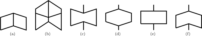

    

    Front views of cells of $3D$-periodic structures

  • cell ${\mathcal{S}}$ of Fig. 1(c)

    $$ \hbox{dim}({\mathbb{M}}_{s}({\mathcal{S}}))=5,\quad {\mathbb{V}}_{\varGamma}(\varOmega ,{\mathcal{S}})=\Big\{ {\mathcal{U}}\in H^{1}_{\varGamma}( \varOmega )^{3}\; |\; {\frac{\partial {\mathcal{U}}_{1}}{\partial x_{1}}}=0 \quad \hbox{a.e. in }\; \varOmega \Big\} , $$

    the matrix $\mathfrak {B}^{hom}$ is of size $5\times 5$.

• 2. Type $\mathbb{S}_{1}$:

  • cell ${\mathcal{S}}$ of Fig. 1(d)

    $$ \hbox{dim}({\mathbb{M}}_{s}({\mathcal{S}}))=3,\quad {\mathbb{V}}_{\varGamma}(\varOmega ,{\mathcal{S}})=\Big\{ {\mathcal{U}}\in H^{1}_{\varGamma}( \varOmega )^{3}\; |\; {\frac{\partial {\mathcal{U}}_{1}}{\partial x_{1}}}={ \frac{\partial {\mathcal{U}}_{2}}{\partial x_{2}}}={ \frac{\partial {\mathcal{U}}_{3}}{\partial x_{3}}}=0\ \ \, \hbox{a.e. in }\; \varOmega \Big\} , $$

    the matrix $\mathfrak {B}^{hom}$ is of size $3\times 3$,

  • cell ${\mathcal{S}}$ of Fig. 1(e)

    $$\begin{aligned} &\hbox{dim}({\mathbb{M}}_{s}({\mathcal{S}}))=4,\\ &\quad {\mathbb{V}}_{\varGamma}(\varOmega ,{\mathcal{S}})=\Big\{ {\mathcal{U}}\in H^{1}_{\varGamma}( \varOmega )^{3}\; |\; {\frac{\partial {\mathcal{U}}_{2}}{\partial x_{2}}}= \kappa _{12}{\frac{\partial {\mathcal{U}}_{1}}{\partial x_{1}}}, \quad {\frac{\partial {\mathcal{U}}_{3}}{\partial x_{3}}}=\kappa _{13}{ \frac{\partial {\mathcal{U}}_{1}}{\partial x_{1}}}, \quad \hbox{a.e. in }\; \varOmega \Big\} , \end{aligned}$$

    where $\kappa _{12}<0$ and $\kappa _{13}<0$. These coefficients depend on the slopes of the oblique segments and their signs mean that the Poisson’s ratios in planes parallel to ${\mathbb{R}}{\mathbf{e}}_{1}\oplus {\mathbb{R}}{\mathbf{e}}_{2}$ and ${\mathbb{R}}{\mathbf{e}}_{1}\oplus {\mathbb{R}}{\mathbf{e}}_{3}$ are positive. We also get

    $$ {\frac{\partial {\mathcal{U}}_{3}}{\partial x_{3}}}={ \frac{\kappa _{13}}{\kappa _{12}}}{ \frac{\partial {\mathcal{U}}_{2}}{\partial x_{2}}}, \quad \hbox{a.e. in }\; \varOmega . $$

    This relation means that the structure is auxetic in planes parallel to ${\mathbb{R}}{\mathbf{e}}_{2}\oplus {\mathbb{R}}{\mathbf{e}}_{3}$. The matrix $\mathfrak {B}^{hom}$ is of size $4\times 4$,

  • cell ${\mathcal{S}}$ of Fig. 1(f)

    $$\begin{aligned} &\hbox{dim}({\mathbb{M}}_{s}({\mathcal{S}}))=4,\\ &\quad {\mathbb{V}}_{\varGamma}(\varOmega ,{\mathcal{S}})=\Big\{ {\mathcal{U}}\in H^{1}_{\varGamma}( \varOmega )^{3}\; |\; {\frac{\partial {\mathcal{U}}_{2}}{\partial x_{2}}}= \kappa _{12}{\frac{\partial {\mathcal{U}}_{1}}{\partial x_{1}}}, \quad {\frac{\partial {\mathcal{U}}_{3}}{\partial x_{3}}}=\kappa _{13}{ \frac{\partial {\mathcal{U}}_{1}}{\partial x_{1}}}, \quad \hbox{a.e. in }\; \varOmega \Big\} , \end{aligned}$$

    where $\kappa _{12}>0$ and $\kappa _{13}>0$. These coefficients depend on the slopes of the oblique segments and their signs mean that the Poisson’s ratios in planes parallel to ${\mathbb{R}}{\mathbf{e}}_{1}\oplus {\mathbb{R}}{\mathbf{e}}_{2}$, ${\mathbb{R}}{\mathbf{e}}_{1}\oplus {\mathbb{R}}{\mathbf{e}}_{3}$ and ${\mathbb{R}}{\mathbf{e}}_{2}\oplus {\mathbb{R}}{\mathbf{e}}_{3}$ are negative, the matrix $\mathfrak {B}^{hom}$ is of size $4\times 4$. This structure is completely auxetic,

  • cell ${\mathcal{S}}$ of Fig. 5(f) in planes parallel to ${\mathbb{R}}{\mathbf{e}}_{1}\oplus {\mathbb{R}}{\mathbf{e}}_{2}$ and ${\mathbb{R}}{\mathbf{e}}_{1}\oplus {\mathbb{R}}{\mathbf{e}}_{3}$

    $$ \hbox{dim}({\mathbb{M}}_{s}({\mathcal{S}}))=5,\quad {\mathbb{V}}_{\varGamma}(\varOmega ,{\mathcal{S}})=\Big\{ {\mathcal{U}}\in H^{1}_{\varGamma}( \varOmega )^{3}\; |\; {\frac{\partial {\mathcal{U}}_{1}}{\partial x_{1}}}=0 \quad \hbox{a.e. in }\; \varOmega \Big\} , $$

    the matrix $\mathfrak {B}^{hom}$ is of size $5\times 5$.

• 3. Type $\mathbb{S}_{2}$:

  • the cell ${\mathcal{S}}$ is such that in planes parallel to ${\mathbb{R}}{\mathbf{e}}_{1}\oplus {\mathbb{R}}{\mathbf{e}}_{2}$ we get only non convex hexagons like Fig. 5(c)

    $$ \hbox{dim}({\mathbb{M}}_{s}({\mathcal{S}}))=5,\quad {\mathbb{V}}_{\varGamma}(\varOmega ,{\mathcal{S}})=\Big\{ {\mathcal{U}}\in H^{1}_{\varGamma}( \varOmega )^{3}\; |\; {\frac{\partial {\mathcal{U}}_{2}}{\partial x_{2}}}= \kappa _{12}{\frac{\partial {\mathcal{U}}_{1}}{\partial x_{1}}} \quad \hbox{a.e. in }\; \varOmega \Big\} , $$

    where $\kappa _{12}>0$. This coefficient depends on the slopes of the oblique segments, the matrix $\mathfrak {B}^{hom}$ is of size $5\times 5$.

14.3 Concluding Remark Concerning the Mechanical Impact

We recall the solution procedure, to compute the cell problems and find the homogenized elastic coefficients.

First, as explained in Sect. 3, we determine the conditions for which equation (3.1) admits solutions. This gives ${\mathbb{M}}_{s}({\mathcal{S}})$ and then a basis $\big\{\mathfrak {M}_{p},\;\; i=1,\ldots ,P\big\}$. The knowledge of ${\mathbb{M}}_{s}({\mathcal{S}})$ takes into account the relations between the matrices $\mathbf{M}_{11}$, $\mathbf{M}_{22}$, $\mathbf{M}_{33}$ and of course the $\kappa _{ij}$ if they are defined.

After that we get $\widehat {{\mathcal{B}}}_{V}(\mathfrak {M}_{p})$, $p\in \{1,\ldots ,P\}$; we modify them in order to have $\widehat {{\mathcal{B}}}(\mathfrak {M}_{p})$, $p\in \{1,\ldots ,P\}$ and then use them to solve (12.7) by means of the Galerkin method, using (A.4) as test functions.

We also want to draw the attention on the mechanical impact of the paper. Since we want to stay in the linear elasticity regime, we need to choose forces, such that the right-hand side functional is bounded in the same order, as the elastic energy. In [19], we gave the order of each single loading component, i.e., the externally applied nodal forces $F(A)$, the moments $G(A)$, and the constant in the cross-section axial expansion forces, $\mathbf{f}_{|{\mathcal{S}}_{\varepsilon }}$, in the set of beams $\displaystyle \bigcup _{\xi \in \varXi _{\varepsilon }} \bigcup _{\ell =1}^{m} {\mathcal{P}}^{\xi}_{\varepsilon ,\ell ,r}$, that does not violate the linear elasticity for the stable structures. This scaling is the following:

$$ f_{\varepsilon }= \sum _{A\in {\mathcal{K}}_{\varepsilon }}\Big[{ \frac{\varepsilon ^{2}}{r^{2}}}F(A)+{\frac{\varepsilon }{r^{3}}}G(A) \land (x-A)\Big]{\mathbf{1}}_{B(A,r)} +{ \frac{\varepsilon }{r+\varepsilon ^{2}}}{\mathbf{f}}_{|{\mathcal{S}}_{ \varepsilon }}{\mathbf{1}}_{\cup _{\xi \in \varXi _{\varepsilon }}\cup _{ \ell =1}^{m}{\mathcal{P}}_{\varepsilon \ell ,r}^{\xi}}, $$

(14.1)

where $(\mathbf{f},\,F,\,G)\in \big(C(\overline{\varOmega })^{3}\big)^{3}$ and $\mathbf{1}_{{\mathcal{O}}}$ is the characteristic function of the set ${\mathcal{O}}$. This scaling realizes

$$ \Big|\int _{{\mathcal{S}}_{\varepsilon ,r}}f_{\varepsilon }\cdot u\,dx \Big|\leq C\big(\|{\mathbf{f}}\|_{L^{\infty}(\varOmega )}+\|F\|_{L^{\infty}( \varOmega )}+\|G\|_{L^{\infty}(\varOmega )}\big)\|e(u)\|_{L^{2}({\mathcal{S}}_{ \varepsilon ,r})},\quad \forall \, u\in {\mathbf{V}}_{\varepsilon ,r}. $$

(14.2)

For the unstable structures, applied forces should be smaller to realize a linear elastic regime in the structure of thin beams,

$$ \Big|\int _{{\mathcal{S}}_{\varepsilon ,r}}f_{\varepsilon }\cdot u\,dx \Big|\leq C{\frac{r^{2}}{\varepsilon ^{2}}}\big(\|{\mathbf{f}}\|_{L^{\infty}(\varOmega )}+\|{\mathbf{F}}\|_{L^{\infty}(\varOmega )}+\|{\mathbf{G}}\|_{L^{\infty}(\varOmega )}\big)\|e(u)\|_{L^{2}({\mathcal{S}}_{\varepsilon ,r})}, \qquad \forall u\in {\mathbf{V}}_{\varepsilon ,r}. $$

(14.3)

This requires the following component scaling:

$$ f_{\varepsilon }\doteq \sum _{A\in {\mathcal{K}}_{\varepsilon }}\Big[{ \frac{r}{\varepsilon }}{\mathbf{F}}(A)+{\frac{1}{r\varepsilon }}{\mathbf{G}}(A) \land (x-A)\Big]{\mathbf{1}}_{B(A,r)} +{\frac{r^{2}}{\varepsilon ^{2}}}{ \mathbf {f}}_{|{\mathcal{S}}_{\varepsilon }}. $$

(14.4)

In Examples in Sect. 14.2 of this paper, we mean “locking” under the applied loading range. However, the unstable structures with long zig-zag lines, mentioned as “locked” in a certain direction in Sect. 14.2, are stable for the loading in this direction and so, the axial forces on beams can be chosen larger in their projection to this direction. I.e., for the structure of type $\mathbb{S}_{0}$ axial forces can be chosen as

$$ \widetilde{\mathbf{f}}_{\varepsilon }={\frac{r}{\varepsilon }} \big( \widetilde{f}_{1}{\mathbf{1}}_{\varOmega ^{(1)}_{\varepsilon }}\big)_{|{ \mathcal{S}}^{(1)}_{\varepsilon }}\,\mathbf{e}_{1},\qquad \widetilde{f}_{1} \in {\mathcal{C}}(\overline{\varOmega ^{(1)}}), $$

without changing the estimate below ((6.7) in this paper),

$$ \|e(u_{\varepsilon })\|_{L^{2}({\mathcal{S}}_{\varepsilon ,r})}\le C{ \frac{r^{2}}{\varepsilon ^{2}}}\big(\|{\mathbf{f}}\|_{L^{\infty}(\varOmega )}+ \|{\mathbf{F}}\|_{L^{\infty}(\varOmega )}+\|{\mathbf{G}}\|_{L^{\infty}(\varOmega )} \big). $$

(14.5)

This criteria on the applied forces, can be used to design structures, i.e., to find a correct proportion between $r$ and $\varepsilon$, in order to stay in the linear elastic regime under certain required loading.

Appendix

Lemma 26

Let ${\mathcal{S}}$ be a $3D$-periodic structure of type $\mathbb{S}_{i}$. If ${\mathcal{S}}$ contains at least a straight line of direction $\mathbf{e}_{i}$, $i\in \{1,2,3\}$, then a necessary condition to solve (3.1) is

$$ {\mathbf{M}}_{ii}=0. $$

(A.1)

Proof

Let $V$ be a solution to (3.1). Since $V$ is periodic, integrating along a straight line of direction $\mathbf{e}_{i}$ leads to $\mathbf{M}_{ii}=0$. The condition (A.1) is required. □

Lemma 27

Let ${\mathcal{S}}$ be a structure of type $\mathbb{S}_{i}$, $i\in \{0,1,2,5\}$. Then, a sufficient condition to solve (3.1) is

$$ {\mathbf{M}}_{11}=\mathbf{M}_{22}=\mathbf{M}_{33}=0. $$

(A.2)

Proof

Let $\mathbf{M}$ be a matrix satisfying (A.2). We define $\mathbf{W}\in {\mathbf{U}}_{per}({\mathcal{S}})$ by

$$ \mathbf{W}({\mathbf{S}})=-2\widehat{\mathbf{e}_{1}}({\mathbf{S}})\,\mathbf{M}\,\mathbf{e}_{1}+{ \mathbf {C}},\qquad \forall {\mathbf{S}}\in {\mathcal{S}},\qquad \mathbf{C}\in { \mathbb{R}}^{3}. $$

The derivative of $\mathbf{W}$ is

$$ {\frac{d\mathbf{W}}{d{\mathbf{S}}}}=-2\big(\mathbf{e}_{1}\cdot {\mathbf{t}}_{1} \big)\mathbf{M}\, \mathbf{e}_{1}\qquad \hbox{a.e. in } \;\;{\mathcal{S}}. $$

Hence, due to assumption (A.2)

$$ {\frac{d\mathbf{W}}{d{\mathbf{S}}}}\cdot {\mathbf{t}}_{1}=-2\big(\mathbf{e}_{1} \cdot {\mathbf{t}}_{1}\big)\big(\mathbf{M}\, \mathbf{e}_{1}\big)\cdot {\mathbf{t}}_{1}=- \big(\mathbf{M}\,\mathbf{t}_{1}\big)\cdot {\mathbf{t}}_{1}\qquad \hbox{a.e. in } \enskip {\mathcal{S}}. $$

We project $\mathbf{W}$ over $\mathbf{D}_{E,per}({\mathcal{S}})$ which gives $V(\mathbf{M})$, the solution to (3.1). □

Denote ${\mathbb{M}}_{S,3}$ the space of $3\times 3$ symmetric matrices.

One can prove the following lemma:

Lemma 28

Let ${\mathcal{S}}$ be a structure of type $\mathbb{S}_{j}$, $j\in \{0,1,2\}$. There exist linear forms $L_{i,{\mathcal{S}}}: \; {\mathbb{M}}_{S,3}\to {\mathbb{R}}$ and functions $g_{i}\in H^{1}_{per}({\mathcal{S}})$ satisfying

$$ {\frac{d g_{i}}{d{\mathbf{S}}}}=0\qquad \hbox{a.e. in } \; {\mathcal{S}}^{(i)}, \;\; i\in \{1,2,3\} $$

such that for every $\mathbf{M}\in {\mathbb{M}}_{S,3}$ the following problem admits a unique solution:

$$ \mathbf{W}(\mathbf{M})\in {\mathbf{D}}_{E,per}({\mathcal{S}}),\qquad { \frac{d\mathbf{W}(\mathbf{M})}{d{\mathbf{S}}}}\cdot {\mathbf{t}}_{1}=-(\mathbf{M}\,{ \mathbf {t}}_{1})\cdot {\mathbf{t}}_{1}+L_{i,{\mathcal{S}}}(\mathbf{M})g_{i}\;\; \hbox{ on }\;\; {\mathcal{S}}^{(i)}, \;\; i\in \{1,2,3\}. $$

For every matrix $\mathbf{M}\in {\mathbb{M}}_{S,3}$, we have:

if ${\mathcal{S}}$ is of type

• $\mathbb{S}_{0}$ then $L_{1,{\mathcal{S}}}(\mathbf{M})=\mathbf{M}_{11}$,

• $\mathbb{S}_{1}$ then $L_{1,{\mathcal{S}}}(\mathbf{M})=0$,

• $\mathbb{S}_{2}$ then $L_{1,{\mathcal{S}}}(\mathbf{M}) =L_{2,{\mathcal{S}}}(\mathbf{M})=0$.

Hence

$$ {\mathbb{M}}_{s}({\mathcal{S}})=\big\{ \mathbf{M}\in {\mathbb{M}}_{S,3}\;| \; L_{1,{\mathcal{S}}}(\mathbf{M})= L_{2,{\mathcal{S}}}(\mathbf{M})= L_{3,{ \mathcal{S}}}(\mathbf{M})=0\,\big\} . $$

As a consequence of the above lemma, regarding the dimension of ${\mathbb{M}}_{s}({\mathcal{S}})$, one has:

• if ${\mathcal{S}}$ is of type $\mathbb{S}_{0}$ then $\hbox{dim}\big({\mathbb{M}}_{s}({\mathcal{S}})\big)\in \{3,4,5\}$, all the dimensions are possible,

• if ${\mathcal{S}}$ is of type $\mathbb{S}_{1}$ then $\hbox{dim}\big({\mathbb{M}}_{s}({\mathcal{S}})\big)\in \{3,4,5,6\}$, in this case it would seem that $\hbox{dim}\big({\mathbb{M}}_{s}({\mathcal{S}})\big)=6$ is not possible,

• if ${\mathcal{S}}$ is of type $\mathbb{S}_{2}$ then $\hbox{dim}\big({\mathbb{M}}_{s}({\mathcal{S}})\big)\in \{5,6\}$.

1.1 A.1 The Warping-Correctors

The four warping-correctors are the solutions to the following cell problems:

$$ \begin{aligned} & \hskip 1cm \widetilde{\chi}_{E}({\mathbf{S}},\cdot )\in {\boldsymbol{{\mathcal{D}}}}_{w},\; \; \widetilde{\chi}_{q}({\mathbf{S}},\cdot )\in {\boldsymbol{{\mathcal{D}}}}_{w}, \;\; q\in \{1,2,3\}, \\ &\int _{D} a_{ijkl}({\mathbf{S}})\,\big({\mathcal{E}}_{D}( \widetilde{\chi}_{E})({\mathbf{S}},\cdot )+\mathbf{M}^{11}\big)_{ij}\big({ \mathcal{E}}_{D}(\widetilde{v})\big)_{kl}\,dS_{2}dS_{3}=0, \\ &\int _{D} a_{ijkl}({\mathbf{S}})\,\big({\mathcal{E}}_{D}( \widetilde{\chi}_{1})({\mathbf{S}},\cdot )+{S_{2}}{\mathbf{M}}^{13}-{S_{3}}{ \mathbf {M}}^{12}\big)_{ij}\big({\mathcal{E}}_{D}(\widetilde{v})\big)_{kl} \,dS_{2}dS_{3}=0, \\ &\int _{D} a_{ijkl}({\mathbf{S}})\,\big({\mathcal{E}}_{D}( \widetilde{\chi}_{2})({\mathbf{S}},\cdot )+S_{3}{\mathbf{M}}^{11}\big)_{ij} \big({\mathcal{E}}_{D}(\widetilde{v})\big)_{kl}\,dS_{2}dS_{3}=0, \\ &\int _{D} a_{ijkl}({\mathbf{S}})\,\big({\mathcal{E}}_{D}( \widetilde{\chi}_{3})({\mathbf{S}},\cdot )-S_{2}{\mathbf{M}}^{11}\big)_{ij} \big({\mathcal{E}}_{D}(\widetilde{v})\big)_{kl}\,dS_{2}dS_{3}=0, \end{aligned} \qquad \begin{aligned}&\hbox{for a.e. ${\mathbf{S}}$ in }{\mathcal{S}},\\ &\forall \, \widetilde{v}\in {\boldsymbol{{\mathcal{D}}}}_{w}. \end{aligned} $$

(A.3)

We easily obtain

$$ \begin{aligned} \widetilde{\chi}_{E}=-{ \frac{E_{12}E_{33}-E_{13}E_{23}}{E_{22}E_{33}-E_{23}^{2}}}S_{2}{\mathbf{t}}_{2}+{ \frac{E_{12}E_{23}-E_{13}E_{22}}{E_{22}E_{33}-E_{23}^{2}}}S_{3}{\mathbf{t}}_{3}, \qquad \widetilde{\chi}_{1}=\chi _{T}{\mathbf{t}}_{1}, \end{aligned} $$

where $\chi _{T}\in L^{\infty}({\mathcal{S}}; H^{1}(D))$ is the solution to the variational problem

$$\begin{aligned} &\int _{D}\chi _{T}\,dS_{2}dS_{3}=0,\\ & \int _{D} G_{12}\Big({ \frac{\partial \chi _{T}}{\partial S_{2}}}-S_{3}\Big){ \frac{\partial \phi }{\partial S_{2}}}+G_{13}\Big({ \frac{\partial \chi _{T}}{\partial S_{3}}}+S_{2}\Big){ \frac{\partial \phi }{\partial S_{3}}}dS_{2}dS_{3}=0,\qquad \forall \phi \in H^{1}(D). \end{aligned}$$

The correctors $\widetilde{\chi}_{i}\in L^{\infty}({\mathcal{S}}; H^{1}(D))^{3}$, $i\in \{2,3\}$ are the solutions to

$$ \begin{aligned} &\widetilde{\chi}_{i1}=0,\qquad \int _{D}\big(S_{3}\widetilde{\chi}_{i2}-S_{2} \widetilde{\chi}_{i3}\big)dS_{2}dS_{3}=\int _{D}\widetilde{\chi}_{i}dS_{2}dS_{3}=0, \\ &\int _{D}\Big[\Big(E_{12}S_{3}+ E_{22}{ \frac{\partial \widetilde{\chi}_{22}}{\partial S_{2}}}+ E_{23}{ \frac{\partial \widetilde{\chi}_{23}}{\partial S_{3}}}\Big){ \frac{\partial \phi _{2}}{\partial S_{2}}}+\Big(E_{13}S_{3}+ E_{23}{ \frac{\partial \widetilde{\chi}_{22}}{\partial S_{2}}}+ E_{33}{ \frac{\partial \widetilde{\chi}_{23}}{\partial S_{3}}}\Big){ \frac{\partial \phi _{3}}{\partial S_{3}}} \\ &\qquad \quad +{\frac{G_{23}}{4}}\Big({ \frac{\partial \widetilde{\chi}_{22}}{\partial S_{3}}}+{ \frac{\partial \widetilde{\chi}_{23}}{\partial S_{2}}}\Big)\Big({ \frac{\partial \phi _{2}}{\partial S_{3}}}+{ \frac{\partial \phi _{3}}{\partial S_{2}}}\Big)\Big]dS_{2}dS_{3}=0 \qquad \forall (\phi _{2},\phi _{3})\in H^{1}(D)^{2}, \\ &\int _{D}\Big[\Big(-E_{12}S_{2}+ E_{22}{ \frac{\partial \widetilde{\chi}_{32}}{\partial S_{2}}}+ E_{23}{ \frac{\partial \widetilde{\chi}_{33}}{\partial S_{3}}}\Big){ \frac{\partial \phi _{2}}{\partial S_{2}}}+\Big(-E_{13}S_{2}+ E_{23}{ \frac{\partial \widetilde{\chi}_{32}}{\partial S_{2}}}+ E_{33}{ \frac{\partial \widetilde{\chi}_{33}}{\partial S_{3}}}\Big){ \frac{\partial \phi _{3}}{\partial S_{3}}} \\ &\qquad \quad +{\frac{G_{23}}{4}}\Big({ \frac{\partial \widetilde{\chi}_{32}}{\partial S_{3}}}+{ \frac{\partial \widetilde{\chi}_{33}}{\partial S_{2}}}\Big)\Big({ \frac{\partial \phi _{2}}{\partial S_{3}}}+{ \frac{\partial \phi _{3}}{\partial S_{2}}}\Big)\Big]dS_{2}dS_{3}=0 \qquad \forall (\phi _{2},\phi _{3})\in H^{1}(D)^{2}. \end{aligned} $$

Observe that due to the symmetries of $D$,

$$ \widetilde{\chi}_{22},\;\;\widetilde{\chi}_{33}\;\; \hbox{are odd with respect to $S_{2}$ and $S_{3}$},\quad \widetilde{\chi}_{23},\;\; \widetilde{\chi}_{32}\;\; \hbox{are even with respect to $S_{2}$ and $S_{3}$}. $$

1.2 A.2 The Spaces $\mathbf{D}_{I,per}({\mathcal{S}})$, $\boldsymbol{\mathcal {D}}_{I,per}({\mathcal{S}})$ and $\mathfrak {D}_{I,per}({\mathcal{S}})$

Let ${\mathcal{A}}$ be an inextensional displacement belonging to $\mathbf{D}_{I,per}({\mathcal{S}})$. There exists ${\mathcal{B}}\in L^{\infty}({\mathcal{S}})$ constant on every segment of ${\mathcal{S}}$ and satisfying ${\mathcal{B}}\cdot {\mathbf{t}}_{1}=0$ a.e. on ${\mathcal{S}}$ such that

$$ {\frac{d {\mathcal{A}}}{d{\mathbf{S}}}}= {\mathcal{B}}\land {\mathbf{t}}_{1} \quad \hbox{a.e. in} \;\; {\mathcal{S}}. $$

Proceeding in the same way as to build the couple $\big(\widehat {{\mathcal{A}}}(\mathbf{M}),\,\widehat {{\mathcal{B}}}({ \mathbf {M}})\big)$, we obtain $\big(\widetilde {{\mathcal{A}}},\,\widetilde {{\mathcal{B}}}\big) \in \boldsymbol{\mathcal {D}}_{I,per}({\mathcal{S}})$ such that

$$ \begin{aligned} &\widetilde {{\mathcal{A}}}={\mathcal{A}}\quad \hbox{and}\quad \widetilde {{\mathcal{B}}}=0\quad \hbox{on every node of ${\mathcal{S}}$ and} \\ &\hbox{on every segment $\gamma \subset {\mathcal{S}}$}\;\; \widetilde{{\mathcal{B}}}_{|\gamma}\; \hbox{is a polynomial function of degree less than 2}. \end{aligned} $$

The map ${\mathcal{A}}\in {\mathbf{D}}_{I,per}({\mathcal{S}})\longrightarrow \big( \widetilde {{\mathcal{A}}},\,\widetilde {{\mathcal{B}}}\big)\in \boldsymbol{\mathcal {D}}_{I,per}({\mathcal{S}})$ is one to one.

Now, let ℬ be in $\mathbf{U}_{per}({\mathcal{S}})$. We recall the following result: Let $\psi$ be a function affine on $[a,b]$, $a< b$. Then function $\widetilde{\psi}$ defined by

$$ \begin{aligned} &\widetilde{\psi}(t)= \psi (a){\frac{b-t}{b-a}}+\psi (b){ \frac{t-a}{b-a}}+ 3\big(\psi (a)+\psi (b)\big){ \frac{(t-a)(t-b)}{(b-a)^{2}}} \quad \hbox{in}\;\; [a,b], \\ &\hbox{satisfies}\;\; \int _{a}^{b}\widetilde{\psi}(t)dt=0,\qquad \widetilde{\psi}(a)=\psi (a),\;\; \widetilde{\psi}(b)=\psi (b). \end{aligned} $$

(A.4)

With the help of this function, we build a couple $\big(\overline{{\mathcal{A}}},\,\overline{{\mathcal{B}}}\big)\in \boldsymbol{\mathcal {D}}_{I,per}({\mathcal{S}})$ such that¹⁴

$$ \begin{aligned} &\overline{{\mathcal{A}}}=0\quad \hbox{and}\quad \overline{{\mathcal{B}}}={\mathcal{B}}\quad \hbox{on every node of ${\mathcal{S}}$ and } \\ \ &\hbox{on every segment $\gamma \subset {\mathcal{S}}$,}\;\; \overline{{\mathcal{B}}}_{|\gamma}\; \hbox{is a polynomial function of degree less than 2.} \end{aligned} $$

The map ${\mathcal{B}}\in {\mathbf{U}}_{per}({\mathcal{S}})\longrightarrow \big( \overline{{\mathcal{A}}},\,\overline{{\mathcal{B}}}\big)\in \boldsymbol{\mathcal {D}}_{I,per}({\mathcal{S}})$ is one to one.

Denote $\mathfrak {D}_{I,per}({\mathcal{S}})$ the subspace of $\boldsymbol{\mathcal {D}}_{I,per}({\mathcal{S}})$ containing the sums $\big(\widetilde {{\mathcal{A}}},\,\widetilde {{\mathcal{B}}}\big)+ \big(\overline{{\mathcal{A}}},\,\overline{{\mathcal{B}}}\big)$. This space is isomorphic to $\mathbf{D}_{I,per}({\mathcal{S}})\times \mathbf{U}_{per}({\mathcal{S}})$.

1.3 A.3 The Test Function $\phi ^{[1]}_{\varepsilon ,r}$

To every $\phi$ in $H^{1}({\mathcal{S}}_{\varepsilon })$, we associate the function $\phi ^{[1]}_{\varepsilon ,r}$ defined by:

• $\phi ^{[1]}_{\varepsilon ,r}$ is constant in the neighborhood of every node,

• in the segment $[\varepsilon \xi +\varepsilon A^{\ell}-c_{0} r\mathbf{t}^{\ell}_{1}, \varepsilon \xi +\varepsilon B^{\ell}+c_{0}r\mathbf{t}^{\ell}_{1}]$, $\gamma _{\ell}=[A^{\ell},B^{\ell}]$, $\xi \in \varXi _{\varepsilon }$, $\gamma _{\ell}\subset {\mathcal{S}}$

  $$ \phi ^{[1]}_{\varepsilon ,r}(\mathbf{s})= \left \{ \begin{aligned} &\phi \big(\varepsilon \xi +\varepsilon A^{\ell}\big)\qquad && \hbox{for all } s_{1}\in [-c_{0}r,c_{0} r], \\ &\hbox{polynomial function of degree less than 1 } \;&& \hbox{for all } s_{1} \in [c_{0} r , \varepsilon l_{\ell}-c_{0} r], \\ &\phi \big(\varepsilon \xi +\varepsilon B^{\ell}\big)\quad && \hbox{for all } s_{1}\in [\varepsilon l_{\ell}-c_{0} r, \varepsilon l_{\ell}+c_{0}r] \end{aligned} \right . $$

  where the polynomial function is defined for all $s_{1}\in [c_{0} r , \varepsilon l_{\ell}-c_{0} r]$ by

  $$ \phi ^{[1]}_{\varepsilon ,r}(\mathbf{s})=\phi \big(\varepsilon \xi + \varepsilon A^{\ell}\big){ \frac{\varepsilon l_{\ell}-c_{0}r-s_{1}}{\varepsilon l_{\ell}-2c_{0}r}}+ \phi \big(\varepsilon \xi +\varepsilon B^{\ell}\big){ \frac{s_{1}-c_{0}r}{\varepsilon l_{\ell}-2c_{0}r }}. $$

  $\phi ^{[1]}_{\varepsilon ,r}$ belongs to $W^{1,\infty}(\varepsilon \xi +\varepsilon A^{\ell}-c_{0} r\mathbf{t}^{\ell}_{1}, \varepsilon \xi +\varepsilon B^{\ell}+c_{0} r\mathbf{t}^{\ell}_{1})$.

In that way, we obtain a function belonging to $W^{1,\infty}({\mathcal{S}}_{\varepsilon })$, constant in the neighborhood of every node. That allows to extend it as an element, still denoted $\phi ^{[1]}_{\varepsilon ,r}$, belonging to $W^{1,\infty}({\mathcal{S}}_{\varepsilon ,r})$, constant in every domain $B(\varepsilon \xi +\varepsilon A, c_{0} r)\cap {\mathcal{S}}_{ \varepsilon ,r}$, $A\in {\mathcal{K}}$, and also constant in every cross-section of the beams. This function satisfies

$$ \begin{aligned} &{\frac{d\phi ^{[1]}_{\varepsilon ,r}}{d\mathbf{s}}}(\mathbf{s})={ \frac{\phi \big(\varepsilon \xi +\varepsilon B^{\ell}\big)-\phi \big(\varepsilon \xi +\varepsilon A^{\ell}\big)}{\varepsilon l_{\ell}-2c_{0}r}} \quad \hbox{for all } s_{1}\in [c_{0} r , \varepsilon l_{\ell}-c_{0} r], \\ &\big\| \phi ^{[1]}_{\varepsilon ,r}- \phi \big\| _{L^{2}({\mathcal{S}}_{ \varepsilon })}\leq C\varepsilon \Big\| {\frac{d\phi }{d\mathbf{s}}} \Big\| _{L^{2}({\mathcal{S}}_{\varepsilon })},\qquad \Big\| { \frac{d\phi ^{[1]}_{\varepsilon ,r}}{d\mathbf{s}}}\Big\| _{L^{2}({ \mathcal{S}}_{\varepsilon })}\leq C\Big\| {\frac{d\phi }{d\mathbf{s}}} \Big\| _{L^{2}({\mathcal{S}}_{\varepsilon })}. \end{aligned} $$

(A.5)

The constant does not depend on $\varepsilon$ and $r$. Moreover, if $\phi$ belongs to $W^{1,\infty}(\varOmega )$, one has

$$ \begin{aligned} {\mathcal{T}}^{\mathcal{S}}_{\varepsilon}\big(\phi ^{[1]}_{ \varepsilon ,r}\big) & \longrightarrow \phi \quad \hbox{strongly in } L^{2}( \varOmega \times {\mathcal{S}}), \\ {\mathcal{T}}^{\mathcal{S}}_{\varepsilon}\Big({ \frac{d\phi ^{[1]}_{\varepsilon ,r}}{d\mathbf{s}}}\Big) & \longrightarrow \nabla \phi \cdot {\mathbf{t}}_{1} \quad \hbox{strongly in } L^{2}(\varOmega \times {\mathcal{S}}). \end{aligned} $$

(A.6)

1.4 A.4 The Test Function $\phi ^{[2]}_{\varepsilon }$

To every $\phi$ in $H^{1}({\mathcal{S}}_{\varepsilon })$, we associate the function $\phi ^{[2]}_{\varepsilon }$ defined by:

• $\phi ^{[2]}_{\varepsilon }$ is constant in the neighborhood of every node,

• in the segment $[\varepsilon \xi +\varepsilon A^{\ell}-c_{0} r\mathbf{t}^{\ell}_{1}, \varepsilon \xi +\varepsilon B^{\ell}+c_{0}r\mathbf{t}^{\ell}_{1}]$, $\gamma _{\ell}=[A^{\ell},B^{\ell}]$, $\xi \in \varXi _{\varepsilon }$, $\gamma _{\ell}\subset {\mathcal{S}}$

  $$ \phi ^{[2]}_{\varepsilon }(\mathbf{s})= \left \{ \begin{aligned} &\phi \big(\varepsilon \xi +\varepsilon A^{\ell}\big)\qquad && \hbox{for all } s_{1}\in [-c_{0}r,c_{0} r], \\ &\hbox{polynomial function of degree less than 3 } \;&& \hbox{for all } s_{1} \in [c_{0} r , \varepsilon l_{\ell}-c_{0} r], \\ &\phi \big(\varepsilon \xi +\varepsilon B^{\ell}\big)\quad && \hbox{for all } s_{1}\in [\varepsilon l_{\ell}-c_{0} r, \varepsilon l_{\ell}+c_{0}r], \end{aligned} \right . $$

  where the polynomial function is defined for all $s_{1}\in [c_{0} r , \varepsilon l_{\ell}-c_{0} r]$ by

  $$\begin{aligned} \phi ^{[2]}_{\varepsilon }(\mathbf{s})&=\phi \big(\varepsilon \xi + \varepsilon A^{\ell}\big){ \frac{(s_{1}-\varepsilon l_{\ell}+c_{0}r)^{2}(\varepsilon l_{\ell}-4c_{0}r+2s_{1})}{(\varepsilon l_{\ell}-2c_{0}r)^{3}}}\\ &\quad+ \phi \big(\varepsilon \xi +\varepsilon B^{\ell}\big){ \frac{(s_{1}-c_{0}r)^{2}(3\varepsilon l_{\ell}-4c_{0}r- 2s_{1})}{(\varepsilon l_{\ell}-2c_{0}r)^{3}}}. \end{aligned}$$

  $\phi ^{[2]}_{\varepsilon }$ belongs to $W^{2,\infty}(\varepsilon \xi +\varepsilon A^{\ell}-c_{0} r\mathbf{t}^{\ell}_{1}, \varepsilon \xi +\varepsilon B^{\ell}+c_{0} r\mathbf{t}^{\ell}_{1})$.

In that way, we obtain a function belonging to $W^{1,\infty}({\mathcal{S}}_{\varepsilon })$, constant in the neighborhood of every node. That allows to extend it as an element, still denoted $\phi ^{[2]}_{\varepsilon }$, belonging to $W^{1,\infty}({\mathcal{S}}_{\varepsilon ,r})$, constant in every domain $B(\varepsilon \xi +\varepsilon A, c_{0} r)\cap {\mathcal{S}}_{ \varepsilon ,r}$, $A\in {\mathcal{K}}$, and also constant in every cross-section of the beams. This function satisfies

$$ \begin{aligned} &{\frac{d\phi ^{[2]}_{\varepsilon }}{d\mathbf{s}}}(\mathbf{s})={ \frac{\phi \big(\varepsilon \xi +\varepsilon B^{\ell}\big)-\phi \big(\varepsilon \xi +\varepsilon A^{\ell}\big)}{\varepsilon l_{\ell}-2c_{0}r}}{ \frac{6(s_{1}-c_{0}r)(\varepsilon l_{\ell}-c_{0}r-s_{1})}{(\varepsilon l_{\ell}-2c_{0}r)^{2}}} \\ &\quad \hbox{for all } s_{1}\in [c_{0} r , \varepsilon l_{\ell}-c_{0} r], \\ &\big\| \phi ^{[2]}_{\varepsilon }- \phi \big\| _{L^{2}({\mathcal{S}}_{ \varepsilon })}\leq C\varepsilon \Big\| {\frac{d\phi }{d\mathbf{s}}} \Big\| _{L^{2}({\mathcal{S}}_{\varepsilon })},\qquad \Big\| { \frac{d\phi ^{[2]}_{\varepsilon }}{d\mathbf{s}}}\Big\| _{L^{2}({ \mathcal{S}}_{\varepsilon })}\leq C\Big\| {\frac{d\phi }{d\mathbf{s}}} \Big\| _{L^{2}({\mathcal{S}}_{\varepsilon })}, \\ & \Big\| {\frac{d^{2}\phi ^{[2]}_{\varepsilon }}{d\mathbf{s}^{2}}} \Big\| _{L^{2}({ \mathcal{S}}_{\varepsilon })}\leq {\frac{C}{\varepsilon }}\Big\| { \frac{d\phi }{d\mathbf{s}}}\Big\| _{L^{2}({\mathcal{S}}_{\varepsilon })}. \end{aligned} $$

(A.7)

The constant does not depend on $\varepsilon$ and $r$. Moreover, if $\phi$ belongs to $W^{1,\infty}(\varOmega )$, one has

$$ \begin{aligned} {\mathcal{T}}^{\mathcal{S}}_{\varepsilon}\big(\phi ^{[2]}_{ \varepsilon }\big) & \longrightarrow \phi \quad \hbox{strongly in } L^{2}( \varOmega \times {\mathcal{S}}), \\ {\mathcal{T}}^{\mathcal{S}}_{\varepsilon}\Big({ \frac{d\phi ^{[2]}_{\varepsilon }}{d\mathbf{s}}}\Big) & \longrightarrow \nabla \phi \cdot {\mathbf{t}}_{1}{\boldsymbol{\varPhi}}\quad \hbox{strongly in } L^{2}( \varOmega \times {\mathcal{S}}), \\ \varepsilon {\mathcal{T}}^{\mathcal{S}}_{\varepsilon}\Big({ \frac{d^{2}\phi ^{[2]}_{\varepsilon }}{d\mathbf{s}^{2}}}\Big) & \longrightarrow \nabla \phi \cdot {\mathbf{t}}_{1}{ \frac{d{\boldsymbol{\varPhi}}}{d{\mathbf{S}}}}\quad \hbox{strongly in } L^{2}(\varOmega \times {\mathcal{S}}), \end{aligned} $$

(A.8)

where ${\boldsymbol{\varPhi}}$ belongs to $H^{1}_{0,{\mathcal{K}}}({\mathcal{S}})$ and in $\gamma _{\ell}\subset {\mathcal{S}}$ it is defined by

$$ {\boldsymbol{\varPhi}}({\mathbf{S}})={\frac{S_{1}(l_{\ell}-S_{1})}{l^{2}_{\ell}}}\quad \hbox{for all } S_{1}\in [0,l_{\ell}]. $$

(A.9)

1.5 A.5 The Test Function $\phi ^{[3]}_{\varepsilon }$

To every $\phi$ in $W^{2,\infty}({\mathbb{R}}^{3})$, we associate the function $\phi ^{[3]}_{\varepsilon }\in W^{2,\infty}({\mathcal{S}}_{ \varepsilon })$ defined by:

• $\phi ^{[3]}_{\varepsilon }$ is affine in the neighborhood of every node,

• for $\mathbf{s}=\varepsilon \xi + \varepsilon A^{\ell}+s_{1}{\mathbf{t}}^{\ell}_{1}$, $s_{1}\in [-c_{0}r,\varepsilon l_{\ell}+c_{0}r]$, $\gamma _{\ell}=[A^{\ell},B^{\ell}]$, $\xi \in \varXi _{\varepsilon }$, $\gamma _{\ell}\subset {\mathcal{S}}$, we set

$$ \phi ^{[3]}_{\varepsilon }(\mathbf{s})= \left \{ \begin{aligned} &\phi \big(\varepsilon \xi +\varepsilon A^{\ell}\big)+s_{1}\nabla \phi \big(\varepsilon \xi +\varepsilon A^{\ell}\big)\cdot {\mathbf{t}}^{\ell}_{1}\quad && \hbox{for all } s_{1}\in [-c_{0} r, c_{0}r], \\ &\hbox{see (A.10) } && \hbox{for all } s_{1}\in [c_{0} r , 2c_{0}r ] , \\ &\phi (\mathbf{s})\qquad && \hbox{for all } s_{1}\in [2c_{0} r , \varepsilon l_{\ell}- 2c_{0}r ] , \\ &\hbox{ see (A.10) } && \hbox{for all } s_{1}\in [\varepsilon l_{\ell}-2c_{0} r , \varepsilon l_{\ell}-c_{0}r ] , \\ &\phi \big(\varepsilon \xi +\varepsilon B^{\ell}\big)+(s_{1}- \varepsilon l_{\ell})\nabla \phi \big(\varepsilon \xi +\varepsilon B^{\ell}\big)\cdot {\mathbf{t}}^{\ell}_{1} && \hbox{for all } s_{1}\in [ \varepsilon l_{\ell}-c_{0} r ,\varepsilon l_{\ell}+ c_{0}r ], \end{aligned} \right . $$

where for all $s_{1}\in [c_{0} r , 2c_{0} r]$

$$ \begin{aligned} \phi ^{[3]}_{\varepsilon }(\mathbf{s})=&\big( \phi \big(\varepsilon \xi + \varepsilon A^{\ell}\big)+c_{0}r \nabla \phi \big(\varepsilon \xi + \varepsilon A^{\ell}\big)\cdot {\mathbf{t}}^{\ell}_{1}\big){ \frac{(s_{1}-2c_{0}r)^{2}\big(2(s_{1}-c_{0}r)+c_{0}r\big)}{(c_{0}r)^{3}}} \\ &+\nabla \phi \big(\varepsilon \xi +\varepsilon A^{\ell}\big)\cdot { \mathbf {t}}^{\ell}_{1}{ \frac{(s_{1}-2c_{0}r)^{2}(s_{1}-c_{0}r)}{(c_{0}r)^{2}}} \\ &+\phi \big(\varepsilon \xi +\varepsilon A^{\ell}+2c_{0} r\mathbf{t}^{\ell}_{1}\big){ \frac{(s_{1}-c_{0}r)^{2}\big(-2(s_{1}-2c_{0}r)+c_{0}r\big)}{(c_{0}r)^{3}}} \\ &+\nabla \phi \big(\varepsilon \xi +\varepsilon A^{\ell}+2c_{0} r\mathbf{t}^{\ell}_{1}\big)\cdot {\mathbf{t}}^{\ell}_{1}{ \frac{(s_{1}-c_{0}r)^{2}(s_{1}-2c_{0}r)}{(c_{0}r)^{2}}}. \end{aligned} $$

(A.10)

We easily check that

$$ {\frac{d\phi ^{[3]}_{\varepsilon }}{d\mathbf{s}}}(\mathbf{s})= \left \{ \begin{aligned} &\nabla \phi \big(\varepsilon \xi +\varepsilon A^{\ell}\big)\cdot { \mathbf {t}}^{\ell}_{1}\quad && \hbox{for all } s_{1}\in [-c_{0} r, c_{0}r] , \\ &\hbox{see (A.11)} && \hbox{for all } s_{1}\in [c_{0} r , 2c_{0}r ] , \\ &\nabla \phi (\mathbf{s})\cdot {\mathbf{t}}^{\ell}_{1}\qquad && \hbox{for all } s_{1} \in [2c_{0} r ,\varepsilon l_{\ell}- 2c_{0}r ] , \\ &\hbox{ see (A.11) } && \hbox{for all } s_{1}\in [\varepsilon l_{\ell}-2c_{0} r , \varepsilon l_{\ell}-c_{0}r ] , \\ &\nabla \phi \big(\varepsilon \xi +\varepsilon B^{\ell}\big)\cdot { \mathbf {t}}^{\ell}_{1}\quad && \hbox{for all } s_{1}\in [\varepsilon l_{\ell}-c_{0} r ,\varepsilon l_{\ell}+ c_{0}r ], \end{aligned} \right . $$

where for all $s_{1}\in [\varepsilon l_{\ell}-2c_{0} r , \varepsilon l_{\ell}-c_{0}r ]$

$$ \begin{aligned} {\frac{d\phi ^{[3]}_{\varepsilon }}{d\mathbf{s}}}(\mathbf{s})=&\Big(\phi \big(\varepsilon \xi +\varepsilon A^{\ell}\big)+c_{0} r\nabla \phi \big(\varepsilon \xi +\varepsilon A^{\ell}\big)\cdot {\mathbf{t}}^{\ell}_{1}- \phi \big(\varepsilon \xi +\varepsilon A^{\ell}+2c_{0} r\mathbf{t}^{\ell}_{1} \big) \\ &+{\frac{c_{0}r}{2}}\big[\nabla \phi \big(\varepsilon \xi + \varepsilon A^{\ell}\big)+\nabla \phi \big(\varepsilon \xi + \varepsilon A^{\ell}+2c_{0} r\mathbf{t}^{\ell}_{1}\big)\big]\cdot {\mathbf{t}}^{\ell}_{1}\Big){\frac{6(s_{1}-2c_{0}r)(s_{1}-c_{0}r)}{(c_{0}r)^{3}}} \\ &+\nabla \phi \big(\varepsilon \xi +\varepsilon A^{\ell}+2c_{0} r\mathbf{t}^{\ell}_{1}\big)\cdot {\mathbf{t}}^{\ell}_{1}{\frac{ s_{1}-c_{0}r}{c_{0}r}}- \nabla \phi \big(\varepsilon \xi +\varepsilon A^{\ell}\big)\cdot {\mathbf{t}}^{\ell}_{1}{\frac{s_{1}-2c_{0}r }{c_{0}r}}. \end{aligned} $$

(A.11)

The function $\phi ^{[3]}_{\varepsilon }$ satisfies

$$ \big\| \phi ^{[3]}_{\varepsilon }- \phi \big\| _{L^{\infty}({\mathcal{S}}_{ \varepsilon })}\leq C r^{2} \| \phi \|_{W^{2,\infty}({\mathbb{R}}^{3})}, \quad \Big\| {\frac{d\phi ^{[3]}_{\varepsilon }}{d\mathbf{s}}}- \nabla \phi \cdot {\mathbf{t}}_{1}\Big\| _{L^{\infty}({\mathcal{S}}_{\varepsilon })} \leq C r \| \phi \|_{W^{2,\infty}({\mathbb{R}}^{3})}. $$

(A.12)

The constant does not depend on $\varepsilon$ and $r$.

1.6 A.6 A Lemma of the Periodic Unfolding Method

Denote

$$ \begin{aligned} {\mathbf{A}}_{\varGamma}({\mathcal{S}})&\doteq \Big\{ \varPhi \in H^{1}_{\varGamma}({ \mathcal{S}}_{\varepsilon })\;|\; \varPhi \; \hbox{ is an affine function on every segment}\Big\} , \\ \mathbf{A}_{per}({\mathcal{S}})&\doteq \Big\{ \varPhi \in H^{1}_{per}({ \mathcal{S}})\;|\; \varPhi \; \hbox{ is an affine function on every segment} \Big\} , \\ H^{1}_{0,{\mathcal{K}}_{\varepsilon }}({\mathcal{S}}_{\varepsilon })& \doteq \Big\{ \phi \in H^{1}({\mathcal{S}}_{\varepsilon })\;|\; \phi \; \hbox{vanishes on every node}\;\Big\} . \end{aligned} $$

Lemma 29

Let ${\mathcal{S}}$ be a $3D$-periodic structure of type $\mathbb{S}_{i}$, $i\in \{0,1,2\}$ and $\{\phi _{\varepsilon }\}_{\varepsilon }$ a sequence of functions belonging to $H^{1}_{\varGamma}({\mathcal{S}}_{\varepsilon })$, satisfying

$$ \|\phi _{\varepsilon }\|_{L^{2}({\mathcal{S}}_{\varepsilon })}+ \Big\| {\frac{d\phi _{\varepsilon }}{d\mathbf{s}}}\Big\| _{L^{2}({ \mathcal{S}}^{(3)}_{\varepsilon })}+ {\varepsilon }\sum _{i =1}^{2} \Big\| {\frac{d\phi _{\varepsilon }}{d\mathbf{s}}}\Big\| _{L^{2}({ \mathcal{S}}^{(i )}_{\varepsilon })}\leq {\frac{C}{\varepsilon }}. $$

Then, up to a subsequence still denoted $\{\varepsilon \}$, there exist $\widetilde{\phi }\in L^{2}_{\varGamma}(\varOmega ,\partial _{3},{ \mathcal{S}})$ and $\widehat{\phi }\in L^{2}(\varOmega ; H^{1}_{per}({\mathcal{S}}))$ such that ($i \in \{1,2\}$)

$$ \begin{aligned} & {\mathcal{T}}^{\mathcal{S}}_{\varepsilon}\big(\phi _{\varepsilon } \big)\rightharpoonup \widetilde{\phi }\quad \textit{ weakly in} \quad L^{2}( \varOmega ; H^{1}({\mathcal{S}})), \\ &\varepsilon {\mathcal{T}}^{\mathcal{S}}_{\varepsilon}\Big({ \frac{d\phi _{\varepsilon }}{d\mathbf{s}}}\Big)\rightharpoonup { \frac{\partial \widetilde{\phi }}{\partial {\mathbf{S}}}}\quad \textit{ weakly in} \quad L^{2}(\varOmega \times {\mathcal{S}}^{(i )}), \\ &{\mathcal{T}}^{\mathcal{S}}_{\varepsilon}\Big({ \frac{d\phi _{\varepsilon }}{d\mathbf{s}}}\Big)\rightharpoonup { \frac{\partial \widetilde{\phi }}{\partial x_{3}}}+{ \frac{\partial \widehat{\phi }}{\partial {\mathbf{S}}}}\quad \textit{ weakly in} \quad L^{2}(\varOmega \times {\mathcal{S}}^{(3)}).\end{aligned} $$

(A.13)

Proof

Step 1. We decompose $\phi _{\varepsilon }$ as

$$ \phi _{\varepsilon }=\phi ^{a}_{\varepsilon }+\phi ^{0}_{\varepsilon }, \qquad \phi ^{a}_{\varepsilon }\in {\mathbf{A}}_{\varGamma}({\mathcal{S}}_{ \varepsilon }),\qquad \phi ^{0}_{\varepsilon }\in H^{1}_{0,{ \mathcal{K}}_{\varepsilon }}({\mathcal{S}}_{\varepsilon }). $$

The assumptions on $\{\phi _{\varepsilon }\}_{\varepsilon }$ imply that

$$ \begin{aligned} &\|\phi ^{a}_{\varepsilon }\|_{L^{2}({\mathcal{S}}_{\varepsilon })}+ \Big\| {\frac{d\phi ^{a}_{\varepsilon }}{d\mathbf{s}}}\Big\| _{L^{2}({ \mathcal{S}}^{(3)}_{\varepsilon })}+ {\varepsilon }\sum _{i =1}^{2} \Big\| {\frac{d\phi ^{a}_{\varepsilon }}{d\mathbf{s}}}\Big\| _{L^{2}({ \mathcal{S}}^{(i )}_{\varepsilon })}\leq {\frac{C}{\varepsilon }}, \\ & {\frac{1}{\varepsilon }}\|\phi ^{0}_{\varepsilon }\|_{L^{2}({ \mathcal{S}}^{(3)}_{\varepsilon })}+ \Big\| { \frac{d\phi ^{0}_{\varepsilon }}{d\mathbf{s}}}\Big\| _{L^{2}({\mathcal{S}}^{(3)}_{ \varepsilon })}+ \sum _{i =1}^{2}\Big(\|\phi ^{0}_{\varepsilon }\|_{L^{2}({ \mathcal{S}}^{(i)}_{\varepsilon })}+\varepsilon \Big\| { \frac{d\phi ^{0}_{\varepsilon }}{d\mathbf{s}}}\Big\| _{L^{2}({\mathcal{S}}^{(i )}_{\varepsilon })}\Big)\leq {\frac{C}{\varepsilon }}. \end{aligned} $$

Then, up to a subsequence still denoted $\{\varepsilon \}$, there exists $\widetilde{\phi ^{0}}\in L^{2}(\varOmega ; H^{1}_{0,{\mathcal{K}}}({ \mathcal{S}}^{(i)}))$ (see (10.1)) such that

$$ \begin{aligned} {\mathcal{T}}^{\mathcal{S}}_{\varepsilon}\big(\phi ^{0}_{\varepsilon } \big) & \rightharpoonup \widetilde{\phi ^{0}}\quad \text{ weakly in} \quad L^{2}(\varOmega ; H^{1}_{0,{\mathcal{K}}}({\mathcal{S}}^{(i)})),\; \; i\in \{1,2\}, \\ {\frac{1}{\varepsilon }}{\mathcal{T}}^{\mathcal{S}}_{\varepsilon}\big( \phi ^{0}_{\varepsilon }\big) & \rightharpoonup \widetilde{\phi ^{0}} \quad \text{ weakly in} \quad L^{2}(\varOmega ; H^{1}_{0,{\mathcal{K}}}({ \mathcal{S}}^{(3)})), \\ \varepsilon {\mathcal{T}}^{\mathcal{S}}_{\varepsilon}\Big({ \frac{d\phi ^{0}_{\varepsilon }}{d\mathbf{s}}}\Big) & \rightharpoonup { \frac{\partial \widetilde{\phi ^{0}}}{\partial {\mathbf{S}}}}\quad \text{ weakly in} \quad L^{2}(\varOmega \times {\mathcal{S}}^{(i)}),\;\; i \in \{1,2\}, \\ {\mathcal{T}}^{\mathcal{S}}_{\varepsilon}\Big({ \frac{d\phi ^{0}_{\varepsilon }}{d\mathbf{s}}}\Big) & \rightharpoonup { \frac{\partial \widetilde{\phi ^{0}}}{\partial {\mathbf{S}}}}\quad \text{ weakly in} \quad L^{2}(\varOmega \times {\mathcal{S}}^{(3)}). \end{aligned} $$

Step 2. Limit of the sequence $\big\{{\mathcal{T}}^{\mathcal{S}}_{\varepsilon}(\phi ^{a}_{ \varepsilon })\big\}_{\varepsilon }$.

The assumptions on $\{\phi _{\varepsilon }\}_{\varepsilon }$ imply that

$$ \|\phi ^{a}_{\varepsilon }\|_{L^{2}({\mathcal{S}}_{\varepsilon })}+ \varepsilon \Big\| {\frac{d\phi ^{a}_{\varepsilon }}{d\mathbf{s}}}\Big\| _{L^{2}({ \mathcal{S}}_{\varepsilon })}\leq {\frac{C}{\varepsilon }}. $$

Then, up to a subsequence still denoted $\{\varepsilon \}$, there exists $\widetilde{\phi ^{a}}\in L^{2}(\varOmega ; \mathbf{A}_{per}({\mathcal{S}}))$ such that

$$ \begin{aligned} {\mathcal{T}}^{\mathcal{S}}_{\varepsilon}\big(\phi ^{a}_{\varepsilon } \big) & \rightharpoonup \widetilde{\phi ^{a}}\quad \text{ weakly in} \quad L^{2}(\varOmega ; H^{1}({\mathcal{S}})), \\ \varepsilon {\mathcal{T}}^{\mathcal{S}}_{\varepsilon}\Big({ \frac{d\phi ^{a}_{\varepsilon }}{d\mathbf{s}}}\Big) & \rightharpoonup { \frac{\partial \widetilde{\phi ^{a}}}{\partial {\mathbf{S}}}}\quad \text{ weakly in} \quad L^{2}(\varOmega \times {\mathcal{S}}). \end{aligned} $$

(A.14)

Hence

$$ \varepsilon {\mathcal{T}}^{\mathcal{S}}_{\varepsilon}\Big({ \frac{d\phi _{\varepsilon }}{d\mathbf{s}}}\Big) \rightharpoonup { \frac{\partial (\widetilde{\phi ^{0}}+\widetilde{\phi ^{a}})}{\partial {\mathbf{S}}}} \quad \text{ weakly in} \quad L^{2}(\varOmega \times {\mathcal{S}}^{(i)}), \quad i\in \{1,2\}. $$

Since $\displaystyle \varepsilon \Big\|{ \frac{d\phi ^{a}_{\varepsilon }}{d\mathbf{s}}}\Big\|_{L^{2}({\mathcal{S}}^{(3)}_{ \varepsilon })}\leq C$, we have $\partial _{{\mathbf{S}}}\,\widetilde{\phi ^{a}}=0$ a.e. on $\varOmega \times {\mathcal{S}}^{(3)}$.

Step 3. Limit of the sequence $\displaystyle \Big\{{\mathcal{T}}^{\mathcal{S}}_{\varepsilon}\Big({ \frac{d\phi _{\varepsilon }}{d\mathbf{s}}}\Big)\Big\}_{\varepsilon }$ in $L^{2}(\varOmega \times {\mathcal{S}}^{(3)})$.

We decompose the restriction of $\phi ^{a}_{\varepsilon }$ to the zig-zag lines of ${\mathcal{S}}^{(3)}_{\varepsilon }$ as

$$ \phi ^{a}_{\varepsilon }=\varPhi ^{a}_{\varepsilon }+\varPsi ^{a}_{ \varepsilon }, $$

where $\displaystyle {\frac{d\varPhi ^{a}_{\varepsilon }}{d\mathbf{s}}}$ is constant on every zig-zag line in $\varepsilon \xi +\varepsilon {\mathcal{S}}^{(3)}$ and where $\varPsi ^{a}_{\varepsilon }$ vanishes on all the extremities of the zig-zag lines in $\varepsilon \xi +\varepsilon {\mathcal{S}}^{(3)}$. One has

$$ \|\varPhi ^{a}_{\varepsilon }\|_{L^{2}({\mathcal{S}}^{(3)}_{\varepsilon })}+ \Big\| {\frac{d\varPhi ^{a}_{\varepsilon } }{d\mathbf{s}}}\Big\| _{L^{2}({ \mathcal{S}}^{(3)}_{\varepsilon })}+\varepsilon \|\varPsi ^{a}_{ \varepsilon }\|_{L^{2}({\mathcal{S}}^{(3)}_{\varepsilon })}+ \Big\| { \frac{d\varPsi ^{a}_{\varepsilon } }{d\mathbf{s}}}\Big\| _{L^{2}({ \mathcal{S}}^{(3)}_{\varepsilon })}\leq {\frac{C}{\varepsilon }}. $$

Then, up to a subsequence still denoted $\{\varepsilon \}$, there exist $\varPhi ^{a}\in L^{2}_{\varGamma}(\varOmega ,\partial _{3},{\mathcal{S}})$ and $\widehat{\phi ^{a}}\in L^{2}(\varOmega ; \mathbf{A}_{per}({\mathcal{S}}^{(3)}))$ (see (2.5)₅) extended in a function belonging to $L^{2}(\varOmega ; \mathbf{A}_{per}({\mathcal{S}}))$ still denoted $\widehat{\phi ^{a}}$ such that (see [12, Lemma 6.8])

$$ \begin{aligned} & {\mathcal{T}}^{\mathcal{S}}_{\varepsilon}\big(\varPhi ^{a}_{ \varepsilon }\big)\rightharpoonup \varPhi ^{a}=\widetilde{\phi ^{a}} \quad \text{ weakly in} \quad L^{2}(\varOmega ; H^{1}({\mathcal{S}}^{(3)})), \\ &{\mathcal{T}}^{\mathcal{S}}_{\varepsilon}\Big({ \frac{d\varPhi ^{a}_{\varepsilon }}{d\mathbf{s}}}\Big)\rightharpoonup { \frac{\partial \varPhi ^{a}}{\partial x_{3}}}\quad \text{ weakly in} \quad L^{2}(\varOmega \times {\mathcal{S}}^{(3)}), \\ {\frac{1}{\varepsilon }}&{\mathcal{T}}^{\mathcal{S}}_{\varepsilon}\Big(\varPsi ^{a}_{\varepsilon }\Big)\rightharpoonup \widehat{\phi ^{a}} \quad \text{ weakly in} \quad L^{2}(\varOmega ; H^{1}({\mathcal{S}}^{(3)})). \end{aligned} $$

This ends the proof of the lemma setting $\widetilde{\phi }=\widetilde{\phi ^{0}}+\widetilde{\phi ^{a}}$ a.e. in $\varOmega \times {\mathcal{S}}^{(i)}$, $i\in \{1,2\}$, $\widetilde{\phi }=\widetilde{\phi ^{a}}$ a.e. in $\varOmega \times {\mathcal{S}}^{(3)}$ and $\widehat{\phi }=\widetilde{\phi ^{0}}+\widehat{\phi ^{a}}$ a.e. in $\varOmega \times {\mathcal{S}}^{(3)}$. □

References

Abdoul-Anziz, H., Seppecher, P., Bellis, C.: Homogenization of frame lattices leading to second gradient models coupling classical strain and strain-gradient terms. Math. Mech. Solids 24(12), 3976–3999 (2019)
Antman, S.S.: The theory of rods. In: Függe, S., Truesdell, C. (eds.) Handbuch der Physik, pp. 641–703. Springer, Berlin (1972)
Askesa, H., Aifantis, E.C.: Gradient elasticity in statics and dynamics: an overview of formulations, length scale identification procedures, finite element implementations and new results. Int. J. Solids Struct. 48, 1962–1990 (2011)
Blanchard, D., Griso, G.: Asymptotic behavior of structures made of straight rods. J. Elast. 108(1), 85–118 (2012)
Blanchard, D., Gaudiello, A., Griso, G.: Junction of a periodic family of elastic rods with a 3d plate. Part I. J. Math. Pures Appl. 88(1), 1–33 (2007)
Casado-Díaz, J., Luna-Laynez, M., Martín, J.D., Gómez, J.D.: Homogenization of very thin elastic reticulated structures. J. Mech. Behav. Mater. 16(4–5), 297–304 (2005)
Ciarlet, P.G.: Mathematical Elasticity II: Lower-Dimensional Theories of Plates and Rods. North-Holland, Amsterdam (1990)
Cioranescu, D., Saint Jean Paulin, J.: Homogenization of Reticulated Structures. Applied Mathematical Sciences, vol. 136. Springer, New York (1999)
Cioranescu, D., Damlamian, A., Griso, G.: Periodic unfolding and homogenization. C. R. Math. 335(1), 99–104 (2002)
Cioranescu, D., Damlamian, A., Griso, G.: The periodic unfolding method in homogenization. SIAM J. Math. Anal. 40(4), 1585–1620 (2008)
Cioranescu, D., Damlamian, A., Griso, G.: The Periodic Unfolding Method: Theory and Applications to Partial Differential Problems. Springer, Berlin (2018)
Falconi, R., Griso, G., Orlik, J.: Anisotropic extension of the unfolding tools (2021, submitted)
Griso, G.: Asymptotic behavior of curved rods by the unfolding method. Math. Methods Appl. Sci. 27(17), 2081–2110 (2004)
Griso, G.: Asymptotic behavior of structures made of curved rods. Anal. Appl. 6(1), 11–22 (2008)
Griso, G.: Decompositions of displacements of thin structures. J. Math. Pures Appl. 89, 199–223 (2008)
Griso, G., Miara, B.: Homogenization of periodically heterogeneous thin beams. Chin. Ann. Math., Ser. B 39(3), 397–426 (2018)
Griso, G., Orlik, J.: Homogenization of contact problem with Coulomb’s friction on periodic cracks. Math. Methods Appl. Sci. 42(18), 6435–6458 (2019)
Griso, G., Migunova, A., Orlik, J.: Asymptotic analysis for domains separated by a thin layer made of periodic vertical beams. J. Elast. 128(2), 291–331 (2017)
Griso, G., Khilkova, L., Orlik, J., Sivak, O.: Homogenization of perforated elastic structures. J. Elast. 141, 181–225 (2020). https://doi.org/10.1007/s10659-020-09781
Griso, G., Orlik, J., Wackerle, S.: Asymptotic behavior for textiles in von-Kármán regime. J. Math. Pures Appl. 144, 164–193 (2020)
Griso, G., Orlik, J., Wackerle, S.: Homogenization of textiles. SIAM J. Math. Anal. 52(2), 1639–1689 (2020)
Griso, G., Hauck, M., Orlik, J.: Asymptotic analysis for periodic perforated shells. ESAIM: M2AN (2021). https://doi.org/10.1051/m2an/2020067
Griso, G., Khilkova, L., Orlik, J., Sivak, O.: Asymptotic behavior of stable structures made of beams. J. Elast. (2021). https://doi.org/10.1007/s10659-021-09816-w
Kolzlov, V., Maz’ya, V., Mocvchan, A.: Asymptotic Analysis of Fields in Multi-Structures. Clarendon Press, Oxford (1999)
Lakes, R.S.: Physical meaning of elastic constants in Cosserat, void, and microstretch elasticity. J. Mech. Mater. Struct. 11(3), 217–229 (2016)
Landau, L.D., Lifshitz, E.M.: In: Sykes, J.B., Bell, J.S. (eds.) Mechanics, 3rd edn. Course of Theoretical Physics, vol. 1. Pergamon, Oxford (1976). ISBN 0-08-021022-8. OCLC 2591126
Le Dret, H.: Modelling of the junction between two rods. J. Math. Pures Appl. 68(3), 365–397 (1989)
Le Dret, H.: Problèmes variationnels dans les multi-domaines. Modélisation des jonctions et applications. Elsevier, Amsterdam (1991)
Liu, G.R., Quek, S.S.: The Finite Element Method: A Practical Course. Butterworth, Stoneham (2013)
Martinsson, P.G., Babuška, I.: Homogenization of materials with periodic truss or frame micro-structures. Math. Models Methods Appl. Sci. 17(5), 805–832 (2007)
Orlik, J., Panasenko, G., Shiryaev, V.: Optimization of textile-like materials via homogenization and dimension reduction. Multiscale Model. Simul. 14(2), 637–667 (2016)
Panasenko, G.: Asymptotic solutions of the system of elasticity theory for rod and frame structures. Russ. Acad. Sci., Math. Sb. 75(1), 85–110 (1993)
Pastukhova, S.: Homogenization of problems of elasticity theory on periodic box and rod frames of critical thickness. J. Math. Sci. 130, 4954–5004 (2005)
Pilkey, W.: Analysis and Design of Elastic Beams. Computational Methods. Wiley, New York (2002)
Trabucho, L., Viano, J.M.: Mathematical Modelling of Rods. Handbook of Numerical Analysis, vol. 4. North-Holland, Amsterdam (1996)
Zhikov, V., Pastukhova, S.: Homogenization for elasticity problems on periodic networks of critical thickness. Sb. Math. 194(5), 61–96 (2003)
Acknowledgements
The authors would like to thank Viacheslav Khilkov for his help in the development and construction of \(3D\)-structures.
Funding
Open Access funding enabled and organized by Projekt DEAL.
Author information
Authors and Affiliations
Corresponding author
Additional information
Publisher’s Note
Springer Nature remains neutral with regard to jurisdictional claims in published maps and institutional affiliations.