An experimental evaluation of Siamese Neural Networks for robot localization using omnidirectional imaging in indoor environments

Abstract

The objective of this paper is to address the localization problem using omnidirectional images captured by a catadioptric vision system mounted on the robot. For this purpose, we explore the potential of Siamese Neural Networks for modeling indoor environments using panoramic images as the unique source of information. Siamese Neural Networks are characterized by their ability to generate a similarity function between two input data, in this case, between two panoramic images. In this study, Siamese Neural Networks composed of two Convolutional Neural Networks (CNNs) are used. The output of each CNN is a descriptor which is used to characterize each image. The dissimilarity of the images is computed by measuring the distance between these descriptors. This fact makes Siamese Neural Networks particularly suitable to perform image retrieval tasks. First, we evaluate an initial task strongly related to localization that consists in detecting whether two images have been captured in the same or in different rooms. Next, we assess Siamese Neural Networks in the context of a global localization problem. The results outperform previous techniques for solving the localization task using the COLD-Freiburg dataset, in a variety of lighting conditions, specially when using images captured in cloudy and night conditions.

1 Introduction

During the past few years, vision sensors have been used extensively in the field of map building and localization with mobile robots (Hu et al. 2020; Zhong et al. 2018). In particular, the ability to localize in the map is of paramount importance in order to develop autonomous robots that can navigate in real operating conditions. The interest in using vision sensors to capture information from the environment is still high. Cameras can capture a big amount of information from the environment with a relatively low cost and they can be used in both, indoor and outdoor areas. Additionally, the images permit carrying out other highly specialized tasks such as object recognition and people detection.

Among the available configurations to capture visual information, the use of omnidirectional vision sensors in mobile robotics has become common. Omnidirectional cameras obtain images that cover a field of view of 360° around the robot (Junior et al. 2016). As a result, they are commonly used to address navigation tasks (Rituerto et al. 2010).

The large amount of information provided by cameras requires robust techniques to extract and describe the relevant visual information. Different paradigms have been considered to extract this relevant information. A first group of techniques concentrate on detecting, describing and tracking some landmarks or local features along the scenes (Cao et al. 2020; Lin et al. 2020). Different local features have been used in mapping and localization tasks, including SIFT, SURF and ORB descriptors (E. Rublee and Bradski 2011). A global description of each image can then be obtained, for example, by means of the Bag of Words model (Raúl Mur-Artal and Tardós 2015). A second group of techniques work with each scene as a whole, and build a unique descriptor per image that contains information on its global appearance (Korrapati and Mezouar 2017; Khaliq et al. 2019). Finally, hardware developments have led many authors to use Artificial Intelligence (AI) techniques to extract relevant information from images. Specifically, Convolutional Neural Networks (CNNs) have been proposed to address different computer vision and robotics tasks. For example, Xu et al. (2019) and Leyva-Vallina et al. (2019) proposed global appearance descriptors based on a CNN to obtain the most probable pose of the robot.

In general terms, holistic description methods lead to maps in which a set of robot poses and their associated descriptors are stored. In this way, each pose of the robot is represented by a holistic descriptor and this representation leads to straightforward localization algorithms, based on the pairwise comparison between descriptors.

In this manuscript we assess the usage of Siamese Neural Networks in the context of image description and robot localization. Siamese Neural Networks permit evaluating two images at the same time in such a way that they provide a similarity measurement at the output. Therefore, they have the potential to address visual recognition of places and estimate the position of a mobile robot. In the present paper, we evaluate this potential. The main contributions of this paper can be summarized as follows.

• 1. We explore the capability of Siamese Neural Networks for modeling indoor environments, using panoramic images as the unique source of information.

• 2. We train and evaluate Siamese Neural Networks with the purpose of detecting whether two images have been captured in the same or in different rooms.

• 3. We train Siamese Neural Networks capable of estimating robot position as a global image retrieval problem.

• 4. We conduct an exhaustive study on the influence of the Siamese Neural Networks’ architecture and the most relevant parameters. Moreover, we analyze the robustness against some common visual phenomena that may occur in real operating conditions, such as changes of the lighting conditions or image blur.

The following sections are structured as follows. First, in Sect. 2 we present a review of the state of the art on visual localization and mapping using Artificial Intelligence techniques. Second, in Sect. 3 we introduce Siamese Neural Networks for both room discrimination and global localization. After that, Sect. 4 presents the CNN architectures, the dataset and the proposed data augmentation. Furthermore, in this section we also describe the proposed method for room discrimination and global localization by means of Siamese Neural Networks. Then, Sect. 5 describes the experiments carried out to test and validate the proposed method. Finally, conclusions and future works are outlined in Sect. 6.

2 State of the art

As stated before, Siamese Neural Networks are able to generate a similarity function from pairs of input data. They can be regarded as a superstructure that includes two Neural Networks. These architectures accept two different inputs and offer a single output. The underlying networks share the same weights and different functions can be used to conform a single output. They were first proposed in 1993 in order to distinguish correct signatures from forgeries (Bromley et al. 1993). Since then, these architectures have been proposed in different areas of knowledge. For example, Thiolliere et al. (2015) proposed a Siamese Neural Network for audio and speech signal processing, Zheng et al. (2019) used this architecture for the comparison of DNA sequences or Jeon et al. (2019) used it for drug discovery purposes. Furthermore, Parajuli et al. (2017) developed a Siamese Neural Network to track cardiac motion and Sandouk and Chen (2017) proposed a Siamese architecture in order to recognize music tags. Recently, Suljagic et al. (2022) use this kind of architecture for multi-object tracking (MOT) and person re-identification.

During the past few years, AI in general and CNNs in particular have been used in the field of mobile robotics for a variety of purposes. For instance, for mapping (Sinha et al. 2018; Moolan-Feroze et al. 2019), localization (Weinzaepfel et al. 2019; Cattaneo et al. 2019), navigation (Zhao et al. 2018; Ma et al. 2019) and simultaneous localization and mapping (Lu and Lu 2019; Liu et al. 2019). A complete state-of-the-art review on mobile robotics tasks based on the use of AI can be found in (Cebollada et al. 2020). Other applications of AI in the context of mobile robotics include: self-driving navigation (Polvara et al. 2018; Organisciak et al. 2020), face detection and recognition (Wang et al. 2017; Hu et al. 2021), object recognition and categorization (Zaki et al. 2019; Feng et al. 2020) and mapping and localization (Holliday and Dudek 2018; Ruan et al. 2019).

Convolutional Neural Networks (CNNs) are the most popular techniques among AI tools. Currently, they are used in many mapping and localization tasks due to their successful performance in many practical applications. They are designed to receive images as input and their structures are specially created to obtain descriptors that synthesize the information in them (Chollet et al. 2018). Therefore, they can be used to describe the global appearance of an image. In this sense, Cebollada et al. (2019) proposed holistic descriptors obtained with a CNN to perform localization within topological models, studying their strength against illumination variations. Also, Xu et al. (2019) and Leyva-Vallina et al. (2019) proposed these techniques to obtain the most probable robot position. Additionally, Ballesta et al. (2021) studied localization tasks using CNNs and regression layers as global appearance descriptors. Recently, Rostkowska and Skrzypczyński (2023) employed the EfficientNet model (Tan and Le 2019) to embed an omnidirectional image into a single descriptor followed by a K-Nearest Neighbours (KNN) algorithm to robustly predict the topological position in a given database (map). In this regard, this work implements the Facebook AI Similarity Search (FAISS) library (Johnson et al. 2019) to efficiently perform the nearest neighbour search using a KD-Tree.

Some well known architectures have been used as basic structures to develop new modified networks for robotic navigation purposes. AlexNet (Krizhevsky et al. 2012), VGG16 (Simonyan and Zisserman 2014), GoogleNet (Szegedy et al. 2015) or NetVLAD (Arandjelovic et al. 2016) are some of them.

The Convolutional Neural Networks presented above can be used to form a Siamese Neural Network. In the field of robotics, they have been rarely used and some studies that proposed this structure in this field are mentioned below. For example, Utkin et al. (2017) use a Siamese Neural Network to support the security control of a robot by detecting anomalies in its behaviour and Zeng et al. (2018) present a robotic pick-and-place system capable of identifying and grasping both known and novel objects in cluttered environments using a Siamese Neural Network. Moreover, Li and Zhang (2019) use the VGG16 network to conform a Siamese structure for object detection and tracking. Additionally, Zhang and Peng (2019) presented a study in which Siamese Networks are followed by Fully Connected layers or Region Proposal Network structures in the context of real-time visual tracking.

Regarding robot localization tasks, Leyva-Vallina et al. have proposed the use of Siamese Neural Networks to address the place recognition problem in garden environments (Leyva-Vallina et al. 2019, 2021). Moreover, this architecture has been proposed for localization using LiDAR scans (Yin et al. 2018; Chen et al. 2022).

In the present paper, we address the localization of a mobile robot using panoramic images in such a way that we study in detail different architectures and training configurations of Siamese Neural Networks. For this purpose, we propose as an initial approach to train and test the capability of the network to distinguish between images captured in the same and different rooms. In addition, in this study we also tackle the global localization problem using Siamese Neural Networks.

3 Visual localization using Siamese Neural Networks

Siamese Neural Networks can be described as a superstructure that includes, at least, two different Neural Networks beneath. Weights are shared between the networks and a single output is generated by combining the outputs of both networks. Figure 1 shows a general representation of a Siamese Neural Network architecture. In the present work, we use Convolutional Neural Networks to conform the two branches of the Siamese Neural Network. The output of each CNN is a descriptor which is used to characterize each input image. The dissimilarity of the input images is computed by measuring the distance between these descriptors. In this way, Siamese Neural Networks can be trained to generate similar descriptors when the training images belong to the same category. This fact makes Siamese Neural Networks particularly suitable to perform image retrieval tasks. Additionally, it is worth noting that the outputs, training, and performance of the network depend directly on:

• The architectures used in subnetworks W1 and W2 to extract the main features of the images.

• The conversion of the feature maps from the convolutional layers to a descriptor vector.

• The dimension of the output descriptors that embed the pair of input images.

• The training carried out with the available images. In particular, the labelling and the ratio of images of each category.

  Fig. 1

  

  Representation of the architecture of a general Siamese Neural Network

In this manuscript, we analyze the influence of these items on the visual localization of the robot. In this sense, we assume that a visual map of the environment is initially available. To obtain this map, the robot has moved throughout the area capturing omnidirectional images along the trajectory. Firstly, the images are transformed to a panoramic format (with size 128x512 in the present work), resulting in the set $\{I_1,I_2,\ldots ,I_N\}$. These images are captured from N points of view, whose poses are known and stored $\vec {P_i}=(x_i,y_i,\theta _i),i=1,\ldots ,N$. Additionally the room where the picture has been captured is known too, so a set of labels is available: $\vec {R}_i=(r_i),i=1,\ldots ,N$. Each image will be embedded into a single descriptor during the localization, using the proposed architecture, yielding $\{\vec {f}_1,\vec {f}_2,\ldots ,\vec {f}_N\}$. The trajectory followed by the robot includes different rooms with different visual information. In this work, these rooms include a corridor, some offices, a library and a bathroom.

Taking these facts into account, the initial map is composed by the set of images, their poses and the room in which the images are captured $\{(I_1,\vec {P}_1,r_1),(I_2,\vec {P}_2,r_2),\ldots ,(I_N,\vec {P}_N,r_N)\}$. Using this information, some Siamese Neural Networks are trained to address localization.

3.1 Room discrimination

In this subsection an initial task related to localization is evaluated to study whether a Siamese Neural Network is able to distinguish between images captured from the same or from different rooms. For this purpose, the model will be trained and tested with pairs of random images captured from the same and/or different room.

3.2 Global localization

In this study we consider that a map of the environment is available, as described before. The absolute localization problem is solved by comparing the test image directly with all the images in the map. This comparison is performed using the descriptors $\vec {f}_i$ associated to each image in the map. The pose of the robot is found as the most similar descriptor contained in that map. The problem is approached with pure visual information and assuming that no information about the previous pose of the robot is available.

4 Architecture and training of the deep learning tools

The structure of a classical CNN used for classification tasks can be split into two different stages (Cebollada et al. 2019): the feature learning and the classification stages. Features are extracted using several convolutional layers whereas the classification task can be constructed using fully connected layers and a final Softmax function. In our approach, the classification stage is replaced by a feature aggregation phase. In this sense, the feature extraction phase outputs multiple feature maps which are flattened to a vector and dimensionally reduced by fully connected layers. This phase permits generating a single description vector per input image. As a result, the model provides two vectors $\vec {f}_0$ and $\vec {f}_1$ (one per input image). These descriptors are compared using the Euclidean distance in the comparison phase $(d(\vec {f}_0,\vec {f}_1)=\Vert \vec {f}_0-\vec {f}_1\Vert _2)$. This architecture is shown in Fig. 2. Therefore, during training, the weights of the networks are updated in order to obtain the optimal global descriptors. After the comparison, the distance between them and the similarity label $(1:dissimilar, 0:similar)$ are used as data for the loss function. In our case the loss function used is the Constrastive Loss Function.

Fig. 2

Detailed representation of a Siamese Neural Network with AlexNet in the feature extraction and feature aggregation phase

$$\begin{aligned} L(\vec {f}_0,\vec {f}_1)=\frac{1}{2}(1-y)d(\vec {f}_0,\vec {f}_1)^2+ y\frac{1}{2}max(\alpha -d(\vec {f}_0,\vec {f}_1),0)^2 \end{aligned}$$

(1)

Where $y$ is the similarity label and $\alpha > 0$ is a margin. The margin defines a radius around the descriptor so that dissimilar pairs of images contribute to the loss function only if their distance is within this radius (Hadsell et al. 2006).

4.1 Parameters and networks

In this manuscript we compare different networks in the feature learning stage. As inputs to the feature aggregation stage we consider the representation computed in the last convolutional layer of Alexnet (Krizhevsky et al. 2012), DenseNet (He et al. 2016), VGG11, VGG13, VGG16 and VGG19 (Simonyan and Zisserman 2014). AlexNet is a pioneering CNN architecture known for its success in the ImageNet Large Scale Visual Recognition Challenge (ILSVRC) 2012. Visual Geometry Group (VGG) networks further contributed to the advancement of image classification problem, outperforming benchmarks on a variety of tasks and datasets outside of ImageNet (Bayraktar et al. 2019, 2020). The main difference between VGG networks is the number of convolutional layers: 11, 13, 16 and 19 layers respectively. In Table 1 the feature extraction layers of those CNNs are presented. Additionally two simple networks created with three conv2d layers are also evaluated (Table 2). The ReLU activation layers are not shown for brevity, but they have been used after each conv2d layer. The feature extraction layers are shown with black color in Tables 1 and 2. The different feature learning structures are evaluated in the Sect. 5.

Table 1 Configuration of the feature extraction neural networks. (Color table online)

Table 2 Simple convolutional neural networks without pretraining. (Color table online)

In all the cases, the feature extraction stage outputs a high dimensional vector obtained by flattening the feature maps from the last maxpool or averagepool layer. Therefore, if the descriptor was extracted from this layer, comparing descriptors through nearest neighbour search would be computationally expensive. To alleviate this problem, we use fully connected layers to compress the flattened vector into a compact global vector descriptor, which can be used for efficient retrieval as demonstrated in (Schaupp et al. 2019). These layers are shown with blue color in Tables 1 and 2. As a global baseline three fully connected layers are used, but different versions are considered, with different number of neurons. The different layers used during the evaluation are presented in Table 3.

Table 3 Configuration of the feature aggregation phase in our approach

Other parameters are also tested during the training phase with the aim of obtaining the best Siamese Neural Network for our application. The hyperparameters considered during the evaluation are the following: the batch size (number of samples processed before the model is updated), the epochs (number of complete passes through the training dataset) and the percentage of images (percentage of training pairs of images from the same or different rooms, so that the network can learn adequately similarities and dissimilarities between rooms). In the experiments, the learning rate is kept constant at 0.001 (rate of change of the model in response to the estimated error) and the momentum is 0.9 (contribution of the parameter update step of the previous iteration upon the current iteration).

4.2 Datasets and data augmentation

4.2.1 Training and test datasets

The images used in the experiments are obtained from an indoor dataset (Pronobis and Caputo 2009). This database was captured by an omnidirectional vision sensor mounted on a mobile robot which followed different trajectories that visited 9 different rooms. A variety of lighting conditions was considered to capture the sets of images.

Table 4 shows the number of images per room for each of the datasets used in this research. Two training sets are considered: training set 1 consists of 8486 images captured under cloudy, sunny and night illumination conditions (COLD-Freiburg Part A Path 2 Cloudy 3, Freiburg Part A Path 2 Night 1, Freiburg Part A Path 2 Sunny 3). Training set 2 has been obtained by applying a data augmentation to the cloudy sequence of training set 1, thus generating 977,856 images. With respect to the test sets, four different sets are considered: test set 1 consists of 2595 images under cloudy lighting condition (COLD-Freiburg Part A Path 2 Cloudy 2), test set 2 contains images captured under night lighting condition and consists of 2707 images (COLD-Freiburg Part A Path 2 Night 2), test set 3 consists of 2114 images under sunny lighting condition (COLD-Freiburg Part A Path 2 Sunny 2) and test set 4 is composed of all the images in the previous test sets. It should be noted that the images in the test sets are different, in all cases, from the images that constitute the training sets. Finally, the visual map has been obtained after sampling the path under the cloudy lighting condition of the test set 1, obtaining a total of 556 images.

In this way, the training sets will be used to carry out the training of the Siamese Neural Networks, and the test sets will evaluate the performance of the networks under the three lighting conditions. The visual model is the map available for the robot to carry out the localization, so it will be used in the testing phase of the global localization.

Table 4 Summary of the training and test datasets

4.2.2 Data augmentation

Additionally, a data augmentation technique is proposed as a method to improve the performance of the network. It increases the number of images in the training dataset. Having a larger number of training images reduces the overfitting of the model and boosts its robustness against real operating conditions. Cabrera et al. (2021) and Sakkos et al. (2019) demonstrated the use of data augmentation in CNNs to improve their effectiveness under changing lighting conditions.

Our proposed data augmentation is focused mainly on such lighting conditions and concentrates on editing local regions by simulating lights, reflections and shadow effects caused by light sources from different angles. Moreover global illumination changes are also taken into account. Other effects not related with the illumination but that can appear when images are captured in real operating conditions are also used.

Local effects::

Light sources that fall on a specific area or the surface of an object are reproduced. We call this local illumination changes since only a small patch of the image is being affected. The shape of different light sources can vary meaningfully. Circular shapes from light bulbs or square and trapezoid shapes from reflections or windows are common. We edit the intensity of different regions following these shapes to simulate the light source; the pixel intensity is increased to reproduce more bright or it is decreased to simulate a shadow effect. In order to replicate a realistic fading effect, the intensity of brightening/darkening is gradually decreased from the center to the edge as an attenuation of the light. The size of the shapes and the position is selected randomly to simulate the effect in different ways and so does the maximum value to consider different intensities. In our experiments these figures are built with sizes between 15 and 40 pixels, different intensities are applied and the patch is degraded from intensity values ± 160 or 100 to 5. The effects and shapes are shown in the Fig. 3.

Fig. 3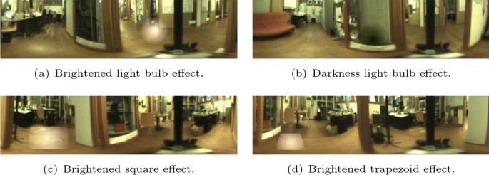

Individual local effects for data augmentation based on illumination

Global illumination::

Global illumination variations can occur in some cases. To model such illumination changes, we need to alter pixels across the whole image, rather than in a small region. A constant value $c$ is added to all the pixels to model a global brightness effect on the image or it is subtracted to simulate a global darkness. The value of $c$ varies from 35 to 75 in this work. Figure 4b and c shows the effect.

Sharpness/Blurring::

Finding sharper borders among diverse objects will contribute to provide a better separation among them and between foreground and background. In contrast, blurring effects are caused by low illumination and movements of the camera, which are common in mobile robotics. Both effects are incorporated in the data augmentation. They can be observed in Fig. 4d and e. Both can be achieved by a convolution operation using the following masks.

Fig. 4

Global effects for data augmentation

Sharpness effect	Blurring effect
$m_{sh}=\begin{bmatrix}{0}&{}{-1}&{}{0}\\ {-1}&{}{5}&{}{-1}\\ {0}&{}{-1}&{}{0}\end{bmatrix}$	$m_{bl}=\frac{1}{25}\begin{bmatrix}{1}&{}{1}&{}{1}&{}{1}&{}{1}\\ {1}&{}{1}&{}{1}&{}{1}&{}{1}\\ {1}&{}{1}&{}{1}&{}{1}&{}{1}\\ {1}&{}{1}&{}{1}&{}{1}&{}{1}\\ {1}&{}{1}&{}{1}&{}{1}&{}{1}\end{bmatrix}$

Contrast variation::

The contrast of the image plays an important role in highlighting different objects in the scene. Low contrast images usually look softer and with less shadows and reflections. The effect is proposed for this data augmentation to improve the robustness of the framework. The contrast is modified following the next equation:

$$\begin{aligned}I_s=64+c*(I-64)\end{aligned}$$

where $I_s$ is the resulting image, $I$ the original image and $c$ is the contrast factor. For $c>1$ the contrast increases and $c<1$ decreases the contrast. Additionally, an equalization of the image is also added to the data augmentation set. It evenly distributes the histogram values, which permits obtaining a new contrast augmentation effect. Figure 4f shows this effect.

Saturation changes::

The colour saturation of the image deals with the intensity of the colour. The less saturation, the less colourful the image is, even it can resemble a grey-scale image if the saturation is very low. In contrast, more vivid colours are obtained when the colour saturation is high. It can simulate situations when illumination changes significantly. The colour saturation can be edited by converting the RGB image to HSV, after that, it is possible to directly change the saturation channel by multiplying it by a constant factor c. If the saturation attribute is multiplied by $c>1$ the colours become more saturated and by $c<1$ the colour saturation decreases. The effect can be seen in Fig. 4g.

Rotation::

The original image covers 360° around the robot. For that reason the image can be rotated without losing any piece of information. This effect will simulate the situation in which the robot is in the same position but the orientation is different. Moreover, having a training dataset containing this type of effect is expected to provide the Neural Network with rotation invariance. Figure 4h shows a rotation effect of 115°. Random rotations between 10 and 350° are applied to the training images.

Combined changes::

Additionally some effects are combined to obtain a larger data augmentation, but not all the effects are combined together. Global illumination and a single local effect are combined in all the possible variations, e.g. global darkness is combined with a brightening circle shape effect, global brightness is combined with a brightening trapezoidal effect, etc. Additionally, the local effects are also combined. The circle shape effect is combined with the square effect, the trapezoidal effect or another circle shape effect, the combinations can be brightened+brightened, brightened+darkness and darkness+darkness; the circle shape effect is also combined with other two circle shape effects, obtaining an image with three light bulb effects. Finally, the rotation effect is individually combined with all the effects and the combinations described above.

4.3 Training and testing the Siamese Neural Network

As presented in Sect. 4.1, different CNNs architectures can be used as the base of Siamese Neural Networks. Initially, we start from pretrained networks with known weights and biases. Then, we retrain the network to fit it to our application. This transfer learning technique is well-known and has previously been used in mobile robotics (Cabrera et al. 2021).

Ssection 4.3.1 will address an initial task which consists in training and evaluating the capability of a Siamese Neural Network to identify whether two images were captured from the same or different rooms. Finally, in Sect. 4.3.2 we will detail the characteristics of the training and test to address the absolute localization problem with siamese architectures. Emphasis will be placed on the labelling required to perform the desired task.

4.3.1 Room Discrimination

The main goal of this task is to evaluate whether a Siamese Neural Network is capable of determining if two images belong to the same or different room. It is an important capability to perform localization tasks.

The training phase is performed by feeding the network with pairs of images. These pairs are labelled with 0 if they have been captured from the same room and 1 if not. The ratio same/different room pairs is varied in the training phase to study its influence.

During the test phase, pairs of images are fed into the network. At the output, the network labels them with a number between 0 and 1; if the result is under 0.5 we interpret that the images have been captured from the same room. On the contrary, the images belong to different rooms. The images used to test the network are different from the training images, they are captured in the same building but in different times, in a variety of lighting conditions. Also the trajectory followed by the robot to capture the test images is similar to the one used to capture the training images, but the images are captured from different robot poses (Fig. 5).

Fig. 5

Example of different trajectories of the robot

4.3.2 Global localization

The global localization problem considers the estimation of the robot pose within the whole floor of the building. For this purpose, a Siamese Neural Network is trained. The training is carried out with image pairs labelled with the following equation:

$$\begin{aligned} Label(I_i, I_j)= \left\{ \begin{array}{lcc} \frac{\Vert \vec {p}_i-\vec {p}_j\Vert _2}{K_b} &{} \textrm{if} ~I_{i}~ \textrm{and} ~I_{j}~ \mathrm {belong~ to ~the~ same ~room} \\ 1 &{} \textrm{otherwise} \end{array} \right. \end{aligned}$$

(2)

where $I_i$ and $I_j$ are two images and $\vec {p}_i$ and $\vec {p}_j$ are their corresponding positions (coordinates of the capture points). This constitutes a normalized Euclidean distance between the capture points. $K_b$ corresponds to the maximum distance between two images in the building. Table 5 shows different examples according to Fig. 5.

Table 5 Example pairs and its label value for the absolute localization task

Once the network has been trained, the test is performed by using the map which is composed by the set of image descriptors and their positions $\{(\vec {f}_1,\vec {p}_1),(\vec {f}_2,\vec {p}_2),\ldots ,(\vec {f}_N,\vec {p}_N)\}$. Each descriptor has been calculated by the trained Siamese Neural Network. The absolute localization is performed as a pairwise comparison between image descriptors. Given a test image $I_t$, the Siamese Neural Network outputs its corresponding descriptor $\vec {f}_t$. Finally, the position of the robot is estimated by selecting the pose associated to the descriptor in the map that minimizes the distance $\Vert \vec {f}_t-\vec {f}_i\Vert _2$, with $i = 1,\ldots , N$.

5 Experiments

The set of experiments is designed to test the performance of the Siamese Neural Network as global descriptor generator to tackle the room discrimination and global localization task as explained in Sects. 4.3.1 and 4.3.2.

5.1 Room Discrimination

In this subsection we assess the ability of the network to predict whether two images are taken from the same room. The effectiveness of the Siamese Neural Network is calculated by comparing pairs of images and checking their label. The results are expressed in percentage of accuracy. Several experiments have been conducted while varying different parameters: the feature extraction architecture, the feature aggregation layers and the percentage of similar/dissimilar images. As common parameters, we train the network using 8486 pairs of images per epoch from the training dataset 1 and we use the Stochastic Gradient Descent (SGD) optimiser, with a learning rate of 0.001 and momentum of 0.9. Moreover, we test the network with 7000 pairs of images extracted from the test dataset 4.

5.1.1 Influence of the architecture on the feature extraction process

In this subsection we compare different models in the feature extraction stage of a Siamese Neural Network. The different models used can be observed in Table 1. The training has been performed using a batch size of 256 and 5 epochs. During training, the dataloader presents a 50% of images from the same room and a 50% of images from the different rooms. During these experiments, the feature aggregation is performed with 3 fully connected layers composed by 500–500-5 neurons in each.

Results are presented in Table 6 in terms of global accuracy. Additionally, the test accuracy for the same and different room predictions is also presented. The table shows that the best networks are VGG13 and VGG16. They obtain the best accuracy for predicting pairs of images in the same room (99.44% and 99.47% respectively). In addition, VGG13 and VGG16 present the best accuracy predicting if two images are taken from different rooms (79.86% and 78.91%). Moreover, the ‘Simple 1’ and ‘Simple 2’ networks obtain considerably good results using only three convolutional layers. Finally, in general terms, it can be observed that all the architectures perform better in predicting whether two images belong to the same room. For this reason, we consider below the possibility of varying the percentage of images of each category in the training phase.

Table 6 Accuracy using different feature extraction neural networks. (Color table online)

5.1.2 Influence of the training parameters

In the light of the previous results, next, different training parameters are evaluated. As we explain in the previous subsection, the ratio of training pairs of images in each category is expected to have a substantial influence upon the results. In consequence, we propose to change the percentage of pairs of images at the training phase. The percentage of images taken from the same and different rooms varies from 5% to 40% and from 95% to 60% respectively. For brevity, we only show the results obtained with VGG13, VGG16 and AlexNet networks. The rest of the training parameters is tuned as before, using 256 as batch size and a feature aggregation phase with three fully connected layers composed by 500, 500 and 5 neurons. The results are presented in Tables 7, 8 and 9. They show a correlation between the percentage of images of same/different room and its respective accuracy, i. e., when the percentage of pairs of images in the same room increases, its associated accuracy also does and a similar phenomenon occurs with the different room category.

Table 7 Accuracy of VGG13. (Color table online)

Table 8 Accuracy of VGG16. (Color table online)

Table 9 Accuracy of AlexNet. (Color table online)

Until this moment, all the experiments have been performed using 256 as batch size, but other values have been tested in order to check the best configuration. Tables 10 and 11 show the accuracy using different batch sizes. They show that the global accuracy increases when the batch size is lower.

Table 10 Accuracy using VGG16 and different batch sizes. (Color table online)

Table 11 Accuracy using AlexNet and different batch sizes. (Color table online)

These tables show that relatively good performances can be achieved with some configurations. Notwithstanding that, we observe that in general terms, the same-room accuracy tends to decrease when the different-room accuracy increases and vice versa. This will be analyzed deeply in future works, but it may be due to the use of the Contrastive Loss function (Sun et al. 2020a).

5.1.3 Influence of the architecture of the feature aggregation layers

As explained in Sect. 4.1, the feature extraction layers output a matrix that is flattened and compressed in the feature aggregation phase. Different combinations of fully connected layers are also evaluated. All these experiments have been performed training the network with a 10 of pairs of images taken from the same room and a 90 of pairs of images from different rooms.

Tables 12 and 13 show the results using 3 different combinations of fully connected layers. Each variation is described in Table 3. Similar results are obtained with the 3 different variations. The best result is obtained with 3 fully connected layers with 1000-1000-10 neurons each. Finally, if we analyse jointly all the results of the room discrimination experiment, the best result is obtained using VGG16 as the feature extraction network, 3 fully connected layers (1000-1000-10), 7 epoch and a batch size of 16; with this configuration 96.16% global accuracy is obtained: 98.90% same room accuracy and 93.41% different room accuracy.

Table 12 Accuracy using VGG16 and different feature aggregation layers. (Color table online)

Table 13 Accuracy using AlexNet and feature aggregation layers. (Color table online)

5.2 Global localization

The global localization is performed as explained in Sect. 4.3.2. The VGG16 network is employed in this task since it led to the best results in the room discrimination task. Different experiments have been performed in order to choose the best configuration. We will mainly analyze the ratio of same/different room pairs, which is the parameter that has shown the greatest influence on the results. Moreover, in this subsection we will assess the influence of the data augmentation on the results. Each pair of images is labelled according Eq. 2.

First, concerning the experiment to evaluate the influence of the ratio same/different room pairs, we train the network using 8486 pairs of images per epoch from the training dataset 1. Second, with respect to the experiment to assess the effect of the data augmentation, 977,856 pairs of images per epoch from the training dataset 2 are used. These two experiments are described in Sect. 5.2.1. In both cases, the fully connected layers are configured with 500-500-5 neurons. Moreover, Sect. 5.2.2 evaluates the influence of the feature aggregation layers. In this case, the training dataset 1 is used. As common parameters, we use 16 as batch size, the Stochastic Gradient Descent (SGD) optimizer, with a learning rate of 0.001 and a momentum of 0.9 and 30 epochs.

5.2.1 Influence of the training parameters

Ratio of same/different room pairs::

Table 14 shows the results using VGG16 in the feature extraction part and three fully connected layers with 500-500-5 neurons in the feature aggregation part. The training of the model has been performed with different percentages of pairs of images belonging to the same and different rooms. The results show that the lowest localization error is obtained when the training is performed using 40% of images from the same room and 60% of images from different rooms. In general, The CNN shows excellent overall performance, especially when tested under the same lighting conditions as the training images (cloudy). However, the performance decreases in sunny conditions which are the most challenging test conditions. Studying the results, as a general rule, training with a large percentage of image pairs from the same room deteriorates the localization error.

Data Augmentation::

Next, we evaluate the influence of the data augmentation on the localization task. Table 15 presents the results using the training dataset 2 (augmented) and test datasets 1, 2 and 3. For this purpose, we will start from the best configurations obtained so far and show the results according to the percentage of training image pairs. When the training is performed with the augmented dataset, remarkable results in terms of average error are obtained, especially in cloudy and night conditions. In this sense, the Mean Average Error decreases by 10 cm in cloudy conditions and by 20 cm in night conditions comparing to Table 14 (no data augmentation). However, training with this dataset shows a decrease in the performance of the network in sunny circumstances. Therefore, the data augmentation proves to be beneficial, unless the test images experience substantial changes.

Table 14 Localization error in terms of mean absolute error (MAE), mean square error (MSE) and average recall (%) at top 1% (Recall@1%) with VGG16. (Color table online)

Table 15 Localization error in terms of mean absolute error (MAE), mean square error (MSE) and average recall (%) at top 1% (Recall@1%) with VGG16 and data augmentation. (Color table online)

5.2.2 Influence of the architecture of the feature aggregation layers

To conclude the experimental section, Table 16 shows the results after evaluating different fully connected layers. Using 4096-4096-1000 neurons in these three layers demonstrated a consistent localization error for cloudy and night conditions. However, its performance degraded in sunny conditions. When the size of the fully connected layers is 1000-1000-10 the best result in cloudy conditions is achieved, but also the worst result for sunny scenarios. In contrast, the configuration 500-500-5 neurons consistently maintained low errors across all conditions, showing its adaptability to diverse lighting environments and generalization capabilities. The Siamese Neural Network is able to perform the localization with an average error of 0.5821 m when using as feature aggregation method three different fully connected layers with 500, 500 and 5 neurons.

Table 16 Localization error in terms of mean absolute error (MAE), mean square error (MSE) and average recall (%) at top 1% (Recall@1%) with VGG16 and different configurations of the fully connected layers when training 30 epochs and 50% of images from the same room and 50% of images from different rooms. (Color table online)

5.2.3 General comparison with other methods

Finally, the Siamese Neural Networks are compared with other previous global-appearance techniques which include the use of a single AlexNet structure and two classic analytic descriptors: HOG and gist, as described in the work by Cebollada et al. (2022). Table 17 compares all the methods in a global localization task using, in all cases, the COLD-Freiburg Dataset. This table shows that the siamese structures with the VGG architecture and the data augmentation proposed in the present work provide the best results in terms of localization error for cloudy and night conditions. Also, the approach proposed by Rostkowska and Skrzypczyński (2023) achieves good results in the case of sunny conditions. Apart from using a different architecture, the main difference between their approach and the one presented here is that they use a cross-entropy loss (single input) during training, while in the present paper we employ the contrastive loss (double input). Furthermore, in the present paper, the model is fed with an omnidirectional image transformed to a panoramic view, whereas in Rostkowska and Skrzypczyński (2023) directly use the omnidirectional image without conversion. In addition, they embed the image with an EfficientNet model (Tan and Le 2019) architecture which is followed by the Facebook AI Similarity Search (FAISS) KD-Tree, while in the approach proposed in the present paper the pairwise euclidean distance between descriptors is computed and employed to retrieve the closest descriptor in the database.

Table 17 Comparison with other methods. (Color table online)

6 Conclusions

In this paper, a global localization method using Siamese Neural Networks has been proposed and evaluated. Localization, along with mapping, is one of the main tasks to be addressed by an autonomous mobile robot. First, an initial task of discriminating same and different rooms has been proposed in order to assess the ability of Siamese Neural Networs and know the influence of the most relevant parameters. After that, the global localization problem is addressed.

In the experiments, several well known architectures have been tested to conform the Siamese Neural Network, some of which are AlexNet, VGG11, VGG13, VGG16, VGG19, VGG11bn, VGG13bn, VGG16bn and VGG19bn. The best performance in the initial task has been achieved by VGG13 and VGG16. In general terms, the VGG architectures have provided the best results.

Apart from these feature extraction architectures, a group of Fully Connected layers have been added to carry out the conversion of the activation maps resulting from the convolutional layers to a description vector. In the present work, different sizes of the Fully Connected layers have been studied, as well as the size of the final descriptor. For the initial task, the performance of the network is slightly higher when the Fully Connected layers sizes are 1000-1000-10. In contrast, in the global localization, the localization error decreases drastically in those networks that have a set of Fully Connected layers of size 500-500-5 neurons.

The training parameter that contributes most to the performance of the network is the percentage of image pairs belonging to the same and different rooms. In this sense, there is a correlation between the percentage of images of same/different room and its respective accuracy, i.e., when the percentage of pairs of images in the same room increases, its associated accuracy also does and a similar effect occurs with the different room category. Furthermore, when the same room accuracy increases, the different room accuracy decreases, and vice versa. This situation may be caused by the Contrastive Loss function which has an associated lack of flexibility in the optimization. Other loss functions used in other applications could improve localization results, such as Circle Loss (Sun et al. 2020b) and will be considered in future studies.

In addition, a data augmentation technique has been proposed in order to improve the performance of the network. The proposed effects try to simulate real operating conditions. In addition, a set of effects specially designed to increase the robustness against changes of the lighting conditions in the scene have been generated. As for the results obtained, the performance of the network is especially benefited when working in cloudy and night lighting conditions. In the case of the cloudy lighting condition, when the training is performed with data augmentation, the average localization error is reduced around 12 cm. As for the night illumination condition, the average error is reduced around 20 cm. On the contrary, in sunny illumination condition the average localization error increases 34 cm when data augmentation is used. Thus, the siamese architecture is very efficient at solving the localization problem in real operating conditions, if the changes in the lighting conditions are not considerable, i.e., when working in cloudy and night scenarios. However, it is less effective at describing images in the presence of significant changes in lighting conditions, such as in the sunny scenarios. Other methods (such as HOG or gist) describe the image globally and give equal importance to all its regions, thus providing better resilience to large illumination changes. The reduced performance on sunny conditions when using siamese architectures can be explained by the lack of flexibility associated to the fact of having two networks with identical weights. In addition, the training process may have introduced an imbalance that causes the network to be more capable of detecting similarities than dissimilarities or vice versa. Additionally, the training dataset 1 (without data augmentation) comprises images from all illumination conditions, whereas the training dataset 2 (with data augmentation) is limited to cloudy images and attempts to replicate other illumination conditions by applying global and local effects. In this context, the proposed effects for data augmentation are beneficial in cloudy and night conditions, thus enhancing the performance of the model in these scenarios. However, the illumination effects that simulate different sunny conditions have been proven to be less effective than using real images captured at this particular illumination condition.

As future works, the proposed localization techniques will be extended to outdoor environments, which are more challenging because of their unstructured and changing conditions. In addition, other types of sensors will be considered to carry out the localization robustly, such as LiDAR.

References

Arandjelovic R, Gronat P, Torii A, Pajdla T, Sivic J (2016) NetVLAD: CNN architecture for weakly supervised place recognition. In: Proceedings of the IEEE conference on computer vision and pattern recognition, pp 5297–5307
Ballesta M, Payá L, Cebollada S, Reinoso O, Murcia F (2021) A CNN regression approach to mobile robot localization using omnidirectional images. Appl Sci 11(16):7521
Bayraktar E, Yigit CB, Boyraz P (2019) A hybrid image dataset toward bridging the gap between real and simulation environments for robotics: annotated desktop objects real and synthetic images dataset: ADORESet. Mach Vis Appl 30(1):23–40
Bayraktar E, Yigit CB, Boyraz P (2020) Object manipulation with a variable-stiffness robotic mechanism using deep neural networks for visual semantics and load estimation. Neural Comput Appl 32(13):9029–9045
Bromley J, Guyon I, LeCun Y, Säckinger E, Shah R (1993) Signature verification using a “Siamese” time delay neural network. In: Advances in neural information processing systems (NIPS 1993), vol 6. Morgan Kaufmann, San Mateo
Cabrera JJ, Cebollada S, Payá L, Flores M, Reinoso Ó (2021) A robust CNN training approach to address hierarchical localization with omnidirectional images. In: ICINCO, pp 302–310
Cao L, Ling J, Xiao X (2020) Study on the influence of image noise on monocular feature-based visual SLAM based on FFDNet. Sensors 20(17):4922
Cattaneo D, Vaghi M, Ballardini AL, Fontana S, Sorrenti DG, Burgard W (2019) CMRNET: camera to lidar-map registration. In 2019 IEEE intelligent transportation systems conference (ITSC). IEEE, pp 1283–1289
Cebollada S, Payá L, Román V, Reinoso O (2019) Hierarchical localization in topological models under varying illumination using holistic visual descriptors. IEEE Access 7:49580–49595
Cebollada S, Payá L, Flores M, Peidró A, Reinoso O (2020) A state-of-the-art review on mobile robotics tasks using artificial intelligence and visual data. Expert Syst Appl 167:114195
Cebollada S, Payá L, Jiang X, Reinoso O (2022) Development and use of a convolutional neural network for hierarchical appearance-based localization. Artif Intell Rev 55(4):2847–2874
Chen X, Läbe T, Milioto A, Röhling T, Behley J, Stachniss C (2022) OverlapNet: a siamese network for computing lidar scan similarity with applications to loop closing and localization. Auton Robot 46(1):61–81
Chollet F et al (2018) Deep learning with Python, vol 361. Manning, New York
Rublee E, Rabaud V, Konolige K, Bradski G(2011) ORB: an efficient alternative to SIFT or SURF. In: IEEE International conference on computer vision, ICCV 2011, pp 2564–2571
Feng Q, Shum HP, Morishima S (2020) Resolving hand-object occlusion for mixed reality with joint deep learning and model optimization. Comput Anim Virtual Worlds 31(4–5):e1956
Hadsell R, Chopra S, LeCun Y (2006) Dimensionality reduction by learning an invariant mapping. In: 2006 IEEE computer society conference on computer vision and pattern recognition (CVPR’06), vol 2. IEEE, pp 1735–1742
He K, Zhang X, Ren S, Sun J (2016) Deep residual learning for image recognition. In: Proceedings of the IEEE conference on computer vision and pattern recognition, pp 770–778
Holliday A, Dudek G (2018) Scale-robust localization using general object landmarks. In: 2018 IEEE/RSJ international conference on intelligent robots and systems (IROS). IEEE, pp 1688–1694
Hu S, Shum HP, Liang X, Li FW, Aslam N (2021) Facial reshaping operator for controllable face beautification. Expert Syst Appl 167:114067
Hu Y, Shum HP, Ho ES (2020) Multi-task deep learning with optical flow features for self-driving cars. IET Intell Transp Syst 14(13):1845–1854
Jeon M, Park D, Lee J, Jeon H, Ko M, Kim S, Choi Y, Tan AC, Kang J (2019) ReSimNet: drug response similarity prediction using Siamese neural networks. Bioinformatics 35(24):5249–5256
Johnson J, Douze M, Jégou H (2019) Billion-scale similarity search with GPUs. IEEE Trans Big Data 7(3):535–547
Junior JM, Tommaselli A, Moraes M (2016) Calibration of a catadioptric omnidirectional vision system with conic mirror. ISPRS J Photogramm Remote Sens 113:97–105
Khaliq A, Ehsan S, Chen Z, Milford M, McDonald-Maier K (2019) A holistic visual place recognition approach using lightweight CNNs for significant viewpoint and appearance changes. IEEE Trans Robot 36(2):561–569
Korrapati H, Mezouar Y (2017) Multi-resolution map building and loop closure with omnidirectional images. Auton Robot 41(4):967–987
Krizhevsky A, Sutskever I, Hinton GE (2012) ImageNet classification with deep convolutional neural networks. Adv Neural Inf Process Syst 25:1097–1105
Leyva-Vallina M, Strisciuglio N, Lopez-Antequera M, Tylecek R, Blaich M, Petkov N (2019) Tb-places: A data set for visual place recognition in garden environments. IEEE Access 7:52277–52287
Leyva-Vallina M, Strisciuglio N, Petkov N (2019) Place recognition in gardens by learning visual representations: data set and benchmark analysis. In: International conference on computer analysis of images and patterns. Springer, pp 324–335
Leyva-Vallina M, Strisciuglio N, Petkov N (2021) Generalized contrastive optimization of siamese networks for place recognition. arXiv preprint. arXiv:2103.06638
Li Y, Zhang X (2019) SiamVGG: visual tracking using deeper siamese networks. arXiv preprint. arXiv:1902.02804
Lin J, Peng J, Hu Z, Xie X, Peng R et al (2020) ORB-SLAM, IMU and wheel odometry fusion for indoor mobile robot localization and navigation. Acad J Comput Inf Sci 3(1):131–141
Liu W, Mo Y, Jiao J (2019) An efficient edge-feature constraint visual SLAM. In: Proceedings of the international conference on artificial intelligence, information processing and cloud computing, pp 1–7
Lu Y, Lu G (2019) Deep unsupervised learning for simultaneous visual odometry and depth estimation. In: 2019 IEEE international conference on image processing (ICIP). IEEE, pp 2571–2575
Ma L, Chen J et al (2019) Using RGB image as visual input for mapless robot navigation. arXiv preprint. arXiv:1903.09927
Moolan-Feroze O, Karachalios K, Nikolaidis DN, Calway A (2019) Improving drone localisation around wind turbines using monocular model-based tracking. In: 2019 International conference on robotics and automation (ICRA). IEEE, pp 7713–7719
Organisciak D, Sakkos D, Ho ES, Aslam N, Shum HP (2020) Unifying person and vehicle re-identification. IEEE Access 8:115673–115684
Parajuli N, Lu A, Stendahl JC, Zontak M, Boutagy N, Alkhalil I, Eberle M, Lin BA, O’Donnell M, Sinusas AJ et al (2017) Flow network based cardiac motion tracking leveraging learned feature matching. In: International conference on medical image computing and computer-assisted intervention. Springer, pp 279–286
Polvara R, Sharma S, Wan J, Manning A, Sutton R (2018) Obstacle avoidance approaches for autonomous navigation of unmanned surface vehicles. J Navig 71(1):241–256
Pronobis A, Caputo B (2009) COsy localization database. Int J Robot Res (IJRR) 28(5):588–594. https://doi.org/10.1177/0278364909103912
Mur-Artal R, Montiel JMM, Tardós JD (2015) ORB-SLAM: a versatile and accurate monocular SLAM system. IEEE Trans Robot. https://doi.org/10.1109/TRO.2015.2463671
Rituerto A, Puig L, Guerrero JJ (2010) Visual SLAM with an omnidirectional camera. In: 2010 20th International conference on pattern recognition. IEEE, pp 348–351
Rostkowska M, Skrzypczyński P (2023) Optimizing appearance-based localization with catadioptric cameras: small-footprint models for real-time inference on edge devices. Sensors 23(14):6485
Ruan X, Ren D, Zhu X, Huang J (2019) Mobile robot navigation based on deep reinforcement learning. In: 2019 Chinese control and decision conference (CCDC). IEEE, pp 6174–6178
Sakkos D, Shum HP, Ho ES (2019) Illumination-based data augmentation for robust background subtraction. In: 2019 13th International conference on software, knowledge, information management and applications (SKIMA). IEEE, pp 1–8
Sandouk U, Chen K (2017) Learning contextualized music semantics from tags via a siamese neural network. ACM Trans Intell Syst Technol 8(2):24
Schaupp L, Bürki M, Dubé R, Siegwart R, Cadena C (2019). OREOS: oriented recognition of 3d point clouds in outdoor scenarios. In 2019 IEEE/RSJ international conference on intelligent robots and systems (IROS). IEEE, pp 3255–3261
Simonyan K, Zisserman A (2014) Very deep convolutional networks for large-scale image recognition. arXiv preprint. arXiv:1409.1556
Sinha H, Patrikar J, Dhekane EG, Pandey G, Kothari M (2018) Convolutional neural network based sensors for mobile robot relocalization. In: 2018 23rd International conference on methods & models in automation & robotics (MMAR). IEEE, pp 774–779
Suljagic H, Bayraktar E, Celebi N (2022) Similarity based person re-identification for multi-object tracking using deep siamese network. Neural Comput Appl 34(20):18171–18182
Sun Y, Cheng C, Zhang Y, Zhang C, Zheng L, Wang Z, Wei Y (2020) Circle loss: a unified perspective of pair similarity optimization. In: Proceedings of the IEEE/CVF conference on computer vision and pattern recognition, pp 6398–6407
Szegedy C, Liu W, Jia Y, Sermanet P, Reed S, Anguelov S, Erhan D, Vanhoucke V, Rabinovich A (2015) Going deeper with convolutions. In: Proceedings of the IEEE conference on computer vision and pattern recognition, pp 1–9
Tan M, Le Q (2019) EfficientNet: rethinking model scaling for convolutional neural networks. In International conference on machine learning. PMLR, pp 6105–6114
Thiolliere R, Dunbar E, Synnaeve G, Versteegh M, Dupoux E (2015) A hybrid dynamic time warping-deep neural network architecture for unsupervised acoustic modeling. In: 16th annual conference of the international speech communication association
Utkin LV, Zaborovsky VS, Popov SG (2017) Siamese neural network for intelligent information security control in multi-robot systems. Autom Control Comput Sci 51(8):881–887
Wang Y, Bao T, Ding C, Zhu M (2017) Face recognition in real-world surveillance videos with deep learning method. In: 2017 2nd international conference on image, vision and computing (ICIVC). IEEE, pp 239–243
Weinzaepfel P, Csurka G, Cabon Y, Humenberger M (2019) Visual localization by learning objects-of-interest dense match regression. In: Proceedings of the IEEE/CVF conference on computer vision and pattern recognition, pp 5634–5643
Xu S, Chou W, Dong H (2019) A robust indoor localization system integrating visual localization aided by CNN-based image retrieval with Monte Carlo localization. Sensors 19(2):249
Yin H, Tang L, Ding X, Wang Y, Xiong R (2018) LocNet: global localization in 3d point clouds for mobile vehicles. In: 2018 IEEE intelligent vehicles symposium (IV). IEEE, pp 728–733
Zaki HF, Shafait F, Mian A (2019) Viewpoint invariant semantic object and scene categorization with RGB-D sensors. Auton Robot 43(4):1005–1022
Zeng A, Song S, Yu KT, Donlon E, Hogan FR, Bauza M, Ma D, Taylor O, Liu M, Romo E et al (2018) Robotic pick-and-place of novel objects in clutter with multi-affordance grasping and cross-domain image matching. In: 2018 IEEE international conference on robotics and automation (ICRA). IEEE, pp 3750–3757
Zhang Z, Peng H (2019) Deeper and wider Siamese networks for real-time visual tracking. In: Proceedings of the IEEE/CVF conference on computer vision and pattern recognition, pp 4591–4600
Zhao Q, Zhang B, Lyu S, Zhang H, Sun D, Li G, Feng W (2018) A CNN-SIFT hybrid pedestrian navigation method based on first-person vision. Remot Sens 10(8):1229
Zheng W, Yang L, Genco RJ, Wactawski-Wende J, Buck M, Sun Y (2019) Sense: Siamese neural network for sequence embedding and alignment-free comparison. Bioinformatics 35(11):1820–1828
Zhong F, Wang S, Zhang Z, Wang Y (2018) Detect-SLAM: Making object detection and SLAM mutually beneficial. In: 2018 IEEE winter conference on applications of computer vision (WACV). IEEE, pp 1001–1010
Acknowledgements
The Ministry of Science, Innovation and Universities (Spain) has supported this work through “Ayudas para la Formación de Profesorado Universitario” (FPU21/04969). This work is also part of the project TED2021-130901B-I00, funded by MCIN/AEI/10.13039/501100011033 and by the European Union “NextGenerationEU”/PRTR, and of the project PID2020-116418RB-I00 funded by MCIN/AEI/10.13039/501100011033.
Funding
Open Access funding provided thanks to the CRUE-CSIC agreement with Springer Nature.
Author information
Authors and Affiliations
Contributions
Conceptualization, J.J.C., V.R. and L.P.; methodology, J.J.C., V.R. and A.G.; software, J.J.C. and V.R.; validation, J.J.C. and V.R. ; formal analysis, A.G. and L.P.; writing (original draft preparation), V.R. and J.J.C.; writing (review and editing), A.G., L.P. and O.R.; supervision, A.G., L.P. and O.R.; Project administration L.P. and O.R.
Corresponding author
Ethics declarations
Competing interests
The authors declare no competing interests.
Additional information
Publisher's Note
Springer Nature remains neutral with regard to jurisdictional claims in published maps and institutional affiliations.
Rights and permissions
Open Access This article is licensed under a Creative Commons Attribution 4.0 International License, which permits use, sharing, adaptation, distribution and reproduction in any medium or format, as long as you give appropriate credit to the original author(s) and the source, provide a link to the Creative Commons licence, and indicate if changes were made. The images or other third party material in this article are included in the article's Creative Commons licence, unless indicated otherwise in a credit line to the material. If material is not included in the article's Creative Commons licence and your intended use is not permitted by statutory regulation or exceeds the permitted use, you will need to obtain permission directly from the copyright holder. To view a copy of this licence, visit http://creativecommons.org/licenses/by/4.0/.
About this article
Cite this article
Cabrera, J.J., Román, V., Gil, A. et al. An experimental evaluation of Siamese Neural Networks for robot localization using omnidirectional imaging in indoor environments. Artif Intell Rev 57, 198 (2024). https://doi.org/10.1007/s10462-024-10840-0
Published:
DOI: https://doi.org/10.1007/s10462-024-10840-0