Bifurcations in Volume-Preserving Systems

Abstract

We give a survey on local and semi-local bifurcations of divergence-free vector fields. These differ for low dimensions from ‘generic’ bifurcations of structure-less ‘dissipative’ vector fields, up to a dimension-threshold that grows with the co-dimension of the bifurcation.

1 Introduction

Local bifurcations are bifurcations of equilibria of vector fields and bifurcations of fixed points for mappings. The latter can always be interpreted as Poincaré mappings, see [23], with the fixed points giving rise to periodic orbits, which in principle can be of non-local influence. However, the term semi-local bifurcation is usually reserved for bifurcations of invariant tori in dynamical systems—whether given by the flow of a vector field or by iterating an invertible mapping. All these invariant sets can be attractors for dynamical systems that are dissipative; in particular for generic dynamical systems that preserve no structure whatsoever. But also e.g. reversible systems do admit attractors (together with a repelling counterpart obtained by applying the reversing symmetry to the attractor).

Bifurcations of strange attractors count as global bifurcations as do bifurcations of other invariant sets—think of stable and unstable manifolds and invariant sets like horseshoes. These other bifurcations can also take place in structure-preserving dynamical systems, like Hamiltonian systems or volume-preserving systems. Still the best understood examples of such global bifurcations are subordinate to local or semi-local bifurcations. Similarly, bifurcations of invariant tori are best treatable where they originate from local bifurcations and concern invariant tori with a conditionally periodic flow. For suitable co-ordinates $x = (x_{1}, \ldots , x_{n}) \in \mathbb {T}^{n}$, $\mathbb {T}= \mathbb {R}/ \mathbb {Z}$ the equations of motion read

$$\dot{x} \;\; = \;\; \omega (\mu ) $$

and where the components $\omega _{1}, \ldots , \omega _{n}$ of the frequency vector $\omega \in \mathbb {R}^{n}$ are rationally independent the flow is in fact quasi-periodic.

As starting point we therefore take a family of conditionally periodic $n$-tori on an $({n+m})$-dimensional manifold with an oriented volume, where the $n$-tori are invariant under the flow of a volume-preserving vector field. While any manifold can carry a Borel measure, such a measure is defined in terms of a volume form if and only if the manifold is orientable. In that case we speak of an oriented volume. In local co-ordinates $(x, z)$ around the tori the equations of motion can be given the form

$$\begin{aligned} \dot{x} & \;\; = \;\; \omega (\mu ) \; + \; \mathcal {O}(z) \end{aligned}$$

(1a)

$$\begin{aligned} \dot{z} & \;\; = \;\; \varOmega (x; \mu ) \, z \; + \; \mathcal {O}\bigl(z^{2}\bigr) \end{aligned}$$

(1b)

where $\mu \in \mathbb {R}^{s}$ denotes the parameter(s) the family depends upon. In the periodic case $n=1$ this form can be further simplified to an $x$-independent $\varOmega = \varOmega (\mu )$ by Floquet’s Theorem [23]. In the quasi-periodic case $n \geq 2$ it is not always possible to remove the $x$-dependence of $\varOmega$ in (1b) and we merely assume the tori to be reducible to Floquet form. The system $(1)$ with $\varOmega = \varOmega (\mu )$ describes a family of vector fields on $\mathbb {T}^{n} \times \mathbb {R}^{m}$ with invariant tori $\mathbb {T}^{n} \times \{ 0 \}$ for every $\mu \in \mathbb {R}^{s}$. These tori have Floquet exponents $\beta _{j}(\mu ) + \mathrm {i}\alpha _{j}(\mu )$, $\alpha _{j}, \beta _{j} \in \mathbb {R}$ satisfying $\alpha _{2j} = - \alpha _{2j-1}$ for $j = 1, \ldots , \ell$ where $\alpha _{2j-1} > 0$ and, since $\operatorname {trace}\varOmega = 0$,

$$ \sum_{j=1}^{m} \beta _{j}(\mu ) + \mathrm {i}\alpha _{j}(\mu ) \;\; \equiv \;\; 0 \enspace . $$

(2)

In general the higher order terms $\mathcal {O}(z)$ and $\mathcal {O}(z^{2})$ in (1a) and (1b) depend on $x$, but where it is possible to pass to $x$-independent higher order terms in (1b)—e.g. by truncating a suitable normal form—the equations in $(1)$ decouple and one can first study the (relative) equilibria of (1b) in their own right.

The ultimate question is how the dynamics close to the family of invariant $n$-tori behaves under small perturbations. Near $\mathbb {T}^{n} \times \{ 0 \}$ the variable $z \in \mathbb {R}^{m}$ is small, therefore the higher order terms $\mathcal {O}(z)$ and $\mathcal {O}(z^{2})$ may already be considered as a perturbation. The corresponding unperturbed flow

$$ \textstyle\begin{array}{ccc} \mathbb {R}\times \mathbb {T}^{n} \times \mathbb {R}^{m} & \longrightarrow & \mathbb {T}^{n} \times \mathbb {R}^{m} \\ (t, x, z) & \mapsto & (x + t \!\: \omega (\mu ), \mathrm {e}^{t \!\: \varOmega (\mu )} \, z) \end{array} $$

(3)

is the superposition of a conditionally periodic motion on $\mathbb {T}^{n}$ with fixed (internal) frequency $\omega (\mu )$ and a linear flow on $\mathbb {R}^{m}$. Note that (3) is equivariant with respect to the $\mathbb {T}^{n}$-action

$$ \textstyle\begin{array}{ccc} \mathbb {T}^{n} \times \mathbb {T}^{n} \times \mathbb {R}^{m} & \longrightarrow & \mathbb {T}^{n} \times \mathbb {R}^{m} \\ (\xi , x, z) & \mapsto & (x + \xi , z) \enspace . \end{array} $$

(4)

If $\varOmega$ as well as the higher order terms $\mathcal {O}(z)$ and $\mathcal {O}(z ^{2})$ in $(1)$ are $x$-independent, the vector field is called $\mathbb {T}^{n}$-symmetric. Such vector fields have invariant $n$-tori $\mathbb {T}^{n} \times \{ z_{0} \}$ whenever the right hand side of (1b) vanishes at $z_{0}$. Where these tori have non-zero Floquet exponents one can locally near $\mathbb {T}^{n} \times \{ z_{0} \}$ put the equations of motion into the form $(1)$, with $\varOmega = \varOmega (\mu )$ and higher order terms independent of $x$. What happens under small perturbations is the realm of kam Theory.

Indeed, resonant tori are expected to be destroyed by the perturbation, while (strongly!) non-resonant tori can be shown to persist if the perturbation is sufficiently small—which means very small as there are no further conditions on the perturbation except for preserving the structure at hand. In frequency space both resonant and non-resonant frequency vectors $\omega \in \mathbb {R}^{n}$ form dense subsets and it is here that the dependence $\mu \mapsto \omega ( \mu )$ on the parameter $\mu \in \mathbb {R}^{s}$ becomes important. If the frequency mapping $\omega : \mathbb {R}^{s} \longrightarrow \mathbb {R}^{n}$ is a submersion—which requires $s \geq n$—then the set of strongly non-resonant tori is of full measure, see below, and kam Theory allows to conclude persistence of most quasi-periodic tori. On the other hand, the perturbation generically—within the universe of admissible perturbations, preserving the structure at hand—opens up the dense resonances to an open (albeit of small masure) complement of the union of persistent tori. We colloquially say that the corresponding non-persistent tori disappear in a resonance gap.

A family of normally hyperbolic tori $\mathbb {T}^{n} \times \{ 0 \} \times \{ \mu \}$, $\beta _{j}(\mu ) \neq 0$ for all $j = 1, \ldots , m$ and all $\mu \in \mathbb {R}^{s}$ typically persists under small perturbations when restricted to the ‘Cantor set’ defined by the Diophantine conditions

$$ \bigl|2 \pi \bigl\langle k \bigm| \omega (\mu ) \bigr\rangle \; + \; \bigl\langle \ell \bigm| \alpha (\mu ) \bigr\rangle \bigr| \;\; \geq \;\; \frac{\gamma }{|k|^{\tau }} \qquad \mbox{for all $0 \neq k \in \mathbb {Z}^{n}$ and $\ell \in \mathbb {Z}^{m}$ with $|\ell | \leq 2$,} $$

(5)

where $\langle x \mid y \rangle = {\displaystyle \sum }x_{j} y_{j}$ is the standard inner product, $|k| = |k_{1}| + \cdots + |k_{n}|$, $\gamma > 0$ and $\tau > n-1$. This is the condition of strong non-resonance alluded to above; the set of all Diophantine frequency vectors has large relative measure as its complement is of measure $\gamma$ as $\gamma \to 0$, see [8, 15] and references therein.

The topological ‘size’ of this measure-theoretically large set is ‘small’ as the complement is open and dense. Locally in the frequency space $\mathbb {R}^{n+m}$ this set has a product structure: half lines times a Cantor set. Indeed, when $(\omega , \alpha )$ satisfies (5) then also $(\varsigma \omega , \varsigma \alpha )$ satisfies (5) for all $\varsigma \geq 1$. The intersection of the set of all Diophantine frequency vectors with a sphere of radius $R > 0$ is closed and totally disconnected; by the theorem of Cantor–Bendixson [25] it is the union of a countable and a perfect set, the latter necessarily being a Cantor set.

The Diophantine conditions (5) provide for an effective bound away from the resonances, see [8, 34, 40] and references therein. However, for a parameter dependent family $(1)$ we can no longer expect that all tori are normally hyperbolic—under parameter variation one or several $\beta _{j}(\mu )$ may pass through 0. Of course, the more $\beta _{j}(\mu )$ are simultaneously vanishing, the higher the co-dimension. While the Implicit Mapping Theorem still allows to achieve the form $(1)$ if the corresponding $\alpha _{j}(\mu _{0})$ are non-zero where $\beta _{j}(\mu _{0}) = 0$, the case of Floquet tori with vanishing Floquet exponent(s) $\beta _{j}(\mu _{0}) + \mathrm {i}\alpha _{j}(\mu _{0}) = 0$ only allows to achieve

$$\begin{aligned} \dot{x} & \;\; = \;\; \omega (\mu ) \; + \; \mathcal {O}(z) \end{aligned}$$

(6a)

$$\begin{aligned} \dot{z} & \;\; = \;\; \sigma (\mu ) \; + \; \varOmega (\mu ) \, z \; + \; \mathcal {O}\bigl(z^{2}\bigr) \end{aligned}$$

(6b)

with $\sigma (\mu ) \in \ker \varOmega (\mu _{0})^{\mathrm {T}}$, see [11, 34, 40] and references therein. This makes it preferable to denote invariant $n$-tori as $\mathbb {T}^{n} \times \{ z _{0} \} \times \{ \mu _{0} \} \subseteq \mathbb {T}^{n} \times \mathbb {R}^{m} \times \mathbb {R}^{s}$ where the zeroes $(z_{0}, \mu _{0})$ of the right hand side of (6b) typically form an $s$-parameter family. For $(1)$ this family boils down to $\mathbb {T}^{n} \times \{ 0 \} \times \mathbb {R}^{s}$.

The simplest bifurcation for dissipative vector fields is the quasi-periodic saddle-node bifurcation [4, 11, 40] with $m=1$ and (6b) becoming $\dot{z} = \mu - z^{2}$, i.e.$\sigma (\mu ) \equiv \mu$ and $\varOmega (\mu ) \equiv 0$. This example shows that it is in general not possible to achieve $\sigma (\mu ) \equiv 0$, while $\sigma (\mu _{0}) = 0$ can always be achieved. The other two quasi-periodic bifurcations of co-dimension 1 that structure-less dissipative vector fields may undergo are the quasi-periodic Hopf bifurcation [3, 4, 11] and the frequency-halving or quasi-periodic flip bifurcation [4, 9, 11]. For both bifurcations $\sigma (\mu ) \equiv 0$ can be achieved. While the former needs $m \geq 2$ normal dimensions, the latter can be put into the form $(6)$ only after the passage to a $2{:}1$ covering space.

Remarks 1

• Research of bifurcations in volume-preserving systems started with Broer et al. [5, 6, 13, 16]. This is an interesting class of dynamical systems, where the standard techniques of transversality, normal forms, stability and instability could be applied, combined with kam Theory. One of the results concerns the occurrence of infinitely many moduli of stability and another that of infinite (c.q. exponential) flatness.

• The Shilnikov bifurcation concerns the 2-dimensional stable manifold of a 3-dimensional saddle point with a complex conjugate pair of eigenvalues $\beta \pm \mathrm {i}\alpha$, $\alpha \neq 0$, $\beta < 0$ containing the 1-dimensional unstable manifold as a homoclinic orbit spiralling back to the saddle. This bifurcation was first studied by Shil’nikov and Gavrilov in [22, 37] for dissipative systems but it also occurs in volume-preserving systems, where the stable eigenvalue is given by $-2 \beta > 0$ as dictated by (2). The Shilnikov bifurcation occurs subordinately in the Hopf–Saddle Node bifurcation, both in the dissipative and volume-preserving context. In the present paper the latter case is termed the “volume-preserving Hopf bifurcation” as this is the counterpart of the (dissipative) Hopf bifurcation for volume-preserving systems. As can be inferred from Fig. 1 below this involves a spherical structure consisting of 2-dimensional invariant manifolds, enclosing a Cantor foliation of invariant 2-tori shrinking down to an elliptic periodic orbit. René Thom [private communication] here spoke of “smoke rings”.

  Fig. 1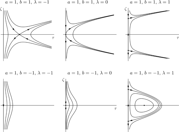

  

  Phase portraits of the planar reduced system as the bifurcation parameter $\lambda$ passes through 0 for the hyperbolic ($a=b=1$) and the elliptic ($a = 1$, $b = -1$) volume-preserving Hopf bifurcations

• The persistence of the quasi-periodic invariant tori inside the spherical structure as described above was first proven by Broer and Braaksma in [2, 7], using kam techniques.

• Another local study on volume-preserving vector fields is given by Gavrilov [21]. As in [5, 6, 13, 16] the classification is modulo topological equivalence. In dimension 2 the analysis essentially reduces to catastrophe theory on corresponding Hamiltonian functions. Again the focus is on the dimensions 3 or 4.

• Dullin and Meiss [19] study the dynamics of a family of volume-preserving diffeomorphisms on $\mathbb {R}^{3}$. This family unfolds a bifurcation of codimension 2, triggered by a fixed point with a triple Floquet multiplier 1. As in the above case of vector fields a spherical structure emerges, termed “vortex bubble” in [19]. In this spherical structure a Shilnikov–like situation occurs, where the inclusion of the 1-dimensional unstable manifold in the 2-dimensional stable manifold is replaced by sequences of generic tangencies. This setting involves both invariant circles and invariant 2-tori for the diffeomorphism. In particular, a string of pearls occurs that creates multiple copies of the original spherical structure for an iterate of the mapping.

• Lomelí and Ramírez-Ros [30] concentrate on the splitting of separatrices as the stable and unstable manifold forming the above spherical structure (for which they use the terms spheromak and Hill’s spherical vortices) cease to coincide due to a volume-preserving perturbation.

• Meiss et al. [33] also consider 3-dimensional diffeomorphisms, where chaotic orbits are studied near the spherical structure described above. In particular it is found that trapping times exhibit an algebraic decay.

Hofbauer and Sigmund [28] use volume-preserving systems for biological applications. They consider evolutionary models in terms of evolutionary game theory as this was initiated by the British mathematician and mathematical biologist John Maynard Smith [32], adapted to a setting with two populations. As suggested by Schuster, Sigmund et al. [27, 35, 36] this leads to an evolutionary dynamical system

$$\begin{aligned} \dot{x}_{i} = & x_{i} \bigl( (Ay)_{i} - \langle x \mid Ay \rangle \bigr) \enspace , \quad i = 0, 1, \ldots , n \\ \dot{y}_{j} = & y_{j} \bigl( (Bx)_{j} - \langle y \mid Bx \rangle \bigr) \enspace , \quad j = 0, 1, \ldots , m \end{aligned}$$

defined on $S_{n} \times S_{m}$. Here $S_{n} := \{ x \in \mathbb {R}^{n+1} \mid x_{i} \geq 1, \sum x_{i} = 1 \}$ is the unit simplex, related to a probability space.

An example is given by the battle of the sexes where the two populations are males and females and where the conflict is about the raising of offspring. The two strategies for males are philandering versus being faithful, while females have the choice between fast and coy, i.e. insisting on a long courtship. In the case where $n = m = 1$ the system is smoothly equivalent (in the dynamical sense) to a Hamiltonian system with Hamiltonian

$$H(x, y) \;\; = \;\; a \log y \; + \; b \log (1-y) \; + \; c \log x \; + \; d \log (1-x) \enspace . $$

This gives a kind of dynamics similar to the classical Lotka–Volterra predator prey systems, with all orbits periodic. What happens in the case of general $(n, m)$?

For general $(n, m)$ it turns out that the system, up to smooth dynamical equivalence, preserves a certain volume form that explodes at the boundary of $S_{n} \times S_{m}$. This property was discovered by Akin, see [20]. This means that the dynamics can be imagined as the motion of a particle in an incompressible fluid.

As an example the case where $n = m = 2$ is considered, where the theory of [6, 7] is used, including the reduced planar phase portraits, see Figs. 1 and 2 below. Also [9] is invoked to explain the occurrence of invariant 3-tori that form a recurrent set of positive measure. The existence of an intermediate chaotic regime is already suspected in [26].

Fig. 2

Phase portraits of the planar reduced system as the bifurcation parameter $\lambda$ passes through 0 for the hyperbolic ($c_{1} = 1$, $c_{2} = -1$) and elliptic ($c_{1} = c_{2} = 1$) cases of the volume-preserving double Hopf bifurcation

This paper is organized as follows. In the next three sections we focus on the normal dynamics defined by (6b) with $x$-independent higher order terms $\mathcal {O}(z^{2})$. This covers the case $n=0$ of equilibria, of which we describe the linear theory in Sect. 2 and the nonlinear theory in Sects. 3 and 4. The case $n=1$ of periodic orbits then is addressed in Sect. 5. In Sect. 6 we come back to quasi-periodic bifurcations in volume-preserving dynamical systems and Sect. 7 concludes the paper.

2 Linear Systems

In this section we treat linear systems $\dot{z} = \varOmega z$ on $\mathbb {R}^{m}$ that preserve the standard volume, i.e. satisfy $\operatorname {trace}\varOmega = 0$. That the last eigenvalue equals minus the sum of all other eigenvalues, cf. (2), puts a severe restriction on the spectrum of $\varOmega$ if the dimension $m$ is low, but for high $m$ this merely results in $m-1$ or $m-2$ eigenvalues in general position that completely determine the last eigenvalue or the real part of the last pair of eigenvalues.

2.1 $m=1$

Here the restriction $\operatorname {trace}\varOmega = 0$ immediately results in $\varOmega = 0$. However, this same restriction applies to volume-preserving perturbations of $\varOmega = 0$ as well whence this (motionless) dynamics is in fact structurally stable.

2.2 $m=2$

In this case one can speak of area-preservation instead of volume-preservation and the (local) dynamics is in fact Hamiltonian. The dimensional restriction $m = 2 < 4$ prevents eigenvalues outside the real and imaginary axes. For elliptic eigenvalues $\pm \mathrm {i}\alpha$ the restriction $\operatorname {trace}\varOmega = 0$ is automatically satisfied, while hyperbolic eigenvalues must take the form $\pm \beta$. An eigenvalue 0 has necessarily algebraic multiplicity 2 whence we distinguish the case $\varOmega = 0$ of geometric multiplicity 2 from the parabolic case where the Jordan normal form is $\varOmega = \bigl({}^{0}_{0} {}^{1}_{0} \bigr)$.

These four cases are completely classified by the three coefficients $a$, $b$, $c$ of the general quadratic Hamiltonian

$$ H(q, p) \;\; = \;\; a \frac{p^{2}}{2} \; + \; b \frac{q^{2}}{2} \; + \; cpq \enspace , \quad (q, p) = z \in \mathbb {R}^{2} $$

(7)

in 1 degree of freedom. Indeed, the double eigenvalue 0 occurs precisely at

$$\det \varOmega \; = \; a b \, - \, c^{2} \; \stackrel{!}{=} \; 0 $$

and this equation defines a (double) cone in $\mathbb {R}^{3} = \{ a, b, c \}$ that separates the hyperbolic domain $\det \varOmega < 0$ outside of the cone from the two elliptic domains $\det \varOmega > 0$ inside the cone—the latter distinguished by the symplectic sign as the rotation about a minimum and the rotation about a maximum have opposite directions. At the tip of the double cone we have $\varOmega = 0$, with co-dimension 3, while along a 1-parameter curve $\mu \mapsto \varOmega (\mu )$ through the cone the flow $z \mapsto \mathrm {e}^{t \!\:\varOmega (\mu )} \!\: z$ changes from hyperbolic via parabolic to elliptic.

2.3 $m=3$

Here the restriction $\operatorname {trace}\varOmega = 0$ still gives complete freedom for the choice of the first eigenvalue. If that eigenvalue does not lie on the real axis then its complex conjugate is also an eigenvalue (and we order them according to $\alpha _{1} = \alpha > 0$, $\alpha _{2} = - \alpha < 0$) and the third eigenvalue is real with $\beta _{3} = - 2 \beta$, $\beta = \beta _{1} = \beta _{2}$. The remaining possibility satisfying (2) is that there are 3 real eigenvalues; we notice that also then the eigenvalue that is ‘alone’ on its side of the imaginary axis yields a stronger attraction/repulsion than each of the other 2 eigenvalues because of $\beta _{1} + \beta _{2} + \beta _{3} = 0$.

An eigenvalue 0 is accompanied by 2 other eigenvalues subject to the restrictions of §2.2, i.e. they form a pair on the union of real and imaginary axes.

both real: :

the eigenvalue 0 triggers a normally hyperbolic bifurcation and the only difference to a dissipative normally hyperbolic bifurcation with 2 real eigenvalues of opposite sign is that at the bifurcation these 2 eigenvalues have the same absolute value. We colloquially say that the main characteristic is dissipative.

both imaginary: :

under parameter variation the pair $\beta (\mu ) \pm \mathrm {i}\alpha (\mu )$, $\beta (0) = 0$ passes through the imaginary axis, forcing the third eigenvalue $-2 \beta (\mu )$ to pass through zero—in the opposite direction. The genericity condition $\beta ^{\prime }(0) \neq 0$ yields, after re-parametrisation, the normal form

$$ \varOmega \;\; = \;\; \left ( \textstyle\begin{array}{c@{\quad}c@{\quad}c} \mu & - \alpha & 0 \\ \alpha & \mu & 0 \\ 0 & 0 & - 2 \mu \end{array}\displaystyle \right ) \enspace . $$

(8)

This 1-parameter unfolding of the (linear) fold-Hopf singularity has a decidedly volume-preserving character, we therefore speak of the volume-preserving Hopf bifurcation.

both zero: :

then all 3 eigenvalues vanish and we have three subcases, compare with [1], according to whether $\varOmega ^{2} \neq 0$ with co-dimension 2, $\varOmega = 0$ with co-dimension 8 and, in between, $\varOmega \neq 0$ but $\varOmega ^{2} = 0$ with co-dimension 4 and Jordan normal form

$$\varOmega \;\; = \;\; \left ( \textstyle\begin{array}{c@{\quad}c@{\quad}c} 0 & 1 & 0 \\ 0 & 0 & 0 \\ 0 & 0 & 0 \end{array}\displaystyle \right ) $$

(the Jordan normal form of the case $\varOmega ^{2} \neq 0$ has a single Jordan chain of length 3).

2.4 $m=4$

For increasing $m$ the eigenvalue configurations off the imaginary axis start more and more to resemble dissipative eigenvalue configurations.

2 complex conjugate pairs$\beta _{j} \pm \mathrm {i}\alpha _{j}$::

here the volume-preserving character is already weak, but still strongest compared to the following cases. Volume preservation enforces $\beta _{2} = - \beta _{1}$ whence attraction and repulsion of the 2 foci balance each other out, while the rotational velocities $\alpha _{1}$ and $\alpha _{2}$ are independent of each other.

1 complex conjugate pair and 2 real eigenvalues::

there are two subcases. Either the 2 real eigenvalues are on the opposite side with respect to the imaginary axis of the complex conjugate pair, yielding 2 attracting and 2 repelling eigenvalues, or one of the real eigenvalues is on the same side (yielding 3 eigenvalues on one side of the imaginary axis) and the other is ‘alone’ on the opposite side—with a strong attraction/repulsion.

4 real eigenvalues::

to satisfy (2) these cannot all be on the same side with respect to the imaginary axis, so again there are either 2 attracting and 2 repelling eigenvalues or a single eigenvalue on one side of the imaginary axis balances out 3 eigenvalues on the other side.

The eigenvalues can pass between these configurations: either a complex conjugate pair $\beta (\mu ) \pm \mathrm {i}\alpha (\mu )$ meets at the real axis, i.e.$\alpha (\mu _{0}) = 0$ with $\beta (\mu _{0}) \neq 0$, or eigenvalues pass through the imaginary axis. The latter triggers a bifurcation and may happen in the following ways.

2 complex pairs$\beta _{j}(\mu ) \pm \mathrm {i}\alpha _{j}(\mu )$,$\beta _{1}(0) = - \beta _{2}(0) = 0$::

this 1-parameter unfolding of the Hopf–Hopf singularity has a decidedly volume-preserving character and we speak of the volume-preserving double Hopf bifurcation. If furthermore $\alpha _{1}(0) = \alpha _{2}(0)$ the co-dimension becomes 2 in the non-semi-simple case and 4 in the semi-simple case, again compare with [1]. This may be interpreted as a $1{:}1$ resonance and also other low order resonances can come into play, see §3.4.2 below.

1 purely imaginary pair::

then the 2 remaining eigenvalues are real with opposite signs and coinciding absolute value, leading to a normally hyperbolic bifurcation of dissipative character. In case the 2 real eigenvalues vanish as well the co-dimension becomes 2—in the unfolding we expect an interaction of a normally hyperbolic (dissipative) Hopf bifurcation with a normally elliptic Hamiltonian bifurcation and containing the volume-preserving double Hopf bifurcation in a subordinate way.

a single zero eigenvalue: :

the 3 remaining eigenvalues are in one of the two generic configurations detailed at the beginning of §2.3, leading to a normally hyperbolic bifurcation of dissipative character.

a double zero eigenvalue: :

unless the 2 other eigenvalues form a purely imaginary pair—a possibility we already discussed—the 2 other eigenvalues are real and lead to a normally hyperbolic Bogdanov–Takens bifurcation, with the second unfolding parameter re-distributing hyperbolicity to the bifurcation.

all 4 eigenvalues vanish::

here we have the subcases $\varOmega ^{3} \neq 0$ with co-dimension 3 of a single Jordan chain, $\varOmega ^{3} = 0$ but $\varOmega ^{2} \neq 0$ of co-dimension 5 of a Jordan chain of length 3, the cases $\varOmega ^{2} = 0$ but $\varOmega \neq 0$ of 2 or 1 Jordan chain(s) of length 2 of co-dimensions 7 and 9, respectively, and the most degenerate subcase $\varOmega = 0$ of co-dimension 15, see [1].

2.5 $m=5$

For $m \geq 5$ not only the structurally stable eigenvalue configurations display solely dissipative dynamics, but also the bifurcations of co-dimension 1 cannot have a volume-preserving character. Indeed, a single eigenvalue 0 or a pair of purely imaginary eigenvalues have too many normal directions to enforce volume-preserving behaviour; the only restriction coming from $\operatorname {trace}\varOmega = 0$ is that the hyperbolic eigenvalues balance each other on both sides of the imaginary axis. The resulting normally hyperbolic bifurcations of co-dimension 1 are the saddle-node bifurcation and the Hopf bifurcation of dissipative character. We therefore concentrate on eigenvalue configurations of co-dimension 2 and higher that enforce characteristically volume-preserving unfoldings.

co-dimension 2::

all eigenvalues are simple and on the imaginary axis, whence the spectrum is $\{ \pm \mathrm {i}\alpha _{1}, \pm \mathrm {i}\alpha _{2}, 0 \}$. A linear versal unfolding is given by

$$ \varOmega \;\; = \;\; \left ( \textstyle\begin{array}{c@{\quad}c@{\quad}c@{\quad}c@{\quad}c} \mu _{1} & - \alpha _{1} & 0 & 0 & 0 \\ \alpha _{1} & \mu _{1} & 0 & 0 & 0 \\ 0 & 0 & \mu _{2} & - \alpha _{2} & 0 \\ 0 & 0 & \alpha _{2} & \mu _{2} & 0 \\ 0 & 0 & 0 & 0 & - (\mu _{1} + \mu _{2}) \end{array}\displaystyle \right ) $$

(9)

and contains in a subordinate way both the volume-preserving Hopf bifurcation and the volume-preserving double Hopf bifurcation.

co-dimension 3::

the 5 eigenvalues on the imaginary axis are no longer all simple, so either 0 is a simple eigenvalue and $\pm \mathrm {i}\alpha$ is a double pair of purely imaginary eigenvalues—with the co-dimension rising to 5 in the semi-simple case—or $\pm \mathrm {i}\alpha$ is a simple pair of purely imaginary eigenvalues and 0 is a triple eigenvalue—with rising co-dimensions for shorter Jordan chains, compare with §2.3. The co-dimension of (9) also rises to 3 where $\alpha _{1}$ and $\alpha _{2}$ are in $1{:}2$ or $1{:}3$ resonance, see 3.4.2.

co-dimension 4::

if 0 is an eigenvalue of algebraic multiplicity 5, then the co-dimension is determined by the Jordan chains—see [1]—starting with a single maximal Jordan chain of co-dimension 4.

2.6 $m \geq 6$

These cases form two series according to whether $m$ is odd, where the situation resembles that of §2.5, or $m$ is even. For low co-dimension $c$ compared to the dimension $m$, the theory is equivalent to the dissipative one. All such bifurcations are normally hyperbolic versions of dissipative bifurcations—see [11, 23, 29] for a classification of the ones of co-dimension 2—and the only remainder of volume preservation is that at the bifurcation the sum of the hyperbolic eigenvalues vanishes. To be precise, the theory is dissipative for odd $m$ whenever $2 c \le m - 3$ and for even $m$ whenever $2 c \le m - 4$. For instance, in dimension $m = 6$ the co-dimension $c$ must be at least 2 for the bifurcation to have volume preserving characterics.

Again, bifurcations have volume-preserving characteristics of dimension $m$ only if all eigenvalues are on the imaginary axis. Then the lowest co-dimension occurs if all eigenvalues are simple. For $m=6$ this means that the eigenvalues form $3 = \frac{1}{2}m$ pairs $\pm \mathrm {i}\alpha _{1}$, $\pm \mathrm {i}\alpha _{2}$, $\pm \mathrm {i}\alpha _{3}$; for odd $m$ compare with §2.5. Multiple eigenvalues on the imaginary axis again lead to higher co-dimensions, as do other low order resonances.

3 Normal Forms

The standard approach to local bifurcations triggered by non-hyperbolic eigenvalues—which we follow here as well—is two-fold, compare with [23, 29]. The first step is to reduce to a centre manifold. For volume-preserving dynamical systems the restriction $\operatorname {trace}\varOmega = 0$ enforces the sum of hyperbolic eigenvalues to be 0—indeed, the pairs of eigenvalues $\pm \mathrm {i}\alpha$ on the imaginary axis add up to 0 as well. Correspondingly, the centre manifold is always truly hyperbolic—neither attracting nor repelling—but there are no further restrictions for the flow on the centre manifold. In particular, it is not true that the system on the centre manifold has to be again volume-preserving; this gives more flexibility to the bifurcation unfolding on the centre manifold, which therefore typically has a dissipative character. Thus, in the sequel we may assume that at the bifurcation all $m$ eigenvalues of the bifurcating equilibrium are on the imaginary axis, i.e. no hyperbolic directions have to be split off through a centre manifold reduction.

The second step in the standard approach followed here is to compute a suitable normal form. Indeed, every pair of purely imaginary eigenvalues $\pm \mathrm {i}\alpha$ generates an $\mathbb {S}^{1}$-action on $\mathbb {R}^{m}$. If all eigenvalues are simple, on the imaginary axis and share no resonances, then they yield a $\mathbb {T}^{\ell }$-action on $\mathbb {R}^{m}$ with $\ell = \lfloor \frac{1}{2}m \rfloor$. Normal form theory allows to push this symmetry through the Taylor series and it is the order up to which this normalization is performed that decides which resonances are of low order and which are of higher order. Low order resonances result in additional ‘resonant terms’ in the normal form and lower the dimension of the resulting symmetry group $\mathbb {T}^{\ell }$ to some $\mathbb {T}^{\ell ^{\prime }}$, $\ell ^{\prime } < \ell$. High order resonances have no influence on the normal form up to the chosen order. Truncating the not normalized higher order terms then yields a $\mathbb {T}^{\ell }$-equivariant (or a $\mathbb {T}^{\ell ^{\prime }}$-equivariant) approximation of the original vector field.

At this point, the standard approach is first to study the symmetric normal form dynamics and then to show which features survive the perturbation back to the original system. In this section we concentrate on the dynamics defined by the truncated normal form and we treat the perturbation problem in Sect. 4.

3.1 $m=1$

On ℝ the only volume-preserving flows are the constant translations

$$ (t, z) \;\; \mapsto \;\; z \; + \; t \, \zeta $$

(10)

generated by the constant vector fields $\dot{z} = \zeta$, $\zeta \in \mathbb {R}$. To have an equilibrium, necessarily $\zeta = 0$ and then every $z_{0} \in \mathbb {R}$ is an equilibrium. The linear part $\varOmega = 0$ does not lend itself for normalizing the vector field, but then $\dot{z} = 0$ already is in a most simple form (identical to its linearization). In fact it is so simple that the equilibrium at $z = 0$ typically does not survive a small perturbation. However, as long as the restriction to preserve the 1-dimensional volume still applies the perturbed flow must be of the form (10), with $\zeta = \mathcal {O}(\varepsilon )$ and thus consists of a slow translation.

3.2 $m=2$

Area-preserving flows on $\mathbb {R}^{2}$ are completely determined by their Hamiltonian function $H$ defining the Hamiltonian vector field

$$ \textstyle\begin{array}{lcr} \dot{q} & = & { \displaystyle \frac{\partial H}{\partial p}} \\ \dot{p} & = & { \displaystyle - \frac{\partial H}{\partial q}} \end{array}\displaystyle \enspace , \quad (q, p) = z \in \mathbb {R}^{2} $$

(11)

in 1 degree of freedom. In case $H$ is a Morse function the flow is structurally stable and occurring bifurcations are governed by planar singularity theory, see [24, 38] and references therein. In particular, the sole bifurcation of co-dimension 1 is the centre-saddle bifurcation—exemplified by $H = T + V_{\lambda }$ with kinetic energy $T = \frac{1}{2} p^{2}$ and family of potential energies $V_{\lambda } = \frac{1}{6} q^{3} + \lambda q$; for details see e.g. [15]. Recall from §2.2 that local bifurcations only occur for eigenvalues 0; for a pair of eigenvalues $\pm \mathrm {i}\alpha$ on the imaginary axis the equilibrium is elliptic and thus a local extremum of the Hamiltonian function.

3.3 $m=3$

As we have seen in §2.3, a bifurcating equilibrium necessarily has an eigenvalue 0. In case the other 2 eigenvalues are $\pm \beta$ we can reduce to a centre manifold where, under variation of a single parameter, generically a saddle-node bifurcation takes place; for details see [15, 23, 29]. At the bifurcation two equilibria on the centre manifold meet, one attracting, one repelling. The corresponding eigenvalue is the difference (in absolute values) of the 2 hyperbolic eigenvalues which no longer cancel each other out. This is the only remaining influence of the vector field being volume-preserving, also in case of degeneracies of higher order terms that lead to bifurcations on the centre manifold of higher co-dimension.

3.3.1 The Volume-Preserving Hopf Bifurcation

In case the eigenvalue 0 is accompanied by a pair $\pm \mathrm {i}\alpha$ of purely imaginary eigenvalues we prefer to think of the latter as accompanied by the former and speak of a volume-preserving Hopf bifurcation when a pair of non-real eigenvalues passes through the imaginary axis, enforcing the third eigenvalue to pass through zero in the opposite direction (and twice as fast). An eigenvalue 0 does not allow to remove the constant part of the vector field completely, whence from (8) we infer that generically the 1-jet of such a 1-parameter family of volume-preserving vector fields can be brought into the form

$$ \dot{z} \;\; = \;\; \left ( \textstyle\begin{array}{c} 0 \\ 0 \\ \lambda (\mu ) \end{array}\displaystyle \right ) \; + \; \left ( \textstyle\begin{array}{c@{\quad}c@{\quad}c} \mu & - \alpha & 0 \\ \alpha & \mu & 0 \\ 0 & 0 & - 2 \mu \end{array}\displaystyle \right ) \cdot z $$

(12)

where $\lambda : \mathbb {R}\longrightarrow \mathbb {R}$ is a function with $\lambda (0) = 0$ and $\lambda ^{\prime }(0) \neq 0$. At $\mu = 0$ this is a linear vector field $\dot{z} = \varOmega z$ with periodic flow

$$ (t, z) \;\; \mapsto \;\; \bigl( \mathrm {e}^{\mathrm {i}\alpha } (z_{1} + \mathrm {i}z_{2}), z_{3} \bigr) $$

(13)

defining an $\mathbb {S}^{1}$-action on $\mathbb {R}^{3}$. The invariants of the $\mathbb {S}^{1}$-action (13) are generated by

$$\tau \; = \; \frac{z_{1}^{2} + z_{2}^{2}}{2} \quad \mbox{and} \quad \zeta \; = \; z_{3} \enspace , $$

i.e. every function $f = f(z_{1}, z_{2}, z_{3})$ that is invariant under (13) can be written as a function $g = g(\tau , \zeta )$ satisfying

$$g\bigl({\textstyle \frac {1}{2}}\bigl(z_{1}^{2} + z_{2}^{2}\bigr), z_{3}\bigr) \;\; \equiv \;\; f(z_{1}, z_{2}, z_{3}) \enspace . $$

The space of $\mathbb {S}^{1}$-equivariant vector fields is generated by

$$-z_{2} \frac{\partial }{\partial z_{1}} + z_{1} \frac{\partial }{ \partial z_{2}} \enspace , \quad z_{1} \frac{\partial }{\partial z _{1}} + z_{2} \frac{\partial }{\partial z_{2}} \quad \mbox{and} \quad \frac{\partial }{\partial z_{3}} \enspace , $$

meaning that the most general $\mathbb {S}^{1}$-equivariant vector field has the form

$$ f(\tau , \zeta ; \mu ) \biggl(-z_{2} \frac{\partial }{\partial z_{1}} + z _{1} \frac{\partial }{\partial z_{2}}\biggr) \; + \; g( \tau , \zeta ; \mu ) \biggl(z_{1} \frac{\partial }{\partial z_{1}} + z_{2} \frac{\partial }{\partial z_{2}}\biggr) \; + \; h(\tau , \zeta ; \mu ) \frac{\partial }{ \partial z_{3}} $$

(14)

which for $f(\tau , \zeta ; \mu ) \equiv \alpha$, $g(\tau , \zeta ; \mu ) \equiv \mu$ and $h(\tau , \zeta ; \mu ) \equiv \lambda (\mu ) - 2 \mu \zeta$ yields (12). Note that for (14) to be volume-preserving, the coefficient functions have to satisfy

$$ 2 \biggl(g + \frac{\partial g}{\partial \tau } \tau \biggr) \; + \; \frac{\partial h}{\partial \zeta } \;\; = \;\; 0 \enspace . $$

(15)

Normal form theory provides for co-ordinate transformations that take the finite jets of a volume-preserving vector field with 1-jet (12) into the form (14). As shown in [5, 6] the additional terms of order 2 are given by $g(\tau , \zeta ; \mu ) \equiv a(\mu ) \zeta$ and $h(\tau , \zeta ; \mu ) \equiv b(\mu ) \tau - a(\mu ) \zeta ^{2}$ resulting in the 2-jet

$$ \dot{z} \;\; = \;\; \left ( \textstyle\begin{array}{c} 0 \\ 0 \\ \lambda (\mu ) \end{array}\displaystyle \right ) \; + \; \left ( \textstyle\begin{array}{c@{\quad}c@{\quad}c} \mu & - \alpha & 0 \\ \alpha & \mu & 0 \\ 0 & 0 & - 2 \mu \end{array}\displaystyle \right ) \cdot z \; + \; \left ( \textstyle\begin{array}{c} a(\mu ) z_{1} z_{3} \\ a(\mu ) z_{2} z_{3} \\ \frac{1}{2}b(\mu )(z_{1}^{2} + z_{2}^{2}) - a(\mu ) z_{3}^{2} \end{array}\displaystyle \right ) \enspace . $$

(16)

Furthermore two volume-preserving vector fields on $\mathbb {R}^{3}$ with 2-jet (16), $\mu = 0$ satisfying both $a(0) b(0) < 0$ or both $a(0) b(0) > 0$ are—locally around the origin—topologically equivalent, see [5, 6]. In fact, the $\mu$-dependence of the coefficients $a(\mu )$ and $b( \mu )$ is not important as long as both $a(0)$ and $b(0)$ are non-zero; we therefore simplify to $a = a(0)$ and $b = b(0)$ in (16) and truncate the $\mu$-dependence in the second order terms as well. In the invariants $\tau$ and $\zeta$ the vector field (14) reduces to

$$\begin{aligned} \dot{\tau } & \;\; = \;\; 2 \tau g(\tau , \zeta ; \mu ) \end{aligned}$$

(17a)

$$\begin{aligned} \dot{\zeta } & \;\; = \;\; h(\tau , \zeta ; \mu ) \end{aligned}$$

(17b)

whence the line $\{ \tau = 0 \}$ is always invariant—as expected from the $\mathbb {S}^{1}$-symmetry—and the equilibria $(\tau , \zeta ) = (0, \zeta _{0})$ on the $\zeta$-axis $\{ \tau = 0 \}$ are given by the zeroes $\zeta _{0}$ of $\zeta \mapsto h(0, \zeta ; \mu )$. Rewriting (15) as

$$\frac{\partial }{\partial \tau } 2 \tau g(\tau , \zeta ; \mu ) \; + \; \frac{\partial }{\partial \zeta } h(\tau , \zeta ; \mu ) \;\; \equiv \;\; 0 $$

we see that the equations of motion $(17)$ are Hamiltonian with standard Poisson structure

$$\{ \tau , \zeta \} \;\; = \;\; 1 $$

and Hamiltonian function

$$H(\tau , \zeta ; \mu ) \;\; = \;\; \int _{0}^{\zeta } 2 \tau g(\tau , \tilde{\zeta }; \mu ) \, \mathrm {d}\tilde{\zeta } \; - \; \int _{0}^{\tau } h(\tilde{\tau }, 0; \mu ) \, \mathrm {d}\tilde{\tau } $$

which for (16) becomes

$$\begin{aligned} H(\tau , \zeta ; \mu ) = & 2 \mu \tau \zeta \; - \; \lambda (\mu ) \tau \; + \; a \tau \zeta ^{2} \; - \; b \frac{\tau ^{2}}{2} \\ = & \tau \biggl( 2 \mu \zeta - \lambda (\mu ) + a \zeta ^{2} - \frac{b \tau }{2} \biggr) \enspace ; \end{aligned}$$

recall that $\tau \geq 0$ and that the $\zeta$-axis $\{ \tau = 0 \}$ is invariant. From this the phase portraits in Fig. 1 are readily obtained, also compare with [5, 6]. Note that this is simplified by using $\lambda ^{\prime }(0) \neq 0$ to re-parametrise $\mu = \mu (\lambda )$ and by deferring $2 \mu (\lambda ) \tau \zeta$ to the truncated higher order terms, i.e. retaining only

$$ H(\tau , \zeta ; \lambda ) \;\; = \;\; \tau \bigl( a \zeta ^{2} - {\textstyle \frac {1}{2}}b \tau - \lambda \bigr) \enspace . $$

(18)

Scaling the original variables $z_{1}$, $z_{2}$, $z_{3}$ or, if we want to preserve the volume form, scaling time as well allows to achieve $a=1$ and $b = \pm 1$. The parameters are scaled correspondingly and in case the original $a$ was negative this reverses the parameter direction. Note that in [5,6,7] the choice $b > 0$ has been made. When $a=b=1$ (i.e. for $ab$ positive) we call the volume-preserving Hopf bifurcation hyperbolic while $a=1$, $b = - 1$ (i.e. negative $ab$) is the elliptic case.

To reconstruct the dynamics on $\mathbb {R}^{3}$ we include the angle $\xi$ along the orbits of the $\mathbb {S}^{1}$-action (13) on $\mathbb {R}^{3}$, whence the volume form $\mathrm {d}z_{1} \wedge \mathrm {d}z_{2} \wedge \mathrm {d}z_{3}$ reads as $\mathrm {d}\xi \wedge \mathrm {d}\tau \wedge \mathrm {d}\zeta$ in the resulting volume-preserving cylindrical co-ordinates $(\xi , \tau , \zeta )$ and the scaled vector field (16) becomes

$$\begin{aligned} \dot{\xi } = & \alpha \\ \dot{\tau } = & 2 \mu (\lambda ) \tau \; + \; 2 \tau \zeta \\ \dot{\zeta } = & \lambda \; - \; 2 \mu (\lambda ) \zeta \; \pm \; \tau \; - \; \zeta ^{2} \end{aligned}$$

with $\pm = \operatorname {sgn}(ab)$. In this way equilibria $(0, \zeta _{0})$ of $(17)$ become equilibria $(z_{1}, z_{2}, z _{3}) = (0, 0, \zeta _{0})$ on the vertical axis, while equilibria $(\tau _{0}, \zeta _{0})$ with $\tau _{0} \neq 0$ lead to periodic orbits $\{ {\textstyle \frac {1}{2}}(z_{1}^{2} + z_{2}^{2}) = \tau _{0}, z_{3} = \zeta _{0} \}$ around the vertical axis. Furthermore, a family of periodic orbits encircling an elliptic equilibrium of $(17)$ reconstructs to a family of invariant 2-tori shrinking down to elliptic periodic orbits. Finally, a heteroclinic connection within $\{ \tau = 0 \}$ becomes a heteroclinic orbit within the vertical axis, while a heteroclinic connection within $\{ \tau > 0 \}$ between two equilibria on the vertical axis reconstructs to a whole 2-sphere consisting of spiralling heteroclinic orbits.

3.3.2 Bifurcations of Co-dimension 2

In the unfolding (16) we required $a(0) b(0) \neq 0$ and later even scaled to $a=1$, $b = \pm 1$. This makes $a=0$ or $b=0$ a degenerate situation, triggering a bifurcation of co-dimension 2 that includes both the hyperbolic and elliptic volume-preserving Hopf bifurcation in a subordinate way. In the corresponding normal form the zero coefficient gets replaced by the—second—unfolding parameter.

From §2.1 we know that a triple eigenvalue 0 with a single Jordan chain has co-dimension 2 as well. The nonlinear unfolding

$$\dot{z} \;\; = \;\; \left ( \textstyle\begin{array}{c} 0 \\ 0 \\ \lambda \end{array}\displaystyle \right ) \; + \; \left ( \textstyle\begin{array}{c@{\quad}c@{\quad}c} 0 & 1 & 0 \\ 0 & 0 & 1 \\ 0 & \mu & 0 \end{array}\displaystyle \right ) \cdot z \; + \; \left ( \textstyle\begin{array}{c} 0 \\ 0 \\ z_{1}^{2} + a z_{2}^{2} + b z_{1} z_{2} \end{array}\displaystyle \right ) $$

derived in [18] not only contains the volume-preserving Hopf bifurcation in a subordinate way, but also a normally hyperbolic saddle-node bifurcation, compare with [19].

3.4 $m=4$

A single eigenvalue 0 triggers a normally hyperbolic saddle-node bifurcation and a pair of purely imaginary eigenvalues $\pm \mathrm {i}\alpha$, $\alpha > 0$ triggers a normally hyperbolic (dissipative) Hopf bifurcation, see [15, 23, 29] for details. Next to these two bifurcations of dissipative character there is a third bifurcation of co-dimension 1, see §3.4.1 below. Degeneracies in the higher order terms lead to a normally hyperbolic cusp bifurcation and to a normally hyperbolic degenerate Hopf bifurcation, respectively. A third bifurcation of co-dimension 2 is the normally hyperbolic Bogdanov–Takens bifurcation, unfolding a double eigenvalue 0. For the other bifurcations of co-dimension 2 see §3.4.2 below. A triple eigenvalue 0 is necessarily a fourfold eigenvalue 0 and the co-dimension is determined by the length(s) of the Jordan chain(s), see §2.4.

3.4.1 The Volume-Preserving Double Hopf Bifurcation

A generic volume-preserving 1-parameter unfolding of

$$ \varOmega \;\; = \;\; \left ( \textstyle\begin{array}{c@{\quad}c@{\quad}c@{\quad}c} 0 & - \alpha _{1} & 0 & 0 \\ \alpha _{1} & 0 & 0 & 0 \\ 0 & 0 & 0 & - \alpha _{2} \\ 0 & 0 & \alpha _{2} & 0 \end{array}\displaystyle \right ) $$

(19)

has eigenvalues $\beta _{j}(\lambda ) \pm \mathrm {i}\alpha _{j}(\lambda )$ satisfying (2), with $\alpha _{j}(0) = \alpha _{j}$, $\beta _{j}(0) = 0$; and $\alpha _{1} \alpha _{2} \neq 0$ ensures that the constant part of the vector field can be transformed away, whence the origin is an equilibrium for all parameter values and there are no further equilibria—locally in $\lambda$ and $z$. The flow generated by (19) is conditionally periodic and induces a free $\mathbb {T}^{2}$-action on $\mathbb {R}^{4}\backslash (\mathbb {R}^{2} \times \{ 0 \} \cup \{ 0 \} \times \mathbb {R}^{2})$, unless there are resonances

$$ k_{1} \alpha _{1} \; + \; k_{2} \alpha _{2} \;\; = \;\; 0 \enspace , \quad 0 \neq k \in \mathbb {Z}^{2} $$

(20)

among the normal frequencies. The invariants of this $\mathbb {T}^{2}$-action are generated by

$$\tau _{1} \; = \; \frac{z_{1}^{2} + z_{2}^{2}}{2} \quad \mbox{and} \quad \tau _{2} \; = \; \frac{z_{3}^{2} + z_{4}^{2}}{2} \enspace . $$

To achieve the normal form $\dot{z} = M z$ with $M = M(\tau ; \lambda )$ given by

we have to exclude resonances (20) of order $|k| = |k _{1}| + |k_{2}| \leq 4$, use $\beta _{1} = - \beta _{2}$, $\beta _{1} ^{\prime }(0) \neq 0$ to re-parametrise $\beta _{1}(\lambda ) \equiv \lambda$, $\beta _{2}(\lambda ) \equiv -\lambda$ and have already truncated $\lambda$-depending coefficients to constants $a_{1}, a _{2}, b_{1}, b_{2}, c_{1}, c_{2} \in \mathbb {R}$, see [5, 6]. Reducing the $\mathbb {T}^{2}$-action turns $\dot{z} = M(\tau ; \lambda ) \cdot z$ into

$$\dot{\tau } \;\; = \;\; \left ( \textstyle\begin{array}{c} \lambda \tau _{1} + c_{1} \tau _{1}^{2} + 2 c_{2} \tau _{1} \tau _{2} \\ - \lambda \tau _{2} - 2 c_{1} \tau _{1} \tau _{2} - c_{2} \tau _{2}^{2} \end{array}\displaystyle \right ) $$

which has both the $\tau _{1}$-axis and the $\tau _{2}$-axis as invariant axes. Again the reduced equations of motion are Hamiltonian with respect to the standard Poisson structure

$$\{ \tau _{1}, \tau _{2} \} \;\; = \;\; 1 $$

with Hamiltonian function

$$ H(\tau ; \lambda ) \;\; = \;\; \lambda \tau _{1} \tau _{2} \; + \; c_{1} \tau _{1}^{2} \tau _{2} \; + \; c_{2} \tau _{1} \tau _{2}^{2} \;\; = \;\; \tau _{1} \tau _{2} ( \lambda + c_{1} \tau _{1} + c_{2} \tau _{2} ) \enspace . $$

(21)

From this the phase portraits in Fig. 2 are easily obtained, also compare with [5, 6]. Scaling time and space (while preserving volume) allows to achieve $c_{1} = 1$ and $c_{2} = \pm 1$—the parameters and remaining coefficients $a_{1}$, $a_{2}$, $b_{1}$, $b_{2}$ are scaled correspondingly. As we can always exchange the $(z_{1}, z_{2})$-plane with the $(z_{3}, z_{4})$-plane, reversing time to achieve $c_{1} > 0$ is only necessary if $c_{1} < 0$ and $c_{2} > 0$. The normal form $\dot{z} = M z$ then has $M = M(\tau ; \lambda )$ given by

$$ \left ( \textstyle\begin{array}{cccc} \lambda + \tau _{1} \pm 2 \tau _{2} & - \alpha _{1}(\tau ; \lambda ) & 0 & 0 \\ \alpha _{1}(\tau ; \lambda ) & \lambda + \tau _{1} \pm 2 \tau _{2} & 0 & 0 \\ 0 & 0 & - \lambda - 2 \tau _{1} \mp \tau _{2} & - \alpha _{2}(\tau ; \lambda ) \\ 0 & 0 & \alpha _{2}(\tau ; \lambda ) & - \lambda - 2 \tau _{1} \mp \tau _{2} \end{array}\displaystyle \right ) $$

(22)

with $\alpha _{1}(\tau ; \lambda ) = \alpha _{1}(\lambda ) + a_{1} \tau _{1} + a_{2} \tau _{2}$ and $\alpha _{2}(\tau ; \lambda ) = \alpha _{2}( \lambda ) + b_{1} \tau _{1} + b_{2} \tau _{2}$. The case $c_{2} = 1$ of upper signs in (22) is the elliptic case—it is here that Fig. 2 exhibits periodic orbits, which reconstruct to invariant 3-tori—and the lower signs in (22) yield the hyperbolic volume-preserving double Hopf bifurcation $c_{2} = - 1$.

To reconstruct the dynamics on $\mathbb {R}^{4}$ we include the angles $\xi _{1}$ and $\xi _{2}$ of the $\mathbb {T}^{2}$-action on $\mathbb {R}^{4}$, whence the volume form $\mathrm {d}z_{1} \wedge \mathrm {d}z_{2} \wedge \mathrm {d}z _{3} \wedge \mathrm {d}z_{4}$ reads as $\mathrm {d}\xi _{1} \wedge \mathrm {d}\tau _{1} \wedge \mathrm {d}\xi _{2} \wedge \mathrm {d}\tau _{2}$ and the scaled vector field $\dot{z} = M(\tau ; \lambda ) \cdot z$ becomes

$$\begin{aligned} \dot{\xi _{1}} = & \alpha _{1}(\tau ; \lambda ) \\ \dot{\tau _{1}} = & \lambda \tau _{1} + \tau _{1}^{2} \pm 2 \tau _{1} \tau _{2} \\ \dot{\xi _{2}} = & \alpha _{2}(\tau ; \lambda ) \\ \dot{\tau _{2}} = & - \lambda \tau _{2} - 2 \tau _{1} \tau _{2} \mp \tau _{2}^{2} \enspace . \end{aligned}$$

The origin $z=0$ is always an equilibrium, for all $\lambda \neq 0$ of focus-focus type. What changes through the bifurcation is that the plane in which $z=0$ is attracting is the $(z_{1}, z_{2})$-plane before the bifurcation—where $\lambda < 0$—and the $(z_{3}, z_{4})$-plane after the bifurcation—where $\lambda > 0$. Equilibria of the reduced equations with one of the $\tau _{i} = 0$ become periodic orbits. Therefore, as $\lambda$ passes (from below) through 0, for the hyperbolic volume-preserving double Hopf bifurcation two independent but simultaneous ‘ordinary’ Hopf bifurcations take place in the $(z_{1}, z_{2})$- and $(z_{3}, z_{4})$-planes, respectively. In the $(z_{1}, z_{2})$-plane $\{ \tau _{2} = 0 \}$ a subcritical Hopf bifurcation takes place during which an unstable periodic orbit shrinks down to the within $\{ \tau _{2} = 0 \}$ attracting equilibrium at the origin which after the bifurcation is repelling within $\{ \tau _{2} = 0 \}$. In the $(z_{3}, z_{4})$-plane $\{ \tau _{1} = 0 \}$ a supercritical Hopf bifurcation takes place during which the within $\{ \tau _{1} = 0 \}$ repelling equilibrium at the origin becomes attracting as an unstable periodic orbit bifurcates off from the origin. All these critical elements are balanced—attracting by repelling and repelling by attracting—in the directions normal to the respective plane $\{ \tau _{i} = 0 \}$ as volume is preserved.

For the elliptic volume-preserving double Hopf bifurcation also the ‘ordinary’ Hopf bifurcation within the $(z_{3}, z_{4})$-plane $\{ \tau _{1} = 0 \}$ is subcritical—the repelling equilibrium at the origin becomes attracting as a within $\{ \tau _{1} = 0 \}$ attracting periodic orbit shrinks down; all attracting and repelling characterisations within the plane are again balanced by repelling and attracting behaviour normal to the plane because of volume preservation. The heteroclinic connection outside the $\tau _{i}$-axes in the reduced system reconstructs to a toroidal cylinder $\mathbb {T}^{2} \times \mathopen ] \lambda \sqrt{2}, 0 \mathclose [$ consisting of heteroclinic orbits from the hyperbolic periodic orbit in the $(z_{3}, z_{4})$-plane $\{ \tau _{1} = 0 \}$ to the hyperbolic periodic orbit in the $(z_{1}, z_{2})$-plane $\{ \tau _{2} = 0 \}$ and the union of these is the 3-sphere $\{ \tau _{1} + \tau _{2} = - \lambda \} \subseteq \mathbb {R}^{4}$. Finally, the equilibria with both $\tau _{i} \neq 0$ that exist for $\lambda < 0$ lead to normally elliptic invariant 2-tori surrounded by invariant 3-tori. For $\lambda > 0$ the only critical element after the elliptic volume-preserving double Hopf bifurcation is the hyperbolic equilibrium at the origin.

3.4.2 Bifurcations of Co-dimension 2

As in §3.3.2 the nonlinear degeneracies $c_{1} = 0$ and $c_{2} = 0$ lead to degenerate volume-preserving double Hopf bifurcations and for the necessary higher order normalization more resonances (20) have to be excluded. The co-dimension also increases to 2 where the 2 normal frequencies satisfy a low order resonance; scaling $\alpha _{1} = 1$ this happens for the $1{:}1$ resonance $\alpha _{2} = 1$, the $1{:}2$ resonance $\alpha _{2} = 2$ and for the $1{:}3$ resonance $\alpha _{2} = 3$. We remark that there are no ‘indefinite’ volume-preserving resonances. The remaining bifurcation of co-dimension 2—triggered by a pair $\pm \mathrm {i}\alpha _{1} = \pm \mathrm {i}$ of purely imaginary eigenvalues and a double zero eigenvalue $\pm \mathrm {i}\alpha _{2} = 0$—may also be termed a $1{:}0$ resonance.

3.5 $m \geq 5$

There are no more truly volume-preserving bifurcations of co-dimension 1, but for $m=5$ and $m=6$ it is of co-dimension 2 that the spectrum consists of simple eigenvalues on the imaginary axis. A versal unfolding has 1 parameter for each real part to pass through 0, except for the last eigenvalue or the real part of the last pair of eigenvalues which because of (2) is determined by the sum of the other eigenvalues, compare with (9). To normalize with respect to the $\mathbb {T}^{\ell }$-action, $\ell = \lfloor \frac{1}{2} m \rfloor$ generated by the $\ell$ rotations in the $(z_{2j-1}, z_{2j})$-planes ($j = 1, \ldots , \ell$) we again exclude low order resonances $k_{1} \alpha _{1} + \cdots + k_{\ell } \alpha _{\ell } = 0$, $0 \neq |k| \leq 4$. The resulting normal forms generalize (22) for $m$ even and generalize a combination of (16) and (22) for $m$ odd. The co-dimension increases where coefficients in these normal forms vanish or where normal frequencies are in low order resonances, including the resonances of multiple eigenvalues 0.

4 Nonlinear Bifurcations

Truncated normal forms provide standard models for bifurcations and an important question is whether the dynamical properties of the approximating truncation persist when perturbing back to the original family. This is certainly the case where—after a suitable re-parametrisation—the flows of the two systems are conjugate. To avoid that the periods of occurring periodic orbits act as moduli we weaken the notion of conjugacy to that of an equivalence of the two systems, i.e. allow for time re-parametrisation along the orbits. For the same reason the equivalences need to be only homeomorphisms and the parameter changes continuous, i.e. not necessarily smooth. Note that we do not require the dependence of the equivalences on the parameter to be continuous. This still leaves e.g. the rotation numbers of invariant 2-tori as possible moduli and we shall see what can be said in such more involved situations.

For $m=1$ all flows with an equilibrium are equivalent because they are all equal—being volume-preserving enforces all other points to be equilibria as well. For $m=2$ the smooth right equivalences between simple singularities provide equivalences between the local flows and the moduli of high co-dimension can be dealt with by passing to continuous right or left-right equivalences, see [24, 38] and references therein. For $m=3$ we have the volume-preserving Hopf bifurcation detailed in §4.1 below and the normally hyperbolic saddle-node bifurcation. For the latter the flow is locally topologically conjugate to the flow on the centre manifold superposed with the linear flow $\dot{z} = \bigl({}_{1}^{0} {}_{0}^{1} \bigr) z$ and the flow on the centre manifold is locally topologically equivalent with the flow of the standard saddle-node bifurcation, see [15, 23, 29] and references therein.

For $m=4$ we have next to the normally hyperbolic saddle-node bifurcation also a normally hyperbolic (dissipative) Hopf bifurcation—locally topologically equivalent to the standard Hopf bifurcation superposed with $\dot{z} = \bigl({}_{1}^{0} {}_{0}^{1} \bigr) z$, for details see [15, 23, 29] and references therein—and the volume-preserving double Hopf bifurcation detailed in §4.2 below. There are thus four bifurcations of co-dimension 1 when $m \geq 3$: two truly volume-preserving ones in dimensions $m=3$ and $m=4$, respectively and two normally hyperbolic ones of dissipative character which take place on a centre manifold of dimension $m=1$ or $m=2$, respectively. While it is of course possible to have e.g. a normally hyperbolic Hopf–Hopf bifurcation in dimension $m \geq 6$, this bifurcation then acquires a dissipative character and in particular has co-dimension 2. For results on truly volume-preserving bifurcations of co-dimension 2 see [21].

4.1 The Volume-Preserving Hopf Bifurcation

We have seen in §3.3.1 that there are two different cases distinguished by the sign of the product $a(0) b(0)$ in (16). As proposed after (18) we scale to $a=1$ and $b = \pm 1$, the sign of $a(0) b(0)$, and speak of the hyperbolic volume-preserving Hopf bifurcation if $b=1$ and of the elliptic volume-preserving Hopf bifurcation if $b = -1$. The simpler of the two families is the hyperbolic one and this family also allows for the stronger result.

Theorem 1

(Hyperbolic case in $\mathbb {R}^{3}$)

Generic 1-parameter families of volume-preserving vector fields on $\mathbb {R}^{3}$with normalized 2-jet (16), $a(0) b(0) > 0$are locally structurally stable.

For the proof see [5, 6]. Next to $\beta ^{\prime }(0) \neq 0$ and $\lambda ^{\prime }(0) \neq 0$ allowing to achieve (8) and (18) the genericity condition concerns the saddle connection along the vertical axis in the dynamics of (16); this connection needs to be broken up by the perturbation from the normal form (16) to the original vector fields for all parameter values for the latter family to satisfy the genericity condition. Note that this means that the $\mathbb {S}^{1}$-symmetry is broken, in particular it is not possible to read off from the coefficients of any normal form whether the genericity condition is satisfied. As proven in [13], the family of equivalences can be chosen continuous for $\lambda \leq 0$, but not for $\lambda > 0$.

The dynamics of the elliptic volume-preserving Hopf bifurcation is more involved—when $\lambda > 0$, see Fig. 1. When $\lambda < 0$ there are no equilibria near the origin and we have local structural stability by the flow box theorem, merely using the height as a Lyapunov function. The full complexity of the volume-preserving Hopf bifurcation occurs for $b = -1$, $\lambda > 0$. Indeed, for the normal form (16) the two saddles are not only connected by a heteroclinic orbit along the vertical axis, but also by a whole 2-sphere of spiralling heteroclinic orbits. Furthermore, there is a family of conditionally periodic 2-tori around the elliptic periodic orbits filling up the inside of this sphere; in [19] this is termed a vortex bubble. Therefore the situation under perturbation from the normal form (16) back to the original family of vector fields is less clear.

Remarks 2

• It is generic that this perturbation breaks the $\mathbb {S}^{1}$-symmetry. Also the 1-dimensional saddle connection generically breaks as the proof for $b = 1$ applies here as well. This situation is described in [16]; the phenomena are infinitely flat and for analytic vector fields probably exponentially small.

• The 2-spheres of coinciding stable and unstable manifolds generically do break up as the stable and unstable manifolds do not coincide anymore. For a generic volume-preserving flow these manifolds meet transversely along spiralling heteroclinic orbits and within a generic family the set of parameter values for which the intersection is not transverse is at most countable, again see [16].

• There are infinitely many horseshoes related to subordinate Shilnikov-homoclinic bifurcations invoked by the break-up of both the 1- and the 2-dimensional stable and unstable manifolds; these bifurcations have co-dimension 1 and occur for a discrete set of parameter values accumulating on 0. See [16] for more details. Since the horseshoes are connected the corresponding symbolic dynamics needs an infinite alphabet.

• The family of invariant 2-tori persists as a Cantor family with inside the gaps at least one periodic orbit corresponding to the rational frequency ratio opening that gap. The Cantor family of quasi-periodic tori extends all the way to the broken 2-sphere and the broken line. The infinite (c.q. exponential) flatness makes many things possible, see also [12].

In particular we have the following result proven in [5, 7], weaker than Theorem 4.1. Where $\varOmega$-stability is structural stability of the restriction of the system to the non-wandering set, quasi-periodic stability is structural stability after a further restriction to a measure-theoretically large union of quasi-periodic tori.

Theorem 2

(Elliptic case in $\mathbb {R}^{3}$)

Generic 1-parameter families of volume-preserving vector fields on $\mathbb {R}^{3}$with normalized 2-jet (16), $a(0) b(0) < 0$are locally quasi-periodically stable.

4.2 The Volume-Preserving Double Hopf Bifurcation

As we have seen in §3.4.1 there are two different cases distinguished by the sign of $c_{2} = \pm 1$ in (22). Here the hyperbolic case is the one with the lower signs $c_{2} = - 1$, while the upper signs $c_{2} = + 1$ yield the elliptic volume-preserving double Hopf bifurcation. This choice is made for the periodic orbits in the reduced system to again occur in the elliptic case. For the hyperbolic volume-preserving double Hopf bifurcation the only critical elements are periodic orbits in the $(z_{1}, z_{2})$- and $(z_{3}, z_{4})$-planes, the equilibria at the origin and the heteroclinic orbits between the latter and the former.

Theorem 3

(Hyperbolic case in $\mathbb {R}^{4}$)

Generic 1-parameter families of volume-preserving vector fields on $\mathbb {R}^{4}$with normalized 3-jet$M(\tau ; \lambda ) z$given by (22), lower signs are locally structurally stable.

The proof runs along the same lines as the proof of Theorem 4.1 in [5, 6]. In the elliptic case there is structural stability for $\lambda \geq 0$ by the flow box theorem as there are no critical elements other than the equilibria at the origin. The invariant 2- and 3-tori at $\lambda < 0$ prevent such a result to hold true for the whole family.

Theorem 4

(Elliptic case in $\mathbb {R}^{4}$)

Generic 1-parameter families of volume-preserving vector fields on $\mathbb {R}^{4}$with normalized 3-jet$M(\tau ; \lambda ) z$given by (22), upper signs are locally quasi-periodically stable.

For the proof see [2]. Regarding the various heteroclinic phenomena not much has been explicitly written down as compared to §4.1, but the infinite (c.q. exponential) flatness [12, 14, 16] is expected to be similar. It is generic for stable and unstable manifolds to no longer coincide. Mere counting of the dimensions—2 for both the stable and unstable manifold of the equilibrium at the origin which in the unperturbed case coincide with the unstable resp. stable manifold of the periodic orbit resulting from the bifurcation—shows that generically these manifolds cease to even intersect.

As the 3-sphere consisting of heteroclinic orbits between the periodic orbits breaks up, volume preservation enforces that the 3-dimensional stable and unstable manifolds still intersect after perturbation. Generically this intersection is transverse, so similar to the 2-sphere in the elliptic volume-preserving Hopf bifurcation one would expect the set of parameter values for which this is not the case to be an at most countable subset of $\{ \lambda < 0 \}$. Again this break-up of stable and unstable manifolds invokes subordinate Shilnikov-like homoclinic bifurcations, which are further complicated by the additional circular dimension, compare with [30].

5 Bifurcations of Periodic Orbits

Floquet’s theorem yields near a periodic orbit the reducibility of the equations of motion to Floquet form $(6)$ on $\mathbb {T}\times \mathbb {R}^{m}$ with parameter $\mu \in \mathbb {R}^{s}$ and $\sigma (0) = 0$, making $\mathbb {T}\times \{ 0 \}$ the periodic orbit for $\mu = 0$. To avoid repetitious reductions to a centre manifold we assume that all $m$ Floquet multipliers are on the unit circle. Then the condition of Floquet’s theorem is that if −1 is a Floquet multiplier, then it is of even multiplicity and the associated Jordan blocks come in equal pairs. In particular, the Floquet multipliers and the Floquet exponents are in $1{:}1$ correspondence, the exponential mapping turning the latter into the former.

The second step after reduction to a centre manifold is to compute a suitable normal form. In the periodic case a truncated normal form acquires a $\mathbb {T}^{\ell + 1}$-symmetry, coming from $\ell$ pairs of purely imaginary eigenvalues $\pm \mathrm {i}\alpha (0) \neq 0$ of $\varOmega (0)$ and invariance under translation along the first factor $\mathbb {T}$ of the phase space $\mathbb {T}\times \mathbb {R}^{m}$. Additional non-resonance conditions between the internal frequency $\omega (0)$ and the normal frequencies $\alpha _{1}(0)$, …, $\alpha _{\ell }(0)$ are needed to avoid new resonance terms in the normal form.

To preserve the oriented volume the Floquet multiplier −1 has to be of even algebraic multiplicity. Recall that the condition of Floquet’s theorem furthermore requires that also the geometric multiplicity is even as the Jordan blocks have to come in equal pairs. In case the condition is not satisfied this can be easily remedied by passing to a double cover $\mathbb {T}\times \mathbb {R}^{m}$ of the phase space, with the deck group $\mathbb {Z}_{2}$ as additional symmetry group. Correspondingly, there is a third type of bifurcation for periodic orbits that does not exist for equilibria on manifolds—the flip or period doubling bifurcation. Under the assumption that $\omega (0) \neq 0$ in (6a) we can take $\{ x_{0} \} \times \mathbb {R}^{m}$, $x_{0} \in \mathbb {T}$ as a Poincaré section and study the resulting volume-preserving Poincaré-mapping. Since the normal form is independent of $x$ we may perform a partial symmetry reduction to $\mathbb {R}^{m}$—the time–1-mapping of this reduced flow then is the Poincaré-mapping of the normal form dynamics. One also speaks of an integrable Poincaré-mapping, and while the Poincaré-mapping of the ‘original’ volume-preserving dynamical system is in general not integrable, the approximation by the normal form shows that it is close to an integrable one.

5.1 $m=1$

Normalizing around the periodic orbit $\mathbb {T}\times \{ 0 \}$ and reducing the resulting $\mathbb {T}$-symmetry leads to a volume-preserving flow on ℝ with equilibrium $z=0$, whence all $z_{0} \in \mathbb {R}$ are equilibria. This reconstructs to a flow on the cylinder $\mathbb {T}\times \mathbb {R}$ where all $\mathbb {T}\times \{ z _{0} \}$, $z_{0} \in \mathbb {R}$ are periodic orbits. The Poincaré-mapping on $\{ x_{0} \} \times \mathbb {R}$, $x_{0} \in \mathbb {T}$ is the identity mapping.

A small perturbation of the identity mapping on ℝ is monotonous. This allows to interpolate the mapping by a flow on ℝ—and to preserve volume, this flow must be a constant translation (10), see §3.1. Since the perturbation is by higher order terms in the normalizing co-ordinates, the point $z=0$ remains an equilibrium whence the translation remains the identity mapping—all volume-preserving flows on $\mathbb {T}\times \mathbb {R}$ with a periodic orbit $\mathbb {T}\times \{ z_{0} \}$ are periodic flows.

We remark that the cylinder $\mathbb {T}\times \mathbb {R}$ cannot be the double cover of a phase space with a flow preserving an oriented volume. Indeed, dividing out a deck group $\mathbb {Z}_{2}$ turns the cylinder into the Möbius band which is not orientable and hence cannot carry a volume, or area form.

5.2 $m=2$

The Poincaré-mapping on $\{ x_{0} \} \times \mathbb {R}^{2}$, $x_{0} \in \mathbb {T}$ is an area-preserving mapping. In addition to the periodic centre-saddle bifurcation inherited from §3.2, triggered by a (double) eigenvalue 1 of the Poincaré-mapping, there is the period-doubling bifurcation triggered by a (double) eigenvalue −1 of the Poincaré-mapping. While Hamiltonian dynamical systems do preserve volume, it would be out of proportion to discuss this vast theory in the context of volume-preserving dynamical systems. We therefore refer to [31] for further details on bifurcations of area-preserving mappings.

5.3 $m=3$

Normalizing around the periodic orbit $\mathbb {T}\times \{ 0 \} \subseteq \mathbb {T}\times \mathbb {R}^{3}$ with Floquet multipliers $\mathrm {e}^{\pm \mathrm {i}\alpha }$ and 1 and reducing the resulting $\mathbb {T}^{2}$-action leads to the same family of Hamiltonian systems as in §3.3.1, with additional non-resonance conditions on the internal frequency $\omega (0)$ and the normal frequency $\alpha (0)$. Reconstructing the reduced dynamics back to $\mathbb {T}\times \mathbb {R}^{3}$ amounts to superposing that Hamiltonian flow with a conditionally periodic motion on $\mathbb {T}^{2}$, or to superpose the flow of (16) with the periodic motion of (6a), where furthermore the $\mathcal {O}(z)$-term is $x$-independent. In this way the equilibria of (16) on the vertical axis become periodic orbits, the periodic orbits around the vertical axis become invariant 2-tori and the invariant 2-tori shrinking down to elliptic periodic orbits become invariant 3-tori shrinking down to normally elliptic invariant 2-tori. Furthermore, the heteroclinic connections along the vertical axis become cylinders of heteroclinic orbits spiralling between periodic orbits $\mathbb {T}\times \{ (0, 0, z_{3}^{j}) \}$, $j = 1, 2$ and the 2-sphere $\mathbb {S}^{2}$ of heteroclinic orbits turns into the product $\mathbb {T}\times \mathbb {S}^{2}$ consisting of heteroclinic orbits, compare with [30].

Persistence of quasi-periodic tori typically requires frequency variation so that kam Theory can be applied. We therefore require the number $s$ of parameters to be sufficiently high and defer the discussion on what can be said about an unfolding with $s=1$ parameter of this co-dimension 1 bifurcation to the end of this section. Also, whenever suitable we identify coefficients in the equations of motion that should serve as parameters. For instance, the genericity condition $\beta ^{\prime }(0) \neq 0$ now becomes the condition

$$ \nabla \beta (0) \;\; \neq \;\; 0 $$

(23)

on the gradient. This allows to use $\beta$ as first—but no longer only—parameter in $\mu = (\beta , \hat{\mu })$, $\hat{\mu } \in \mathbb {R}^{s-1}$. Dropping the hat the parameters are $\beta \in \mathbb {R}$ and $\mu \in \mathbb {R}^{s-1}$ and the superposition of (6a) and (16) reads as

$$\begin{aligned} \dot{x} & \;\; = \;\; \omega (\beta , \mu ) \; + \; \mathcal {O}(z) \end{aligned}$$

(24a)

$$\begin{aligned} \dot{z}_{1} & \;\; = \;\; \beta z_{1} \; - \; \alpha ( \beta , \mu ) z_{2} \; + \; z_{1} z_{3} \end{aligned}$$

(24b)

$$\begin{aligned} \dot{z}_{2} & \;\; = \;\; \alpha (\beta , \mu ) z_{1} \; + \; \beta z_{2} \; + \; z_{2} z_{3} \end{aligned}$$

(24c)

$$\begin{aligned} \dot{z}_{3} & \;\; = \;\; \lambda (\beta , \mu ) \; - \; 2 \beta z_{3} \; \pm \; \frac{z_{1} ^{2} + z_{2}^{2}}{2} \; - \; z_{3}^{2} \end{aligned}$$

(24d)

where $\alpha (0, \mu ) \neq 0$ for all $\mu \in \mathbb {R}^{s-1}$, $\lambda (0, \mu ) \equiv 0$ and we have scaled $a(\beta , \mu ) \equiv 1$ and $b(\beta , \mu ) \equiv \pm 1$. For definiteness we require

$$\frac{\partial }{\partial \beta } \lambda (\beta , \mu ) \biggm|_{ \beta = 0} \;\; > \;\; 0 \qquad \mbox{for all $\mu \in \mathbb {R}^{s-1}$.} $$

Recall that the simplest situation is the elliptic case $b = -1$ with $\beta < 0$ as there are no critical elements.

Theorem 1

(Periodic elliptic case in $\mathbb {R}^{3}$)

Let$X$be a family of volume-preserving vector fields on$\mathbb {T}\times \mathbb {R}^{3}$that for$\beta = 0$has a bifurcating periodic orbit$\mathbb {T}\times \{ 0 \}$with Floquet exponents$\pm \mathrm {i}\alpha (0) \neq 0$and 0 such that in the truncated normal form $(24)$the sign in (24d) is the lower one, $b = -1$. Then a given family $Y$of volume-preserving vector fields that is sufficiently close to $X$also has such a periodic orbit for$\beta = \beta _{0}$close to$\beta = 0$. Moreover, neighbourhoods$U$of$\mathbb {T}\times \{ 0 \} \times \{ 0 \}$in$\mathbb {T}\times \mathbb {R}^{3} \times \mathopen ] \mbox{$-\infty $}, 0 \mathclose ]$and$V$of$\{ \textit{periodic}\ \textit{orbit} \} \times \{ \beta _{0} \}$in$\mathbb {T}\times \mathbb {R}^{3} \times \mathopen ] \mbox{$-\infty $}, \beta _{0} \mathclose ]$exist as well as a homeomorphism

$$\textstyle\begin{array}{cccc} \varPhi \; : & U & \longrightarrow & V \\ & (x, z; \beta ) & \mapsto & ( \phi (x, z; \beta ); \varphi ( \beta ) ) \end{array} $$

such that in so far as defined for$\beta _{1} \leq 0$

$$\phi _{\beta _{1}} \; : \;\; U \cap \{ \beta = \beta _{1} \} \;\; \longrightarrow \;\; V \cap \{ \beta = \varphi (\beta _{1}) \} $$

is an equivalence between the restrictions of$X_{\beta }$and $Y_{ \varphi (\beta )}$to$U \cap \{ \beta = \beta _{1} \}$and$V \cap \{ \beta = \varphi (\beta _{1}) \}$, respectively.

Note that we may restrict to $X$ being the truncated normal form $(24)$.

Outline of proof

First construct an equivalence between the two periodic orbits in $U \cap \{ \beta = 0 \}$ and $V \cap \{ \beta = \beta _{0} \}$ by mapping the point $(0, 0; 0)$ on the former to a point $(x_{0}, z_{0}; \beta _{0})$ on the latter and extending to all of $\mathbb {T}\times \{ 0 \} \times \{ 0 \}$ using the flow and rescaling time to account for the possibly different periods of the unperturbed and perturbed periodic orbits. The flow box theorem then provides for an extension to all of $U$, taking $V = \varPhi (U)$, with the desired properties. □

The elliptic case $b = -1$ of the volume-preserving Hopf bifurcation has for $\beta > 0$ invariant 2-tori already when $n=0$, see §3.3.1, and in the periodic case $n=1$ these turn into invariant 3-tori; moreover the elliptic periodic orbits turn into normally elliptic invariant 2-tori. In the hyperbolic case $b=1$ of the periodic volume-preserving Hopf bifurcation there are normally hyperbolic invariant 2-tori for $\beta < 0$, while for $\beta \geq 0$ the only critical elements are the periodic orbits $\mathbb {T}\times \{ (0, 0, z_{3}) \}$—coming from the equilibria $(0, 0, z_{3}) \in \mathbb {R}^{3}$ of (16)—and their stable and unstable manifolds.

Theorem 2

(Periodic hyperbolic case in $\mathbb {R}^{3}$)

Let$X$be a family of volume-preserving vector fields on$\mathbb {T}\times \mathbb {R}^{3}$that for$\beta = 0$has a bifurcating periodic orbit$\mathbb {T}\times \{ 0 \}$with Floquet exponents$\pm \mathrm {i}\alpha (0) \neq 0$and 0 such that in the truncated normal form $(24)$the sign in (24d) is the upper one, $b = +1$. Then a given family $Y$of volume-preserving vector fields that is sufficiently close to $X$also has such a periodic orbit for$\beta = \beta _{0}$close to$\beta = 0$. Moreover, neighbourhoods$U$of$\mathbb {T}\times \{ 0 \} \times \{ 0 \}$in$\mathbb {T}\times \mathbb {R}^{3} \times \mathopen [ 0, \infty \mathclose [$and$V$of$\{ \textit{periodic}\ \textit{orbit} \} \times \{ \beta _{0} \}$in$\mathbb {T}\times \mathbb {R}^{3} \times \mathopen [ \beta _{0}, \infty \mathclose [$exist as well as a re-parametrisation

$$\textstyle\begin{array}{cccc} \varphi \; : & \mathopen [ 0, \beta _{2} \mathclose [ & \longrightarrow & \mathopen [ \beta _{0}, \beta _{3} \mathclose [ \\ & \beta & \mapsto & \varphi (\beta ) \end{array} $$

and homeomorphisms$\phi _{\beta }$such that in so far as defined for$\beta _{1} \geq 0$

$$\phi _{\beta _{1}} \; : \;\; U \cap \{ \beta = \beta _{1} \} \;\; \longrightarrow \;\; V \cap \{ \beta = \varphi (\beta _{1}) \} $$

is an equivalence between the restrictions of$X_{\beta }$and $Y_{ \varphi (\beta )}$to$U \cap \{ \beta = \beta _{1} \}$and$V \cap \{ \beta = \varphi (\beta _{1}) \}$, respectively.

Again we may restrict to $X$ being the truncated normal form $(24)$. Note that here we do not claim the family $\phi _{\beta }$ of equivalences to depend continuously on the parameter $\beta$, in particular $\varPhi (x, z; \beta ) := ( \phi _{\beta }(x, z); \varphi (\beta ) )$ does not necessarily define a homeomorphism from $U$ to $V$. The obstruction to such a homeomorphism is formed by infinitely many moduli [13]; these are provided by the winding around each other of the broken heteroclinic connections.

Outline of proof

Fixing $\beta _{1} \geq 0$, first construct an equivalence between the periodic orbits in $U \cap \{ \beta = \beta _{1} \}$ and $V \cap \{ \beta = \varphi (\beta _{1}) \}$ as in the proof of Theorem 5.1. The flow box theorem then provides for an extension to all of $U$, taking $V = \varPhi (U)$, with the desired properties. □

The two proofs show that $\varOmega$-stability can lead to structural stability. However, where the critical elements are conditionally periodic tori the occurring resonances make $\varOmega$-stability too strong a notion to achieve—compare e.g. with the case $b = -1$, $\lambda > 0$ in §4.1 above. We shall therefore have to weaken our statements to quasi-periodic stability.

In the hyperbolic case $b=1$ for all parameters $(\beta , \mu ) \in \mathopen ] \mbox{$-\infty $}, 0 \mathclose [ \times \mathbb {R}^{s-1}$ the dynamics contain invariant 2-tori and in the elliptic case $b = -1$ for all parameters $(\beta , \mu ) \in \mathopen ] 0, \infty \mathclose [ \times \mathbb {R}^{s-1}$ the dynamics contain invariant 2-tori and invariant 3-tori. To simplify the discussion of persistence we assume that—for the original parameter $\mu \in \mathbb {R}^{s}$—the non-degeneracy condition

$$ \dim < \nabla \beta (\mu ), \nabla \omega (\mu ), \nabla \alpha ( \mu ) > \;\; = \;\; 3 $$

(25)

holds true. This allows to use $\beta$, $\omega$ and $\alpha$ as parameters in $\mu = (\beta , \omega , \alpha , \hat{\mu })$. This time we not only drop the hat, but drop the mute parameter $\hat{\mu } \in \mathbb {R}^{s-3}$ altogether, effectively restricting to $s=3$ where (25) means that the matrix formed by the 3 gradients has non-zero determinant. The parameter $\beta$ then unfolds the co-dimension 1 bifurcation, while $\omega$ and $\alpha$ are used for variation of the frequencies. This immediately yields quasi-periodic stability of occurring families of normally hyperbolic 2-tori. The persisting invariant 2-tori are the ones satisfying the Diophantine conditions

$$ | k_{1} \omega \; + \; k_{2} \alpha | \;\; \geq \;\; \frac{\gamma }{|k|^{\tau }} \qquad \mbox{for all $0 \neq k \in \mathbb {Z}^{2}$,} $$

(26)

where $\gamma > 0$ and $\tau > 1$. The set of frequency vectors $(\omega , \alpha ) \in \mathbb {R}^{2}$ satisfying this strong form of non-resonance has an open and dense complement but is of positive measure, see [8, 15] and references therein. Similarly, the invariant 3-tori can locally be parametrised by $\omega$, $\alpha$ and the frequency $\eta$ of the corresponding periodic orbits in the reduced system $(17)$. The Diophantine conditions become

$$ | k_{1} \omega \; + \; k_{2} \alpha \; + \; k_{3} \eta | \;\; \geq \;\; \frac{\gamma }{|k|^{\tau }} \qquad \mbox{for all $0 \neq k \in \mathbb {Z}^{3}$,} $$

(27)

with $\gamma > 0$ and $\tau > 2$ and again yield quasi-periodic stability. For the normally elliptic 2-tori—to which this family shrinks down to—the normal frequency becomes important, which we also denote by $\eta$. Here the Diophantine conditions read as

$$ \biggl| k_{1} \omega \; + \; k_{2} \alpha \; + \; \ell \:\! \frac{\eta (\omega , \alpha )}{2 \pi } \bigg| \;\; \geq \;\; \frac{\gamma }{|k|^{\tau }} \qquad \mbox{for all $0 \neq k \in \mathbb {Z}^{2}$, $\ell \in \{ 0, \pm 1, \pm 2 \}$,} $$

(28)

with $\gamma > 0$ and $\tau > 1$ and include (26) for $\ell = 0$. Instead of taking $s=4$ and using $\eta$ as a fourth parameter we discuss the dependency of $\eta$ on $\omega$ and $\alpha$. Indeed, for Diophantine $( \omega , \alpha , \eta ( \omega , \alpha ) )$ also $\varsigma \cdot ( \omega , \alpha , \eta (\omega , \alpha ) )$, $\varsigma \geq 1$ is Diophantine. This allows to get rid of 1 parameter, yielding a 2-dimensional Cantor set parametrising normally elliptic quasi-periodic 2-tori. In the same way we can pass from the frequency vector $(\omega , \alpha )$ of normally hyperbolic invariant 2-tori satisfying (26) to the frequency ratio $[\omega : \alpha ]$ which requires a single parameter to be controlled. Requesting

$$ \frac{\partial [\omega (\beta ) : \alpha (\beta )]}{\partial \beta } \;\; \neq \;\; 0 $$

(29)

we can return to the parameters $(\beta , \mu )$, $\mu \in \mathbb {R}^{s-1}$ mute and obtain that independent of $s \in \mathbb {N}$ a generic family of volume-preserving vector fields on $\mathbb {T}\times \mathbb {R}^{3}$ with normalized 2-jet $(24)$ in the hyperbolic case $b = +1$ is quasi-periodically stable. Recall that for $\beta \geq 0$ we have the stronger result Theorem 5.2.

Effectively, the genericity conditions (23) and (29) ensure that we can use $\beta$ to sub-parametrise a path in parameter space $\mathbb {R}^{s}$ along which occurring invariant tori are Diophantine for most values of $\beta$. For the families of invariant 3-tori in the remaining elliptic case $b = -1$, $\beta > 0$ we can use $\beta$ together with the third frequency $\eta$ for parametrising a Cantor family satisfying (27) which is of large 2-dimensional Hausdorff measure provided that

$$\det \frac{\partial [\omega (\beta ) : \alpha (\beta ) : \eta ]}{ \partial (\beta , \eta )} \;\; \neq \;\; 0 \enspace . $$

The Cantor family is confined to what is left of $\mathbb {T}\times \mathbb {S}^{2}$ after separatrix splitting, again see [30]. The construction in [33] relates such vortex bubbles resulting from elliptic periodic volume-preserving Hopf bifurcations to unbounded chaotic motion.

The frequency vector $(\omega , \alpha , \eta )$ of the normally elliptic invariant 2-tori can also be effectively controlled by the single parameter $\beta$. This is achieved using the Rüssmann non-degeneracy condition

$$\dim < \left ( \textstyle\begin{array}{c} \omega (\beta ) \\ \alpha (\beta ) \\ \eta (\beta ) \end{array}\displaystyle \right ) , \frac{\partial }{\partial \beta } \left ( \textstyle\begin{array}{c} \omega (\beta ) \\ \alpha (\beta ) \\ \eta (\beta ) \end{array}\displaystyle \right ) , \frac{\partial ^{2}}{\partial \beta ^{2}} \left ( \textstyle\begin{array}{c} \omega (\beta ) \\ \alpha (\beta ) \\ \eta (\beta ) \end{array}\displaystyle \right ) > \;\;\; = \;\; 3 \enspace , $$

see [8] and references therein, where the second derivative ensures that the path is sufficiently curved to exit the gaps of the Diophantine set defined by the linear conditions (28) even where the path is not transverse to the resonance planes. Therefore, the remaining half family $b = -1$, $\beta > 0$ is quasi-periodically stable, which together with Theorem 5.1 implies that also a generic family of volume-preserving vector fields on $\mathbb {T}\times \mathbb {R}^{3}$ with normalized 2-jet $(24)$, $b = -1$ is quasi-periodically stable.

5.4 $m=4$

Additional non-resonance conditions on the internal frequency $\omega (0)$ and the normal frequencies $\alpha _{1}(0)$ and $\alpha _{2}(0)$ allow to normalize around the periodic orbit $\mathbb {T}\times \{ 0 \} \subseteq \mathbb {T}\times \mathbb {R}^{4}$ with Floquet multipliers $\mathrm {e}^{\pm \mathrm {i}\alpha _{1}}$ and $\mathrm {e}^{\pm \mathrm {i}\alpha _{2}}$. Reducing the resulting $\mathbb {T}^{3}$-action leads to the same family of Hamiltonian systems as in §3.4.1 and reconstructing the reduced dynamics back to $\mathbb {T}\times \mathbb {R}^{4}$ amounts to superposing the flow defined by (22) with the periodic motion of (6a), where furthermore the $\mathcal {O}(z)$-term is $x$-independent. In this way the equilibria of (22) at the origin become periodic orbits, the periodic orbits within the planes $\{ \tau _{i} = 0 \}$ become invariant 2-tori and the invariant 3-tori shrinking down to normally elliptic 2-tori become invariant 4-tori shrinking down to normally elliptic 3-tori. Furthermore, the heteroclinic connections within the planes $\{ \tau _{i} = 0 \}$ become toroidal cylinders of heteroclinic orbits spiralling between periodic orbits $\mathbb {T}\times \{ 0 \}$ and normally hyperbolic 2-tori while the 3-sphere $\mathbb {S}^{3}$ consisting of heteroclinic orbits turns into the product $\mathbb {T}\times \mathbb {S}^{3}$.

To achieve the frequency variation of quasi-periodic tori necessary for kam Theory we require the number $s$ of parameters $\mu$ to be sufficiently high and return at the end of this section to an unfolding with $s=1$ parameter of this co-dimension 1 bifurcation. Again, whenever suitable we identify coefficients in the equations of motion that should serve as parameters. For instance, we require $\lambda = \lambda (\mu )$ to satisfy

$$\nabla \lambda (0) \;\; \neq \;\; 0 \enspace , $$

use $\lambda$ as first—but no longer only—parameter in $\mu = (\lambda , \hat{\mu })$, $\hat{\mu } \in \mathbb {R}^{s-1}$ and drop the hat. The superposition of (6a) and (22) reads as

$$\begin{aligned} \dot{x} = & \omega (\lambda , \mu ) \; + \; \mathcal {O}(z) \\ \dot{z}_{1} = & (\lambda \tau _{1} + \tau _{1} \pm 2 \tau _{2}) z_{1} \; - \; \alpha _{1}(\tau ; \lambda , \mu ) z_{2} \\ \dot{z}_{2} = & \alpha _{1}(\tau ; \lambda , \mu ) z_{1} \; + \; ( \lambda \tau _{1} + \tau _{1} \pm 2 \tau _{2}) z_{2} \\ \dot{z}_{3} = & - (\lambda \tau _{1} + 2 \tau _{1} \pm \tau _{2}) z _{3} \; - \; \alpha _{2}(\tau ; \lambda , \mu ) z_{4} \\ \dot{z}_{4} = & \alpha _{2}(\tau ; \lambda , \mu ) z_{3} \; - \; ( \lambda \tau _{1} + 2 \tau _{1} \pm \tau _{2}) z_{4} \end{aligned}$$

(30)

where we have scaled $c_{1}(\lambda , \mu ) \equiv 1$ and $c_{2}( \lambda , \mu ) \equiv \pm 1$. Recall that the simplest situation is the elliptic case $c_{2} = 1$ with $\lambda \geq 0$ as the origin is the only critical element.

Theorem 3

(Periodic elliptic case in $\mathbb {R}^{4}$)

Let$X$be a family of volume-preserving vector fields on$\mathbb {T}\times \mathbb {R}^{4}$that for$\lambda = 0$has a bifurcating periodic orbit$\mathbb {T}\times \{ 0 \}$with Floquet exponents$\pm \mathrm {i}\alpha _{1}(0)$and $\pm \mathrm {i}\alpha _{2}(0)$not equal to$k$ times each other, $k = 0, \ldots , 3$such that in the truncated normal form (30) the sign is the upper one, $c_{2} = 1$. Then a given family $Y$of volume-preserving vector fields that is sufficiently close to $X$also has such a periodic orbit for$\lambda = \lambda _{0}$close to$\lambda = 0$. Moreover, neighbourhoods$U$of$\mathbb {T}\times \{ 0 \} \times \{ 0 \}$in$\mathbb {T}\times \mathbb {R}^{4} \times \mathopen [ 0, \infty \mathclose [$and$V$of$\{ \textit{periodic}\ \textit{orbit} \} \times \{ \lambda _{0} \}$in$\mathbb {T}\times \mathbb {R}^{4} \times \mathopen [ \lambda _{0}, \infty \mathclose [$exist as well as a homeomorphism

$$\textstyle\begin{array}{cccc} \varPhi \; : & U & \longrightarrow & V \\ & (x, z; \lambda ) & \mapsto & \bigl( \phi (x, z; \lambda ); \varphi (\lambda ) \bigr) \end{array} $$

such that in so far as defined for$\lambda _{1} \geq 0$

$$\phi _{\lambda _{1}} \; : \;\; U \cap \{ \lambda = \lambda _{1} \} \;\; \longrightarrow \;\; V \cap \bigl\{ \lambda = \varphi (\lambda _{1}) \bigr\} $$

is an equivalence between the restrictions of$X_{\lambda }$and $Y _{\varphi (\lambda )}$to$U \cap \{ \lambda = \lambda _{1} \}$and$V \cap \{ \lambda = \varphi (\lambda _{1}) \}$, respectively.

We may restrict to $X$ being the truncated normal form (30).

Outline of proof

By the Implicit Mapping Theorem the vector field $Y_{\lambda }$ has for all $\lambda$ a periodic orbit close to $\mathbb {T}\times \{ 0 \}$. Denote by $\lambda _{0}$ the unique parameter value where the pairs of Floquet multipliers of the periodic orbit of $Y_{\lambda }$ both meet the unit circle and define $\varphi (\lambda ) := \lambda _{0} + \lambda$. Then first construct an equivalence between the 2 periodic orbits in $U \cap \{ \lambda = \lambda _{1} \}$ and $V \cap \{ \lambda = \varphi (\lambda _{1}) \}$ by mapping the point $(0, 0; \lambda _{1})$ on the former to a point $(x_{0}, z_{0}; \varphi (\lambda _{1}))$ on the latter and extending to all of $\mathbb {T}\times \{ 0 \} \times \{ \lambda _{1} \}$ using the flow and rescaling time to account for the possibly different periods of the unperturbed and perturbed periodic orbits. The flow box theorem then provides for an extension to all of $U$, taking $V = \varPhi (U)$, with the desired properties. □

The invariant tori for $\lambda < 0$ in the elliptic case and for all $\lambda \neq 0$ in the hyperbolic case again prevent such a strong result to hold true. However, using the same approach as in §5.3 we do get quasi-periodic stability for both cases of the periodic volume-preserving double Hopf bifurcation.

6 Quasi-periodic Bifurcations

In the previous sections we studied (semi)-local bifurcations on $\mathbb {T}^{n} \times \mathbb {R}^{m}$ around $\mathbb {T}^{n} \times \{ 0 \}$ for $n=0$ and $n=1$. While for $n=1$ a ‘resonant periodic orbit’ corresponds to a $\mathbb {T}^{1}$ consisting of equilibria and is easily discarded, the conditionally periodic flow $x \mapsto x + t \omega$ on $\mathbb {T}^{n}$, $n \geq 2$ has a dense set of resonant frequency vectors $\omega$ inside the set of all frequency vectors ${\omega \in \mathbb {R}^{n}}$. Thus, for $n \geq 2$ even the critical elements undergoing a volume-preserving bifurcation of co-dimension 1 may under perturbation of the whole unfolding family disappear in a resonance gap. Hence, at least $s \geq n$ parameters are needed to control both the bifurcation scenario and the frequency ratio of the bifurcating $n$-tori. This high number of parameters can be brought down by using Rüssmann’s non-degeneracy condition.

6.1 $m=1$

While there are no volume-preserving bifurcations of $\mathbb {T}^{n} \times \{ 0 \}$ in $\mathbb {T}^{n} \times \mathbb {R}$, the dimension ${n \geq 2}$ now allows for non-trivial flows despite the low normal dimension $m=1$. Still, the Floquet exponent of an invariant $n$-torus in Floquet form is necessarily 0—and an invariant $\mathbb {T}^{n} \times \{ 0 \} \subseteq \mathbb {T}^{n} \times \mathbb {R}$ with Diophantine frequency vector can always be reduced to Floquet form, see [8]. Normalizing yields a $\mathbb {T}^{n}$-equivariant approximation, for which the flow is given by $(t, x, z) \mapsto (x + t \omega (z), z)$ with all tori $\mathbb {T}^{n} \times \{ z \}$, $z \in \mathbb {R}$ invariant. This effectively makes the normal variable $z \in \mathbb {R}$ a parameter, similar to the actions $y \in \mathbb {R}^{n}$ conjugate to the toral angles $x \in \mathbb {T}^{n}$ for Lagrangean invariant tori of Hamiltonian systems. In that latter situation the resulting internal parameters $y$ are completely sufficient to control the frequency vector $\omega \in \mathbb {R}^{n}$, whence the original non-degeneracy condition $\det D \omega (y) \neq 0$ of Kolmogorov yields quasi-periodic stability. The mapping

$$\textstyle\begin{array}{cccc} \omega \; : & \mathbb {R}& \longrightarrow & \mathbb {R}^{n} \\ & z & \mapsto & \omega (z) \end{array} $$

cannot be a local diffeomorphism—as $n \geq 2$, although for $n=2$ it would be possible to control the frequency ratio. The non-degeneracy condition of Rüssmann requires $\omega$ and its higher derivatives to span $\mathbb {R}^{n}$, making $\operatorname {im}\omega = \omega (\mathbb {R})$ sufficiently bent to exit resonant gaps as these are defined by linear hyperplanes in $\mathbb {R}^{n}$. Then kam Theory yields quasi-periodic stability of the 1-parameter family $\mathbb {T}^{n} \times \{ z \}$, $z \in \mathbb {R}$ of invariant tori under perturbation by higher order terms, with no need for extra (external) parameters. See [8] and references therein, in particular [9, 41].

6.2 $m=2$

Embedding $\mathbb {T}^{n} \times \mathbb {R}^{2}$ with volume form $\mathrm {d}x_{1} \wedge \cdots \wedge \mathrm {d}x_{n} \wedge \mathrm {d}z_{1} \wedge \mathrm {d}z_{2}$ into $\mathbb {T}^{n} \times \mathbb {R}^{n} \times \mathbb {R}^{2}$ with symplectic form $\mathrm {d}x_{1} \wedge \mathrm {d}y_{1} + \cdots + \mathrm {d}x_{n} \wedge \mathrm {d}y_{n} + \mathrm {d}z_{1} \wedge \mathrm {d}z_{2}$ we can try to interpret volume-preserving vector fields on $\mathbb {T}^{n} \times \mathbb {R}^{2}$ as symplectic vector fields on $\mathbb {T}^{n} \times \mathbb {R}^{n} \times \mathbb {R}^{2}$. For $\mathbb {T}^{n}$-equivariant volume-preserving vector fields

$$ \textstyle\begin{array}{rcl} \dot{x} & = & f(z) \\ \dot{z} & = & h(z) \end{array} $$

(31)

this is indeed possible, with Hamiltonian function

$$H(x, y, z) \;\; = \;\; \big\langle f(z) \bigm| y \big\rangle \; + \; \int _{0}^{z_{2}} h_{1}(z_{1}, \tilde{z}_{2}) \, \mathrm {d}\tilde{z}_{2} \; - \; \int _{0}^{z_{1}} h_{2}( \tilde{z}_{1}, 0) \, \mathrm {d}\tilde{z}_{1} $$

as the vanishing divergence of (31) boils down to

$$\operatorname {trace}D h \;\; = \;\; \frac{\partial h_{1}}{\partial z_{1}} \; + \; \frac{\partial h_{2}}{ \partial z_{2}} \;\; = \;\; 0 \enspace . $$

Therefore, reducing the $\mathbb {T}^{n}$-symmetry yields the Hamiltonian system

$$\dot{z} \;\; = \;\; h(z) $$

with 1 degree of freedom. This applies in particular to a normal form around an invariant torus $\mathbb {T}^{n} \times \{ 0 \} \times \{ 0 \} \subseteq \mathbb {T}^{n} \times \mathbb {R}^{2} \times \mathbb {R}^{s}$ of a family of volume-preserving dynamical systems depending on a parameter $\mu \in \mathbb {R}^{s}$. The resulting 1-degree-of-freedom problems are the ones considered in §2.2 and §3.2 and from [24] we know that the reconstructed dynamics on $\mathbb {T}^{n} \times \mathbb {R}^{2} \subseteq \mathbb {T}^{n} \times \mathbb {R}^{n} \times \mathbb {R}^{2}$ is persistent under small perturbations on $\mathbb {T}^{n} \times \mathbb {R}^{n} \times \mathbb {R}^{2}$ that respect the symplectic structure—also if the equation $\dot{y} = 0$ remains unchanged and the perturbed family defines volume-preserving dynamics on $\mathbb {T}^{n} \times \mathbb {R}^{2}$. What is not considered in [24] are volume-preserving perturbations on $\mathbb {T}^{n} \times \mathbb {R}^{2}$ that do not lift to symplectic perturbations on $\mathbb {T}^{n} \times \mathbb {R}^{n} \times \mathbb {R}^{2}$. Then $\operatorname {trace}D h$ need no longer vanish and might appear to be of the order of the perturbation, although the possibility of normalization shows that $\operatorname {trace}D h$ is infinitely flat and even exponentially small for analytic (31), compare with [10, 12, 39]. The approach to quasi-periodic bifurcation theory in [11] yields quasi-periodic stability also if the symplectic structure is not preserved, i.e. persistence under all volume-preserving perturbations.

6.3 $m \geq 3$

We concentrate on the two quasi-periodic bifurcations of co-dimension 1—the quasi-periodic volume-preserving Hopf bifurcation and the quasi-periodic volume-preserving double Hopf bifurcation with normal dimensions $m=3$ and $m=4$, respectively. The phase space remains $\mathbb {T}^{n} \times \mathbb {R}^{m}$, $n \geq 2$ and for simplicity we first assume that $s \geq n + 2$ for the dimension of the parameter space $\mathbb {R}^{s}$. For the quasi-periodic volume-preserving Hopf bifurcation, triggered for $m=3$ by 3 simple Floquet exponents on the imaginary axis, this allows to generalize (25) to achieve $\mu = (\beta , \omega , \alpha , \hat{\mu })$ and to drop the mute parameter $\hat{\mu } \in \mathbb {R}^{s-n-2}$, effectively restricting to $s=n+2$.

Then the hyperbolic quasi-periodic volume-preserving Hopf bifurcation—with the upper sign $b = + 1$ in $(24)$ with $x \in \mathbb {T}^{n}$—is quasi-periodically stable, see [11] for more details. The same holds true for the elliptic quasi-periodic volume-preserving Hopf bifurcation where again $\eta$ is used as a local parameter to control the frequency vector of the invariant $({n+2})$-tori and control is restricted to the ratio $[\omega : \alpha : \eta ] \in \mathbb {R}\mathbb {P}^{n+2}$ for the normally elliptic invariant $(n+1)$-tori.

Using a single parameter $\beta \in \mathbb {R}$ is still possible, but requires explicit Diophantine conditions on $(\omega (0), \alpha (0)) \in \mathbb {R}^{n+1}$ to avoid that the complete bifurcation scenario disappears in a resonance gap. Indeed, the considerations in [8, 10, 17] concerning the (dissipative) quasi-periodic Hopf bifurcation apply here as well. In the hyperbolic case it is simpler to describe the bifurcation for $\beta$ decreasing through 0: two normally hyperbolic $n$-tori meet and acquire an additional frequency, resulting in one normally hyperbolic $(n+1)$-torus after bifurcation. The gaps between the $\beta$-values with quasi-periodic tori are filled by $\beta$-values for which there are still normally hyperbolic invariant tori, but the flow on these may be asymptotically periodic or chaotic.

Also in the elliptic case $b = - 1$ it is simpler to describe the bifurcation for $\beta$ decreasing: two families of normally hyperbolic $n$-tori meet a family of normally elliptic $(n+1)$-tori surrounded by invariant $(n+2)$-tori and all tori vanish at the bifurcation. Again, all resonance gaps of the $n$-tori are filled by normal hyperbolicity, but the higher-dimensional tori are parametrised by a Cantor subset of the parameter space.

For the quasi-periodic volume-preserving double Hopf bifurcation on $\mathbb {T}^{n} \times \mathbb {R}^{4}$, $n \geq 2$ we first assume that $s = n + 3$ for the dimension of the parameter space $\mathbb {R}^{s}$ with $\mu = (\lambda , \omega , \alpha _{1}, \alpha _{2})$. For $s > n + 3$ we drop mute parameters and at the end we see how the single parameter $\lambda \in \mathbb {R}$ suffices.

The hyperbolic quasi-periodic volume-preserving double Hopf bifurcation—with the lower sign $c_{2} = - 1$ in (30) with $x \in \mathbb {T}^{n}$—is quasi-periodically stable, see [11] for more details. Restricting to a single parameter $\lambda \in \mathbb {R}$ again requires explicit Diophantine conditions on $(\omega (0), \alpha (0)) \in \mathbb {R}^{n+2}$. Using normal hyperbolicity, the gaps between the $\lambda$-values with quasi-periodic tori are filled by $\lambda$-values of invariant tori with phase-locked flow. The elliptic quasi-periodic volume-preserving double Hopf bifurcation—with the upper sign $c_{2} = 1$ in (30) with $x \in \mathbb {T}^{n}$—is quasi-periodically stable as well, see [11]. While the gaps between quasi-periodic normally hyperbolic tori are filled by phase-locked tori, the normally elliptic tori form a Cantor family, as do the ‘maximal’ invariant tori $\mathbb {T}^{n+3}$.

7 Conclusions

Bifurcations of co-dimension 1 in volume-preserving systems that truly have a volume-preserving character occur in low (normal) dimension $m$. These are the centre-saddle bifurcation—a bifurcation of Hamiltonian systems—the volume-preserving Hopf bifurcation and the volume-preserving double Hopf bifurcation, respectively. For the latter two the normal form approximations can be reduced to a Hamiltonian system in 1 degree of freedom. In case of higher (normal) dimensions $m \geq 5$ there are no bifurcations of co-dimension 1 that truly have a volume-preserving character. The case $m=1$ of a single normal dimension is special as volume preservation puts severe bounds on the dynamics in that normal direction and rather gives it the character of an—internal—parameter.

For higher co-dimensions $c \geq 2$ there is a dimension threshold $m \leq 2(c+1)$ up to which the bifurcation may truly have a volume-preserving character. The co-dimension increases by putting more eigenvalues/Floquet exponents on the imaginary axis—as a volume-preserving character requires that all eigenvalues/Floquet exponents are on the imaginary axis, this necessarily increases $m$. The co-dimension also increases in case of multiple eigenvalues/Floquet exponents on the imaginary axis and for low order resonances. Finally, failing to fulfil the non-degeneracy conditions of bifurcations of lower co-dimension—e.g. that certain coefficients in the normal form be non-zero—increases the co-dimension as well, see [24, 38] for the Hamiltonian case $m=2$. Typically such coefficients then become parameters in the normal form.

For mappings, next to Floquet multipliers $\mathrm {e}^{\pm \mathrm {i}\alpha }$, $\alpha \notin \pi \mathbb {Z}$ and $+1$ also Floquet multipliers −1 trigger bifurcations. For instance, when $m=2$ the Hamiltonian flip bifurcation—with linearization $\bigl({}_{\phantom{-}0}^{-1} \; {}_{-1}^{\phantom{-}1}\bigr)$ at the bifurcating fixed point—may occur, leading to a period-doubling bifurcation of the corresponding volume-preserving flow on $\mathbb {T}\times \mathbb {R}^{2}$, see [24, 31] for details. When $m=4$ then a double Floquet multiplier −1 can be accompanied by a pair $\mathrm {e}^{\pm \mathrm {i}\alpha }$ on the unit circle, triggering a volume-preserving combination of period-doubling and Hopf bifurcations of co-dimension 2.

When $m=3$ a set of 3 Floquet multipliers $\mathrm {e}^{\pm \mathrm {i}\alpha }$ and −1 stems from the linearization of a Poincaré mapping that does not preserve the volume form $\mathrm {d}z_{1} \wedge \mathrm {d}z_{2} \wedge \mathrm {d}z_{3}$. While passing to a covering space with deck group $\mathbb {Z}_{2}$ should lead to an unfolding for which the normal form is a $\mathbb {Z}_{2}$-equivariant version of (16) that does preserve the volume form and under dividing out the symmetry $\mathbb {T}^{2} \times \mathbb {Z}_{2}$ reduces to (21) with $\tau _{1} = \tau$ and $\tau _{2} = \frac{1}{2} \zeta ^{2}$, dividing out only $\mathbb {Z}_{2}$ would then again yield a dynamical system on a non-orientable manifold. Such a system on $(\mathbb {T}\times \mathbb {R}^{3})/\mathbb {Z}_{2}$ is volume-preserving in the sense that the orientation cover carries a volume form that is preserved by the lift of the flow to $\mathbb {T}\times \mathbb {R}^{3}$. Future work should also be concerned with the volume-preserving co-dimension 2 bifurcation triggered by a single Floquet multiplier $+1$ and a double Floquet multiplier −1; a counterpart to the triple Floquet multiplier $+1$ studied in [19].

All bifurcations of periodic orbits have quasi-periodic counterparts and for invariant tori that are reducible to Floquet form no additional bifurcations emerge. To prove persistence of such bifurcation scenarios under small perturbations amounts to replacing the Implicit Mapping Theorem by kam Theory—in particular the dense set of resonances among the frequencies weakens the possible results to quasi-periodic stability; compare with [11] and references therein. For volume-preserving bifurcations we have seen in Theorems 4.2 and 4.4 that restricting to quasi-periodic stability already becomes necessary for the elliptic cases of volume-preserving Hopf and double Hopf bifurcations of equilibria in 1-parameter families.

References

Arnol’d, V.I.: On matrices depending on parameters. Russ. Math. Surv. 26(2), 29–43 (1971)
Braaksma, B.L.J., Broer, H.W.: Quasiperiodic flow near a codimension one singularity of a divergence free vector field in dimension four. Astérisque 98–99, 74–142 (1982)
Braaksma, B.L.J., Broer, H.W.: On a quasi-periodic Hopf bifurcation. Ann. Inst. Henri Poincaré, Anal. Non Linéaire 4, 115–168 (1987)
Braaksma, B.L.J., Broer, H.W., Huitema, G.B.: Towards a quasi-periodic bifurcation theory. Mem. Am. Math. Soc. 83(#421), 83–167 (1990)
Broer, H.W.: Unfolding of singularities in volume preserving vector fields. Ph.D. Thesis, Rijksuniversiteit Groningen (1979)
Broer, H.W.: Formal normal form theorems for vector fields and some consequences for bifurcations in the volume preserving case. In: Rand, D.A., Young, L.-S. (eds.) Dynamical Systems and Turbulence, Warwick 1980. Lecture Notes in Mathematics, vol. 898, pp. 54–74. Springer, Berlin (1981)
Broer, H.W.: Quasiperiodic flow near a codimension one singularity of a divergence free vector field in dimension three. In: Rand, D.A., Young, L.-S. (eds.) Dynamical Systems and Turbulence, Warwick 1980. Lecture Notes in Mathematics, vol. 898, pp. 75–89. Springer, Berlin (1981)
Broer, H.W., Huitema, G.B., Sevryuk, M.B.: Quasi-Periodic Motions in Families of Dynamical Systems: Order Amidst Chaos. Lecture Notes in Mathematics, vol. 1645. Springer, Berlin (1996)
Broer, H.W., Huitema, G.B., Takens, F.: Unfoldings of quasi-periodic tori. Mem. Am. Math. Soc. 83(#421), 1–81 (1990)
Broer, H.W., Hanßmann, H., Wagener, F.O.O.: Persistence properties of normally hyperbolic tori. Regul. Chaotic Dyn. 23, 212–225 (2018)
Broer, H.W., Hanßmann, H., Wagener, F.O.O.: Quasi-Periodic Bifurcation Theory, the geometry of KAM. Springer (in preparation)
Broer, H.W., Roussarie, R.: Exponential confinement of chaos in the bifurcation set of real analytic diffeomorphisms. In: Broer, H.W., Krauskopf, B., Vegter, G. (eds.) Global Analysis of Dynamical Systems, Leiden 2001. Festschrift Dedicated to Floris Takens for His 60th Birthday. Am. Inst. of Phys., New York pp. 167–210 (2001).
Broer, H.W., van Strien, S.J.: Infinitely many moduli of strong stability in divergence free unfoldings of singularities of vector fields. In: Palis, J. (ed.) Geometric Dynamics, Rio de Janeiro 1981. Lecture Notes in Mathematics, vol. 1007, pp. 39–59. Springer, Berlin (1983)
Broer, H.W., Takens, F.: Formally symmetric normal forms and genericity. Dyn. Rep. 2, 36–60 (1989)
Broer, H.W., Takens, F.: Dynamical Systems and Chaos. \(\varepsilon\)-Uitgaven, vol. 64. Epsilon Uitgaven, Utrecht (2009). Applied Mathematical Sciences, vol. 172, Springer (2011)
Broer, H.W., Vegter, G.: Subordinate Šil’nikov bifurcations near some singularities of vector fields having low codimension. Ergod. Theory Dyn. Syst. 4, 509–525 (1984)
Ciocci, M.C., Litvak-Hinenzon, A., Broer, H.W.: Survey on dissipative KAM theory including quasi-periodic bifurcation theory. In: Montaldi, J., Raţiu, T.S. (eds.) Geometric Mechanics and Symmetry: The Peyresq Lectures, pp. 303–355. Cambridge University Press, Cambridge (2005)
Dullin, H.R., Meiss, J.D.: Nilpotent normal form for divergence-free vector fields and volume-preserving maps. Physica D 237, 156–166 (2008)
Dullin, H.R., Meiss, J.D.: Quadratic volume-preserving maps: invariant circles and bifurcations. SIAM J. Appl. Dyn. Syst. 8, 76–128 (2009)
Eshel, I., Akin, E.: Coevolutionary instability of mixed Nash solutions. J. Math. Biol. 18, 123–133 (1983)
Gavrilov, N.K.: Some bifurcations of equilibrium states of codimension two of zero-divergence vector fields. Sel. Math. Sov. 9, 287–295 (1990)
Gavrilov, N.K., Shil’nikov, L.P.: On three-dimensional dynamical systems close to systems with a structurally unstable homoclinic curve. II. Math. USSR Sb. 19, 139–156 (1973)
Guckenheimer, J., Holmes, P.: Nonlinear Oscillations, Dynamical Systems, and Bifurcations of Vector Fields, fifth edn. Applied Mathematical Sciences, vol. 42. Springer, New York (1997)
Hanßmann, H.: Local and Semi-Local Bifurcations in Hamiltonian Dynamical Systems—Results and Examples. Lecture Notes in Mathematics, vol. 1893. Springer, Berlin (2007)
Hausdorff, F.: Set Theory. Chelsea, New York (1962). German original: Veit (1914)
Hofbauer, J.: Evolutionary dynamics for bimatrix games: a Hamiltonian system? J. Math. Biol. 34, 675–688 (1996)
Hofbauer, J., Sigmund, K.: The Theory of Evolution and Dynamical Systems. London Mathematical Society Student Texts, vol. 7. Cambridge University Press, Cambridge (1988), 1991, 1992
Hofbauer, J., Sigmund, K.: Evolutionary Games and Population Dynamics. Cambridge University Press, Cambridge (1998)
Kuznetsov, Yu.: Elements of Applied Bifurcation Theory. Applied Mathematical Sciences, vol. 112. Springer, New York (1995)
Lomelí, H.E., Ramírez-Ros, R.: Separatrix splitting in 3D volume-preserving maps. SIAM J. Appl. Dyn. Syst. 7, 1527–1557 (2008)
MacKay, R.S.: Renormalisation in Area-Preserving Maps. World Scientific, Singapore (1993)
Maynard Smith, J.: Evolution and the Theory of Games. Cambridge University Press, Cambridge (1982)
Meiss, J.D., Miguel, N., Simó, C., Vieiro, A.: Accelerator modes and anomalous diffusion in 3D volume-preserving maps. Nonlinearity 31, 5615–5642 (2018)
Moser, J.K.: Convergent series expansion for quasi-periodic motions. Math. Ann. 169, 136–176 (1967)
Schuster, P., Sigmund, K.: Coyness, philandering and stable strategies. Anim. Behav. 29, 186–192 (1981)
Schuster, P., Sigmund, K., Hofbauer, J., Wolff, R.: Selfregulation of behaviour in animal societies. Part II: games between two populations without selfinteraction. Biol. Cybern. 40, 9–15 (1981)
Shil’nikov, L.P.: A contribution to the problem of the structure of an extended neighbourhood of a rough equilibrium state of saddle focus type. Math. USSR Sb. 10, 91–102 (1970)
Takens, F.: Introduction to Global Analysis. Communications 2 of the Mathematical Institute. Rijksuniversiteit Utrecht, Utrecht (1973)
Wagener, F.O.O.: A note on Gevrey regular KAM theory and the inverse approximation lemma. Dyn. Syst. 18, 159–163 (2003)
Wagener, F.O.O.: A parametrised version of Moser’s modifying terms theorem. In: Broer, H.W., Hanßmann, H., Sevryuk, M.B. (eds.) KAM Theory and Its Applications, Leiden 2008. Discrete Continuous Dynamical Systems, Ser. S, vol. 3, 719–768 (2010)
Xia, Z.: Existence of invariant tori in volume-preserving diffeomorphisms. Ergod. Theory Dyn. Syst. 12, 621–631 (1992)
Acknowledgement
We thank Florian Wagener for his help during the preparation of this paper. Furthermore we thank the referees for their comments and remarks.
Author information
Authors and Affiliations
Additional information
Publisher’s Note
Springer Nature remains neutral with regard to jurisdictional claims in published maps and institutional affiliations.
Rights and permissions
Open Access This article is distributed under the terms of the Creative Commons Attribution 4.0 International License (http://creativecommons.org/licenses/by/4.0/), which permits unrestricted use, distribution, and reproduction in any medium, provided you give appropriate credit to the original author(s) and the source, provide a link to the Creative Commons license, and indicate if changes were made.
About this article
Cite this article
Broer, H.W., Hanßmann, H. Bifurcations in Volume-Preserving Systems. Acta Appl Math 162, 3–32 (2019). https://doi.org/10.1007/s10440-019-00254-4
Received:
Accepted:
Published:
Issue Date:
DOI: https://doi.org/10.1007/s10440-019-00254-4