Solution of engineering design and truss topology problems with improved forensic-based investigation algorithm based on dynamic oppositional based learning

Abstract

The forensic-based investigation (FBI) is a metaheuristic algorithm inspired by the criminal investigation process. The collaborative efforts of the investigation and pursuit teams demonstrate the FBI’s involvement during the exploitation and exploration phases. When choosing the promising population, the FBI algorithm’s population selection technique focuses on the same region. This research aims to propose a dynamic population selection method for the original FBI and thereby enhance its convergence performance. To achieve this objective, the FBI may employ dynamic oppositional learning (DOL), a dynamic version of the oppositional learning methodology, to dynamically navigate to local minima in various locations. Therefore, the proposed advanced method is named DOLFBI. The performance of DOLFBI on the CEC2019 and CEC2022 benchmark functions is evaluated by comparing it with several other popular metaheuristics in the literature. As a result, DOLFBI yielded the lowest fitness value in 18 of 22 benchmark problems. Furthermore, DOLFBI has shown promising results in solving real-world engineering problems. It can be argued that DOLFBI exhibits the best convergence performance in cantilever beam design, speed reducer, and tension/compression problems. DOLFBI is often utilized in truss engineering difficulties to determine the minimal weight. Its success is comparable to other competitive MAs in the literature. The Wilcoxon signed-rank and Friedman rank tests further confirmed the study’s stability. Convergence and trajectory analyses validate the superior convergence concept of the proposed method. When the proposed study is compared to essential and enhanced MAs, the results show that DOLFBI has a competitive framework for addressing complex optimization problems due to its robust convergence ability compared to other optimization techniques. As a result, DOLFBI is expected to achieve significant success in various optimization challenges, feature selection, and other complex engineering or real-world problems.

1 Introduction

Converging to optimal results for practical and complex optimization problems is a common challenge in real-world problems. In particular, complex and difficult-to-converge engineering and mathematical problems have led to the development of various optimization techniques. Various derivative-based methods are used in the optimization of mathematical equations. Among these methods are Newton-based approach [1], Broyden–Fletcher–Goldfarb–Shanno Algorithm [2], Adadelta [3], AdaGrad [4], etc. On the other hand, derivative-independent optimization techniques such as population-based, sequential model-based, local optimization hill climbing, and global optimization [5]. Metaheuristic algorithms (MAs), typically designed and implemented based on population dynamics, yield effective solutions for mathematical and real-world problems. MAs have a rapid and effective convergence strategy due to their ability to handle non-convex problems and their structure, which does not rely on derivatives.

The inspiration of MAs from natural and mathematical phenomena leads to increased cases due to randomness. However, metaheuristic techniques illuminate many issues related to effective search and convergence methods. MAs progress through two stages: exploitation and exploration. The balance of these two phases is required for a metaheuristic technique. If this balance is not maintained, either the local search becomes excessively practical and misses the global optimum point, or the global search becomes excessively practical. Even if the global optimal zone is found, it may not be converged to the local optimum point [6].

There are four types of MAs: evolution-based, swarm-based, physics/mathematics-based, and human-based. Evolutionary algorithms simulate natural selection and genetic crossover processes. This category includes algorithms such as genetic algorithms (GA) [7], evolution strategies (ES) [8], and genetic programming (GP) [9]. Swarm-based algorithms solve optimization problems by mimicking the behavior of living organisms that naturally move in groups. Algorithms such as particle swarm optimization (PSO) [10,11,12], ant colony optimization (ACO) [13], and artificial bee colony (ABC) [14] are evaluated in this group. Physics and mathematics-based algorithms are designed to solve problems that require optimization using principles from physics and mathematics. Examples of some physics and mathematics-based metaheuristic algorithms include simulated annealing (SA) [15], gravitational search (GSA) [16], and black hole algorithm (BH) [17]. Human-based metaheuristic algorithms are algorithms inspired by human behavior or interactions. Each human-based algorithm utilizes human social skills to explore and enhance solutions, mimicking various human interactions and sources of information. Each human-based algorithm uses human social skills to examine and improve solutions while mimicking different human interactions or sources of information. Tabu Search (TS) [18], teaching learning-based optimization (TLB) [19], and forensic-based investigation algorithm (FBI) [20] improved in this study are also considered under this category.

MAs may differ in their application areas, performance, advantages, and disadvantages. At this point, MA development, enhancement, and hybridization have recently gained significant attention in the literature as crucial subjects for achieving more effective and efficient optimization solutions. New methods can be proposed by integrating techniques that involve parameter adjustments, changing operators, selection strategies, elitism, and local search, and by enhancing population distribution within the framework of metaheuristic algorithms. Oppositional based learning (OBL) [21] is a learning paradigm and one of the approaches utilized for improvement. OBL can be used in artificial intelligence to address problems like data mining, classification, prediction, and pattern recognition. OBL improves learning by utilizing the conflicting characteristics of two opposed notions. This situation develops as a means for the metaheuristic algorithm to improve efficiency and performance in reaching the ideal result across multiple solution spaces by picking diverse populations. Dynamic oppositional based learning (DOL) [22] is a dynamically adapted version of the OBL. In contrast to OBL, DOL seeks to improve results by making the process more flexible and adaptive. With DOL, reacting to changing conditions more efficiently and getting the best results thus far may be feasible. DOL can update features dynamically to meet shifting data distributions and evolving features over time. When new data is added, or old data is discarded, it can recalculate and optimize conflicting notions, emphasizing DOL’s adaptable nature.

The following are some of the uses of the OBL and its derivatives in metaheuristic and usage areas: Balande and Shrimankar created the OBL learning paradigm in collaboration with TLB, a human-based metaheuristic for optimizing the permutation flow-shop scheduling problem [23]. Izci et al. enhanced the arithmetic optimization algorithm with modified OBL (mOBL-AOA) [24] and applied it to benchmarks. Elaziz et al. used DOL with atomic orbit search (AOSD) for the feature selection problems [25]. Sharma et al. introduced DOL-based bald eagle search for global optimization issues, naming it self-adaptive bald eagle search (SABES). Shahrouzi et al. proposed static and dynamic OBL with colliding bodies optimization, a robust optimization technique tested using global optimization benchmarks in numerous engineering applications [26]. Khaire et al. integrated the OBL and sailfish optimization algorithm to identify the prominent features from a high-dimensional dataset [27]. Wang et al. have proposed hybrid aquila optimizer and artificial rabbits optimization algorithms with dynamic chaotic OBL (CHAOARO) for some engineering problems [28]. Yildiz et al. utilized a hybrid flow direction optimizer-dynamic OBL for constrained mechanical design problems [29].

Although the algorithms stated above are widely employed in numerous sectors in the literature, new methods for MAs are continually being presented. This is because not all optimization issues can be solved by a metaheuristic method. The no free lunch (NFL) theorem provides additional evidence for this [30]. As a result, when a novel approach is proposed, it is validated against real-world issues and mathematical benchmark functions. This study proposes using the DOL paradigm to create the FBI algorithm. The FBI algorithm includes stages for investigation and pursuit. Here, two distinct demographic groupings are involved in two stages. The goal of the investigation phase is to locate where suspicion is most likely to exist. The uncertainty probability is computed to ascertain this. The location indexes calculated in the original FBI are chosen randomly. In DOLFBI, however, the DOL updated the location and relayed to the chase team. Similar activities are carried out during the pursuit stage, and the location information collected by DOL is transmitted back to the investigation stage. This method is repeated until the optimal location is determined using the probability values.

The primary motivations and contributions of this paper are given as follows:

• The present work suggests an enhanced algorithm for forensic-based learning through the use of oppositional based learning (DOLFBI).

• The DOL paradigm has been added to the FBI for opposite population selection. The study proposes improving the FBI algorithm’s random population selection process by applying opposite integers because opposed numbers narrow the search space, allowing for more effective scanning and faster convergence.

• Benchmark suites (CEC2019 and CEC2022), engineering, and truss topology problems are all being used to evaluate convergence capabilities. In particular, truss topology problems are significant and complex optimization problems specific to civil engineering. In other words, the goal of the truss topology problem is to minimize the weight of distinct structural components produced from different node numbers to determine the optimal sections.

• The proposed method has been tested with metaheuristics commonly used in the literature, and its convergence ability has been studied using average and best findings. Furthermore, the Wilcoxon sign and Friedman rank tests were used to validate the results.

The article’s organization is as follows: Sect. 2.1 and their subsections have the working principle, algorithmic structure, and mathematical model of the FBI algorithm. Section 2.2 discusses the DOL paradigm and its impact and added value. Section 3 consists of the working flow of the FBI algorithm developed with DOL and the pseudo-codes of the proposed method DOLFBI. Section 4 includes parameter settings of the proposed and compared algorithms, properties, and experimental results of the CEC2019 and CEC2022 benchmarks, well-known engineering problems, and truss topology optimization problems, supporting the results with statistical tests. Sect. 5 includes an overview of the study and future objectives.

2 Materials and methods

The basic FBI algorithm and the DOL principle, which form the basis of the proposed DOLFBI algorithm, will be explored in detail under subheadings in this section.

2.1 Forensic-based investigation algorithm

This section describes the forensic investigation procedure, the details of the suggested algorithm and its mathematical model. A visual of the investigation process and a flow diagram of the FBI algorithm’s operation are presented for further clarity.

2.1.1 Steps of the forensic investigation process

Forensic investigation is one of the most risky tasks in which law enforcement is frequently involved for any country. For each research, a different path may be required. In some cases, the incident immediately enters the suspect management phase, and in others, the criminal’s name may be disclosed due to multiple investigations. However, research activities tend to be comparable [20].

Salet [31] stated that a large-scale forensic investigation by police officers consists of five steps, and Fig. 1 illustrates these five steps. Steps 2, 3 and 4 are defined as a cyclical process.

Fig. 1

The phases of the investigation process

These phases, along with their explanations, are outlined as follows:

• Open a case: The information discovered by the first police officers on the scene launches the investigation. Team members look into the crime scene, the victim, potential suspects, and background information. They also locate and question potential witnesses.

• Interpretation of findings: Team members attempt to gain an overview of all accessible information. The team attempts to connect this knowledge to their present situation perception.

• Direction of inquiry: This is the stage at which team members construct distinct hypotheses based on their Interpretation of the findings. Based on these findings, the team approves, modifies, or terminates a new direction or current research recommendations.

• Actions: In light of the lines of research and the determined priorities, the team makes decisions on other actions. Priorities are vital at this step, and the most promising research direction is explored first. As a result, new information may be presented, and the team assesses its meaning or implications based on the information available. Changes in research and action may be required to interpret new findings.

• Prosecution: This process is repeated until a clear and unambiguous picture of the incident is obtained. It ends when a serious suspect is identified before determining whether or not to prosecute them.

There are no hard and fast rules governing the number of police officers involved in an investigation, and this number is frequently tied to the gravity, difficulty, and complexity of the case.

2.1.2 Mathematical model of the algorithm

The FBI algorithm is a human-based metaheuristic algorithm inspired by police officers’ forensic investigation processes. An investigation can be launched after receiving notification of criminal activity. The investigation involves identifying physical evidence, acquiring information, collecting and preserving evidence, and questioning and interrogating witnesses and suspects [32]. Based on the information gathered and witness declarations, all probable suspects within the search area are identified, and likely locations are determined. The FBI makes two assumptions: there is a single most sought suspect in an incident, and that individual remains in hiding throughout the investigation. The process results in the capture and arrest of the suspect.

An investigation team is organized to investigate "suspicious places," prospective hiding places for the suspect. After the investigative team has determined the most likely location, a search area is established, and a pursuit team is assembled. All tracking team members travel to the indicated site with team members capable of apprehending the suspect.

The pursuit team proceeds toward the suspected location following the head office’s orders and reports all information regarding the suspected location. The investigation and pursuit teams collaborate closely throughout the investigate-find-approach process. The investigation team directs the tracking team to approach the spots. By periodically reporting the findings of their searches, the pursuing team hopes to update the information and maximize the accuracy of future evaluations.

The algorithm includes two major stages: the investigation stage (Phase A) and the pursuit stage (Phase B). The investigator team runs Phase A and Phase B by the police team. In Phase A, ${X_{{A_i}}}$ shows the ith suspected location, $i=1,2,...,N_A$. $N_A$ indicates the number of the suspected locations to be investigated. In Phase B, ${X_{{B_i}}}$ shows the ith suspected location, $i=1,2,...,N_B$. $N_B$ indicates the number of the suspected locations to be investigated. Here, $N_A$ and $N_B$ equal N, such that N shows the population size. Since the forensic investigation is a cyclical process, the process ends when the current iteration count (t) reaches the maximum iteration count (tMax).

Stage A1 The interpretation of the findings portion of the forensic investigation process corresponds to Stage A1. The team analyzes the data and pinpoints any suspect spots. Every conceivable suspect location is investigated in light of other discoveries. First, a new suspicious location named ${X_{{A1_i}}}$ is extracted from ${X_{{A_i}}}$ based on information about ${X_{{A_i}}}$ and other suspicious locations. The general formula of the movement for this study, in which each individual is assumed to act under the influence of other individuals, is as Eq. (1):

$$\begin{aligned}{} & {} {X_{A{1_{ij}}}} = {X_{{A_{ij}}}} + ((R - 0.5) * 2) * {{\left( {\sum \limits _{a = 1}^{{a_1}} {{X_{{A_{aj}}}}} } \right) } \Big / {{a_1}}},\nonumber \\{} & {} \quad j = 1,2,...,\textrm{Dim} \end{aligned}$$

(1)

where Dim is the problem size (dimension), R corresponds to a random number in the range [0,1], ${a_1}$ shows the number of individuals which affect the movement of ${X_{{A_{ij}}}}$ and ${a_1}$ $\in$ $\{ 1,2,...,n - 1\}$. Here, as a result of trial and error tests, the best and shortest convergence is observed if the value of ${a_1}$ is 2. Accordingly, the new suspect location ${X_{{A_{i}}}}$ is revised as in Eq. (2).

$$\begin{aligned} {X_{A{1_{ij}}}} = {X_{{A_{ij}}}} + (({R_1} - 0.5) * 2) * ({X_{{A_{ij}}}} - ({X_{{A_{kj}}}} + {X_{{A_{hj}}}})/2\mathrm{{ )}} \end{aligned}$$

(2)

where k, h, and i indexes correspond to three suspected locations and $\{k,h,i\}$ $\in$ $\{ 1,2,...,N\}$. k and h are randomly chosen numbers. N shows the population size and also the number of suspected locations, where Dim is the problem size (dimension), and $R_1$ is a random number in the range [0,1]. Therefore, the expressions $({R_1} - 0.5) * 2)$ and $({R_1} - 0.5) * 2)$ represent the range [−1,1].

Stage A2 corresponds to the direction of the inquiry phase. Investigators compare the probability of each suspicious location with that of the others to determine the most likely suspicious location. The probability of each location is estimated using $P({X_{{A_i}}})$, Eq. (3) and a high $P({X_{{A_i}}})$ value means a high probability for the location.

$$\begin{aligned} P({X_{{A_i}}}) = {{(pW - {p_{{A_i}}})} \Big / {(pW - pB)}} \end{aligned}$$

(3)

where pW is worst (lowest) possibility and pB is the best (highest) possibility. ${p_{{A_i}}}$ indicates the possibility of ith location.

Updating a search location is influenced by the directions of other suspected locations. Instead of updating all directions, randomly selected directions in the updated location are changed. In this stage, the movement of ${X_{{A_i}}}$ depends on the best individual and other random individuals. Like Stage A1, the general formula for motion is in Eq. (4).

$$\begin{aligned} {X_{A{2_i}}} = {X_\textrm{best}} + \sum \limits _{c = 1}^{{a_2}} {{a_c} * } {X_{{A_{cj}}}} \end{aligned}$$

(4)

Here, ${X_\textrm{best}}$ represents the best location; ${a_2}$ are number of individuals which affect ${X_{A{2_i}}}$ and ${a_2}$ $\in$ $\{ 1,2,...,n - 1\}$; c is the effectiveness coefficient of the remaining individuals and c $\in$ $\left[ { - 1,1} \right]$. ${a_c}=3$ has been taken in the experiments. Thus, Eq. (5) obtains the new suspect position.

$$\begin{aligned} {X_{A{2_{ij}}}} = {X_\textrm{best}} + {X_{{A_{pj}}}} + R_5 * ({X_{{A_{qj}}}} - {X_{{A_{ri}}}}\mathrm{{)}} \end{aligned}$$

(5)

where $R_5$ is the random number in the range [0,1]; and p,q,r, and i are four suspected locations selected 1,..,N. p, q, and r are randomly chosen, and $j=1,2,...,$Dim.

Stage B1 can be expressed as the "action" phase. Once the best location information has been received from the investigative team, all agents in the pursuit team must approach the target in a coordinated manner to arrest the suspect. Each agent ($B_i$) approaches the position with the best probability according to Eq. (6). An update is made if the newly approached site generates a higher probability than the previous location.

$$\begin{aligned} {X_{B{1_{ij}}}} = {R_6} * {X_{{B_{ij}}}} + {R_7} * ({X_\textrm{best}} - {X_{{B_{ij}}}}\mathrm{{)}} \end{aligned}$$

(6)

${R_6}$ and ${R_7}$ are the random numbers in the range [0,1].

Stage B2 is the stage in which the process of "actions" is expanded. Locations are updated according to the probabilities of new locations reported to the headquarters by the police agents in case of any movement. The headquarters commands the tracking team to approach this location. In the process, agent $B_i$ moves toward the best position, and agent $B_i$ is influenced by another team member ($B_R$). Agent $B_i$’s new position is calculated as in Eq. (7). If the probability of $B_R$ is better than the probability of $B_i$; otherwise, it is formalized as Eq. (8). The new-found location is updated if it is more probable than the old one.

$$\begin{aligned}{} & {} {X_{B{2_{ij}}}} = {X_{{B_{Rj}}}} + {R_8} * ({X_{{B_{Rj}}}} - {X_{{B_{ij}}}}) + {R_9} * ({X_\textrm{best}} - {X_{{B_{Rj}}}}\mathrm{{)}} \end{aligned}$$

(7)

$$\begin{aligned}{} & {} {X_{B{2_{ij}}}} = {X_{{B_{ij}}}} + {R_10} * ({X_{{B_{ij}}}} - {X_{{B_{Rj}}}}) + {R_11} * ({X_\textrm{best}} - {X_{{B_{ij}}}}\mathrm{{)}} \end{aligned}$$

(8)

Here, ${R_8}$, ${R_9}$, ${R_10}$ and ${R_11}$ are the random numbers; R and i represent the two police agents, and they are selected from 1, ..., N. R is selected randomly in this group.

The optimum location for the suspect will be advised to the investigation team by the pursuit team. They perform this to help them increase the accuracy of their analysis and evaluation. Forensic investigative procedures might repeat themselves. The operating steps of the FBI algorithm are summarized in Fig. 2.

Fig. 2

The flowchart of FBI algorithm

2.2 Dynamic oppositional based learning

Xu et al. [33] have proposed a method that overcomes the difficulties of opposition-based learning (OBL), quasi-reflection-based learning methods (QRBL), and quasi-opposite-based learning methods (QOBL) and named as dynamic-opposite learning (DOL). QOBL proposed by Rahnamayan et al. [34], one of the variants of oppositional based learning (OBL), aims to increase the chance of approaching the solution by using quasi-opposite numbers instead of opposite numbers. According to the probability theorem, randomly initialized candidate solutions are further away from the global solution than the opposite prediction. Therefore, opposite numbers can effectively reduce the search space area and increase the convergence speed. The quasi-opposite number is formed from the interval between the median and the opposite number of the current population [35]. (QRBL) is proposed by Ergezer et al. [36] to extend the search space between current and central locations. However, these OBL approaches will miss the local optimal point if there is one between the current and opposite values. Thus, a system that dynamically broadens the search space should be considered in this situation. In this instance, DOL prevails. First and foremost, DOL needs to define the opposing point and opposite number. The mathematical expression of DOL is as in Eqs. (9), (10).

$$\begin{aligned} O{P_i} = ((ub - lb). * \textrm{rand}) + lb - {X_i},i = 1,...,NP \end{aligned}$$

(9)

$$\begin{aligned} D{O_i} = {X_i} + \textrm{rand} \times (\textrm{rand} \times O{P_i} - {X_i}) \end{aligned}$$

(10)

where lb and ub represent the lower and upper bounds, rand is a random number in the range of [0,1], $X_i$ refers to a real number used as agent positions in between [lb, ub], NP denotes the population size, and i is the current agent selected from [1, NP]. ${OP_i}$ is obtained based on OBL and ${DO_i}$ corresponds to dynamic opposition number.

3 The proposed DOLFBI algorithm

It has been mentioned in Sect. 2.1.2 that the original FBI algorithm consisted of two main phases: the investigation phase (Phase A) and the pursuit phase (Phase B). In Stage A1, the investigation process is followed by detecting suspicious locations. In Stage A2, on the other hand, the location with the highest probability and the current best location is determined by calculating the suspicion probability of each location. By applying DOL over the best available position ${X{A_2}}$ (from Eq. (5)), the position update for Phase A is performed in the next iteration.

Similar situations exist for Stage B. In Stage B1, also called the action phase, the best location information from the exploration team is received, and the tracking team approaches this location in a coordinated manner. Then, in Stage B2, where the action has been expanded, in case of any movement, the locations are updated according to the probabilities of the new locations reported to the headquarters by the police teams, and headquarters orders the monitoring team to approach this location. If the probability is higher than the old location, the current location becomes the new location.

The pursuit team updates the location with DOL and sends it back to Stage A before informing the investigative team about the suspect’s best location. The process continues in this way until it produces the best result. Since the algorithm has two different population sets (A and B), DOL is applied to both population groups. The algorithm of the developed DOLFBI is included in Algorithms 1, 2, and 3.

Algorithm 1

Pseudocode of Investigation Team Process

Algorithm 2

Pseudocode of Pursuit Team Process

Algorithm 3

Pseudocode of dynamic oppositional based learning

Algorithm 4

Pseudocode of DOLFBI

4 Simulation results

The flow in this section is given as follows: First, the values of the specific parameters used in the proposed and compared traditional and advanced methods are expressed. The algorithms are applied to the CEC2019 and CEC2022 test data within these parameters. As a result, the best and average outcomes are tabulated. The performance of the proposed method for known engineering challenges is then compared. Similarly, the proposed strategy is studied for 20, 24, and 72-truss optimization issues. The acquired results are validated using the Wilcoxon sign and Friedman rank tests.

4.1 Parameter settings

The population number and maximum iteration parameters, determined to be 30 and 5000, respectively, have been crucial parameters impacting the original FBI. A DOL strategy is being used to improve the procedure. The jumping rate (Jr) parameter, which is set to 0.25, affects DOL. These criteria serve as the foundation for all comparisons done within the framework of experimental studies. Table 1 shows the parameter settings for the traditional and enhanced methods utilized in the comparison.

Table 1 Parameter settings of encountered algorithms

4.2 Benchmark test suites

CEC2019 and CEC2022 were employed as benchmarks in this study. The CEC2019 test functions comprise ten multimodal functions listed in Table 22. The first three CEC2019 functions have 9, 16, and 18 dimensions. Other CEC2019 functions have a dimension of 10. All of the global minimum values converge to 1. The benchmark functions in CEC2022 are unimodal, basic, hybrid, and composition. These are all minimization problems. Table 23 gives their comprehensive descriptions and specifications. The first five functions are shifted and rotated functions [37]. F11 is unimodal, which means it has a single minimum point. F12–F15 are multimodal, with multiple local minimum points. F16–F18 are hybrid functions developed by combining distinct functions. F16, for example, is derived from the functions of Bent Cigar, HGBat, and Rastrigin. F19 through F22 are composition functions. All functions are tested in the [$-100$,100] range, each with a global minimum value.

First, Tables 2 and 3 show the comparison results for the CEC2019 benchmark set. As a result, the optimum convergence for the F2, F3, F4, F5, F6, F7, and F8 problems is found using DOLFBI using both the best value and the mean value. Most of the compared methods for the F1 problem, including DOLFBI, converge to the global optimum value of 1, and this convergence value is reached on average; however, when analyzed in terms of standard deviation, SMA, HGS, and AVOA provide full convergence for all runs.

Table 2 CEC2019 compared results for traditional methods (F1–F8)

Table 3 CEC2019 compared results for traditional methods (F9–F10)

Tables 4 and 5 show the findings achieved compared to the improved approaches. Although the analyses produced similar results for DOLFBI, DOLFBI for F10 converged better than the advanced approaches this time. Except for F9 and F10, DOLFBI is a success for the CEC2019 benchmark set based on the ten challenges (Tables 6 and 7).

Table 4 CEC2019 compared results for improved methods (F1–F8)

Table 5 CEC2019 compared results for improved methods (F9–F10)

Table 6 CEC2022 compared results for traditional methods (F11–F16)

Table 7 CEC2022 compared results for traditional methods (F17–F22)

The CEC2022 set contains 12 problems. Traditional and upgraded approaches used in 2019 are being investigated for 2022. The convergence of DOLFBI is thriving, according to the findings of F11–F20 (for the first 11 problems) in Tables 8 and 9. Although MFO appears to get the best convergence for F22, it attained this convergence value in DOLFBI but fell below MFO in standard deviation.

Table 8 CEC2022 compared results for improved methods (F11–F16)

Table 9 CEC2022 compared results for improved methods (F17–F22)

Convergence behaviors for both benchmark sets are plotted in Figs. 7 and 8 using the average convergence curve from 30 runs. From this, it is concluded that the drawings agree with the result tables. Here is the DOLFBI curve plotted in red and dotted; only the relationship to conventional methods is considered. The first 1000 iterations are plotted to show the convergence behavior clearly. If it is generally interpreted, it can be deduced that many methods converge to the optimum value for F1. It is possible to observe this similar behavior for F2, F12, F18, F20, and F22. The problems where early convergence is most prominent are F3, F4, F6, F8, F10, and F17. Although the global optimum value of the F10 benchmark function is 1, it usually converges to about 20. The successful convergence in the F10 function determines how many times it converges to 1 in 30 different convergence performances. Thus, it can be seen that DOLFBI often converges to 1 and, therefore, performs better on average than other methods. Considering Figs. 7 and 8, CEC2019 problems are more challenging than CEC2022.

DOLFBI’s trajectory analysis is in Figs. 3 and 4. This analysis is performed in 2000 iterations and 100 populations. The first column shows the positions of all individuals in the population at the end of 2000 iterations for dimensions x1 and x2 only. The red dot indicates the global minimum point, while the black dots represent the candidate solutions. It can be seen that at the end of the iteration, the candidate solutions are concentrated around the global optimum. The second column denotes the trajectory for the first dimension. Although the algorithm oscillates sharply at the beginning of the iterations, it converges to the optimum position at the end. The third column represents the average fitness value over 30 different runs, while the fourth column shows the convergence curve. According to the detailed trajectory analysis, it can be said that DOLFBI exhibits a consistent and robust convergence throughout the iterations.

Fig. 3

Trajectory analysis of the DOLFBI

Fig. 4

Trajectory analysis of the DOLFBI (Cont)

Box plots visualize statistical measures such as standard deviation, mean, minimum maximum, and quartile. Therefore, box-plot analysis is performed between DOLFBI and the compared algorithms. Box-plot analyses are visualized in Figs. 5 and 6. Generally speaking, it can be seen that DOLFBI converges better with lower standard deviations except for F6, F8, and F18. Some algorithms produce extreme values in the F3, F9, F15, F18, F19, F20, and F21 benchmark functions in 30 runs. DOLFBI achieves an efficient convergence in these functions with a low standard deviation.

Fig. 5

Box-plot analysis of the compared algorithms

Fig. 6

Box-plot analysis of the compared algorithms (Cont)

The proposed DOLFBI scans the search space utilizing a dynamic oppositional learning strategy, which makes it superior to other compared approaches. This method uses opposite numbers. According to this strategy, opposite numbers play a major role in the generation-to-generation transfer of promising populations. The layout of the FBI algorithm considers two significant population groups (investigation and pursuit teams). Consequently, the DOL’s impact on the FBI became more noticeable Figs. 7 and 8.

Fig. 7

Convergence analysis of the compared algorithms (Cont)

Fig. 8

Convergence analysis of the compared algorithms (Cont)

4.3 Engineering problems

This section presents the engineering design problems to which the proposed method is applied and their comparative results. Each problem has its parameters and constraints. Accordingly, the most optimal values and best cost values of these parameters are emphasized for each problem.

• ENG1: This problem involves finding the optimal parameters of a cantilever beam. It has one constraint and five variables. Five variables represent five block lengths. Figure 9a shows the cantilever beam structure. x1, x2, x3, x4, and x5 are the height and width values of the square structure.

• ENG2: This problem deals with minimizing the pressure vessel design. The problem has four constraints and four variables. Figure 9b shows the pressure vessel structure. $T_s$ (thickness of the shell),$T_h$ (the thickness of the head), R (inner radius), and L (length of the cylindrical section) are the variables of the problem.

• ENG3: Tension/compression aims to minimize the weight of a tension/compression spring while adhering to constraints on shear stress, surge frequency, and minimum deflection [38]. In Fig. 9c, d represents the wire diameter, D mean coil diameter, and P number of active coils.

• ENG4: This engineering problem involves improving the performance and efficiency of a speed reducer or gearbox [39]. The structure of the speed reducer is given in Fig. 9d. The variables that need to be optimized are face width $(x_1)$, module of gear $(x_2)$, count of gear in the pinion $(x_3)$, first shaft’s length between bearings $(x_4)$, second shaft length between bearings $(x_5)$, first shaft’s diameter $(x_6)$, and second shaft’s diameter $(x_7)$.

• ENG5: The crashworthiness design problem aims to minimize the vehicle’s weight to enhance its ability to protect occupants during a collision [40]. The crashworthiness structure is given in Fig. 9e. The variables of this design are expressed as thicknesses of B-Pillar inner, B-Pillar reinforcement, floor side inner, cross-members, door beam, door beltline reinforcement, and roof rail (x1-x7), materials of B-Pillar inner and floor side inner (x8 and x9), and barrier height and hitting position (x10 and x11).

• ENG6: The beam will be optimized to achieve minimum cost by varying the weld and member dimensions. The problem’s constraints include limits on shear stress, bending stress, buckling load, and end deflection. [41]. Welded beam design consists of four variables: the thickness of weld (h), the length of the clamped bar (l), the height of the bar (t), and the thickness of the bar (b). The structure of the welded beam is shown in Fig. 9f.

  Fig. 9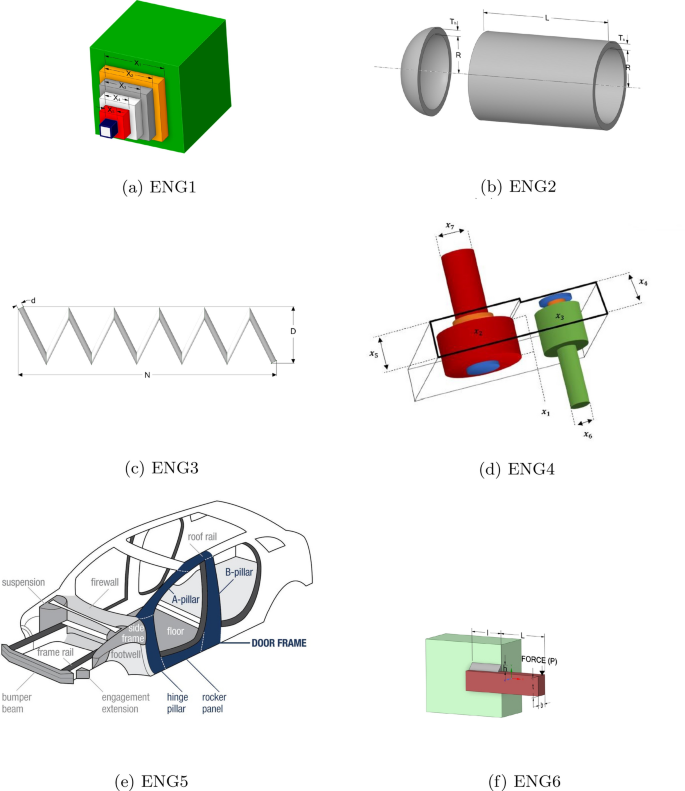

  

  Engineering problems

Here, the convergence performance of DOLFBI for the six engineering problems mentioned above is investigated. It is also interpreted by making comparisons with other pioneering and new metaheuristics. First, the ENG1 (cantilever beam design) results are in Table 10. Accordingly, it can be interpreted that the DOL approach improves FBI, and DOLFBI converges better than other metaheuristics. DOLFBI converges to the smallest (good) value 1.301205963 with [5.951125854, 4.874066596, 4.464381903, 3.478196725, 2.138494389] ideal parameters [42,43,44]. Second, the ENG2 (pressure vessel design) real-world problem is reported in Table 11. Here it can be seen that DOLFBI lags behind FBI by one thousandth, but comes significantly closer compared to other methods. The best cost value of DOLFBI is obtained as 5885.333014, while the ideal parameters calculated are [0.7782, 0.3846, 40.3196, 199.9999] [45]. This method is followed most closely by GWO with 5887.323 value. The third problem, ENG3 (tension/compression spring design), is detailed in Table 12. DOLFBI is the method that gives the best convergence value 0.012665965, followed by HS after FBI. The best cost value of DOLFBI is obtained with the ideal parameters [0.051764678, 0.358539609, 11.18294909]. The fourth problem, ENG4 (speed reducer) result, is reported in Table 13. Here, DOLFBI and FBI have the same convergence performance with the best cost value of 2993.761765. The GOA follows this result with 2994.4245. The fifth is ENG5 (crashworthiness problem), which is more challenging than the others because it is a problem with many parameters and constraints. According to the results in Table 14, it can be interpreted that DOLFBI outperformed FBI, and that the DOL approach improved and improved the FBI significantly but still lagged behind SMO and LIACOR by one thousandth. The best cost value is 22.84298 with SMO, while it is 22.84300988 when DOLFBI is used. Finally, for ENG6 (welded beam design), DOLFBI has lagged behind RSA alone. However, it is seen that it gives more effective results than other compared methods (Table 15).

Table 10 Compared results for cantilever beam design problem

Table 11 Compared results for pressure vessel design problem

Table 12 Compared results for tension/compression spring design problem

Table 13 Compared results for speed reducer problem

Table 14 Compared results for crashworthiness problem

Table 15 Compared results for welded beam design problem

When interpreted in general, it would not be wrong to comment that the DOL approach improves the FBI, although DOLFBI falls in the second and third places in the literature for some challenging problems.

4.4 Truss topology optimization

The arrangement and layout of beam members in a structural system are addressed by structural truss topology. A truss is a frame of triangularly interconnected pieces (such as beams, bars, or rods). The cage’s triangular design provides stability, strength, and stiffness. Truss elements can be assembled in various configurations to meet specific design and engineering needs. The optimization of 20, 24, and 72-bar truss systems is examined in this work. The subheadings provide details on each topology (Table 16).

Table 16 Design parameters of the 20-, 24- and 72-bar truss problems

20-Bar Truss Problem: This structural problem has nine nodes leading to 14 degrees of freedom and is shown in Fig. 10. It is given as a benchmark problem by Kaveh and Zolghadr [46] and Tejani et al. [47]. The design parameters and constraints of the issues are given in Table 16.

Fig. 10

Ground topology structure of 20-truss problem

24-Bar Truss Problem: The second structural problem is 24-bar truss and shown in Fig. 11 and the constraints are given in Table 16.

Fig. 11

Ground topology structure of 24-truss problem

72-Bar Truss Problem: The last truss problem is 72-bar truss has been previously used by Mohan et al. [48]. It has been split into and the constraint size is 198 and these are given in Table 16.

In the 72-bar problem, the elements are clustered in 16 groups. These are C1 (A1−A4), C2 (A5−A12), C3 (A13−A16), C4 (A17−A18), C5 (A19−A22), C6 (A23−A30), C7 (A31−A34), C8 (A35−A36), C9 (A37−A40), C10 (A41−A48), C11 (A49−A52), C12 (A53−A54), C13 (A55−A58), C14 (A59−A66), C15 (A67−A70), and C16 (A71−A72). As it can be seen in Table 12, some clusters (C3 and C16) have been removed for all algorithms and also removed from the Fig. 12.

Fig. 12

Ground topology structure of 72-truss problem

Table 17 compares DOLFBI with the methods in the literature for 24-bar truss topology optimization. Elements less than zero are not taken into account. In addition, the extracted element in all compared methods is not included in the table, for example, 4, 5, 11, 17, 18. Considering the efficient metaheuristic methods in the literature, DOLFBI ranks third. ITLBO takes first place with a minimum weight of 120.0798. However, it can be said that DOLFBI has a competitive convergence behavior. 20-bar truss topology optimization results are reported in Table 18. In this problem, DOLFBI and ITLBO converge to the same and lowest weight values as 154.7988. In this problem, where there are 20 total sections, eight are selected as 1, 5, 8, 11, 13, 15, 18, and 20. Table 19 gives the optimum sections and weights of the 72-bar truss structure. 72-bar truss has a structure that can converge to the optimum weight with few elements. After IOWA, DOLFBI is in second place with 450.388 weight value. The optimum topology of 20 and 24-bar truss problems are given in Fig. 13.

Table 17 Results for the 24-bar truss topology optimization

Table 18 Results for the 20-bar truss topology optimization

Table 19 Results for the 72-bar truss topology optimization

Fig. 13

20 and 24-truss topology optimization with DOLFBI

4.5 Statistical tests

In this study, Wilcoxon sign rank (WSR) and Friedman rank statistical tests are used to show the effectiveness and difference of the proposed method. These two tests are nonparametric statistical tests. The Wilcoxon paired-pairs test is a nonparametric hypothesis test that compares the median of two paired groups and determines whether they are the same distributed [49]. Thus, WSR shows whether there is a significant difference between any two metaheuristic algorithms. In this study, a $5\%$ significance level research is carried out. Friedman rank test determines a rank value for the proposed algorithm [50] (Tables 17, 18, 19).

Table 20 tabulates the WSR results. The p value between DOLFBI and alternative metaheuristic algorithms is displayed in this table. The h value between DOLFBI and methods is 0 for other functions except for FBI in F8 and HBA in F3. This means that DOLFBI differs significantly from the methods compared in the literature. Table 21 reports the Friedman results. According to the Friedman rank results, HGS in F1, HGS, HBA, and AVOA in F19 have the first rank. Considering the function-based rank average of all algorithms, DOLFBI is in the first rank, and then the FBI is in the second rank. In the last ranks, there are SCA and SMA. In CEC2019 and CEC2022 functions, it is clear that DOLFBI precedes other algorithms and exhibits competitive convergence.

Table 20 Wilcoxon sign rank test for benchmark suites

Table 21 Friedman rank test for benchmark suites

4.6 Discussion

The study integrated dynamic oppositional based learning (DOL), an effective population determination method, into one of the newly proposed algorithms, the forensic-based investigation algorithm (FBI). In this case, a more successful convergence was sought by employing DOL, which picks individuals using the opposite approach rather than the original FBI’s random population selection algorithm. With the proposed study, it appears conceivable to improve the convergence outcomes of metaheuristic algorithms, which are regarded to be weak, particularly during the population selection stage.

The paper’s proposed method is compared to basic and enhanced metaheuristic methods. Basic approaches lack the search space’s contrasting strategy. Selecting opposite solution possibilities from the search space reduces the probability of becoming stuck in the local optimum. The enhanced approaches, on the other hand, were likewise developed using the combined opposite selection strategy. However, the FBI exhibits an excellent convergence performance due to the exploitation and exploration capabilities of the Investigation and Pursuit stages.

The impact and contribution of the DOL are evident numerically in the results, especially in the FBI, because two critical population groups are obtained. Additionally, DOLFBI, an enhanced version of FBI, is expected to yield promising results in numerous engineering or challenging real-world scenarios, feature selection with its binary form, and various optimization problems.

5 Conclusions

The DOLFBI presented in this study was created by combining the DOL paradigm with the FBI algorithm. The DOL paradigm, a variant of OBL, promotes efficiency by generating opposing populations and finding the global optimum as quickly and correctly as possible. DOL adaptively and dynamically determines randomly selected populations in traditional FBI for DOLFBI. Unlike primary and complex metaheuristic algorithms, DOLFBI outperforms or lags behind FBI and other algorithms. Twenty-two challenging benchmark problems from CEC2019 and CEC2022 are compared using traditional and sophisticated methodologies.

Compared to standard algorithms, DOLFBI converges to a lower fitness value than other approaches in 18 of 22 benchmark problems (excluding F1, F9, F10, and F22). According to the findings of a comparison with other OBL-based enhanced MAs in the literature, DOLFBI achieved the best convergence for 19 problems except F1, F9, and F22. The Wilcoxon sign and Friedman rank tests validate the results and statistical tests for DOLFBI. Only FBI in the F8 function and $h=0$ in the F3 function in HBA are generated in WSR; in all other circumstances, $h=1$ is generated. According to the Friedman test, DOLFBI ranks top in the CEC2019 and CEC2022 comparison problems. As a result, F4, F10, F14, and F17 demonstrate early convergence behavior. This study also includes a trajectory and qualitative analysis for DOLFBI. The trajectory analysis shows that the oscillation of the first dimension toward the last iteration is fixed and approaches an optimum.

DOLFBI has the best convergence in cantilever beam design, speed reducer, and tension/compression problems in terms of engineering challenges. It is ranked second for welded beam design, third for pressure vessel design, and fourth for crashworthiness.

DOLFBI performs successfully not only in mathematical problems but also in real-world problems. Based on an analysis of the tabulated findings, trajectory analyses, convergence curves, and box-whisker plots, it is evident that DOL yields encouraging outcomes for several FBI improvement issues.

Finally, DOLFBI is employed in the design of 20-, 24-, and 72-bar truss topology optimization challenges. As a result, it is compared to other methods in the literature. The results show that it comes in second position behind TLBO, with an optimal weight of 122.057 at 24-bar. They are on par with ITLBO and in first place with a weight value of 154.7988 at 20 bar. Finally, it ranks second after IWOA for the 72-truss issue, with an optimum value of 450.388.

A binary version of the proposed method can be created and used as a feature selection method in future investigations. Furthermore, the suggested method is adaptable to neural networks, extreme learning machines, and deep learning architectures.

Although dynamic OBL enhances convergence performance, the running time for exploring opposing regions can be computed as O(dim*N). In addition, although this change in running time causes DOLFBI to run slower, this does not cause an extra burden in algorithm complexity. DOLFBI, on the other hand, calls the objective function one last time to maintain the existing optimum value. As a result, the overall number of called functions grows.

Appendix A

See Tables 22, 23, 24.

Table 22 CEC2019 benchmark function problems

Table 23 CEC2022 benchmark function problems

Table 24 Engineering design problems and their properties

References

Head JD, Zerner MC (1989) Newton-based optimization methods for obtaining molecular conformation. In: Advances in quantum chemistry, vol 20, Elsevier, Academic Press, pp 239–290
Liu DC, Nocedal J (1989) On the limited memory bfgs method for large scale optimization. Math Program 45(1–3):503–528
Zeiler MD (2012) Adadelta: an adaptive learning rate method. arXiv preprint arXiv:1212.5701
Duchi J, Hazan E, Singer Y (2011) Adaptive subgradient methods for online learning and stochastic optimization. J Mach Learn Res 12(7):2121–2159
Zhang J (2019) DerivativE−free global optimization algorithms: Population based methods and random search approaches. arXiv preprint arXiv:1904.09368
Hussain K, Salleh MNM, Cheng S, Shi Y (2019) On the exploration and exploitation in popular swarm-based metaheuristic algorithms. Neural Comput Appl 31:7665–7683
Kumar M, Husain D.M, Upreti N, Gupta D (2010) Genetic algorithm: Review and application. Available at SSRN 3529843
Hansen N, Arnold DV, Auger A (2015) Evolution strategies. Springer Handbook of Computational Intelligence, Berlin, pp 871–898
Koza JR et al (1994) Genetic programming, vol 17. MIT Press, Cambridge
Eberhart R, Kennedy J (1995) Particle swarm optimization. In: Proceedings of the IEEE international conference on neural networks, vol 4, Citeseer, pp 1942–1948
Pervaiz S, Ul-Qayyum Z, Bangyal W.H, Gao L, Ahmad J (2021) A systematic literature review on particle swarm optimization techniques for medical diseases detection. Comput Math Methods Med 2021
Bangyal WH, Hameed A, Alosaimi W, Alyami H (2021) A new initialization approach in particle swarm optimization for global optimization problems. Comput Intell Neurosci 2021:1–17
Blum C (2005) Ant colony optimization: introduction and recent trends. Phys Life Rev 2(4):353–373
Karaboga D (2010) Artificial bee colony algorithm. Scholarpedia 5(3):6915
Goffe WL (1996) Simann: a global optimization algorithm using simulated annealing. Stud Nonlinear Dyn Econ. https://doi.org/10.2202/1558-3708.1020
Rashedi E, Nezamabadi-Pour H, Saryazdi S (2009) Gsa: a gravitational search algorithm. Inf Sci 179(13):2232–2248
Hatamlou A (2013) Black hole: a new heuristic optimization approach for data clustering. Inf Sci 222:175–184
Chelouah R, Siarry P (2000) Tabu search applied to global optimization. Eur J Oper Res 123(2):256–270
Zou F, Chen D, Xu Q (2019) A survey of teaching-learning-based optimization. Neurocomputing 335:366–383
Chou J-S, Nguyen N-M (2020) Fbi inspired meta-optimization. Appl Soft Comput 93:106339
Mahdavi S, Rahnamayan S, Deb K (2018) Opposition based learning: a literature review. Swarm Evol Comput 39:1–23
Xu Y, Yang X, Yang Z, Li X, Wang P, Ding R, Liu W (2021) An enhanced differential evolution algorithm with a new oppositional-mutual learning strategy. Neurocomputing 435:162–175
Balande U, Shrimankar D (2022) A modified teaching learning metaheuristic algorithm with oppositE−based learning for permutation flow-shop scheduling problem. Evol Intel 15(1):57–79
Izci D, Ekinci S, Eker E, Dündar A (2021) Improving arithmetic optimization algorithm through modified opposition-based learning mechanism. In: 2021 5th international symposium on multidisciplinary studies and innovative technologies (ISMSIT), IEEE, pp 1–5
Elaziz MA, Abualigah L, Yousri D, Oliva D, Al-Qaness MA, Nadimi-Shahraki MH, Ewees AA, Lu S, Ali Ibrahim R (2021) Boosting atomic orbit search using dynamic-based learning for feature selection. Mathematics 9(21):2786
Shahrouzi M, Barzigar A, Rezazadeh D (2019) Static and dynamic opposition-based learning for colliding bodies optimization. Int J Optim Civil Eng 9(3):499–523
Khaire UM, Dhanalakshmi R, Balakrishnan K, Akila M (2022) Instigating the sailfish optimization algorithm based on opposition-based learning to determine the salient features from a high-dimensional dataset. Int J Informa Technol Decision Making, 1–33
Wang Y, Xiao Y, Guo Y, Li J (2022) Dynamic chaotic opposition-based learning-driven hybrid aquila optimizer and artificial rabbits optimization algorithm: Framework and applications. Processes 10(12):2703
Yildiz BS, Pholdee N, Mehta P, Sait SM, Kumar S, Bureerat S, Yildiz AR (2023) A novel hybrid flow direction optimizer-dynamic oppositional based learning algorithm for solving complex constrained mechanical design problems. Mater Testing 65(1):134–143
Wolpert DH, Macready WG (1997) No free lunch theorems for optimization. IEEE Trans Evol Comput 1(1):67–82
Salet R (2017) Framing in criminal investigation: How police officers (re) construct a crime. Police J 90(2):128–142
Gehl R, Plecas D (2017) Introduction to Criminal Investigation: Processes. Practices and Thinking. Justice Institute of British Columbia, New Westminster-Canada
Xu Y, Yang Z, Li X, Kang H, Yang X (2020) Dynamic opposite learning enhanced teaching-learning-based optimization. Knowl-Based Syst 188:104966
Rahnamayan S, Tizhoosh H.R, Salama M.M (2007) Quasi-oppositional differential evolution. In: 2007 IEEE Congress on Evolutionary Computation, IEEE, pp 2229–2236
Guha D, Roy PK, Banerjee S (2016) Quasi-oppositional differential search algorithm applied to load frequency control. Eng Sci Technol Int J 19(4):1635–1654
Ergezer M, Simon D, Du D (2009) Oppositional biogeography-based optimization. In: 2009 IEEE international conference on systems, man and cybernetics, IEEEE, pp 1009–1014
Sun B, Li W, Huang Y (2022) Performance of composite ppso on single objective bound constrained numerical optimization problems of cec 2022. In: 2022 IEEE congress on evolutionary computation (CEC), IEEE, pp 1–8
Feng Z-K, Niu W-J, Liu S (2021) Cooperation search algorithm: a novel metaheuristic evolutionary intelligence algorithm for numerical optimization and engineering optimization problems. Appl Soft Comput 98:106734
Houssein EH, Saad MR, Hashim FA, Shaban H, Hassaballah M (2020) Lévy flight distribution: a new metaheuristic algorithm for solving engineering optimization problems. Eng Appl Artif Intell 94:103731
Dhiman G (2021) Ssc: a hybrid naturE−inspired meta-heuristic optimization algorithm for engineering applications. Knowl-Based Syst 222:106926
Qais MH, Hasanien HM, Alghuwainem S (2020) Transient search optimization: a new meta-heuristic optimization algorithm. Appl Intell 50(11):3926–3941
Onay FK, Aydemır SB (2022) Chaotic hunger games search optimization algorithm for global optimization and engineering problems. Math Comput Simul 192:514–536
Abualigah L, Elaziz MA, Khasawneh AM, Alshinwan M, Ibrahim RA, Al-qaness MA, Mirjalili S, Sumari P, Gandomi AH (200) Meta-heuristic optimization algorithms for solving real-world mechanical engineering design problems: a comprehensive survey, applications, comparative analysis, and results. Neural Comput Appl, 1–30
Pan J-S, Zhang L-G, Wang R-B, Snášel V, Chu S-C (2022) Gannet optimization algorithm: a new metaheuristic algorithm for solving engineering optimization problems. Math Comput Simul 202:343–373
Zhong C, Li G, Meng Z (2022) Beluga whale optimization: a novel nature-inspired metaheuristic algorithm. Knowled-Based Syst 251:109215
Kaveh A, Zolghadr A (2013) Topology optimization of trusses considering static and dynamic constraints using the css. Appl Soft Comput 13(5):2727–2734
Tejani GG, Savsani VJ, Bureerat S, Patel VK, Savsani P (2019) Topology optimization of truss subjected to static and dynamic constraints by integrating simulated annealing into passing vehicle search algorithms. Eng Comput 35:499–517
Mohan S, Yadav A, Maiti DK, Maity D (2014) A comparative study on crack identification of structures from the changes in natural frequencies using ga and pso. Eng Comput 31(7):1514–1531
Woolson RF (2007) Wilcoxon signed-rank test. Wiley Encyclopedia of Clinical Trials, Hoboken, pp 1–3
Zimmerman DW, Zumbo BD (1993) Relative power of the wilcoxon test, the friedman test, and repeated-measures anova on ranks. J Exp Educat 62(1):75–86
Funding
Open access funding provided by the Scientific and Technological Research Council of Türkiye (TÜBİTAK). Not applicable.
Author information
Authors and Affiliations
Corresponding author
Ethics declarations
Conflict of interest
The author declares that they have no Conflict of interest.
Ethical approval
This article does not contain any studies with human participants performed by any of the authors.
Additional information
Publisher's Note
Springer Nature remains neutral with regard to jurisdictional claims in published maps and institutional affiliations.
Rights and permissions
Open Access This article is licensed under a Creative Commons Attribution 4.0 International License, which permits use, sharing, adaptation, distribution and reproduction in any medium or format, as long as you give appropriate credit to the original author(s) and the source, provide a link to the Creative Commons licence, and indicate if changes were made. The images or other third party material in this article are included in the article's Creative Commons licence, unless indicated otherwise in a credit line to the material. If material is not included in the article's Creative Commons licence and your intended use is not permitted by statutory regulation or exceeds the permitted use, you will need to obtain permission directly from the copyright holder. To view a copy of this licence, visit http://creativecommons.org/licenses/by/4.0/.
About this article
Cite this article
Kutlu Onay, F. Solution of engineering design and truss topology problems with improved forensic-based investigation algorithm based on dynamic oppositional based learning. Neural Comput & Applic (2024). https://doi.org/10.1007/s00521-024-09737-4
Received:
Accepted:
Published:
DOI: https://doi.org/10.1007/s00521-024-09737-4