Connection probabilities of multiple FK-Ising interfaces

Abstract

We find the scaling limits of a general class of boundary-to-boundary connection probabilities and multiple interfaces in the critical planar FK-Ising model, thus verifying predictions from the physics literature. We also discuss conjectural formulas using Coulomb gas integrals for the corresponding quantities in general critical planar random-cluster models with cluster-weight ${q \in [1,4)}$. Thus far, proofs for convergence, including ours, rely on discrete complex analysis techniques and are beyond reach for other values of q than the FK-Ising model ($q=2$). Given the convergence of interfaces, the conjectural formulas for other values of q could be verified similarly with relatively minor technical work. The limit interfaces are variants of $\text {SLE}_\kappa$ curves (with $\kappa = 16/3$ for $q=2$). Their partition functions, that give the connection probabilities, also satisfy properties predicted for correlation functions in conformal field theory (CFT), expected to describe scaling limits of critical random-cluster models. We verify these properties for all $q \in [1,4)$, thus providing further evidence of the expected CFT description of these models.

1 Introduction

Fortuin and Kasteleyn introduced the random-cluster model around the 1970s as a general family of discrete percolation models that combines together Bernoulli percolation, graphical representations of spin models (Ising and Potts models), and polymer models (as a limiting case). Generally in such models, edges are declared to be open or closed according to a given probability measure, the simplest being the independent product measure of Bernoulli percolation. Of particular interest in such models are percolation properties, that is, whether various points in space are connected by paths of open edges. The present article is concerned with boundary-to-boundary connections in the planar case. Such connection events, or crossing events, have been used for a convenient description of the large-scale properties of the Bernoulli percolation model in [38, 66], whereas for dependent percolation models such a description would be much more complex (cf. [66, Question 1.22], see also [22]).

Random-cluster models have been under active research in the past decades, for instance due to their important feature of criticality: for certain parameter values the model exhibits a continuous phase transition. Criticality can be practically identified as follows. Consider on a lattice with small mesh, say $\delta \mathbb {Z}^2$, the probability that an open path connects two opposite sides of a topological rectangle. It is not hard to prove that this probability tends to zero as $\delta \rightarrow 0$ when the model is “subcritical”, while it tends to one as $\delta \rightarrow 0$ when the model is “supercritical”. At the critical point, the connection probability has a nontrivial limit, which is a real number in (0, 1) that depends on the shape (i.e., conformal modulus) of the topological rectangle. This latter fact follows from Russo–Seymour–Welsh type estimates that are now ubiquitous tools for percolation models [12, 20, 24]. Exact identification of the limit of the connection probability, though, is highly non-trivial. Motivated by numerical experiments by Langlands et al. [57], an answer in the physics level of rigor using conformal field theory predictions was given by Cardy for the case of Bernoulli percolation in [9]. The first proof of Cardy’s formula was established by Smirnov [68] using miraculous discrete complex analysis tricks à la Kenyon [47] and Smirnov). To date, analogues and generalizations of Cardy’s formula have been proven only for a number of other models, all of which rely on some kind of specific exact solvability (or “magic”, quoting Smirnov¹), mainly due to underlying free fermion or free boson structures: critical spin-Ising model and FK-Ising model, Gaussian free field, loop-erased random walks, and uniform spanning trees (see [16, 41, 42, 46, 48, 49, 58, 62] and references therein). In the continuum, some connection probabilities for $\text {CLE}$ loops were found in [60], see also [1] for recent results relating to Liouville theory. Analogous numerical results and predictions for connectivity events in the bulk for the random-cluster and Potts models were found in [29].

The phase transition in random-cluster models has been argued to result in conformal invariance and universality for the scaling limit $\delta \rightarrow 0$ of the model (see, e.g., [10]). Since then, tremendous progress has been established towards verifying this prediction. Recently, in [21] it was shown that correlations in the critical random-cluster model with cluster-weight $q \in [1,4]$ do indeed become rotationally invariant in the scaling limit. This provides very strong evidence of conformal invariance, while still not being enough to prove it. For the special case of the FK-Ising model ($q=2$), conformal invariance has been established rigorously to a large extent, thanks to special integrability properties of the model that allow the use of discrete complex analysis in a fundamental way (the “magic” referred to above), cf. [11, 16, 41, 42, 52, 55, 69].

Crucially, in addition to proving conformal invariance, identifying the scaling limit objects with their corresponding counterparts in conformal field theory (CFT) is necessary in order to get access to the full power of the CFT formalism applicable to critical lattice models. The purpose of this article is to provide such an identification for boundary-to-boundary connection probabilities in the FK-Ising model with various boundary conditions (Theorems 1.5 and 1.8). Analogous results remain conjectural for other values² of $q \in [1,4)$. We also provide formulas for the quantities of interest for all $q \in [1,4)$ in terms of solutions to PDE boundary value problems and Coulomb gas integrals, earlier appearing, e.g., in [30, 34, 37]. We also verify CFT predictions for all these formulas (Theorem 1.9), thus providing further evidence for the CFT description of these critical planar models.

Our main results are summarized in Sects. 1.3–1.4. We first discuss the general setup and common terminology for the random-cluster models and the conjectural formulas for the connection probabilities (Sects. 1.1–1.2). Section 1.3 then focuses on results in the special case of the FK-Ising model, and Sect. 1.4 gathers important properties of the Coulomb gas integral formulas in general.

1.1 Random-cluster models in polygons

Here, we summarize notation and terminology to be used throughout, and define the random-cluster model. For more background and properties of these models, we recommend [19, 40].

1.1.1 Notation and terminology

For definiteness, we consider subgraphs $G= (V(G), E(G))$ of the square lattice $\mathbb {Z}^2$, which is the graph with vertex set $V(\mathbb {Z}^2):=\{ z = (m, n) :m, n\in \mathbb {Z}\}$ and edge set $E(\mathbb {Z}^2)$ given by edges between those vertices whose Euclidean distance equals one (called neighbors). This is our primal lattice. Its standard dual lattice is denoted by $(\mathbb {Z}^2)^{\bullet }$. The medial lattice $(\mathbb {Z}^2)^{\diamond }$ is the graph with centers of edges of $\mathbb {Z}^2$ as its vertex set and edges connecting neighbors. For a subgraph $G\subset \mathbb {Z}^2$ (resp. of $(\mathbb {Z}^2)^{\bullet }$ or $(\mathbb {Z}^2)^{\diamond }$), we define its boundary to be the following set of vertices:

$$\begin{aligned} \partial G= \{ z \in V(G) \, :\, \exists \; w \not \in V(G) \text { such that }\langle z,w \rangle \in E(\mathbb {Z}^2)\} . \end{aligned}$$

When we add the subscript or superscript $\delta$, we mean that subgraphs of the lattices $\mathbb {Z}^2, (\mathbb {Z}^2)^{\bullet }, (\mathbb {Z}^2)^\diamond$ have been scaled by $\delta > 0$. We consider the models in the scaling limit $\delta \rightarrow 0$. For a given medial graph $\Omega ^{\delta , \diamond } \subset (\delta \mathbb {Z}^2)^{\diamond }$, let $\Omega ^{\delta }\subset \delta \mathbb {Z}^2$ be the graph on the primal lattice corresponding to $\Omega ^{\delta , \diamond }$ (see details in Sect. 3.1). By a (discrete) polygon we either refer to the medial graph $\Omega ^{\delta , \diamond }$ endowed with given distinct boundary points $x_1^{\delta , \diamond }, \ldots , x_{2N}^{\delta , \diamond }$ in counterclockwise order, or to the corresponding primal graph $(\Omega ^{\delta }; x_1^{\delta }, \ldots , x_{2N}^{\delta })$ with given boundary points $x_1^{\delta }, \ldots , x_{2N}^{\delta }$ in counterclockwise order. We consider random-cluster models on such polygons, where the boundary behavior changes at the marked boundary points.

1.1.2 Random-cluster model

Let $G= (V(G), E(G))$ be a finite subgraph of $\mathbb {Z}^2$. A random-cluster configuration $\omega =(\omega _e)_{e \in E(G)}$ is an element of $\{0,1\}^{E(G)}$. An edge $e \in E(G)$ is said to be open (resp. closed) if $\omega _e=1$ (resp. $\omega _e=0$). We view the configuration $\omega$ as a subgraph of $G$ with vertex set $V(G)$ and edge set $\{e\in E(G) :\omega _e=1\}$. We denote by $o(\omega )$ (resp. $c(\omega )$) the number of open (resp. closed) edges in $\omega$.

We are interested in the connectivity properties of the graph $\omega$ with various boundary conditions. The maximal connected³ components of $\omega$ are called clusters. The boundary conditions encode how the vertices are connected outside of $G$. Precisely, by a boundary condition $\pi$ we refer to a partition $\pi _1 \sqcup \cdots \sqcup \pi _m$ of the boundary $\partial G$. Two vertices $z,w \in \partial G$ are said to be wired in $\pi$ if $z,w \in \pi _j$ for some common j. In contrast, free boundary segments comprise vertices that are not wired with any other vertex (so the corresponding part $\pi _j$ is a singleton). We denote by $\omega ^{\pi }$ the (quotient) graph obtained from the configuration $\omega$ by identifying the wired vertices in $\pi$.

Finally, the random-cluster model on $G$ with edge-weight $p\in [0,1]$, cluster-weight $q>0$, and boundary condition $\pi$, is the probability measure $\smash {\mu ^{\pi }_{p,q,G}}$ on the set $\{0,1\}^{E(G)}$ of configurations $\omega$ defined by

$$\begin{aligned} \mu ^{\pi }_{p,q,G}[\omega ] := \;&\frac{p^{o(\omega )}(1-p)^{c(\omega )}q^{k(\omega ^{\pi })}}{\sum _{\varpi \in \{0,1\}^{E(G)}} p^{o(\varpi )}(1-p)^{c(\varpi )}q^{k(\varpi ^{\pi })} } , \end{aligned}$$

where $k(\omega ^{\pi })$ is the number of connected components of the graph $\omega ^{\pi }$. For $q=2$, this model is also known as the FK-Ising model, while for $q=1$, it is simply the Bernoulli bond percolation (assigning independent values for each $\omega _e$). The random-cluster model combines together several important models in the same family. For integer values of q, it is very closely related to the q-Potts model, and by taking a suitable limit, the case of $q=0$ corresponds to the uniform spanning tree (see, e.g., [19]). It has been proven for the range $q \in [1,4]$ in [24] that when the edge-weight is chosen suitably, namely as (the critical, self-dual value)

$$\begin{aligned} p = p_c(q) := \frac{\sqrt{q}}{1+\sqrt{q}} , \end{aligned}$$

(1.1)

Fig. 1

Consider discrete polygons (gray) with six marked boundary points. One possible boundary condition for the random-cluster model is illustrated in the left figure, where the arcs $(x_1 \, x_2), (x_3 \, x_4), (x_5 \, x_6)$ are wired, and the arcs $(x_1 \, x_2)$ and $(x_5 \, x_6)$ are further wired outside of the polygon. This boundary condition corresponds to the non-crossing partition $\{\{1,3\}, \{2\}\}$ of the three wired boundary arcs. One possible random-cluster configuration in terms of its loop representation is illustrated in the right figure. It comprises loops (black) and three interfaces inside the polygon: the orange curve connects $x_1^{\diamond }$ and $x_{2}^{\diamond }$; the purple curve connects $x_3^{\diamond }$ and $x_6^{\diamond }$; and the green curve connects $x_4^{\diamond }$ and $x_5^{\diamond }$. See Sect. 3 for details (color figure online)

then the random-cluster model exhibits a continuous phase transition in the sense that after taking the infinite-volume (thermodynamic) limit, for $p > p_c(q)$ there almost surely exists an infinite cluster, while for $p < p_c(q)$ there does not, and the limit $p \searrow p_c(q)$ is approached in a continuous way. (This is also expected to hold when $q \in (0,1)$, while it is known that the phase transition is discontinuous when $q > 4$ by [25].) Therefore, the scaling limit of the model at its critical point (1.1) is expected to be conformally invariant for all $q \in [0,4]$. In the present article, we will consider multiple interfaces and boundary-to-boundary connection probabilities in the critical random-cluster model with $q \in [1,4)$. See also [58] for the uniform spanning tree model corresponding to $q=0$.

1.1.3 Markov property

At the heart of many geometric arguments concerning the random-cluster model is its (domain) Markov property: the restriction of the model to a smaller graph only depends on the boundary condition induced by such a restriction. To state this more precisely, fix any $p\in [0,1]$ and $q>0$, and suppose that $G\subset G'$ are two finite subgraphs of $\mathbb {Z}^2$ and that we have fixed a boundary condition $\pi$ for the model on the boundary $\partial G'$ of the larger graph. Let X be a random variable which is measurable with respect to the status of the edges in the smaller graph $G$. Then, for all $\upsilon \in \{0,1\}^{E(G'){\setminus } E(G)}$, we have

$$\begin{aligned} \mu ^{\pi }_{p,q,G'} \big [X \; | \; \omega _e = \upsilon _e \text { for all } e \in E(G'){\setminus } E(G)\big ] = \mu ^{\upsilon ^{\pi }}_{p,q,G}[X], \end{aligned}$$

where $\upsilon ^{\pi }$ is the partition on $\partial G$ obtained by wiring two vertices in $\partial G$ if they are connected in $\upsilon$. For instance, taking $G$ to be a connected component of the complement of the purple curve in Fig. 1, we obtain a random-cluster model on the smaller graph $G$ with modified boundary conditions.

1.1.4 Boundary conditions

Consider now the random-cluster model on a polygon $(\Omega ^{\delta }; x_1^{\delta }, \ldots , x_{2N}^{\delta })$ with the following boundary conditions: first, every other boundary arc is wired,

$$\begin{aligned} (x_{2r-1}^{\delta } \, x_{2r}^{\delta }) \text { is wired,} \quad \text {for all}\quad r \in \{1,2,\ldots , N\} , \end{aligned}$$

and second, these N wired arcs are further wired together according to a non-crossing partition $\pi$ outside of $\Omega ^{\delta }$, as illustrated in Figs. 1 and 2. Note that there is a natural bijection $\beta \leftrightarrow \pi _\beta$ between non-crossing partitions $\pi _\beta$ of the N wired boundary arcs and planar link patterns $\beta$ with N links,

$$\begin{aligned} \beta =&\{ \{a_1,b_1\}, \{a_2,b_2\},\ldots , \{a_N,b_N\}\} \nonumber \\&\text {with link endpoints ordered as } \; a_1< a_2< \cdots< a_N\quad \text {and}\quad a_r< b_r ,\nonumber \\&\text {for all}\quad 1 \le r \le N , \nonumber \\&\text {and such that there are no indices } 1 \le r , s \le N \quad \text {with}\quad a_r< a_s< b_r < b_s , \end{aligned}$$

(1.2)

where $\{a_1, b_1, \ldots , a_N, b_N\}=\{1,2, \ldots , 2N\}$ and the pairs $\{a_j,b_j\}$ are called links. Hence, we encode the boundary condition $\pi _\beta$ in a label $\beta$. We denote by $\text {LP}_N \ni \beta$ the set of planar link patterns of N links.

Fig. 2

Consider discrete polygons with six marked points on the boundary. One possible boundary condition for the random-cluster model is illustrated in a. The corresponding possible planar link patterns $\alpha$ formed by the interfaces are depicted in red in b(bottom), and they correspond to non-crossing partitions inside b(top)

Let $\omega$ be a critical random-cluster configuration on $\Omega ^{\delta }$ with boundary condition $\beta$. For notational ease, keeping $q \in [1,4)$ and $p = p_c(q)$ fixed, we denote its law by

$$\begin{aligned} \mathbb {P}_{\beta }^{\delta } := \mu ^{\pi _{\beta }}_{p_c(q),q,\Omega ^{\delta }} . \end{aligned}$$

We consider in particular the cluster boundaries of $\omega$ (that is, its loop representation, see Fig. 1 and Sect. 3). By planarity, there exist N curves, interfaces, on the medial graph $\Omega ^{\delta , \diamond }$ running along $\omega$ and connecting the marked points $\{x_1^{\delta , \diamond }, x_2^{\delta , \diamond },\ldots , x_{2N}^{\delta , \diamond }\}$ pairwise, as also illustrated in Fig. 1. Let us denote by $\vartheta _{\textrm{RCM}}^{\delta }$ the random planar connectivity in $\text {LP}_N$ formed by the N discrete interfaces. In this article, we are particularly interested in the connection probabilities $\smash {\mathbb {P}_{\beta }^{\delta }}[\vartheta _{\textrm{RCM}}^{\delta }=\alpha ]$ for $\alpha \in \text {LP}_N$, as functions of the marked boundary points—Fig. 2 illustrates these crossing events. The goal is to study conjectures for the scaling limits of the interfaces and their connection probabilities, and prove these conjectures for the case of the critical FK-Ising model (which has $q=2$ and $p = p_c(2) = \frac{\sqrt{2}}{1+\sqrt{2}}$).

1.1.5 Scaling limits

To specify in which sense the convergence as $\delta \rightarrow 0$ should take place, we need a notion of convergence of polygons. In contrast to the commonly used Carathéodory convergence of planar sets, we need a slightly stronger notion termed close-Carathéodory convergence, following Karrila [44]. The precise definition will be given in Sect. 3.1 (Definition 3.1). Roughly speaking, the usual Carathéodory convergence allows wild behavior of the boundary approximations, while in order to obtain tightness of the random interfaces (i.e., precompactness needed to find convergent subsequences), a slightly stronger convergence which guarantees good approximations around the marked boundary points is required.

We also need a topology for the interfaces, which we regard as (images of) continuous mappings from [0, 1] to $\mathbb {C}$ modulo reparameterization (i.e., planar oriented curves). For a simply connected domain $\Omega \subsetneq \mathbb {C}$, we will consider curves in $\overline{\Omega }$. For definiteness, we map $\Omega$ onto the unit disc $\mathbb {U}:= \{ z \in \mathbb {C}:|z| < 1 \}$: for this we shall fix⁴ any conformal map $\Phi$ from $\Omega$ onto $\mathbb {U}$. Then, we endow the curves with the metric

$$\begin{aligned} \text {dist}(\eta _1, \eta _2) := \inf _{\psi _1, \psi _2} \sup _{t\in [0,1]} |\Phi (\eta _1(\psi _1(t)))-\Phi (\eta _2(\psi _2(t)))| , \end{aligned}$$

(1.3)

where the infimum is taken over all increasing homeomorphisms $\psi _1, \psi _2 :[0,1]\rightarrow [0,1]$. The space of continuous curves on $\overline{\Omega }$ modulo reparameterizations then becomes a complete separable metric space.

1.1.6 Loewner chains

To describe scaling limits of interfaces, we recall that planar chordal curves can be dynamically generated by Loewner evolution. In general, any continuous real-valued function, called the driving function $W_t :[0,\infty ) \rightarrow \mathbb {R}$, gives rise to a growing family of sets via the following recipe (see [56, 65] for background). The Loewner equation

$$\begin{aligned} \partial _{t}{g}_{t}(z) = \frac{2}{g_{t}(z)-W_{t}} , \quad \text {with initial condition} \quad g_{0}(z)=z , \end{aligned}$$

(1.4)

is an ordinary differential equation in time $t \ge 0$, for each fixed point in the upper half-plane, $z \in \mathbb {H}:= \{ z \in \mathbb {C}:{\text {Im}}(z) > 0 \}$. It has a unique solution $(g_{t}, t\ge 0)$ up to $T_{z}:= \sup \{t\ge 0 :\min _{s\in [0,t]} |g_{s}(z)-W_{s}|>0\}$, called the swallowing time of z. The Loewner chain is a dynamical family of conformal bijections⁵$g_{t} :\mathbb {H}{\setminus } K_{t} \rightarrow \mathbb {H}$, where the hull of swallowed points is $K_{t}:=\overline{\{z\in \mathbb {H}:T_{z}\le t\}}$. We also say that the Loewner chain is parameterized by half-plane capacity, which refers to the property that for each time $t \ge 0$, the coefficient of $z^{-1}$ in the series expansion of $g_t$ at infinity equals 2t (this coefficient is, by definition, the half-plane capacity of the hull $K_{t}$, measuring its size as seen from infinity).

The family $(K_{t}, t\ge 0)$ of hulls is also often called a Loewner chain, and it is said to be generated by a continuous curve $\eta :[0,T) \rightarrow \overline{\mathbb {H}}$ if for each $t \in [0,T)$, the set $\mathbb {H}{\setminus } K_{t}$ is the unbounded connected component of $\mathbb {H}{\setminus } \eta [0,t]$. We also refer to the curve $\eta$ as a Loewner chain. An example of a Loewner chain generated by a continuous curve is the chordal Schramm–Loewner evolution, $\text {SLE}_{\kappa }$, that is the random Loewner chain driven by $W = \sqrt{\kappa } \, B$, a standard one-dimensional Brownian motion B of speed $\kappa > 0$. This family indexed by $\kappa$ is uniquely determined by the following two properties.

• Conformal invariance: The law of the $\text {SLE}_{\kappa }$ curve $\eta$ in any simply connected domain $\Omega$ is the pushforward of the law of the $\text {SLE}_{\kappa }$ curve in $\mathbb {H}$ by a conformal map $\varphi :\mathbb {H}\rightarrow \Omega$ which maps the two points $0, \infty$ to the two endpoints of $\eta$.

• Domain Markov property: given a stopping time $\tau$ and initial segment $\eta [0,\tau ]$ of the $\text {SLE}_\kappa$ curve in $\mathbb {H}$, the conditional law of the remaining piece $\eta [\tau ,\infty )$ is the law of the $\text {SLE}_\kappa$ curve from the tip $\eta (\tau )$ to $\infty$ in the unbounded connected component of $\mathbb {H}{\setminus } \eta [0,\tau ]$.

The standard $\text {SLE}_\kappa$ curve in $\mathbb {H}$ connects the two boundary points $0 = \eta (0)$ and $\infty = \lim _{t \rightarrow \infty } |\eta (t)|$. One can change the target point by adding a specific drift to the driving Brownian motion (corresponding to the case $N=1$ in Theorem 1.5 when $\kappa = 16/3$). The parameter $\kappa > 0$ describes the behavior and the fractal dimension of the $\text {SLE}_\kappa$ curve. For instance, it is almost surely a simple curve when $\kappa \le 4$, while for $\kappa \ge 8$, the $\text {SLE}_\kappa$ curve is almost surely space-filling. In the intermediate parameter range $\kappa \in (4,8)$, including the parameter range considered in the present article, the $\text {SLE}_\kappa$ curve almost surely has self-touchings, but is not space-filling. See [56, 65] for background and further properties of this process.

1.2 Conjectures for random-cluster models

Let us now fix parameters

$$\begin{aligned} \kappa \in (4,8) , \quad h(\kappa ) := \frac{6-\kappa }{2\kappa } , \quad \text {and} \quad q(\kappa ) := 4\cos ^2(4\pi /\kappa ) . \end{aligned}$$

Note that when $\kappa \in (4,6]$, we have $q = q(\kappa ) \in [1,4)$ corresponding to the critical random-cluster model with $p = p_c(q)$. (The case of $\kappa = 4$ corresponds to $q = 4$, which is still critical. We comment on this case in Remark 1.12.) To state the expected formulas describing the scaling limits of multiple interfaces and connection probabilities in the critical random-cluster models, we define for each $\beta \in \text {LP}_N$ the basis Coulomb gas integral functions⁶ as

(1.5)

where the integration contours are pairwise non-intersecting paths in the upper half-plane connecting the marked points pairwise according to the connectivity $\beta$, and the integrand is

$$\begin{aligned} f (\varvec{x};u_1,\ldots ,u_N)&:= \prod _{1\le i<j\le 2N}(x_{j}-x_{i})^{2/\kappa } \prod _{1\le r<s\le N}(u_{s}-u_{r})^{8/\kappa } \nonumber \\&\quad \times \prod _{\begin{array}{c} 1\le i\le 2N \\ 1\le r\le N \end{array}} (u_{r}-x_{i})^{-4/\kappa } , \end{aligned}$$

(1.6)

and the branch of this multivalued integrand is chosen to be real and positive when

$$\begin{aligned} x_{a_r}< {\text {Re}}(u_r) < x_{a_r+1} , \quad \text {for all}\quad 1 \le r \le N . \end{aligned}$$

In (1.5), we use the integration symbols to indicate that the integration of the variable $u_r$ is performed from $x_{a_r}$ to $x_{b_r}$ in the upper half-plane. Formulas of type (1.5), while originating from the Coulomb gas formalism of conformal field theory [26, 51], have appeared in the $\text {SLE}$ literature [30, 31, 50] as partition functions for $\text {SLE}_\kappa$ variants, and have then been used in the physics literature [34, 37] pertaining to Conjecture 1.3. Our formulas are motivated by their properties listed in Theorem 1.9. In particular, $\mathcal {G}_{\beta }$ are indeed partition functions of multiple $\text {SLE}_\kappa$ curves.

For fixed $N\ge 1$, by a polygon $(\Omega ; x_1, \ldots , x_{2N})$ we refer to a bounded simply connected domain $\Omega \subset \mathbb {C}$ with distinct marked boundary points $x_1, \ldots , x_{2N} \in \partial \Omega$ in counterclockwise order, such that $\partial \Omega$ is locally connected. We extend the definition of $\mathcal {G}_{\beta }$ to a general polygon $(\Omega ; x_1, \ldots , x_{2N})$ whose marked boundary points $x_1, \ldots , x_{2N}$ lie on sufficiently regular boundary segments (e.g., $C^{1+\epsilon }$ for some $\epsilon >0$) as

$$\begin{aligned} \mathcal {G}_{\beta }(\Omega ; x_1, \ldots , x_{2N}) := \prod _{j=1}^{2N} |\varphi '(x_j)|^{h(\kappa )} \times \mathcal {G}_{\beta }(\varphi (x_1), \ldots , \varphi (x_{2N})) , \end{aligned}$$

(1.7)

where $\varphi$ is any conformal map from $\Omega$ onto $\mathbb {H}$ with $\varphi (x_1)<\cdots <\varphi (x_{2N})$. It follows from the Möbius covariance (1.12) in Theorem 1.9 that this definition is independent of the choice of the map $\varphi$.

We formulate the next Conjectures 1.1 and 1.3 in the case of square-lattice approximations, which is the setup that we use to give detailed proofs of these conjectures for the critical FK-Ising model in Theorems 1.5 and 1.8. By universality, we expect the same results to hold with any approximations. In fact, one should be able to readily extend Theorems 1.5 and 1.8 to more general discrete approximations following the lines of [16, 18]. For the sake of presentation, we content ourselves in the present work to the simplest setup.

Conjecture 1.1

Fix a polygon $(\Omega ; x_1, \ldots , x_{2N})$ and a link pattern $\beta \in \text {LP}_N$. Suppose that a sequence $(\Omega ^{\delta , \diamond }; x_1^{\delta , \diamond }, \ldots , x_{2N}^{\delta , \diamond })$ of medial polygons converges to $(\Omega ; x_1, \ldots , x_{2N})$ in the close-Carathéodory sense (as detailed in Definition 3.1). Consider the critical random-cluster model with cluster-weight $q \in [1,4)$ on the primal polygon $(\Omega ^{\delta }; x_1^{\delta }, \ldots , x_{2N}^{\delta })$ with boundary condition $\beta$. For each $i\in \{1,2,\ldots , 2N\}$, let $\eta _i^{\delta }$ be the interface starting from the boundary point $x_i^{\delta , \diamond }$. Let $\varphi$ be any conformal map from $\Omega$ onto $\mathbb {H}$ such that $\varphi (x_1)<\cdots <\varphi (x_{2N})$. Then, $\eta _i^{\delta }$ converges weakly to the image under $\varphi ^{-1}$ of the Loewner chain with the following driving function, up to the first time when $\varphi (x_{i-1})$ or $\varphi (x_{i+1})$ is swallowed:

$$\begin{aligned} {\left\{ \begin{array}{ll} \text {d}W_t = \sqrt{\kappa } \, \text {d}B_t + \kappa (\partial _i\log \mathcal {G}_{\beta })\left( V_t^{1}, \ldots , V_t^{i-1}, W_t, V_t^{i+1}, \ldots , V_t^{2N}\right) \, \text {d}t, \\ \text {d}V_t^j =\frac{2 \, \text {d}t}{V_t^j-W_t},\\ W_0=\varphi (x_i),\\ V_0^j=\varphi (x_j),\quad j\in \{1,\ldots , i-1, i+1, \ldots , 2N\}, \end{array}\right. } \end{aligned}$$

(1.8)

where $\mathcal {G}_{\beta }$ is defined in (1.5).

We prove Conjecture 1.1 for $q=2$ in Theorem 1.5.

Definition 1.2

A meander formed from two link patterns $\alpha ,\beta \in \text {LP}_N$ is the planar diagram obtained by placing $\alpha$ and the horizontal reflection $\beta$ on top of each other. We denote by $\mathcal {L}_{\alpha ,\beta }$ the number of loops in the meander formed from $\alpha$ and $\beta$. We define the meander matrix $\{\mathcal {M}_{\alpha , \beta }(q(\kappa )) :\alpha ,\beta \in \text {LP}_N\}$ via

$$\begin{aligned} \mathcal {M}_{\alpha ,\beta }(q(\kappa )) := \sqrt{q(\kappa )}^{\; \mathcal {L}_{\alpha ,\beta }}. \end{aligned}$$

(1.9)

An example of a meander is

Conjecture 1.3

Assume the same setup as in Conjecture 1.1. The endpoints of the N interfaces give rise to a random planar link pattern $\vartheta _{\textrm{RCM}}^{\delta }$ in $\text {LP}_N$. For any $\alpha \in \text {LP}_N$, we have

$$\begin{aligned} \lim _{\delta \rightarrow 0}\mathbb {P}_{\beta }^{\delta }[\vartheta _{\textrm{RCM}}^{\delta }=\alpha ] \; = \; \mathcal {M}_{\alpha ,\beta }(q(\kappa )) \; \frac{\mathcal {Z}_{\alpha }(\Omega ; x_1, \ldots , x_{2N})}{\mathcal {G}_{\beta }(\Omega ; x_1, \ldots , x_{2N})}, \end{aligned}$$

(1.10)

where $\mathcal {G}_{\beta }$ and $\mathcal {M}_{\alpha ,\beta }$ are defined in (1.5, 1.7) and (1.9), respectively, and $\{\mathcal {Z}_{\alpha } :\alpha \in \text {LP}_N\}$ is the collection of pure partition functions for multiple $\text {SLE}_{\kappa }$ described in Definition 1.4 below.

We prove Conjecture 1.3 for $q=2$ in Theorem 1.8.

The content of Conjectures 1.1 and 1.3 has been predicted in the physics literature and also numerically verified in some cases with high precision, see [36, 37] and references therein. Via a similar strategy as in the proof of Theorem 2.7, by using Theorem 2.6 one can verify that our formula (1.5) for $\mathcal {G}_\beta$ is consistent with the prediction in [37, Eq. (11)].

“Pure partition functions” refer to a family of smooth functions defined as solutions to a system of partial differential equations (PDEs) important in both CFT and SLE theory, with certain recursive asymptotic boundary conditions. Uniqueness results for solutions to PDEs are usually not available. However, it was proven by Flores and Kleban [32, 33] that in this particular case, we do have a classification if we impose certain additional requirements (covariance (COV) and growth bound (PLB)). The PDEs appear in the pioneering CFT articles [6, 7] of Belavin, Polyakov, and Zamolodchikov (BPZ) as a feature of the algebraic structure of conformal symmetry for certain fields, and in early articles in SLE theory by Bauer et al. [3], and Dubédat [30, 31], as a manifestation of certain martingales.

• (PDE) BPZ equations: for all $j\in \{1,\ldots ,2N\}$,

  $$\begin{aligned} \bigg [ \frac{\kappa }{2}\frac{\partial ^{2}}{\partial x_{j}^{2}} + \sum _{i \ne j} \Big ( \frac{2}{x_{i}-x_{j}} \frac{\partial }{\partial x_{i}} - \frac{2h(\kappa )}{(x_{i}-x_{j})^{2}} \Big ) \bigg ] F(x_1,\ldots ,x_{2N}) = 0. \end{aligned}$$

  (1.11)

The covariance gives a version of global conformal symmetry for the functions.

• (COV) Möbius covariance: for all Möbius maps $\varphi$ of the upper half-plane $\mathbb {H}$ such that $\varphi (x_{1})< \cdots < \varphi (x_{2N})$,

  $$\begin{aligned} F(x_{1},\ldots ,x_{2N}) = \prod _{i=1}^{2N} \varphi '(x_{i})^{h(\kappa )} \times F(\varphi (x_{1}),\ldots ,\varphi (x_{2N})). \end{aligned}$$

  (1.12)

Definition 1.4

Fix $\kappa \in (0,6]$. The pure partition functions of multiple $\text {SLE}_{\kappa }$ are the recursive collection $\{\mathcal {Z}_{\alpha } :\alpha \in \bigsqcup _{N\ge 0} \text {LP}_N\}$ of functions $\mathcal {Z}_{\alpha } :\mathfrak {X}_{2N}\rightarrow \mathbb {R}_{>0}$ uniquely determined by the following properties. They satisfy the PDE system (1.11), Möbius covariance (1.12), as well as (ASY) and (PLB) given below.

• (ASY) Asymptotics: With $\mathcal {Z}_{\emptyset } \equiv 1$ for the empty link pattern $\emptyset \in \text {LP}_0$, the collection $\{\mathcal {Z}_{\alpha } :\alpha \in \text {LP}_N\}$ satisfies the following recursive asymptotics property. Fix $N \ge 1$ and $j \in \{1,2, \ldots , 2N-1 \}$. Then, we have

  $$\begin{aligned} \;&\lim _{x_j,x_{j+1}\rightarrow \xi } \frac{\mathcal {Z}_{\alpha }(\varvec{x})}{ (x_{j+1}-x_j)^{-2h(\kappa )} } = {\left\{ \begin{array}{ll} \mathcal {Z}_{\alpha /\{j,j+1\}}(\varvec{\ddot{x}}_j), &{} \text {if}\quad \{j, j+1\}\in \alpha , \\ 0 , &{} \text {if}\quad \{j, j+1\} \not \in \alpha , \end{array}\right. } \end{aligned}$$

  (1.13)

  where

  $$\begin{aligned} \begin{aligned} \varvec{x} = \;&(x_1, \ldots , x_{2N}) \in \mathfrak {X}_{2N} , \\ \varvec{\ddot{x}}_j = \;&(x_1, \ldots , x_{j-1}, x_{j+2}, \ldots , x_{2N}) \in \mathfrak {X}_{2N-2} , \end{aligned} \end{aligned}$$

  (1.14)

  and $\xi \in (x_{j-1}, x_{j+2})$ (with the convention that $x_0 = -\infty$ and $x_{2N+1} = +\infty$).

• (PLB) The functions are positive and satisfy the power-law bound

  $$\begin{aligned} 0<\mathcal {Z}_{\alpha }(\varvec{x})\le \prod _{\{a,b\}\in \alpha }|x_b-x_a|^{-2h(\kappa )}, \quad \text {for all}\quad \varvec{x}\in \mathfrak {X}_{2N} . \end{aligned}$$

  (1.15)

We extend the definition of $\mathcal {Z}_{\alpha }$ to more general polygons $(\Omega ; x_1, \ldots , x_{2N})$ as in (1.7) (replacing $\mathcal {G}_{\beta }$ by $\mathcal {Z}_{\alpha }$).

With a weaker power-law bound and relaxing the positivity requirement in (1.15), the collection $\{\mathcal {Z}_{\alpha } :\alpha \in \text {LP}_N\}$ was first constructed in [33] indirectly by using Coulomb gas integrals for all $\kappa \in (0,8)$, and explicitly for all $\kappa \in (0,8) {\setminus } \mathbb {Q}$ in [50], following the conjectures from [3]. It is believed that these functions satisfy (1.15) for all $\kappa \in (0,8)$. In general, for the range $\kappa \in (0,8]$, to our knowledge there are explicit formulas for $\mathcal {Z}_{\alpha }$ only when $\kappa \notin \mathbb {Q}$ (cf. [50]) and for a few special rational cases: $\kappa = 2$ [48]; $\kappa =4$ [62]; and $\kappa =8$ [58]. For $\kappa \in (0,6]$, an explicit probabilistic construction was given in [70, Theorem 1.7], which immediately implies (1.15). See also Remark 1.11 and [63].

1.3 Results: multiple interfaces and connection probabilities for the FK-Ising model

Our first main result concerns the scaling limit of the FK-Ising interfaces.

Theorem 1.5

Conjecture 1.1 holds for $q=2$ and $\kappa =16/3$. In this case, we have

$$\begin{aligned} \mathcal {G}_\beta (x_1, \ldots , x_{2N}) = \;&\mathcal {F}_{\beta } (x_1, \ldots , x_{2N}) \nonumber \\ := \;&\prod _{s=1}^N |x_{b_s}-x_{a_s}|^{-1/8}\nonumber \\&\left( \sum _{\varvec{\sigma } \in \{\pm 1\}^N}\prod _{1\le s < t \le N} \chi (x_{a_s}, x_{a_t}, x_{b_t}, x_{b_s})^{\sigma _s \sigma _t / 4}\right) ^{1/2} , \end{aligned}$$

(1.16)

where $\varvec{\sigma } = (\sigma _1, \sigma _2, \ldots , \sigma _N)\in \{\pm 1\}^N$ and $\chi :\mathbb {R}^4\rightarrow \mathbb {R}$ is the cross-ratio

$$\begin{aligned} \chi _{1,2,3,4} = \chi (y_1, y_2, y_3, y_4):= \frac{|y_2-y_1| \, |y_4-y_3|}{|y_3-y_1| \, |y_4-y_2|} . \end{aligned}$$

(1.17)

Remark 1.6

The square of this formula also appears in moments of the real part of an imaginary Gaussian multiplicative chaos distribution [43, Theorem 1.5].

The case $N=1$ of one curve in Theorem 1.5 was proven in a celebrated group effort summarized in [11]. The scaling limit curve is the chordal Schramm–Loewner evolution. The proof in the case of $N=1$ involves two main steps. The first step is to show that the sequence $\{\eta _1^{\delta }\}_{\delta >0}$ of interfaces is tight, which implies precompactness by Prokhorov’s theorem, and thus enables finding convergent subsequences $\eta _1^{\delta _n} \rightarrow \eta _1$ with some limit curve $\eta _1$. Second, one has to show that all of these subsequences actually converge to the same limit, identified in this case with the chordal $\text {SLE}_{16/3}$. The precompactness step is established by refined crossing estimates [20, 53], while the identification of the limit curve involves an ingenious usage of a discrete holomorphic spinor observable (devised by Smirnov [69] and further developed by Chelkak, Smirnov, and others, cf. [13, 14, 16]) converging to its continuum counterpart, which gives the sought driving function $W_t = \sqrt{16/3} \, B_t$ via a suitable series expansion.

In the case $N=2$ of two curves $(\eta _1,\eta _2)$, Theorem 1.5 was proven in [16, 54]. Since the conformal invariance fixes three real degrees of freedom, while the polygon $(\Omega ; x_1, x_2, x_3, x_4)$ has four real degrees of freedom, a similar strategy as in the case of one curve gives the result, and the driving function of one curve, say $\eta _1$ (in its marginal law), is given by Brownian motion with a drift involving the hypergeometric function. Essentially, the only additional input compared to the case of $N=1$ is that one has to solve an ordinary differential equation for the drift term, which results in the hypergeometric equation.

The case of $N \ge 3$ is significantly more involved. Because there are several degrees of freedom, the identification of the scaling limit requires finding a suitable multi-point discrete holomorphic spinor observable, or alternatively, some other proof strategy. For the special case where the boundary condition is the totally unnested link pattern

$$\begin{aligned} \beta = \varvec{\underline{\cap \cap }}:= \{\{1,2\} , \{3,4\} , \ldots , \{2N-1, 2N\}\} , \end{aligned}$$

(1.18)

Theorem 1.5 was proven recently by Izyurov [42] and earlier implicitly conjectured by Flores et al. [37]. In Sect. 3, we will prove Theorem 1.5 with general boundary conditions $\beta$. The main addition compared to the earlier results is the identification of the drift term for general $\beta$, given by (1.16), and finding a suitably general multi-point observable. The rough strategy is the following.

• We construct a discrete holomorphic observable with general boundary conditions in Sect. 3.2 and identify its scaling limit observable $\phi _{\beta }$ in Sect. 3.4. This is a generalization of the previous observables constructed in [16, 41, 42]. Some key ideas for the proof in Sect. 3.4 are learned from [41].

• We analyze the observable $\phi _{\beta }$, expand it to certain precision, and relate its expansion coefficients to $\mathcal {F}_{\beta }$ in Sect. 3.3. This step is rather technical, but contains the gist of the proof of Theorem 1.5: identification of the scaling limit (1.8) with the explicit drift given by the function $\mathcal {F}_{\beta }$ in formula (1.16). The form of the function $\mathcal {F}_{\beta }$ is very similar to [42, Theorem 1.1], but we allow a general external connectivity that gives the boundary condition $\beta$.

• Most importantly, in Sect. 2.3 (Theorem 2.7) we also show that the function $\mathcal {F}_{\beta }$ coincides with the prediction $\mathcal {G}_\beta$ from the Coulomb gas formalism of CFT related to [37, Eq. (C.14)].

• Finally, we derive the Loewner Eq. (1.8) for $\kappa = 16/3$ from the observable $\phi _{\beta }$ in Sect. 3.5 using its properties derived in Sect. 3.3. This step is relatively standard.

Remark 1.7

Note that formula (1.16) has the form of a bulk spin correlation function in the Ising model  [13, Eq. (1.4)], but with the spins put on the real line instead, in such way that each pair $\{ x_{a_r}, x_{b_r} \}$ corresponds to a bulk point $z_r$ and its complex conjugate $\overline{z}_r$ (see also  [37, Eq. (C.14)] and [42, Theorem 1.1] for the special case where $\beta = \varvec{\underline{\cap \cap }}$ (1.18)). This observation, or “reflection trick”, was used by Flores, Simmons, Kleban, and Ziff [36, Fig. 3] and later in [37] to predict formulas,⁷ for $\mathcal {G}_\beta$ in  [37, Eq. (11)]. The idea is, to our knowledge, originally due to Cardy [8], who observed that via the reflection trick, bulk correlations satisfying so-called BPZ differential equations [6, 7] can be related to boundary correlations also satisfying similar equations.⁸ We show in Theorem 1.9 that $\mathcal {G}_\beta$ indeed satisfies these equations, along with specific asymptotic boundary conditions that heuristically give the “fusion rules” for the corresponding CFT primary fields. See also [33, Theorem 8] and [34, Theorem 2].

Theorem 1.8

Conjecture 1.3 holds for $q=2$ and $\kappa =16/3$, with $\mathcal {G}_\beta = \mathcal {F}_{\beta }$ as in (1.16).

Our formula (1.10) with $N=2$ and $\kappa =16/3$ is consistent with [37, Eq. (117)]; see also [16, Eq. (1.1)] for a formula with different boundary conditions. Izyurov proved the conformal invariance of some further probabilities of (unions of) connection events [41, 42]—see in particular [42, Corollary 1.3]. Our result settles the general case for any $\alpha , \beta \in \text {LP}_N$. We prove Theorem 1.8 in Sect. 4 via the following strategy.

• We first prove (1.10) for $\kappa = 16/3$ with $\beta =\varvec{\underline{\cap \cap }}$ (Sect. 4.1) via a martingale argument using the convergence of the interfaces. This step depends on fine analysis of the martingale observable given by the ratio $\mathcal {Z}_{\alpha }/\mathcal {F}_{\varvec{\underline{\cap \cap }}}$ (which is a local martingale with respect to growing any of the interfaces thanks to the PDEs (1.11)). There are two key ingredients: a cascade relation for the pure partition functions $\mathcal {Z}_{\alpha }$ from [70], and technical work that we defer to Appendix B.

• We then derive (1.10) for $\kappa = 16/3$ and for general boundary condition $\beta$ (Sect. 4.2), by using the conclusion for $\beta = \varvec{\underline{\cap \cap }}$. Indeed, we can relate the case of general $\beta$ to the case of $\varvec{\underline{\cap \cap }}$ for any random-cluster model directly in the discrete setup—see Proposition 4.6 for such a useful formula.

1.4 Results: properties of the Coulomb gas integrals

Lastly, we show that the functions appearing in Conjectures 1.1 and 1.3 do indeed satisfy important properties predicted by conformal field theory. These properties are also needed for the identification of $\mathcal {G}_{\beta }$ with $\mathcal {F}_{\beta }$ for the case of $\kappa = 16/3$ in Theorem 2.7.

Theorem 1.9

Fix $\kappa \in (4,8)$. The functions $\mathcal {G}_{\beta }$ defined in (1.5) satisfy the following properties.

• (PDE) The BPZ Eq. (1.11).

• (COV) The Möbius covariance (1.12).

• (ASY) Asymptotics: With $\mathcal {G}_{\emptyset } \equiv 1$ for the empty link pattern $\emptyset \in \text {LP}_0$, the collection $\{\mathcal {G}_{\beta } :\beta \in \text {LP}_N\}$ satisfies the following recursive asymptotics property. Fix $N \ge 1$ and $j \in \{1,2, \ldots , 2N-1 \}$. Then, for all $\xi \in (x_{j-1}, x_{j+2})$, using the notation (1.14), we have

  $$\begin{aligned} \lim _{x_j,x_{j+1}\rightarrow \xi } \frac{\mathcal {G}_{\beta }(\varvec{x})}{ (x_{j+1}-x_j)^{-2h(\kappa )} } = {\left\{ \begin{array}{ll} \sqrt{q(\kappa )} \, \mathcal {G}_{\beta /\{j,j+1\}}(\varvec{\ddot{x}}_j), &{} \text {if}\quad \{j, j+1\}\in \beta , \\ \mathcal {G}_{\wp _j(\beta )/\{j,j+1\}}(\varvec{\ddot{x}}_j), &{} \text {if}\quad \{j, j+1\} \not \in \beta , \end{array}\right. } \end{aligned}$$

  (1.19)

  where $\beta /\{j,j+1\} \in \text {LP}_{N-1}$ denotes the link pattern obtained from $\beta$ by removing the link $\{j,j+1\}$ and relabeling the remaining indices by $1, 2, \ldots , 2N-2$, and $\wp _j$ is the “tying operation” defined by

  $$\begin{aligned}&\wp _j :\text {LP}_N\rightarrow \text {LP}_N , \\&\wp _j(\beta ) = \big (\beta {\setminus }(\{j,k_1\}, \{j+1, k_2\})\big )\cup \{j,j+1\}\cup \{k_1, k_2\} , \end{aligned}$$

  where the index $k_1$ (resp. $k_2$) is the pair of the index j (resp. $j+1$) in $\beta$ (and $\{j,k_1\}, \{j+1, k_2\}, \{k_1, k_2\}$ are unordered).

One can also relate these Coulomb gas integral functions directly to the pure partition functions by using the meander matrix. Such a relation appears implicitly in [33, Theorem 8] for all $\kappa \in (0,8)$.

Proposition 1.10

Fix $\kappa \in (4,6]$. For all $\varvec{x} = (x_1, \ldots , x_{2N})\in \mathfrak {X}_{2N}$, we have

$$\begin{aligned} \mathcal {G}_{\beta }(\varvec{x}) = \sum _{\alpha \in \text {LP}_N} \mathcal {M}_{\alpha ,\beta }(q(\kappa )) \, \mathcal {Z}_{\alpha }(\varvec{x}) \; > 0 , \quad \text {for all}\quad \beta \in \text {LP}_N, \end{aligned}$$

(1.20)

where $\mathcal {G}_{\beta }$ and $\mathcal {M}_{\alpha , \beta }(q(\kappa ))$ are defined in (1.5) and (1.9), respectively, and $\{\mathcal {Z}_{\alpha } :\alpha \in \text {LP}_N\}$ is the collection of pure partition functions for multiple $\text {SLE}_{\kappa }$ described in Definition 1.4.

We prove Proposition 1.10 in Sect. 2.2. The idea is that both sides of Eq. (1.20) satisfy the same PDE boundary value problem, which uniquely determines them.

Remark 1.11

The relation (1.20) in Proposition 1.10 only allows to solve for $\mathcal {Z}_{\alpha }$ explicitly when the meander matrix $\mathcal {M}^{(N)}(q(\kappa )):= \{\mathcal {M}_{\alpha , \beta }(q(\kappa )) :\alpha ,\beta \in \text {LP}_N\}$ is invertible. By [27, Eq. (5.6)], we know that $\mathcal {M}^{(N)}(q(\kappa ))$ is invertible if and only if $\kappa$ is not one of the exceptional values

$$\begin{aligned} \kappa _{r,s} := \frac{4r}{s} , \quad r,s \in \mathbb {Z}_{>0} \quad \text {coprime and}\quad 1 \le s< r < N+2 . \end{aligned}$$

We see that, for example, the value $\kappa = 16/3$ belongs to this set with $r=4$ and $s=3$, when $N \ge 3$. Indeed, in the case where $\kappa = 16/3$ and $N = 3$, the following element belongs to the kernel of $\mathcal {M}^{(N)}(2)$:

One can find the kernel explicitly also in general (cf. [35]), but this does not immediately give means to solve for $\mathcal {Z}_{\alpha }$ from (1.20). Let us also remark that we know from [33, Theorem 8] that $\{\mathcal {Z}_{\alpha } :\alpha \in \text {LP}_N\}$ are linearly independent, but $\{\mathcal {G}_{\beta } :\beta \in \text {LP}_N\}$ are not unless the matrix $\mathcal {M}^{(N)}(q(\kappa ))$ is invertible.

Remark 1.12

The case of $\kappa = 4$, that is, $q(\kappa )=4$, is excluded. Here, we believe that one can take the limit $\kappa \searrow 4$ to obtain formulas for this case, and Conjectures 1.1 and 1.3 will still hold. Note that while the integrals in (1.5) are not convergent if $\kappa = 4$, one can get convergent integrals easily by replacing the contours in , that we have chosen for simplicity of the presentation, by Pochhammer type contours as illustrated in Sect. 2.1 (Eq. (2.3)). Also, the multiplicative constant in (1.5) equals zero when $\kappa = 4$, so a slightly different normalization is needed (also chosen in accordance with Appendix C).

1.4.1 Organization of this article

Section 2 and Appendix C concern the Coulomb gas integral functions (Theorem 1.9) and their relation to the function $\mathcal {F}_\beta$ when $\kappa = 16/3$ (Proposition 1.10). Section 3 and Appendix A together prove the convergence of the FK-Ising interfaces (Theorem 1.5), and Sect. 4 and Appendix B contain the proof of our scaling limit result for the connection probabilities (Theorem 1.8).

2 Properties of partition functions

Throughout, we consider link patterns $\beta \in \text {LP}_N$ with link endpoints ordered as in (1.2).

2.1 Coulomb gas integrals and the proof of Theorem 1.9

In this section, we consider the functions $\mathcal {G}_{\beta }$, for $\beta \in \text {LP}_N$, defined in Coulomb gas integral form via (1.5). Coulomb gas integrals [26, 30, 51] stem from conformal field theory (CFT), where they have been used as a general ansatz to find formulas for correlation functions. Specifically to our case, we seek correlation functions satisfying a system of PDEs (1.11) known as Belavin–Polyakov–Zamolodchikov (BPZ) differential equations [6], and a specific Möbius covariance property (1.12). The latter is just a manifestation of the global conformal invariance, while the former is a peculiarity in our case: the integrals $\mathcal {G}_{\beta }$ represent correlation functions of so-called degenerate fields at level two in a CFT. It is by now well-known that such correlation functions have a close relationship with $\text {SLE}_\kappa$ curves: they are examples of partition functions of multiple $\text {SLE}_\kappa$ (they are, in fact, linear combinations of the pure partition functions in Definition 1.4—see Proposition 1.10).

To understand the definition of $\mathcal {G}_{\beta }$ in (1.5), note that as a function of the integration variables

$$\begin{aligned} \varvec{u} = (u_1, \ldots , u_N) \in \mathfrak {W}^{(N)} = \; \mathfrak {W}_{x_{1},\ldots ,x_{2N}}^{(N)} := \big ( \mathbb {C}{\setminus } \{x_{1},\ldots ,x_{2N}\} \big )^{N} , \end{aligned}$$

the integrand function $f(\varvec{x};\cdot )$ given in (1.6) has ramification points $u_r = x_j$ and $u_{r} = u_{s}$ for $r \ne s$. To define a branch for it on a simply connected subset of $\mathfrak {W}^{(N)}$, we impose $f(\varvec{x};\cdot )$ to be real and positive on

$$\begin{aligned} \mathcal {R}_\beta := \big \{\varvec{u} \in \mathfrak {W}^{(N)} :x_{a_r}< {\text {Re}}(u_r) < x_{a_r+1} \; \text { for all } 1 \le r \le N \big \} , \end{aligned}$$

(2.1)

and for definiteness, we denote this branch choice as $f_\beta (\varvec{x};\cdot ) :\mathcal {R}_\beta \rightarrow \mathbb {R}_{>0}$. Then, its values elsewhere in $\mathfrak {W}^{(N)}$ are completely determined by analytic continuation.

The goal of this section is to give a proof of Theorem 1.9 via establishing a relation between $\mathcal {G}_{\beta }$ with similar integrals $\smash {\mathcal {H}_\beta ^\circ }$ involving Pochhammer contours, which are easier to analyze. The latter only involve integrations avoiding the marked points $x_1, \ldots , x_{2N}$ and are thus convergent for all $\kappa > 0$. Our choice in (1.5) for the integration contours touching the marked points is merely a notational simplification (for $\kappa \in (4,8)$). The proof of Theorem 1.9 comprises several auxiliary results presented in this section.

Proof of Theorem 1.9

The proof is a collection of the following results.

• $\mathcal {G}_{\beta }$ satisfies the BPZ PDEs (1.11) due to Eq. (2.5), Lemma 2.1, and Proposition 2.3.

• $\mathcal {G}_{\beta }$ satisfies Möbius covariance (1.12) due to Eq. (2.5), Lemma 2.1, and Proposition 2.2.

• $\mathcal {G}_{\beta }$ satisfies the asymptotics (1.19) due to Lemma 2.4 and Proposition 2.5.

$\square$

For the auxiliary results, we define the function $\smash {\mathcal {H}_\beta ^\circ } :\mathfrak {X}_{2N} \rightarrow \mathbb {C}$ on the configuration space (1.5) as

(2.2)

where each $\vartheta ^\beta _r$ is a Pochhammer contour which encircles each of the points $x_{a_r}, x_{b_r}$ once in the positive direction and once in the negative direction:

(2.3)

and which does not encircle any other marked point among $\{x_1, \ldots , x_{2N}\}$ (cf. illustrations in [33, p. 7] and [30, Fig. 6]). Note that since the integration contours $\vartheta ^\beta _j$ avoid the marked points $x_{1},\ldots ,x_{2N}$, the integral $\smash {\mathcal {H}_\beta ^\circ } (\varvec{x})$ is convergent for all $\kappa > 0$. We also extend $\smash {\mathcal {H}_\beta ^\circ }$ to a multivalued function on the larger set

$$\begin{aligned} \mathfrak {Y}_{2N} := \{ \varvec{x} = (x_{1},\ldots ,x_{2N}) \in \mathbb {C}^{2N} :x_{i} \ne x_{j} \text { for all } i \ne j \} . \end{aligned}$$

Lemma 2.1

Fix $\kappa > 4$. Writing $\varvec{u}=(u_1, \ldots , u_N)$, we have

(2.4)

Note that the function $\mathcal {G}_{\beta }$ defined in Eq. (1.5) equals

$$\begin{aligned} \mathcal {G}_{\beta }(\varvec{x}) = \bigg ( \frac{\sqrt{q(\kappa )} \, \Gamma (2-8/\kappa )}{\Gamma (1-4/\kappa )^2} \bigg )^N \, \mathcal {H}_{\beta }(\varvec{x}) , \quad \varvec{x} \in \mathfrak {X}_{2N} . \end{aligned}$$

(2.5)

Proof

Because the contours $\smash {\vartheta ^\beta _1}, \ldots , \smash {\vartheta ^\beta _N}$ in $\smash {\mathcal {H}_\beta ^\circ }$ are all disjoint, by Fubini’s theorem, we may first evaluate the integrals over those $\smash {\vartheta ^\beta _s}$ for which $b_s = a_s+1$. Suppose first that the other integration variables are frozen to some positions such that $x_{a_r}< {\text {Re}}(u_r) < x_{a_r+1}$ for all $1 \le r \le N$ with $r \ne s$. Then, we have

(2.6)

From this computation, we also see that when the other integration variables in $\varvec{\dot{u}}_{s}:= (u_1, \ldots , u_{s-1}, u_{s+1}, \ldots , u_N)$ move around their respective contours in $\smash {\mathcal {H}_\beta ^\circ }$, the phase factors in both sides of (2.6) are the same. Therefore, we can replace each integral in $\smash {\mathcal {H}_\beta ^\circ }$ of type for some $b_s = a_s+1$ by the integral times the multiplicative constant $\smash {4 \sin ^2(4 \pi / \kappa )}$.

Next, for any $b_s = a_s+3$, we see that the phase factors associated to the integration variable $u_s$ surrounding all of the points $\{x_{a_s+1},x_{a_s+2},u_{s+1}\}$ cancel out. Therefore, we can also replace each integral in $\smash {\mathcal {H}_\beta ^\circ }$ of type for some $b_s = a_s+3$ by the integral times $\smash {4 \sin ^2(4 \pi / \kappa )}$.

We see iteratively that all of the integrals over the disjoint contours $\smash {\smash {\vartheta ^\beta _1}}, \ldots , \smash {\vartheta ^\beta _N}$ in $\smash {\mathcal {H}_\beta ^\circ }$ can be replaced by integrals over the corresponding intervals with the multiplicative constant as in asserted identity (2.4). $\square$

Proposition 2.2

For each $\beta \in \text {LP}_N$, the function $\smash {\mathcal {H}_{\beta }^\circ }$ satisfies the covariance (1.12), that is, for all Möbius maps $\varphi :\mathbb {H}\rightarrow \mathbb {H}$ such that $\varphi (x_{1})< \cdots < \varphi (x_{2N})$,

$$\begin{aligned} \mathcal {H}_{\beta }^\circ (x_{1},\ldots ,x_{2N}) = \prod _{i=1}^{2N} \varphi '(x_{i})^{h(\kappa )} \; \times \; \mathcal {H}_{\beta }^\circ (\varphi (x_{1}),\ldots ,\varphi (x_{2N})). \end{aligned}$$

(2.7)

Proof

The proof is very similar to arguments appearing in [51, Proposition 4.15] (for $\kappa \notin \mathbb {Q}$). One readily checks the covariance under translations and scalings:

$$\begin{aligned} \mathcal {H}_{\beta }^\circ (x_{1}+y,\ldots ,x_{2N}+y)&= \mathcal {H}_{\beta }^\circ (x_{1},\ldots ,x_{2N}),\\ \mathcal {H}_{\beta }^\circ (\lambda x_{1},\ldots ,\lambda x_{2N})&= \lambda ^{-2N h(\kappa )} \mathcal {H}_{\beta }^\circ (x_{1},\ldots ,x_{2N}) , \end{aligned}$$

for all $y\in \mathbb {R}$ and $\lambda >0$. Then, using this translation invariance, for special conformal transformations $\varphi _{c} :z \mapsto \frac{z}{1 + c z}$ satisfying $\varphi _{c}(x_{1})< \cdots < \varphi _{c}(x_{2N})$, we may without loss of generality assume that $x_1 < 0$ and $x_{2N} > 0$, so that $c \in ( -1 / x_{2N}, -1 / x_{1} )$. The covariance property (2.7) can be verified by considering the c-variation of the right-hand side of (2.7) with $\varphi = \varphi _{c}$: denoting $\varphi _{c}(\varvec{x}) = (\varphi _{c}(x_{1}),\ldots ,\varphi _{c}(x_{2N}))$,

$$\begin{aligned}&\frac{\text {d}}{\text {d}c} \left( \prod _{i=1}^{2N} \varphi _{c}'(x_{i})^{h(\kappa )} \; \times \; \underset{\vartheta _1^\beta \times \cdots \times \vartheta _N^\beta }{\int }\ f_\beta (\varphi _{c}(\varvec{x});\varvec{u}) \; \text {d}u_1 \cdots \text {d}u_N \right) \nonumber \\&\quad =\; - \prod _{i=1}^{2N} \varphi _{c}'(x_{i})^{h(\kappa )} \times \underset{\vartheta _1^\beta \times \cdots \times \vartheta _N^\beta }{\int } \sum _{j=1}^{2N} \left( x_{j}^{2}\frac{\partial }{\partial x_{j}} f_\beta - \frac{x_{j}}{4} f_\beta \right) (\varphi _{c}(\varvec{x});\varvec{u}) \; \text {d}u_1 \cdots \text {d}u_N . \end{aligned}$$

(2.8)

This can be evaluated by observing (via a long calculation combined with Liouville theorem, as in [51, Lemma 4.14]) that the integrand function f defined in (1.6) satisfies the partial differential equation

$$\begin{aligned} \sum _{j=1}^{2N} \Big ( x_{j}^{2}\frac{\partial }{\partial x_{j}} + 2 h(\kappa ) \, x_{j}\Big ) f(\varvec{x};\varvec{u}) =\;&\sum _{r=1}^{N} \frac{\partial }{\partial u_{r}} \big (g(u_{r};\varvec{x};\varvec{\dot{u}}_r) \; f(\varvec{x};\varvec{u}) \big ), \end{aligned}$$

where $\varvec{\dot{u}}_r = (u_{1},\ldots ,u_{r-1},u_{r+1},\ldots ,u_{N})$ and g is a rational function which is symmetric in its last $N-1$ variables, and whose only poles are where some of its arguments coincide. This gives

$$\begin{aligned} \mathrm{(2.8)}&= - \prod _{i=1}^{2N} \varphi _{c}'(x_{i})^{h(\kappa )} \\&\quad \times \underset{\vartheta _1^\beta \times \cdots \times \vartheta _N^\beta }{\int }\ \sum _{r=1}^{N} \frac{\partial }{\partial u_{r}} \big (g(u_{r};\varphi _{c}(\varvec{x});\varvec{\dot{u}}_r) \; f_\beta (\varphi _{c}(\varvec{x});\varvec{u}) \big ) \; \text {d}u_1 \cdots \text {d}u_N , \end{aligned}$$

which equals zero because each term in the sum vanishes by integration by parts, as the Pochhammer contours are homologically trivial. Therefore, the right-hand side of the asserted formula (2.7) with $\varphi = \varphi _{c}$ is constant in $c \in (-1 / x_{2N}, -1 / x_{1})$. Since at $\xi = 0$ we have $\varphi _{0} = \text {id}_{\mathbb {H}}$, this constant equals $\smash {\mathcal {H}_{\beta }^\circ } (\varvec{x})$.

Since the Möbius group is generated by these three types of transformations, (2.7) follows. $\square$

Proposition 2.3

For each $\beta \in \text {LP}_N$, the function $\mathcal {H}_{\beta }^\circ$ satisfies the PDE system (1.11), that is, for all $j \in \{1,\ldots ,2N\}$,

$$\begin{aligned} \mathcal {D}^{(j)} \mathcal {H}_{\beta }^\circ (\varvec{x}) := \;&\bigg [ \frac{\kappa }{2} \frac{\partial ^{2}}{\partial x_{j}^{2}} + \sum _{i \ne j} \Big ( \frac{2}{x_{i}-x_{j}} \frac{\partial }{\partial x_{i}} - \frac{2h(\kappa )}{(x_{i}-x_{j})^{2}} \Big ) \bigg ] \mathcal {H}_{\beta }^\circ (\varvec{x}) = 0. \end{aligned}$$

(2.9)

Proof

Fix $j \in \{1,\ldots ,2N\}$. The proof is very similar to arguments appearing in [51, Proposition 4.12] (for $\kappa \notin \mathbb {Q}$) and [58, Proposition 2.8] (for $\kappa = 8$). By dominated convergence, we can take the differential operator $\mathcal {D}^{(j)}$ inside the integral in $\mathcal {H}_{\beta }^\circ$, and thus let it act directly to the integrand $f_\beta$. Explicit calculations (similar to [51, Lemma 4.9 and Corollary 4.11]) then give

$$\begin{aligned} \mathcal {D}^{(j)} \mathcal {H}_{\beta }^\circ (\varvec{x}) = \sum _{r=1}^{N} \underset{\vartheta _1^\beta \times \cdots \times \vartheta _N^\beta }{\int }\ \frac{\partial }{\partial u_{r}} \big ( g(u_{r};\varvec{x};\varvec{\dot{u}}_r) \; f_\beta (\varvec{x};\varvec{u}) \big ) \; \text {d}u_1 \cdots \text {d}u_N , \end{aligned}$$

and similarly as in the proof of Proposition 2.2, integration by parts in each term in this sum shows that each term equals zero, which gives the asserted PDE (2.9). $\square$

Lemma 2.4

Fix $\beta \in \text {LP}_N$ with link endpoints ordered as in (1.2). Fix $j \in \{1, \ldots , 2N-1 \}$ such that $\{j,j+1\} \in \beta$. Then, for all $\xi \in (x_{j-1}, x_{j+2})$, using the notation (1.14), we have

$$\begin{aligned} \lim _{x_j,x_{j+1}\rightarrow \xi } \frac{\mathcal {G}_{\beta } (\varvec{x})}{(x_{j+1} - x_j)^{-2h(\kappa )}} = \sqrt{q(\kappa )} \, \mathcal {G}_{\beta / \{j,j+1\}} (\varvec{\ddot{x}}_j) . \end{aligned}$$

(2.10)

Proof

We will use the relation of $\mathcal {G}_{\beta }$ with $\smash {\mathcal {H}_\beta ^\circ }$ from (2.4, 2.5). Let $\vartheta _s^\beta \ni u_s$ be the Pochhammer loop in (2.2) which surrounds the points $x_j$ and $x_{j+1}$. Note that the integration contours $\smash {\vartheta _1^\beta }, \ldots , \smash {\vartheta _{s-1}^\beta }, \smash {\vartheta _{s+1}^\beta }, \ldots , \smash {\vartheta _{N}^\beta }$ remain bounded away from each other and from $\smash {\vartheta _s^\beta }$, and their homotopy types do not change upon taking the limit (2.10). By the dominated convergence theorem, the integral relevant for evaluating the limit is

(2.11)

By making the change of variables $v = \frac{u_s - x_j}{x_{j+1} - x_j}$ in this integral and collecting all the factors, carefully noting that no branch cuts are crossed, and after taking into account cancellations and that some terms tend to one in the limit $x_j,x_{j+1}\rightarrow \xi$, we obtain

$$\begin{aligned} {(2.11)} = f_\beta (\varvec{\ddot{x}}_j; \varvec{\dot{u}}_{s}) \int _{0}^1 v^{-4/\kappa } (1-v)^{-4/\kappa } \text {d}v = \frac{\big ( \Gamma (1-4/\kappa ) \big )^2}{\Gamma (2-8/\kappa )} \, f_\beta (\varvec{\ddot{x}}_j; \varvec{\dot{u}}_{s}) , \end{aligned}$$

where $\varvec{\dot{u}}_{s}:= (u_1, \ldots , u_{s-1}, u_{s+1}, \ldots , u_N)$ and the multiplicative factor is the Euler Beta function. Thus, using Lemma 2.1 together with (2.5), and (2.6) from the proof of Lemma 2.1, we obtain (2.10). $\square$

Proposition 2.5

Fix $\beta \in \text {LP}_N$ with link endpoints ordered as in (1.2). Fix $j \in \{1, \ldots , 2N-1 \}$ such that $\{j,j+1\} \in \beta$. Then, for all $\xi \in (x_{j-1}, x_{j+2})$, using the notation (1.14), we have

$$\begin{aligned} \lim _{x_j , x_{j+1} \rightarrow \xi } \frac{\mathcal {G}_{\beta } (\varvec{x})}{ (x_{j+1} - x_j)^{ -2h(\kappa ) }} = \mathcal {G}_{\wp _j(\beta )/\{j,j+1\}} (\varvec{\ddot{x}}_j) . \end{aligned}$$

Proof

We prove Proposition 2.5 in Appendix C. The proof is rather long and technical. $\square$

2.2 Coulomb gas integrals as linear combinations of pure partition functions

In this section, we will prove Proposition 1.10, which gives a linear relation between the Coulomb gas type partition functions $\mathcal {G}_{\beta }$ of Theorem 1.9 and the pure partition functions $\mathcal {Z}_{\alpha }$ of Definition 1.4. To this end, we use a deep result from [32] concerning the uniqueness of solutions to the PDE boundary value problems associated to the BPZ Eq. (1.11).

Theorem 2.6

[32, Lemma 1] Fix $\kappa \in (0,8)$. Let $F :\mathfrak {X}_{2N} \rightarrow \mathbb {C}$ be a function satisfying the PDE system (1.11) and the covariance (1.12). Suppose furthermore that there exist constants $C>0$ and $p>0$ such that for all $N \ge 1$ and $(x_1,\ldots , x_{2N}) \in \mathfrak {X}_{2N}$, we have

$$\begin{aligned} |F(x_1, \ldots , x_{2N})| \le \;&C \prod _{1 \le i<j \le 2N}(x_j-x_i)^{\mu _{ij}(p)}, \nonumber \\ \text {where} \qquad \mu _{ij}(p) := \;&{\left\{ \begin{array}{ll} p, &{}\text {if} \quad |x_j-x_i| > 1, \\ -p, &{}\text {if} \quad |x_j-x_i| < 1. \end{array}\right. } \end{aligned}$$

(2.12)

If F also has the following asymptotics property for all $j \in \{ 2, 3, \ldots , 2N-1 \}$:

$$\begin{aligned} \lim _{x_j , x_{j+1} \rightarrow \xi } \frac{F(x_1 , \ldots , x_{2N})}{(x_{j+1} - x_j)^{-2h(\kappa )}} = 0 , \quad \text {for any} \quad \xi \in (x_{j-1}, x_{j+2}), \end{aligned}$$

(2.13)

(with the convention that $x_0 = -\infty$ and $x_{2N+1} = +\infty$), then $F \equiv 0$.

Thanks to Theorem 2.6, to verify the linear relation (1.20) asserted in Proposition 1.10 between the two sets of functions $\{\mathcal {G}_{\beta } :\beta \in \text {LP}_N\}$ and $\{\mathcal {Z}_{\alpha } :\alpha \in \text {LP}_N\}$, it suffices to show that the difference

$$\begin{aligned} \mathcal {G}_{\beta } - \underbrace{\sum \nolimits _{\alpha \in \text {LP}_N} \mathcal {M}_{\alpha ,\beta }(q(\kappa )) \, \mathcal {Z}_{\alpha }}_{=: \tilde{\mathcal {G}}_{\beta }} \end{aligned}$$

satisfies all of the properties in Theorem 2.6.

Proof of Proposition 1.10

Fix $\kappa \in (4,6]$. Let us consider the functions $\tilde{\mathcal {G}}_{\beta }$. As $\{\mathcal {Z}_{\alpha } :\alpha \in \text {LP}_N\}$ satisfy (1.11, 1.12), the functions $\tilde{\mathcal {G}}_{\beta }$ also satisfy (1.11, 1.12) by linearity. Also, as $\mathcal {Z}_{\alpha }$ satisfy (1.15), the functions $\tilde{\mathcal {G}}_{\beta }$ satisfy (2.12). It remains to study the asymptotics of $\tilde{\mathcal {G}}_{\beta }$. To this end, we fix $N \ge 1$, a link pattern $\beta \in \text {LP}_N$, index $j \in \{1,2, \ldots , 2N-1 \}$, and point $\xi \in (x_{j-1}, x_{j+2})$. Then, using the notation (1.14), we find the following asymptotics for $\tilde{\mathcal {G}}_{\beta }$.

• If $\{j,j+1\}\in \beta$, then for any $\alpha \in \text {LP}_N$, we have

  $$\begin{aligned} \mathcal {M}_{\alpha ,\beta }(q(\kappa )) = \sqrt{q(\kappa )} \, \mathcal {M}_{\alpha /\{j,j+1\}, \beta /\{j,j+1\}}(q(\kappa )) , \end{aligned}$$

  (2.14)

  since the number of loops in the meander satisfies $\mathcal {L}_{\alpha ,\beta } = \mathcal {L}_{\alpha /\{j,j+1\}, \beta /\{j,j+1\}}+1$. Using this, we find

  $$\begin{aligned}&\; \lim _{x_j, x_{j+1}\rightarrow \xi }\frac{\tilde{\mathcal {G}}_{\beta }(\varvec{x})}{(x_{j+1}-x_j)^{-2h(\kappa )}} \\&\quad = \; \sum _{\begin{array}{c} \alpha \in \text {LP}_N\\ \{j,j+1\}\in \alpha \end{array}}\mathcal {M}_{\alpha ,\beta }(q(\kappa )) \, \mathcal {Z}_{\alpha /\{j,j+1\}}(\varvec{\ddot{x}}_j){} & {} \text {[by}~(1.13)] \\&\quad = \; \sum _{\gamma \in \text {LP}_{N-1}}\sqrt{q(\kappa )} \, \mathcal {M}_{\gamma , \beta /\{j,j+1\}}(q(\kappa )) \, \mathcal {Z}_{\gamma }(\varvec{\ddot{x}}_j){} & {} \text {[by}~(2.14)] \\&\quad = \; \sqrt{q(\kappa )} \, \tilde{\mathcal {G}}_{\beta /\{j,j+1\}}(\varvec{\ddot{x}}_j) , \end{aligned}$$

  by re-indexing the sum using the bijection $\alpha \leftrightarrow \alpha /\{j,j+1\} = \gamma$.

• If $\{j,j+1\}\not \in \beta$, then for any $\alpha \in \text {LP}_N$, we have

  $$\begin{aligned} \mathcal {M}_{\alpha ,\beta }(q(\kappa )) = \mathcal {M}_{\gamma , \wp _j(\beta )/\{j,j+1\}}(q(\kappa )) \end{aligned}$$

  (2.15)

  since the number of loops in the meander satisfies $\mathcal {L}_{\alpha ,\beta } = \mathcal {L}_{\alpha /\{j,j+1\}, \wp _j(\beta )/\{j,j+1\}}$. Using this, we find

  $$\begin{aligned}&\lim _{x_j, x_{j+1}\rightarrow \xi }\frac{\tilde{\mathcal {G}}_{\beta }(\varvec{x})}{(x_{j+1}-x_j)^{-2h(\kappa )}}\\&\quad = \; \sum _{\begin{array}{c} \alpha \in \text {LP}_N\\ \{j,j+1\}\in \alpha \end{array}}\mathcal {M}_{\alpha ,\beta }(q(\kappa )) \, \mathcal {Z}_{\alpha /\{j,j+1\}}(\varvec{\ddot{x}}_j){} & {} \text {[by}~(1.13)]\\&\quad = \; \sum _{\gamma \in \text {LP}_{N-1}} \mathcal {M}_{\gamma , \wp _j(\beta )/\{j,j+1\}}(q(\kappa )) \, \mathcal {Z}_{\gamma }(\varvec{\ddot{x}}_j){} & {} \text {[by}~(2.15)]\\&=\quad \; \tilde{\mathcal {G}}_{\wp _j(\beta )/\{j,j+1\}}(\varvec{\ddot{x}}_j) , \end{aligned}$$

  by re-indexing the sum using the bijection $\alpha \leftrightarrow \alpha /\{j,j+1\} = \gamma$.

With these properties of $\tilde{\mathcal {G}}_{\beta }$ at hand, recalling that $\mathcal {G}_{\beta }$ satisfy the asymptotics (1.19) analogous to the asymptotics of $\tilde{\mathcal {G}}_{\beta }$, we see recursively (by induction on $N \ge 1$) that the collection $\{\mathcal {G}_{\beta } - \tilde{\mathcal {G}}_{\beta } :\beta \in \text {LP}_N\}$ satisfies all of the properties in Theorem 2.6. Therefore, we conclude that $\mathcal {G}_{\beta }=\tilde{\mathcal {G}}_{\beta }$, for all $\beta \in \text {LP}_N$.

Lastly, we see that $\mathcal {G}_{\beta } > 0$ because $\mathcal {Z}_{\alpha } > 0$ and $\mathcal {M}_{\alpha ,\beta }(q(\kappa )) > 0$, for all $\alpha , \beta \in \text {LP}_N$. $\square$

2.3 Partition functions $\mathcal {F}_{\beta }$ when $\kappa = 16/3$

The aim of this section is to verify the alternative formula (1.16) in Theorem 1.5 for $\mathcal {G}_\beta$ when $\kappa = 16/3$.

Theorem 2.7

The functions $\mathcal {F}_{\beta }$ defined in (1.16) satisfy the PDEs (1.11) and the Möbius covariance (1.12) with $\kappa =16/3$, as well as the asymptotics (using the notation (1.14))

$$\begin{aligned} \lim _{x_j,x_{j+1}\rightarrow \xi } \frac{\mathcal {F}_{\beta }(\varvec{x})}{ (x_{j+1}-x_j)^{-2h(\kappa )} } \! =\! {\left\{ \begin{array}{ll} \sqrt{q(\kappa )} \, \mathcal {F}_{\beta /\{j,j+1\}}(\varvec{\ddot{x}}_j), &{} \text {if} \quad \{j, j+1\}\in \beta , \\ \mathcal {F}_{\wp _j(\beta )/\{j,j+1\}}(\varvec{\ddot{x}}_j), &{} \text {if} \quad \{j, j+1\} \not \in \beta , \end{array}\right. }\nonumber \\ \end{aligned}$$

(2.16)

for all $\xi \in (x_{j-1}, x_{j+2})$, $j \in \{1,2, \ldots , 2N-1 \}$, and $N \ge 1$. Consequently, $\mathcal {F}_{\beta }$ equals $\mathcal {G}_{\beta }$ when $\kappa =16/3$.

To prove Theorem 2.7, we shall again make use of Theorem 2.6.

Proof of Theorem 2.7

It suffices to verify that the difference $\mathcal {F}_{\beta } - \mathcal {G}_{\beta }$ (with $\kappa =16/3$) satisfies all of the properties in Theorem 2.6. Indeed, we will prove in this section the following properties for $\mathcal {F}_{\beta }$.

• $\mathcal {F}_{\beta }$ satisfies the PDE system (1.11) with $\kappa =16/3$ due to Proposition 2.9.

• $\mathcal {F}_{\beta }$ satisfies the Möbius covariance (1.12) with $\kappa =16/3$ due to Proposition 2.10.

• $\mathcal {F}_{\beta }$ satisfies the asymptotics (2.16) with $\kappa =16/3$ due to Proposition 2.11.

Hence, by Theorem 1.9, the difference $\mathcal {F}_{\beta } - \mathcal {G}_{\beta }$ satisfies the power law bound (2.12), the PDE system (1.11), and the Möbius covariance (1.12). Since also similar asymptotics (2.16) and (2.13) hold for $\mathcal {F}_{\beta }$ and $\mathcal {G}_{\beta }$, we see recursively⁹ that the collection $\{\mathcal {F}_{\beta } - \mathcal {G}_{\beta } :\beta \in \text {LP}_N\}$ satisfies all of the properties in Theorem 2.6. $\square$

Corollary 2.8

We have

$$\begin{aligned} \mathcal {F}_{\beta }(\varvec{x}) = \sum _{\alpha \in \text {LP}_N}\mathcal {M}_{\alpha ,\beta }(2) \, \mathcal {Z}_{\alpha }(\varvec{x}), \quad \text {for all} \quad \beta \in \text {LP}_N, \end{aligned}$$

where $\mathcal {F}_{\beta }$ is defined in (1.16), $\mathcal {M}_{\alpha ,\beta }(2)$ is defined in (1.9) with $q=2$, and $\{\mathcal {Z}_{\alpha } :\alpha \in \text {LP}_N\}$ is the collection of pure partition functions for multiple $\text {SLE}_{\kappa }$ described in Definition 1.4 with $\kappa =16/3$.

Proof

This is immediate from Proposition 1.10 and Theorem 2.7. $\square$

In the remainder of this section, we prove the missing ingredients for Theorem 2.7.

Proposition 2.9

The functions $\mathcal {F}_{\beta }$ defined in (1.16) satisfy the PDE system (1.11) with $\kappa =16/3$.

It has already been known for a long time in the physics literature that the bulk spin correlation functions in the Ising model satisfy the BPZ PDEs (1.11) (see, e.g., [28, Chapter 12.2.2]). This was recently verified explicitly by Izyurov in [42, Corollary 1.3], and we recover the same result from Theorem 1.5 (which will be proven in Sect. 3, independently of the results of the present section).

Proof

The PDEs (1.11) follow from Theorem 1.5 together with the commutation relations for SLEs derived by Dubédat [31, Theorem 7], see also [50, Appendix A], and [42, Corollary 1.3]. $\square$

Proposition 2.10

The functions $\mathcal {F}_{\beta }$ defined in (1.16) satisfy the covariance (1.12) with $\kappa =16/3$.

Proof

For any Möbius map $\varphi$ of $\mathbb {H}$ such that $\varphi (x_1)<\cdots <\varphi (x_{2N})$, we have

$$\begin{aligned} \varphi (y)-\varphi (x)=\varphi '(x)^{1/2}\varphi '(y)^{1/2}(y-x) , \quad \text {for all} \quad x_1\le x<y\le x_{2N} . \end{aligned}$$

This gives the desired the covariance by direct inspection of the formula (1.16). $\square$

Proposition 2.11

The functions $\mathcal {F}_{\beta }$ defined in (1.16) satisfy the asymptotics (2.16) with $\kappa =16/3$.

Proof

We use the notation (1.14). We first treat the case where $\{j,j+1\}\in \beta$. Write $a_{r}=j$ and $b_{r}=j+1$ for some $r\in \{1, \ldots , N\}$. Then, we easily find the desired asymptotics (2.16) from formula (1.16): writing $\chi _{a_s,a_t,b_t,b_s} = \chi (x_{a_s}, x_{a_t}, x_{b_t}, x_{b_s})$ as in (1.17), we have

$$\begin{aligned}&\lim _{x_j, x_{j+1}\rightarrow \xi }\frac{\mathcal {F}_{\beta }(\varvec{x})}{|x_{j+1}-x_j|^{-1/8}} \\&\quad = \; \prod _{\begin{array}{c} 1\le s \le N\\ s \ne r \end{array}} |x_{b_s}-x_{a_s}|^{-1/8} \left( \sum _{\varvec{\sigma } \in \{\pm 1\}^N}\prod _{\begin{array}{c} 1\le s < t \le N\\ s,t\ne r \end{array}} \chi _{a_s,a_t,b_t,b_s}^{\sigma _s \sigma _t /4}\right) ^{1/2}\\&\quad = \; \sqrt{2} \, \mathcal {F}_{\beta /\{j,j+1\}}(\varvec{\ddot{x}}_j) . \end{aligned}$$

Next, we treat the more complicated case where $\{j,j+1\}\not \in \beta$. We consider three cases separately.

• (A): Suppose there exist $1\le r<s\le N$ such that $a_r<b_r=j<j+1=a_s<b_s$. First, we have

  $$\begin{aligned}&\lim _{x_j,x_{j+1}\rightarrow \xi }\prod _{1\le t \le N} |x_{b_t}-x_{a_t}|^{-1/8} \nonumber \\&\quad = \; |\xi -x_{a_r}|^{-1/8} \, |x_{b_s}-\xi |^{-1/8} \, \prod _{\begin{array}{c} 1\le t \le N\\ t \ne r, s \end{array}} |x_{b_t}-x_{a_t}|^{-1/8} ; \end{aligned}$$

  (2.17)

  and second, for fixed $\varvec{\sigma } = (\sigma _1, \ldots , \sigma _N) \in \{\pm 1\}^N$, we have

  $$\begin{aligned} \prod _{1\le t< u \le N}\chi _{a_t,a_u,b_u,b_t}^{\sigma _t \sigma _u /4} = \;&\bigg | \frac{(x_{j+1}-x_{a_r})(x_{b_s}-x_j)}{(x_{b_s}-x_{a_r})(x_{j+1}-x_j)}\bigg |^{\sigma _r \sigma _s/4} \, \prod _{\begin{array}{c} 1\le t < u \le N\\ \{t , u\}\ne \{r,s\} \end{array}} \chi _{a_t,a_u,b_u,b_t}^{\sigma _t \sigma _u/4} . \end{aligned}$$

  After normalizing by $|x_{j+1}-x_j|^{-1/4}$ and letting $x_j, x_{j+1}\rightarrow \xi$, only the terms with $\sigma _r \sigma _s=1$ survive. Thus, for fixed $\varvec{\sigma }\in \{\pm 1\}^N$ with $\sigma _r\sigma _s=1$, we have

  $$\begin{aligned}&\lim _{x_j, x_{j+1}\rightarrow \xi } \frac{1}{|x_{j+1}-x_j|^{-1/4}} \prod _{1\le t< u \le N}\chi _{a_t,a_u,b_u,b_t}^{\sigma _t \sigma _u / 4} \nonumber \\&\quad = \; \prod _{\begin{array}{c} 1\le t< u \le N\\ \{t,u\}\cap \{r,s\}=\emptyset \end{array}} \chi _{a_t,a_u,b_u,b_t}^{\sigma _t \sigma _u / 4} \prod _{1\le t<r} \chi (x_{a_t}, x_{a_r}, \xi , x_{b_t})^{\sigma _t \sigma _r/4} \nonumber \\&\qquad \times \prod _{\begin{array}{c} 1\le t< s\\ t \ne r \end{array}}\chi (x_{a_t}, \xi , x_{b_s}, x_{b_t})^{\sigma _t \sigma _s / 4} \; \prod _{\begin{array}{c} r< u \le N\\ u \ne s \end{array}}\chi (x_{a_r}, x_{a_u}, x_{b_u}, \xi )^{\sigma _r\sigma _u/4} \nonumber \\&\qquad \times \bigg | \frac{(\xi -x_{a_r})(x_{b_s}-\xi )}{(x_{b_s}-x_{a_r})}\bigg |^{1/4} \prod _{s < u \le N}\chi (\xi , x_{a_u}, x_{b_u}, x_{b_s})^{\sigma _s\sigma _u/4} . \end{aligned}$$

  (2.18)

  Let us consider the terms on the right-hand side of (2.18). For $1\le t<r$, we have $\sigma _t \sigma _r = \sigma _t \sigma _s$, and

  $$\begin{aligned} \chi (x_{a_t}, x_{a_r}, \xi , x_{b_t}) \; \chi (x_{a_t}, \xi , x_{b_s}, x_{b_t}) = \chi _{a_t,a_r,b_s,b_t} ; \end{aligned}$$

  (2.19)

  while for $s < u \le N$, we have $\sigma _r \sigma _u = \sigma _s \sigma _u$, and

  $$\begin{aligned} \chi (x_{a_r}, x_{a_u}, x_{b_u}, \xi ) \; \chi (\xi , x_{a_u}, x_{b_u}, x_{b_s}) = \chi _{a_u,a_r,b_s,b_u} ; \end{aligned}$$

  (2.20)

  while for $r<t<s$, we have $\sigma _t \sigma _s = \sigma _t \sigma _r$, and

  $$\begin{aligned} \chi (x_{a_t}, \xi , x_{b_s}, x_{b_t}) \; \chi (x_{a_r}, x_{a_t}, x_{b_t}, \xi ) = \chi _{a_t,a_r,b_s,b_t} . \end{aligned}$$

  (2.21)

  Thus, after plugging all of (2.19, 2.20, 2.21) into (2.18), for each $\varvec{\sigma }\in \{\pm 1\}^N$ with $\sigma _r\sigma _s=1$, we find

  $$\begin{aligned}&\lim _{x_j, x_{j+1}\rightarrow \xi }\frac{1}{|x_{j+1}-x_j|^{-1/4}} \prod _{1\le t< u \le N}\chi _{a_t,a_u,b_u,b_t}^{\sigma _t \sigma _u / 4} \nonumber \\&\quad = \bigg | \frac{(\xi -x_{a_r})(x_{b_s}-\xi )}{(x_{b_s}-x_{a_r})}\bigg |^{1/4} \; \prod _{\begin{array}{c} 1\le t < u \le N\\ \{t,u\}\cap \{r,s\}=\emptyset \end{array}} \chi _{a_t,a_u,b_u,b_t}^{\sigma _t \sigma _u/4} \; \prod _{\begin{array}{c} 1\le t \le N\\ t \ne r, s \end{array}} \chi _{a_t,a_r,b_s,b_t}^{\sigma _t \sigma _r/4} . \end{aligned}$$

  (2.22)

  Finally, by combining (2.17) and (2.22), we find the desired asymptotics (2.16):

  $$\begin{aligned}&\; \lim _{x_j, x_{j+1}\rightarrow \xi }\frac{\mathcal {F}_{\beta }(\varvec{x})}{|x_{j+1}-x_j|^{-1/8}} \\&\quad = \; \; |x_{b_s}-x_{a_r}|^{-1/8} \prod _{\begin{array}{c} 1\le t \le N\\ t \ne r, s \end{array}}|x_{b_t}-x_{a_t}|^{-1/8} \\&\qquad \; \times \left( \sum _{\begin{array}{c} \varvec{\sigma }\in \{\pm 1\}^N\\ \sigma _r\sigma _s=1 \end{array}}\prod _{\begin{array}{c} 1\le t < u \le N\\ \{t,u\}\cap \{r,s\}=\emptyset \end{array}} \chi _{a_t,a_u,b_u,b_t}^{\sigma _t \sigma _u/4} \; \prod _{\begin{array}{c} 1\le t \le N\\ t \ne r, s \end{array}} \chi _{a_t,a_r,b_s,b_t}^{\sigma _t \sigma _r/4}\right) ^{1/2}\\&\quad = \; \; \mathcal {F}_{\wp _j(\beta )/\{j,j+1\}}(\varvec{\ddot{x}}_j) . \end{aligned}$$

  This completes the proof of Case A.

• (B): Suppose there exist $1\le r<s\le N$ such that $a_r=j<j+1=a_s<b_s<b_r$. This case can be derived in a similar way as Case A.

• (C): Suppose there exist $1\le r<s\le N$ such that $a_r<a_s<b_s=j<j+1=b_r$. This case can be derived in a similar way as Case A.

This completes the proof. $\square$

3 Interfaces in the FK-Ising model: proof of Theorem 1.5

In this section, we consider the FK-Ising model on finite subgraphs of the square lattice $\mathbb {Z}^2$, or rather, of the square lattice $\delta \mathbb {Z}^2$ scaled by $\delta > 0$. We take $\delta \rightarrow 0$, which we call the scaling limit of the model. In this article, we only consider the critical model, which has the following edge-weight [4]:

$$\begin{aligned} p = p_c(2) := \frac{\sqrt{2}}{1+\sqrt{2}} . \end{aligned}$$

We endow the model with various boundary conditions and prove the convergence of multiple interfaces to multiple $\text {SLE}_{16/3}$ curves in the scaling limit (Theorem 1.5, whose proof is completed in Sect. 3.5). In the next Sect. 4, we prove the convergence of connection probabilities of the interfaces (Theorem 1.8).

3.1 Preliminaries on random-cluster models

In this section, we use the notation and terminology specified in Sect. 1.1. We also recommend [19, 40] for more background and details on the discrete models, and [23] for methods addressing the scaling limit.

3.1.1 Discrete polygons

A discrete (topological) polygon, whose precise definition is given below, is a finite simply connected subgraph of $\mathbb {Z}^2$, or $\delta \mathbb {Z}^2$, with 2N marked boundary points in counterclockwise order.

• 1. First, we define the medial polygon. We give orientation to edges of the medial lattice $(\mathbb {Z}^2)^\diamond$ as follows: edges of each face containing a vertex of $\mathbb {Z}^2$ are oriented clockwise, and edges of each face containing a vertex of $(\mathbb {Z}^2)^{\bullet }$ are oriented counterclockwise. Let $x_1^\diamond ,\ldots , x_{2N}^\diamond$ be 2N distinct medial vertices. Let $(x_1^\diamond \, x_2^\diamond ), (x_2^\diamond \, x_3^\diamond ), \ldots , (x_{2N}^\diamond \, x_{1}^\diamond )$ be 2N oriented paths on $(\mathbb {Z}^2)^\diamond$ satisfying the following conditions¹⁰:

  • each path $(x_{2r-1}^\diamond \, x_{2r}^\diamond )$ has counterclockwise oriented edges for $1\le r \le N$;

  • each path $(x_{2r}^\diamond \, x_{2r+1}^\diamond )$ has clockwise oriented edges for $1\le r \le N$;

  • all paths are edge-avoiding and $(x_{i-1}^\diamond \, x_i^\diamond ) \cap (x_i^\diamond \, x_{i+1}^\diamond ) = \{x_i^\diamond \}$ for $1\le i \le 2N$;

  • if $j\notin \{i+1,i-1\}$, then $(x_{i-1}^\diamond \, x_{i}^\diamond ) \cap (x_{j-1}^\diamond \, x_j^\diamond ) = \emptyset$;

  • the infinite connected component of $(\mathbb {Z}^2)^\diamond {\setminus } \bigcup _{i=1}^{2N} (x_i^\diamond \, x_{i+1}^\diamond )$ lies to the right of the oriented path $(x_1^\diamond \, x_2^\diamond )$.

  Given $\{(x_i^\diamond \, x_{i+1}^\diamond ) :1\le i\le 2N\}$, the medial polygon $(\Omega ^\diamond ; x_1^\diamond ,\ldots , x_{2N}^\diamond )$ is defined as the subgraph of $(\mathbb {Z}^2)^\diamond$ induced by the vertices lying on or enclosed by the non-oriented loop obtained by concatenating all of $(x_i^\diamond \, x_{i+1}^\diamond )$. For each $i \in \{1,2,\ldots ,2N\}$, the outer corner $y_{i}^{\diamond }\in (\mathbb {Z}^2)^\diamond {\setminus }\Omega ^\diamond$ is defined to be a medial vertex adjacent to $x_i^\diamond$, and the outer corner edge $e_i^\diamond$ is defined to be the medial edge connecting them.

• 2. Second, we define the primal polygon $(\Omega ;x_1,\ldots ,x_{2N})$ induced by $(\Omega ^\diamond ;x_1^\diamond ,\ldots ,x_{2N}^\diamond )$ as follows:

  • its edge set $E(\Omega )$ consists of edges passing through endpoints of medial edges in $E(\Omega ^\diamond ){\setminus } \bigcup _{r=1}^N (x_{2r}^\diamond \, x_{2r+1}^\diamond )$;

  • its vertex set $V(\Omega )$ consists of endpoints of edges in $E(\Omega )$;

  • the marked boundary vertex $x_i$ is defined to be the vertex in $\Omega$ nearest to $x_i^\diamond$ for each $1\le i\le 2N$;

  • the arc $(x_{2r-1} \, x_{2r})$ is the set of edges whose midpoints are vertices in $(x_{2r-1}^\diamond \, x_{2r}^\diamond )\cap \partial \Omega ^\diamond$ for $1\le r \le N$.

• 3. Third, we define the dual polygon $(\Omega ^{\bullet };x_1^{\bullet },\ldots ,x_{2N}^{\bullet })$ induced by $(\Omega ^\diamond ; x_1^\diamond ,\ldots ,x_{2N}^\diamond )$ in a similar way. More precisely, $\Omega ^{\bullet }$ is the subgraph of $(\mathbb {Z}^2)^{\bullet }$ with edge set consisting of edges passing through endpoints of medial edges in $E(\Omega ^\diamond ){\setminus } \smash {\bigcup _{r=1}^{N}} (x_{2r-1}^\diamond \, x_{2r}^\diamond )$ and vertex set consisting of the endpoints of these edges. The marked boundary vertex $x_i^{\bullet }$ is defined to be the vertex in $\Omega ^{\bullet }$ nearest to $x_i^\diamond$ for $1\le i\le 2N$. The boundary arc $(x_{2r}^{\bullet } \, x_{2r+1}^{\bullet })$ is the set of edges whose midpoints are vertices in $(x_{2r}^\diamond \, x_{2r+1}^\diamond )\cap \Omega ^\diamond$ for $1\le r \le N$.

3.1.2 Boundary conditions

We shall focus on the critical FK-Ising model on the primal polygon $(\Omega ;x_1,\ldots ,x_{2N}) = (\Omega ^\delta ; x_1^\delta ,\ldots ,x_{2N}^\delta )$, with the following boundary conditions: first, every other boundary arc is wired,

$$\begin{aligned} (x_{2r-1}^{\delta } \, x_{2r}^{\delta })\,\text {is wired}, \quad \text {for all}\quad r \in \{1,2,\ldots , N\} , \end{aligned}$$

and second, these N wired arcs are further wired together outside of $\Omega ^{\delta }$ according to a planar link pattern $\beta \in \text {LP}_N$ as in (1.2)—see Fig. 2 in Sect. 1. In this setup, we say that the model has boundary condition (b.c.) $\beta$. We denote by $\mathbb {P}_{\beta }^{\delta }$ the law, and by $\mathbb {E}_{\beta }^{\delta }$ the expectation, of the critical model on $(\Omega ^{\delta }; x_{1}^{\delta },\ldots ,x_{2N}^{\delta })$ with b.c. $\beta$, where the cluster-weight has the fixed value $q=2$ in this section.

3.1.3 Loop representation and interfaces

Let $\omega \in \{0,1\}^{E(\Omega ^\delta )}$ be a configuration with b.c. $\beta \in \text {LP}_N$ on the primal polygon $(\Omega ^\delta ; x_1^\delta ,\ldots ,x_{2N}^\delta )$, as defined in Sect. 1.1. Note that $\omega$ induces a dual configuration $\omega ^{\bullet }$ on $\Omega ^{\bullet }$ via $\omega ^{\bullet }_e = 1 - \omega _e$. An edge $e \in E(\Omega ^{\bullet })$ is said to be dual-open (resp. dual-closed) if $\omega ^{\bullet }_e=1$ (resp. $\omega ^{\bullet }_e=0$). Given $\omega$, we can draw self-avoiding paths on the medial graph $\Omega ^{\delta , \diamond }$ between $\omega$ and $\omega ^{\bullet }$ as follows: a path arriving at a vertex of $\Omega ^{\delta ,\diamond }$ always makes a turn of $\pm \pi /2$, so as not to cross the open or dual-open edges through this vertex. The loop representation of $\omega$ contains a number of loops and N pairwise-disjoint and self-avoiding interfaces connecting the 2N outer corners $y_{1}^{\delta ,\diamond }, \ldots ,y_{2N}^{\delta ,\diamond }$ of the medial polygon $(\Omega ^{\delta ,\diamond };x_1^{\delta ,\diamond },\ldots ,x_{2N}^{\delta ,\diamond })$. For each $i\in \{1,2,\ldots ,2N\}$, we shall denote by $\eta _i^\delta$ the interface starting from the medial vertex $y_{i}^{\delta ,\diamond }$ (and we also refer to it as the interface starting from the boundary point $x_{i}^{\delta ,\diamond }$). See Fig. 1 in Sect. 1.

3.1.4 Convergence of polygons

To investigate the scaling limit, we use the following notion of convergence of domains [61]. Abusing notation, for a discrete polygon, we will occasionally denote by $\Omega ^{\delta }$ also the open simply connected subset of $\mathbb {C}$ defined as the interior of the set $\overline{\Omega }^{\delta }$ comprising all vertices, edges, and faces of the polygon $\Omega ^{\delta }$.

Let $\{\Omega ^{\delta }\}_{\delta >0}$ and $\Omega$ be simply connected open sets $\Omega ^{\delta }, \Omega \subsetneq \mathbb {C}$, all containing a common point u. We say that $\Omega ^{\delta }$ converges to $\Omega$ in the sense of kernel convergence with respect to u, and denote $\Omega ^{\delta }\rightarrow \Omega$, if

• 1. Every $z\in \Omega$ has some neighborhood $U_z$ such that $U_z\subset \Omega ^{\delta }$, for all small enough $\delta > 0$; and

• 2. For every boundary point $p\in \partial \Omega$, there exists a sequence $p^{\delta }\in \partial \Omega ^{\delta }$ such that $p^{\delta }\rightarrow p$ as $\delta \rightarrow 0$.

If $\Omega ^{\delta }\rightarrow \Omega$ in the sense of kernel convergence with respect to u, then the same convergence holds with respect to any $\tilde{u}\in \Omega$. We say that $\Omega ^{\delta }\rightarrow \Omega$ in the Carathéodory sense as $\delta \rightarrow 0$. By [61, Theorem 1.8], $\Omega ^{\delta }\rightarrow \Omega$ in the Carathéodory sense if and only if there exist conformal maps $\varphi _{\delta }$ from $\Omega ^{\delta }$ onto the unit disc $\mathbb {U}:= \{ z \in \mathbb {C}:|z| < 1 \}$, and a conformal map $\varphi$ from $\Omega$ onto $\mathbb {U}$, such that $\varphi _{\delta }^{-1}\rightarrow \varphi ^{-1}$ locally uniformly on $\mathbb {U}$ as $\delta \rightarrow 0$, see [61, Theorem 1.8].

For polygons, we say that a sequence of discrete polygons $(\Omega ^{\delta }; x_1^{\delta }, \ldots , x_{2N}^{\delta })$ converges as $\delta \rightarrow 0$ to a polygon $(\Omega ; x_1, \ldots , x_{2N})$ in the Carathéodory sense if there exist conformal maps $\varphi _{\delta }$ from $\Omega ^{\delta }$ onto $\mathbb {U}$, and a conformal map $\varphi$ from $\Omega$ onto $\mathbb {U}$, such that $\varphi _{\delta }^{-1} \rightarrow \varphi ^{-1}$ locally uniformly on $\mathbb {U}$, and $\varphi _{\delta }(x_j^{\delta }) \rightarrow \varphi (x_j)$ for all $1\le j\le 2N$. Note that Carathéodory convergence allows wild behavior of the boundaries around the marked points. In order to ensure precompactness of the interfaces in Theorem 1.5, we need a convergence of polygons stronger than the above Carathéodory convergence. The following notion was introduced by Karrila, see in particular [44, Theorem 4.2]. (See also [17, 45].)

Definition 3.1

We say that a sequence of discrete polygons $(\Omega ^{\delta }; x_1^{\delta }, \ldots , x_{2N}^{\delta })$ converges as $\delta \rightarrow 0$ to a polygon $(\Omega ; x_1, \ldots , x_{2N})$ in the close-Carathéodory sense if it converges in the Carathéodory sense and in addition, for all $1\le j\le 2N$, we have $x_j^{\delta }\rightarrow x_j$ as $\delta \rightarrow 0$ and the following is fulfilled. Given a reference point $u\in \Omega$ and $r>0$ small enough, let $S_r$ be the arc of $\partial B(x_j,r)\cap \Omega$ disconnecting (in $\Omega$) $x_j$ from u and from all other arcs of this set. We require that, for each r small enough and for all sufficiently small $\delta$ (depending on r), the boundary point $x_j^{\delta }$ is connected to the midpoint of $S_r$ inside $\Omega ^{\delta }\cap B(x_j,r)$.

In this setup, the FK-Ising interfaces, and more generally, the random-cluster interfaces for any parameter $q\in [1,4)$, always have a convergent subsequence in the curve space with metric (1.3).

Lemma 3.2

Assume the same setup as in Conjecture 1.1. Fix $i\in \{1,2, \ldots , 2N\}$. The family of laws of $\{\eta _i^{\delta }\}_{\delta >0}$ is precompact in the space of curves with metric (1.3). Furthermore, any subsequential limit $\eta _i$ does not hit any other point in $\{x_1, x_2, \ldots , x_{2N}\}$ than its two endpoints, almost surely.

Proof

The proof is standard nowadays. For instance, the case where $q=2$ is treated in [42, Lemmas 4.1 and 5.4]. The main tools are the so-called RSW bounds from [20, 53]—see also [44, 45]. The case of general $q\in [1,4)$ follows from [24, Theorem 6] and [22, Section 1.4]. $\square$

In the rest of this section, we fix $q=2$ and thus focus on the critical FK-Ising model.

3.2 Exploration process and holomorphic spinor observable

Fix $N\ge 1$ and a boundary condition $\beta \in \text {LP}_N$ for the FK-Ising model as in (1.2). By planarity, the pair of $1 = a_1$ in $\beta$ is some even index $2\ell = b_1$, that is, we have $\beta =\{\{1,2\ell \}, \{a_2,b_2\},\ldots ,\{a_{N},b_N\}\}$ with

$$\begin{aligned} \{1,2\ell \} \in \beta \quad \text {for some} \quad \ell =\ell (\beta ) \in \{1, 2, \ldots , N\} . \end{aligned}$$

(3.1)

Consider a configuration $\omega$ of the critical FK-Ising model on the primal polygon $(\Omega ^\delta ;x_1^\delta ,\ldots ,x_{2N}^\delta )$ with b.c. $\beta$. Its loop representation contains N interfaces $\smash {\eta _{2r-1}^\delta }$ starting from $\smash {y_{2r-1}^{\delta ,\diamond }}$, with $1 \le r \le N$, terminating among the medial vertices $\smash {\{y_{2r}^{\delta ,\diamond } :1 \le r \le N\}}$. Inspired by [58] (see also [41, Fig. 2]), we define an exploration path $\smash {\xi _{\beta }^{\delta }}$ starting from the outer corner $\smash {y_{1}^{\delta ,\diamond }}$ and terminating at the outer corner $\smash {y_{2\ell }^{\delta ,\diamond }}$ via the following procedure (see Fig. 3). The idea is that $\smash {\xi _{\beta }^{\delta }}$ traces a loop in the meander formed by the b.c. $\beta$ and the random internal connectivity $\vartheta _{\textrm{RCM}}^{\delta }$ of the interfaces in the loop representation of $\omega$.

Definition 3.3

The following rules uniquely determine $\xi _{\beta }^{\delta }$, called the exploration path associated to the configuration $\omega$ with b.c. $\beta$.

• 1 . $\xi _{\beta }^{\delta }$ starts from $y_{1}^{\delta ,\diamond }$ and follows $\eta _1^\delta$ until it reaches some point in $\{y_{2r}^{\delta ,\diamond } :1 \le r \le N\}$.

• 2 . When $\xi _{\beta }^{\delta }$ arrives at some point in $\{y_{2r}^{\delta ,\diamond } :1 \le r \le N\}$, it follows the contour given by $\beta$ outside of $\Omega ^\delta$ until it reaches some point in $\{y_{2r-1}^{\delta ,\diamond } :1 \le r \le N\}$.

• 3 . When $\xi _{\beta }^{\delta }$ arrives at some point in $\{y_{2r-1}^{\delta ,\diamond } :1 \le r \le N\}$, it follows the corresponding interface until it reaches some point in $\{y_{2r}^{\delta ,\diamond } :1 \le r \le N\}$.

• 4 . After repeating the steps 2–3 sufficiently many times, $\xi _{\beta }^{\delta }$ arrives at $y_{2\ell }^{\delta ,\diamond }$ and it then stops.

The path $\smash {\xi _{\beta }^{\delta }}$ also gives information about the connectivity of the interfaces, see (3.29) in Lemma 3.15. Note, however, that if the meander associated to $\beta$ and $\vartheta _{\textrm{RCM}}^{\delta }$ has more than one loop, then the exploration path $\smash {\xi _{\beta }^{\delta }}$ does not fully reveal $\vartheta _{\textrm{RCM}}^{\delta }$, and further exploration would be needed.

Fig. 3

Consider discrete polygons with six marked points on the boundary. One possible boundary condition $\beta =\{\{1,6\},\{2,5\},\{3,4\}\}$ is depicted in a. The corresponding exploration path from $x_1$ to $x_6$ is depicted in b. Note that the second possibility in b does not fully reveal the internal connectivity pattern of the interfaces

Recall that for each medial edge, we have defined its orientation. For each medial edge $e^\diamond$, we also associate a direction $\nu (e^\diamond )$ as follows: we view the oriented edge $e^\diamond$ as a complex number and define

$$\begin{aligned} \nu (e^{\diamond }) := \Big (\frac{e^\diamond }{|e^\diamond |}\Big )^{-1/2} . \end{aligned}$$

Note that $\nu (e^\diamond )$ is defined up to sign, which we will specify when necessary.

Definition 3.4

For the critical FK-Ising model on the primal polygon $(\Omega ^\delta ;x_1^\delta ,\ldots ,x_{2N}^\delta )$ with b.c. $\beta$, we define the following discrete observables, inspired by  [55, Section 4]. (We use the notation (3.1).)

• We define the edge observable on edges and outer corner edges e of $\smash {\Omega ^{\delta ,\diamond }}$ as

  $$\begin{aligned} F^{\delta }_{\beta }(e) := \nu \left( e_{2\ell }^{\delta ,\diamond }\right) \; \mathbb {E}^{\delta }_{\beta } \left[ \varvec{1}\{e\in \xi _{\beta }^{\delta }\} \exp \left( -\tfrac{\mathfrak {i}}{2} W_{\xi _{\beta }^{\delta }} \left( e_{2\ell }^{\delta ,\diamond } ,e \right) \right) \right] , \end{aligned}$$

  where

  • $\smash {\xi _{\beta }^{\delta }}$ is the exploration path from Definition 3.3;

  • $\smash {e_{2\ell }^{\delta ,\diamond }}$ is the oriented outer corner edge connecting to $\smash {y_{2\ell }^{\delta ,\diamond }}$ (oriented to have $\smash {y_{2\ell }^{\delta ,\diamond }}$ as its end vertex);

  • $\smash {W_{\xi _{\beta }^\delta }(e_{2\ell }^{\delta ,\diamond }, e)} \in \mathbb {R}$ is the winding number from $\smash {y_{2\ell }^{\delta ,\diamond }}$ to e along the reversal of $\smash {\xi _{\beta }^{\delta }}$; and

  • the value of $\smash {\nu (e_{2\ell }^{\delta ,\diamond })}$ will be specified in Proposition 3.5 and its proof.

  Note that $\smash {F^{\delta }_{\beta }}$ is only defined up to sign (hence, it is a so-called “spinor” observable).

• We define the vertex observable on interior vertices $z^{\diamond }$ of $\Omega ^{\delta ,\diamond }$ as

  $$\begin{aligned} F^{\delta }_{\beta }(z^{\diamond }) := \frac{1}{2}\sum _{e^{\diamond } \sim z^{\diamond }} F^{\delta }_{\beta }(e^{\diamond }) , \end{aligned}$$

  where the sum is over the four medial edges $e^{\diamond } \sim z^{\diamond }$ having $z^{\diamond }$ as an endpoint.

• We define the vertex observable on vertices $z^{\diamond } \in \partial \Omega ^{\delta ,\diamond } {\setminus } \{x_1^{\delta ,\diamond },x_2^{\delta ,\diamond },\ldots ,x_{2N}^{\delta ,\diamond }\}$ as follows. Suppose that $z^{\diamond } \in (x_{i}^{\delta ,\diamond } \, x_{i+1}^{\delta ,\diamond })$ and let $e_-^{\diamond }, e_+^{\diamond } \in (x_{i}^{\delta ,\diamond } \, x_{i+1}^{\delta ,\diamond })$ be the oriented medial edges having $z^{\diamond }$ as their end vertex and beginning vertex, respectively. Set

  $$\begin{aligned} F_{\beta }^{\delta }(z^{\diamond }) := {\left\{ \begin{array}{ll} \sqrt{2} \exp (-\mathfrak {i}\frac{\pi }{4})F_{\beta }^{\delta }(e_+^{\diamond }) + \sqrt{2} \exp (\mathfrak {i}\frac{\pi }{4})F_{\beta }^{\delta }(e_-^{\diamond }), &{} \text {if} \quad i \text { is odd} , \\ \sqrt{2} \exp (-\mathfrak {i}\frac{\pi }{4})F_{\beta }^{\delta }(e_-^{\diamond }) + \sqrt{2} \exp (\mathfrak {i}\frac{\pi }{4})F_{\beta }^{\delta }(e_+^{\diamond }), &{} \text {if} \quad i \text { is even} . \end{array}\right. } \end{aligned}$$

  (3.2)

A key result of this section is the convergence of the observable $\smash {F_{\beta }^{\delta }}$ as $\delta \rightarrow 0$ (Propositions 3.5 and 3.6, which are slight generalizations of [41, Theorem 2.6], see also [16, Theorem 4.3]). We later relate the limit of $\smash {F_{\beta }^{\delta }}$ to the partition function $\mathcal {F}_\beta$ in Proposition 3.12 in Sect. 3.3 (which generalizes [42, Proposition 3.5], cf. [13]). Note that, as a function on $\Omega$, the scaling limit $\phi _{\beta }$ of $\smash {F_{\beta }^{\delta }}$ is a priori only determined up to a sign, while it is a holomorphic function on a double-cover $\Sigma _{x_1,\ldots ,x_{2N}}$ of $(\Omega ; x_1,\ldots ,x_{2N})$. Usually, we shall not be concerned with the choice of branch (i.e., sign) for this “spinor” observable $\phi _{\beta }$.

Proposition 3.5

Fix a polygon $(\Omega ; x_1, \ldots , x_{2N})$. If a sequence $(\Omega ^{\delta , \diamond }; x_1^{\delta , \diamond }, \ldots , x_{2N}^{\delta , \diamond })$ of medial polygons converges to $(\Omega ; x_1, \ldots , x_{2N})$ in the Carathéodory sense, then the scaled vertex observables converge as

$$\begin{aligned} 2^{-1/4}\delta ^{-1/2} F^{\delta }_{\beta } (\cdot ) \quad \overset{\delta \rightarrow 0}{\longrightarrow }\ \quad \phi _{\beta }(\cdot \, ; \Omega ; x_1, \ldots , x_{2N}) \quad \text {locally uniformly} , \end{aligned}$$

where both sides are determined up to a common sign, $\phi _{\beta }$ is a holomorphic function on the Riemann surface $\Sigma _{x_1,\ldots ,x_{2N}}$ as detailed in Proposition 3.6 and Remark 3.9, and where the vertex observable $F_\beta ^\delta$ is extended continuously to the planar domain corresponding to $\Omega ^{\delta ,\diamond }$ via linear interpolation.

For later use, we define a function (sometimes called “spinor” in the literature, e.g., [13, 16])

$$\begin{aligned} z \longmapsto \prod _{j=1}^{2N} \frac{1}{\sqrt{z-x_j}} =: S_{x_1, \ldots , x_{2N}}(z) = S_{\varvec{x}}(z) , \end{aligned}$$

(3.3)

that is holomorphic and single-valued on a Riemann surface $\Sigma _{\varvec{x}} = \Sigma _{x_1, \ldots , x_{2N}}$ which is a two-sheeted branched covering of the Riemann sphere $\hat{\mathbb {C}} = \mathbb {C}\cup \{\infty \}$ ramified at the points $x_1, \ldots , x_{2N}$. To determine the value of $S_{\varvec{x}}(z) = S_{x_1, \ldots , x_{2N}}(z)$ at $z \in \hat{\mathbb {C}} {\setminus } \{x_1, \ldots , x_{2N}\}$ one has to choose a branch for it. We consider $S_{\varvec{x}}$ as a holomorphic function on $\Sigma _{\varvec{x}}$ formed by gluing two copies of the Riemann sphere together along N fixed branch cuts that are simple non-crossing paths on the complement of $\Omega$ joining pairs of the points $x_1, \ldots , x_{2N}$ (for example, we could pick the branch cuts according to $\beta$). Locally around each ramification point $x_i$, we may consider the square root $z \mapsto \sqrt{z-x_i}$ as a holomorphic and single-valued function on the local chart of $\Sigma _{\varvec{x}}$ at $x_i$ (with the two sheets locally identified with those of $\Sigma _{\varvec{x}}$ so that $\sqrt{z-x_i}$ and $S_{\varvec{x}}$ have the same sign). The properties (3.5, 3.6) stated in Proposition 3.6 are thus well-defined.

Proposition 3.6

Let $\Omega = \mathbb {H}$ and fix $\varvec{x}=(x_1, \ldots , x_{2N})\in \mathfrak {X}_{2N}$. There exists a unique polynomial $P_{\beta }$ of degree at most $N-1$ and with real coefficients such that the holomorphic function

$$\begin{aligned} \phi _{\beta }(z) := \frac{\mathfrak {i}\, P_{\beta }(z)}{\prod _{j=1}^{2N} \sqrt{z-x_j}} = \mathfrak {i}\, P_{\beta }(z) \, S_{\varvec{x}}(z) \end{aligned}$$

(3.4)

on the Riemann surface $\Sigma _{\varvec{x}}$ satisfies the following N properties:

$$\begin{aligned} \lim _{ z\rightarrow x_1} \sqrt{\pi } \, \sqrt{z-x_1} \, \phi _{\beta }(z) = \;&1, \end{aligned}$$

(3.5)

$$\begin{aligned} \lim _{z\rightarrow x_{a_r}} \sqrt{z-x_{a_r}} \, \sqrt{z-x_{b_r}} \, \phi _{\beta }(z) = \;&- \lim _{z\rightarrow x_{b_r}} \sqrt{z-x_{a_r}} \, \sqrt{z-x_{b_r}} \, \phi _{\beta }(z), \nonumber \\&\quad \text {for all} \quad r \in \{2,3,\ldots ,N\} \end{aligned}$$

(3.6)

We first prove Proposition 3.6 in Sect. 3.3 and using it, we prove Proposition 3.5 in Sect. 3.4.

Remark 3.7

The special case $\beta =\varvec{\underline{\cap \cap }}$ of Proposition (3.6) was proved in [41, Lemma 2.4] using complex analysis techniques, which fail to work for general boundary conditions $\beta \in \text {LP}_N$. One can, in fact, use the computation in  [13, Appendix A] to prove uniqueness and existence in Proposition 3.6 and to show Proposition 3.12 in Sect. 3.3, as Izyurov did in  [42, Proof of Proposition 3.5]. We give an alternative computation in Sect. 3.3, which could be applied¹¹ in turn to bulk spin correlations in  [13, Theorem 1.2].

Remark 3.8

From the definition (3.3) of $S_{\varvec{x}}$, we see that the function $z \mapsto \phi _{\beta }(z)$ in Proposition 3.6 is holomorphic and single-valued on the Riemann surface $\Sigma _{\varvec{x}} = \Sigma _{x_1, \ldots , x_{2N}}$. Note that up to a choice of sign (that is, sheet of $\Sigma _{\varvec{x}}$, or branch for $\phi _{\beta }$), $z \mapsto \phi _{\beta }(z)$ gives a holomorphic function on the upper half-plane $\mathbb {H}$. Moreover, $\phi _{\beta }(z)$ is purely real when $z\in (x_{2r-1}, x_{2r})$, and purely imaginary when $z\in (x_{2r},x_{2r+1})$.

Remark 3.9

Because $\phi _{\beta }$ depends on $\varvec{x}\in \mathfrak {X}_{2N}$, we also write $\phi _{\beta }(z)=\phi _{\beta }(z; \mathbb {H}; \varvec{x})=\phi _{\beta }(z; \varvec{x})$ when necessary. The proof of Proposition 3.5 (in Sect. 3.4) implies that, for all Möbius maps $\varphi$ of $\mathbb {H}$ such that $\varphi (x_1)<\cdots <\varphi (x_{2N})$, we have

$$\begin{aligned} \big ( \phi _{\beta }(z;\mathbb {H};x_1,\ldots ,x_{2N}) \big )^2 = { \varphi '(z) } \, \big ( \phi _{\beta } ( \varphi (z);\mathbb {H};\varphi (x_1),\ldots ,\varphi (x_{2N}) ) \big )^2. \end{aligned}$$

(3.7)

Hence, we can define $\phi _{\beta }$ for general polygons $(\Omega ; x_1, \ldots , x_{2N})$ via its conformal covariance rule¹²:

$$\begin{aligned} \phi _{\beta }(z; \Omega ; x_1, \ldots , x_{2N}) := \sqrt{\varphi '(z)} \; \phi _{\beta }(\varphi (z);\mathbb {H}; \varphi (x_1), \ldots , \varphi (x_{2N})) , \qquad z \in \Omega , \end{aligned}$$

where $\varphi$ is any conformal map from $\Omega$ onto $\mathbb {H}$ such that $\varphi (x_1)<\cdots <\varphi (x_{2N})$. Note that (3.7) ensures that $\phi _\beta$ for general domains is independent of the choice of the conformal map $\varphi$ up to a sign.

Let us make some further remarks for small values of N.

• When $N=1$, the function in Proposition 3.6 is

  

  (3.8)

  and for a polygon $(\Omega ; x_1, x_2)$ with two marked points, we have (up to a sign)

  

  where $\varphi :\Omega \rightarrow \mathbb {H}$ is any conformal map such that $\varphi (x_1)<\varphi (x_2)$. In this case, Smirnov proved Proposition 3.5 in [69, Theorem 2.2]:

  

• When $N=2$, we may verify Proposition 3.6 by a direct computation. In this case, there are two possible boundary conditions, and

  

  (3.9)

  and and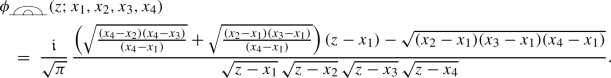

  

• For general N and $\beta \in \text {LP}_N$, one can derive an explicit expression for $\phi _\beta$ using Cramer’s rule.

3.3 Proof of Proposition 3.6 and emergence of $\mathcal {F}_\beta$

Our first goal is to show Proposition 3.6 via two auxiliary Lemmas 3.10 and A.1 (the latter in Appendix A). To this end, we first set some notation. For $2\le r \le N$, we define row vectors $\smash {\varvec{U}_{\beta }^{\pm }(r)}$ of size $N-1$ as

$$\begin{aligned} \varvec{U}_{\beta }^{\pm }(r) := \big ( U_{\beta }^{\pm }(r,1), \, U_{\beta }^{\pm }(r,2), \, \ldots , \, U_{\beta }^{\pm }(r,N-1) \big ) , \end{aligned}$$

where for $2\le r \le N$ and $0 \le s \le N-1$, we denote

$$\begin{aligned} U_{\beta }^{+}(r,s) := \;&(x_{a_{r}} - x_1)^s \, \ddot{S}^{a_{r}, b_{r}}_{x_1, \ldots , x_{2N}}(x_{a_{r}}) \nonumber \\ U_{\beta }^{-}(r,s) := \;&(x_{b_{r}}-x_1)^s \, \ddot{S}^{a_{r}, b_{r}}_{x_1, \ldots , x_{2N}}(x_{b_{r}}) , \end{aligned}$$

(3.10)

and where the function

$$\begin{aligned} z \;&\longmapsto \sqrt{z-x_{a_r}} \, \sqrt{z-x_{b_r}} \, S_{\varvec{x}}(z) =: \underset{j\notin \{a_{r}, b_{r}\}}{\prod } \frac{1}{\sqrt{z - x_j}} =: \ddot{S}^{a_{r}, b_{r}}_{x_1, \ldots , x_{2N}}(z) \end{aligned}$$

is holomorphic and single-valued on a Riemann surface $\Sigma _{\varvec{x}} = \Sigma _{x_1, \ldots , x_{2N}}$ as in Remark 3.8. We also define an $(N-1) \times (N-1)$-matrix

$$\begin{aligned} R_{\beta } := \begin{pmatrix} \varvec{U}_{\beta }^{+}(2) \, + \, \varvec{U}_{\beta }^{-}(2) \\ \cdot \\ \cdot \\ \cdot \\ \varvec{U}_{\beta }^{+}(N) \, + \, \varvec{U}_{\beta }^{-}(N) \end{pmatrix}, \end{aligned}$$

(3.11)

that is, we define $R_{\beta }(r,s):=U_{\beta }^{+}(r+1,s)+U_{\beta }^{-}(r+1,s)$ for $1\le r \le N-1$ and $1\le s\le N-1$. Note that writing $\varvec{\hat{\sigma }} = (\hat{\sigma }_2, \ldots , \hat{\sigma }_N)\in \{\pm 1\}^{N-1}$, and identifying $\pm 1$ with the superscript ±, we have

$$\begin{aligned} \det (R_{\beta }) = \sum _{\varvec{\hat{\sigma }} \in \{\pm 1\}^{N-1}}Q_{\beta } (\varvec{\hat{\sigma }}) , \quad \text {where} \quad Q_{\beta } (\varvec{\hat{\sigma }}) := \det \begin{pmatrix} \varvec{U}_{\beta }^{\hat{\sigma }_2}(2) \\ \cdot \\ \cdot \\ \cdot \\ \varvec{U}_{\beta }^{\hat{\sigma }_{N}}(N) \end{pmatrix}. \end{aligned}$$

(3.12)

Proof of Proposition 3.6

We write the polynomial $P_{\beta }$ as

$$\begin{aligned} P_{\beta }(z) = p_0 + p_1(z-x_1) + \cdots + p_{N-1}(z-x_1)^{N-1}, \end{aligned}$$

where $p_0, p_1, \ldots , p_{N-1} \in \mathbb {R}$ are some real coefficients. Note that $p_0=P_{\beta }(x_1)$ and $p_1=P_{\beta }'(x_1)$. Defining an $(N-1)$-component vector $\varvec{V}_{\beta } = \big ( V_{\beta }(1), \, V_{\beta }(2), \, \ldots , \, V_{\beta }(N-1) \big )$ with entries

$$\begin{aligned} V_{\beta }(r) := R_{\beta }(r,0) , \quad 1\le r \le N-1 , \end{aligned}$$

(3.13)

we note that the restrictions (3.5) and (3.6) read

$$\begin{aligned} \sqrt{\pi } \, \mathfrak {i}\, p_0 \, S_{x_2, x_3, \ldots , x_{2N}}(x_1)&= 1 , \end{aligned}$$

(3.14)

$$\begin{aligned} \sum _{n=1}^{N-1} \frac{p_n}{p_0} \, R_{\beta }(r,n)&= - V_{\beta }(r), \quad 1\le r \le N-1 , \end{aligned}$$

(3.15)

where $S_{x_2, x_3, \ldots , x_{2N}}(z) = \underset{j \ne 1}{\prod } \frac{1}{\sqrt{z - x_j}}:= \sqrt{z-x_{1}} \, S_{\varvec{x}}$ is holomorphic and single-valued on $\Sigma _{\varvec{x}}$ as in Remark 3.8. Proposition 3.6 now follows by showing that the matrix $R_{\beta }$ in (3.11) is invertible (Lemma 3.10). $\square$

Lemma 3.10

The matrix $R_{\beta }$ defined by (3.11) is invertible.

Proof

We need to show that $\det (R_{\beta })$ in (3.12) is non-zero. Write

$$\begin{aligned} y_r^{+, \beta } := x_{a_r} \quad \text {and} \quad y_r^{-, \beta } := x_{b_r} , \quad 2\le r \le N . \end{aligned}$$

(3.16)

Using the Vandermonde determinant, we have

$$\begin{aligned} Q_{\beta } (\varvec{\hat{\sigma }}) =&\; Q_{\beta }(\hat{\sigma }_2, \ldots , \hat{\sigma }_N) \nonumber \\ =&\; \prod _{2\le r \le N} \big ( y_r^{\hat{\sigma }_r, \beta } - x_1 \big ) \; \prod _{2\le s < t\le N} \big ( y_t^{\hat{\sigma }_t, \beta } - y_s^{\hat{\sigma }_s, \beta } \big ) \; \prod _{2\le r \le N} \ddot{S}^{a_{r}, b_{r}}_{x_1, \ldots , x_{2N}} \big ( y_r^{\hat{\sigma }_r, \beta } \big ) . \end{aligned}$$

(3.17)

From Lemma A.1, we find a constant $\theta _{\beta }\in \{ \pm 1, \pm \mathfrak {i}\}$ depending only on $\beta$ such that

$$\begin{aligned} \frac{Q_{\beta }(\varvec{\hat{\sigma }})}{\theta _{\beta }} > 0 . \end{aligned}$$

(3.18)

Combining (3.12) with (3.18), we obtain $\frac{\det R_{\beta }}{\theta _{\beta }} > 0$, which implies that $R_{\beta }$ is invertible. $\square$

The second goal of this section is to derive the expansion of $\phi _{\beta }$ as $z\rightarrow x_1$ (Lemma 3.11) and to relate its expansion coefficients to the partition function $\mathcal {F}_{\beta }$ defined in (1.16) (Proposition 3.12).

Lemma 3.11

Write $\varvec{x}=(x_1, \ldots , x_{2N})\in \mathfrak {X}_{2N}$. The holomorphic function (3.4) on $\Sigma _{\varvec{x}}$ satisfies

$$\begin{aligned} \phi _{\beta }(z; \varvec{x}) = \frac{1}{\sqrt{\pi } \, \sqrt{z-x_1}} + \mathcal {K}_{\beta }(\varvec{x}) \, \sqrt{z-x_1} + o(\sqrt{z-x_1}) , \quad \text {as} \quad z\rightarrow x_1 , \end{aligned}$$

where

$$\begin{aligned} \mathcal {K}_{\beta }(\varvec{x}) = \mathcal {K}_{\beta }(x_1, \ldots , x_{2N}) = \frac{1}{\sqrt{\pi }} \bigg ( \frac{P_{\beta }'(x_1)}{P_{\beta }(x_1)}+\frac{1}{2}\sum _{k=2}^{2N}\frac{1}{x_k-x_1} \bigg ). \end{aligned}$$

(3.19)

Proof

From the expression in (3.4), we may write

$$\begin{aligned} \phi _{\beta }(z; \varvec{x}) = \frac{\mathcal {J}_{\beta }(\varvec{x})}{\sqrt{z-x_1}} + \mathcal {K}_{\beta }(\varvec{x}) \, \sqrt{z-x_1} + o(\sqrt{z-x_1}) , \quad \text {as}\quad z\rightarrow x_1 , \end{aligned}$$

where

$$\begin{aligned} \mathcal {J}_{\beta }(x_1, \ldots , x_{2N}) =&\; \mathfrak {i}\, P_{\beta }(x_1) \, S_{x_2, x_3, \ldots , x_{2N}}(x_1) , \\ \mathcal {K}_{\beta }(x_1, \ldots , x_{2N}) =&\; \mathfrak {i}\, P_{\beta }(x_1) \, S_{x_2, x_3, \ldots , x_{2N}}(x_1) \times \bigg ( \frac{P_{\beta }'(x_1)}{P_{\beta }(x_1)}+\frac{1}{2}\sum _{k=2}^{2N}\frac{1}{x_k-x_1} \bigg ) . \end{aligned}$$

From (3.14) with $p_0=P_{\beta }(x_1)$, we see that $\mathcal {J}_{\beta }=1/\sqrt{\pi }$ and (3.19) holds. This completes the proof. $\square$

Proposition 3.12

Write $\varvec{x}=(x_1, \ldots , x_{2N})\in \mathfrak {X}_{2N}$. We have

$$\begin{aligned} \partial _1\log \mathcal {F}_{\beta }(\varvec{x}) = \frac{\sqrt{\pi }}{4} \, \mathcal {K}_{\beta }(\varvec{x}), \end{aligned}$$

(3.20)

where $\mathcal {F}_{\beta }$ is defined in (1.16) and $\mathcal {K}_{\beta }$ is defined in (3.19).

Proof

On the one hand, let us compute $\partial _1\log \mathcal {F}_{\beta }(\varvec{x})$. For the cross-ratios, (recalling (3.1)) we have

$$\begin{aligned} \partial _1 \chi (x_1,x_{a_r},x_{b_r},x_{2\ell }) = -\chi (x_1,x_{a_r},x_{b_r},x_{2\ell }) \; \frac{x_{b_r}-x_{a_r}}{(x_{a_r}-x_1)(x_{b_r}-x_1)} , \quad 2\le r \le N . \end{aligned}$$

Thus, writing $\varvec{\sigma }=(\sigma _1, \ldots , \sigma _N)\in \{\pm 1\}^N$ and $\varvec{\hat{\sigma }}=(\hat{\sigma }_2, \ldots , \hat{\sigma }_N)\in \{\pm 1\}^{N-1}$, where the variables $\hat{\sigma }_r$ in $\varvec{\hat{\sigma }}$ could be viewed as products $\sigma _1\sigma _r$ of the variables $\sigma _1$ and $\sigma _r$ in $\varvec{\sigma }$ for $2\le r\le N$, and using the shorthand notation (1.17), we obtain

$$\begin{aligned}&8 \, \partial _1 \log \mathcal {F}_{\beta }(\varvec{x}) \, - \, \frac{1}{x_{2\ell }-x_1} \nonumber \\&\quad = \; \frac{ \sum _{\varvec{\sigma }\in \{\pm 1\}^{N}} {\Big (-\sigma _1 \sum _{r=2}^{N} \, \sigma _r \frac{x_{b_r}-x_{a_r}}{(x_{a_r}-x_1)(x_{b_r}-x_1)}\Big ) } \Big (\prod _{s=2}^{N} \, \chi _{1,a_s,b_s,2\ell }^{\sigma _1\sigma _s/4}\Big ) \Big (\prod _{2\le r< s \le N} \, \chi _{a_r,a_s,b_s,b_r}^{\sigma _r \sigma _s/4}\Big )}{ \sum _{\varvec{\sigma }\in \{\pm 1\}^{N}} \Big ( \prod _{s=2}^{{N}} \, \chi _{1,a_s,b_s,2\ell }^{\sigma _1\sigma _s/4}\Big ) \Big ( \prod _{2\le r< s \le N} \, \chi _{a_r,a_s,b_s,b_r}^{\sigma _r \sigma _s/4}\Big )} \nonumber \\&\quad = \; \frac{ \sum _{\varvec{\hat{\sigma }}\in \{\pm 1\}^{N-1}} { \Big (-\sum _{r=2}^{{N}} \, \hat{\sigma }_r \frac{x_{b_r}-x_{a_r}}{(x_{a_r}-x_1)(x_{b_r}-x_1)}\Big ) } \Big (\prod _{s=2}^{{N}} \, \chi _{1,a_s,b_s,2\ell }^{\hat{\sigma }_s/4}\Big ) \Big (\prod _{2\le r< s \le N} \, \chi _{a_r,a_s,b_s,b_r}^{\hat{\sigma }_r \hat{\sigma }_s/4}\Big )}{ \sum _{\varvec{\hat{\sigma }}\in \{\pm 1\}^{N-1}} \Big ( \prod _{s=2}^{{N}} \, \chi _{1,a_s,b_s,2\ell }^{\hat{\sigma }_s/4}\Big ) \Big (\prod _{2\le r< s \le N} \, \chi _{a_r,a_s,b_s,b_r}^{\hat{\sigma }_r \hat{\sigma }_s/4}\Big )} \nonumber \\&\quad = \; \frac{ \sum _{\varvec{\hat{\sigma }}\in \{\pm 1\}^{N-1}} { \Big (-\sum _{r=2}^{{N}} \, \hat{\sigma }_r\frac{x_{b_r}-x_{a_r}}{(x_{a_r}-x_1)(x_{b_r}-x_1)}\Big ) } \Big (\prod _{s=2}^{{N}} \, \chi _{1,a_s,b_s,2\ell }^{(\hat{\sigma }_s+1)/4}\Big ) \Big (\prod _{2\le r< s \le N} \, \chi _{a_r,a_s,b_s,b_r}^{(\hat{\sigma }_r \hat{\sigma }_s + 1)/4}\Big )}{\sum _{\varvec{\hat{\sigma }}\in \{\pm 1\}^{N-1}} \Big ( \prod _{s=2}^{{N}} \, \chi _{1,a_s,b_s,2\ell }^{(\hat{\sigma }_s+1)/4}\Big ) \Big (\prod {2\le r< s \le N} \, \chi _{a_r,a_s,b_s,b_r}^{(\hat{\sigma }_r \hat{\sigma }_s + 1)/4}\Big )}, \end{aligned}$$

(3.21)

On the other hand, let us compute $\mathcal {K}_{\beta }(\varvec{x})$. We denote by $R^{\bullet }_{\beta }$ the $(N-1)\times (N-1)$-matrix obtained by replacing the first column of $R_{\beta }$ by the column vector $\smash {\varvec{V}_{\beta } = \big ( V_{\beta }(1), \, V_{\beta }(2), \, \ldots , \, V_{\beta }(N-1) \big )^t}$ defined in (3.13). Then, combining (3.15) with Cramer’s rule, we find that

$$\begin{aligned} \frac{P_{\beta }'(x_1)}{P_{\beta }(x_1)}=-\frac{\det (R_{\beta }^{\bullet })}{\det (R_{\beta })}. \end{aligned}$$

(3.22)

Using Lemma A.2 (from Appendix A) we can find functions $g^{\varvec{\hat{\sigma }}, \beta }(\varvec{x})>0$ for $\varvec{\hat{\sigma }}=(\hat{\sigma }_2,\ldots ,\hat{\sigma }_{N})\in \{\pm 1\}^{N-1}$ such that

$$\begin{aligned} \frac{\det (R_{\beta }^{\bullet })}{\det (R_{\beta })} = \frac{\sum _{\varvec{\hat{\sigma }}\in \{\pm 1\}^{N-1}} \, g^{\varvec{\hat{\sigma }}, \beta }(\varvec{x}) \; \sum _{r=2}^{{N}} \; \big ( y_{r}^{\hat{\sigma }_r, \beta } - x_1 \big )^{-1} }{\sum _{\varvec{\hat{\sigma }}\in \{\pm 1\}^{N-1}} \; g^{\varvec{\hat{\sigma }}, \beta }(\varvec{x})} , \end{aligned}$$

(3.23)

where $y_{r}^{\hat{\sigma }_r, \beta }$ are defined in (3.16). Lemma A.3 (from Appendix A) implies that there exist functions $f_{\beta }(\varvec{x})>0$ such that, for all $\varvec{\hat{\sigma }}=(\hat{\sigma }_2, \ldots , \hat{\sigma }_N)\in \{\pm 1\}^{N-1}$, we have

$$\begin{aligned} g^{\varvec{\hat{\sigma }}, \beta }(\varvec{x}) = f_{\beta }(\varvec{x}) \; \prod _{2\le r \le N}\chi _{1,a_r,b_r,2\ell }^{\frac{\hat{\sigma }_r+1}{4}} \prod _{2\le s < t \le N}\chi _{a_s,a_t,b_t,b_s}^{\frac{\hat{\sigma }_s \hat{\sigma }_t+1}{4}} . \end{aligned}$$

(3.24)

Plugging all of (3.22, 3.23, 3.24) into (3.19), and recalling (3.1), we obtain

$$\begin{aligned} 2\sqrt{\pi } \, \mathcal {K}_{\beta }(\varvec{x}) = \;&2\frac{P_{\beta }'(\varvec{x})}{P_{\beta }(\varvec{x})} \, + \, \sum _{k=2}^{2N} \frac{1}{x_{k}-x_1} \\ = \;&\frac{1}{x_{2\ell }-x_1} \, + \, 2\frac{P_{\beta }'(\varvec{x})}{P_{\beta }(\varvec{x})} \, + \, \sum _{k=2}^{N} \Big ( \frac{1}{x_{a_k}-x_1}+\frac{1}{x_{b_k}-x_1} \Big )\\ = \;&\frac{1}{x_{2\ell }-x_1} \, + \, {(3.21)}, \end{aligned}$$

where we also used the identity

$$\begin{aligned} -2\sum _{r=2}^N \frac{1}{y_r^{\hat{\sigma }_r,\beta }-x_1}+\sum _{r=2}^N \left( \frac{1}{x_{a_r}-x_1}+\frac{1}{x_{b_r}-x_1}\right) =\sum _{r=2}^N \hat{\sigma }_r\left( \frac{1}{x_{b_r}-x_1}-\frac{1}{x_{a_r}-x_1}\right) \end{aligned}$$

for all $\varvec{\hat{\sigma }}=(\hat{\sigma }_2,\ldots ,\hat{\sigma }_{N})\in \{\pm 1\}^{N-1}$. This gives the asserted identity (3.20). $\square$

We fill in the details to finish the proof of Proposition 3.12 (Lemmas A.2 and A.3) in Appendix A.

3.4 Scaling limit of the observable: proof of Proposition 3.5

Some key ideas in the proof of Proposition 3.5 are learned from [16, 41]—we adjust them to deal with the FK-Ising model in polygons in our setup. We first fix some terminology on discrete complex analysis—see [15] for more details on discrete harmonicity, holomorphicity, and s-holomorphicity.

• We say that a function $u :\mathbb {Z}^2 \rightarrow \mathbb {C}$ is (discrete) harmonic (resp. sub/superharmonic) at a vertex $z \in \mathbb {Z}^2$ if $\Delta u(z):= \sum _{w \sim z} (u(w)-u(z))=0$ (resp. $\Delta u(z) \ge 0$, $\Delta u(z) \le 0$), where the sum is taken over all neighbors of z. We say that a function u is harmonic (resp. sub/superharmonic) on a subgraph of $\mathbb {Z}^2$ if u is harmonic (resp. sub/superharmonic) at all vertices of this subgraph.

• We say that a function $\phi :\mathbb {Z}^2 \cup (\mathbb {Z}^2)^{\bullet }\rightarrow \mathbb {C}$ is (discrete) holomorphic around a medial vertex $z^\diamond$ if the (discrete) Cauchy–Riemann equation at $z^\diamond$ holds: $\phi (n)-\phi (s)=\mathfrak {i}(\phi (e)-\phi (w))$, where n, w, s, e are the vertices incident to $z^\diamond$ in counterclockwise order (two of them are primal vertices while the other two are dual vertices).

• We say that a function $f :(\mathbb {Z}^2)^\diamond \rightarrow \mathbb {C}$ is spin-holomorphic (s-holomorphic) around a medial edge $e^\diamond$ if

  $$\begin{aligned} \text {Proj}_{\nu (e^\diamond ) \, \mathbb {R}}[f(z_-^\diamond )] = \text {Proj}_{\nu (e^\diamond ) \, \mathbb {R}}[f(z_+^\diamond )] , \end{aligned}$$

  where $z_-^\diamond$ and $z_+^\diamond$ are endpoints of the medial edge $e^\diamond$, and $\text {Proj}_{L}$ is the orthogonal projection onto the line L on the complex plane. Note that, if f is s-holomorphic around all medial edges of $\Omega ^{\delta ,\diamond }$ that are not adjacent to the marked medial vertices, then it is holomorphic around all interior vertices of $\Omega ^{\delta }$ and around all interior dual vertices of $\Omega ^{\delta ,\bullet }$ (see, e.g., [69, Remark 3.3]).

The next lemma shows that the observable $F_{\beta }^{\delta }$ has Riemann type boundary behavior.

Lemma 3.13

The observable $F_{\beta }^{\delta }$ has the following properties.

• 1 . If $e^{\diamond }$ is a medial edge connecting two vertices on $\partial \Omega ^{\delta ,\diamond }{\setminus } \{x_1^{\delta ,\diamond },x_2^{\delta ,\diamond },\ldots ,x_{2N}^{\delta ,\diamond }\}$, then $F_{\beta }^{\delta }(e^{\diamond })\parallel \nu (e^{\diamond })$.

• 2 . If $x^{\diamond } \in \partial \Omega ^{\delta ,\diamond }$ is a medial vertex lying on some primal edge in $\smash {\bigcup _{r=1}^{N}} (x_{2r-1}^{\delta } \, x_{2r}^{\delta })$, then $F_{\beta }^{\delta }(x^{\diamond })\parallel \frac{1}{\sqrt{e(x^{\diamond })}}$, where $e(x^{\diamond })$ is the primal edge having $x^{\diamond }$ as its midpoint, oriented to have the primal polygon on its left, and the branch choice of the square root is arbitrary.

• 3 . If $x^{\diamond } \in \partial \Omega ^{\delta ,\diamond }$ is a medial vertex lying on some dual edge in $\smash {\bigcup _{r=1}^{N}} (x_{2r}^{\delta ,\bullet } \, x_{2r+1}^{\delta ,\bullet })$, then $F_{\beta }^{\delta }(x^{\diamond }) \parallel \frac{\mathfrak {i}}{\sqrt{e(x^{\diamond })}}$, where $e(x^{\diamond })$ is the dual edge having $x^{\diamond }$ as its midpoint, oriented to have the dual polygon on its left, and the branch choice of the square root is arbitrary.

Proof

The same argument as in [69, Lemma 4.1] proves Item 1. Covering both Items 2 and 3, suppose that $x^{\diamond } \in (x_{i}^{\delta ,\diamond } \, x_{i+1}^{\delta ,\diamond })$. Let $e_-^{\diamond }, e_+^{\diamond } \in (x_{i}^{\delta ,\diamond } \, x_{i+1}^{\delta ,\diamond })$ be the oriented medial edges having $x^{\diamond }$ as end vertex and beginning vertex, respectively. It follows from Definition 3.3 (recalling also (3.1)) of the exploration path $\xi ^{\delta }$ that it passes through $e_-^{\diamond }$ if and only if it passes through $e_+^{\diamond }$. Moreover, when $\xi ^{\delta }$ passes through $e_-^{\diamond }$, the winding is

$$\begin{aligned} W_{\xi ^{\delta }} \big ( e_{2\ell }^{\delta ,\diamond },e_+^{\diamond } \big ) = {\left\{ \begin{array}{ll} W_{\xi ^{\delta }} \big ( e_{2\ell }^{\delta ,\diamond },e_-^{\diamond } \big ) + \frac{\pi }{2} , &{} \text {if}\quad i \text { is odd;}\\ W_{\xi ^{\delta }} \big ( e_{2\ell }^{\delta ,\diamond },e_-^{\diamond } \big ) - \frac{\pi }{2} , &{} \text {if}\quad i \text { is even.} \end{array}\right. } \end{aligned}$$

Consequently, we have

$$\begin{aligned} F_{\beta }^{\delta }(e_+^{\diamond }) = {\left\{ \begin{array}{ll} F_{\beta }^{\delta }(e_-^{\diamond })\exp (-\mathfrak {i}\frac{\pi }{4}), &{} \text {if}\quad i \text { is odd},\\ F_{\beta }^{\delta }(e_-^{\diamond })\exp (\mathfrak {i}\frac{\pi }{4}), &{} \text {if}\quad i \text { is even}. \end{array}\right. } \end{aligned}$$

(3.25)

Thus, by (3.2) and (3.25), we have

$$\begin{aligned} {\left\{ \begin{array}{ll} F_{\beta }^{\delta }(x^{\diamond }) \parallel F_{\beta }^{\delta }(e_-^{\diamond })\exp (-\mathfrak {i}\frac{\pi }{8}), &{} \text {if}\quad i \text { is odd},\\ F_{\beta }^{\delta }(x^{\diamond }) \parallel F_{\beta }^{\delta }(e_-^{\diamond })\exp (\mathfrak {i}\frac{\pi }{8}), &{}\text {if}\quad i \text { is even}. \end{array}\right. } \end{aligned}$$

(3.26)

Items 2 and 3 now follow from (3.26) and Item 1. $\square$

The key property of the observable $F_{\beta }^{\delta }$ is its discrete holomorphicity.

Lemma 3.14

If $z^{\diamond }$ and $w^{\diamond }$ are either two interior vertices of $\Omega ^{\delta ,\diamond }$, or two boundary vertices such that $z^{\diamond }, w^{\diamond } \in \smash {\bigcup _{r=1}^{N}} (x_{2r}^{\delta ,\diamond } \, x_{2r+1}^{\delta ,\diamond }){\setminus }\{x_1^{\delta ,\diamond },x_2^{\delta ,\diamond },\ldots ,x_{2N}^{\delta ,\diamond }\}$, and $e^{\diamond }$ is the medial edge connecting them, then $F_{\beta }^{\delta }$ is s-holomorphic around $e^{\diamond }$, that is,

$$\begin{aligned} \text {Proj}_{\nu (e^{\diamond }) \, \mathbb {R}}\left[ F_{\beta }^{\delta }(z^{\diamond })\right] =\text {Proj}_{\nu (e^{\diamond }) \, \mathbb {R}}\left[ F_{\beta }^{\delta }(w^{\diamond })\right] =F_{\beta }^{\delta }(e^{\diamond }). \end{aligned}$$

(3.27)

In particular, the vertex observable $F_{\beta }^{\delta }$ is holomorphic around all interior vertices of $\Omega ^{\delta }$ and around all interior dual vertices of $\Omega ^{\delta ,\bullet }$.

Proof

If $z^{\diamond }, w^{\diamond } \in \smash {\bigcup _{r=1}^{N}} (x_{2r}^{\delta ,\diamond } \, x_{2r+1}^{\delta ,\diamond }){\setminus }\{x_1^{\delta ,\diamond },x_2^{\delta ,\diamond },\ldots ,x_{2N}^{\delta ,\diamond }\}$, then (3.27) follows immediately from the definition (3.2) of $F_{\beta }^{\delta }$ together with Item 1 of Lemma 3.13 and the observation (3.25). For two interior medial vertices (3.27) follows from [69, Lemma 4.5]. The discrete holomorphicity of the vertex observable $F_{\beta }^{\delta }$ can be deduced from its s-holomorphicity (see, e.g., [69, Remark 3.3]). $\square$

From Lemma 3.14 and [69, Lemma 3.6], we see that there exists a unique function (the imaginary part of the discrete “primitive” of $(F_{\beta }^{\delta })^2$)

$$\begin{aligned} H^{\delta }_{\beta } :\Omega ^\delta \cup \Omega ^{\delta ,\bullet }\rightarrow \mathbb {R}\quad \text {such that} \quad {\left\{ \begin{array}{ll} H^{\delta }_{\beta }(x_{1}^{\delta }) = 0 , \\ H^{\delta }_{\beta }(w^{\bullet }) - H^{\delta }_{\beta }(z) = \big | \text {Proj}_{\nu (e^{\diamond }) \, \mathbb {R}} [F_{\beta }^{\delta }(e^{\diamond }) ] \big |^2 , \end{array}\right. } \end{aligned}$$

for each medial edge $e^{\diamond }$ bordered by a primal vertex $z \in \Omega ^\delta$ and a dual vertex $w^{\bullet } \in \Omega ^{\delta ,\bullet }$. Let $\smash {H^{\delta ,\bullet }_{\beta }}$ and $\smash {H^{\delta ,\circ }_{\beta }}$ be the restrictions of $H_{\beta }^{\delta }$ on $\Omega ^{\delta ,\bullet }$ and $\Omega ^{\delta }$, respectively. Note that, if $z,w \in \Omega ^{\delta }$ are two neighboring primal vertices, then we have (see, e.g., [69, Remark 3.7])

$$\begin{aligned} H^{\delta ,\circ }_{\beta }(z) - H^{\delta ,\circ }_{\beta }(w) = {\text {Im}}\bigg ( \frac{\big (F_{\beta }^{\delta }(\frac{z+w}{2})\big )^2}{\sqrt{2}\delta } (z - w) \bigg ) . \end{aligned}$$

(3.28)

Notably, the function $H^{\delta }_{\beta }$ has Dirichlet type boundary conditions that are more directly related to the exploration path—see Eq. (3.29) in the next lemma.

Lemma 3.15

There exist constants $(C_1^{\delta },\ldots ,C_{2N}^{\delta }) \in \mathbb {R}^{2N}$ with $C_{1}^{\delta }=0$ such that the following hold.

• 1 . The function $\smash {H^{\delta ,\bullet }_{\beta }}$ is subharmonic on the interior vertices of $\Omega ^{\delta ,\bullet }$. The function $\smash {H^{\delta ,\circ }_{\beta }}$ is superharmonic on the interior vertices of $\Omega ^{\delta }$. For each $r \in \{1,2,\ldots ,N\}$, we have the boundary values

  $$\begin{aligned} {\left\{ \begin{array}{ll} H^{\delta ,\bullet }_{\beta } = C_{2r}^{\delta } &{} \text {on} \quad \left( x_{2r}^{\delta ,\bullet } \, x_{2r+1}^{\delta ,\bullet }\right) , \\ H^{\delta ,\circ }_{\beta } = C_{2r-1}^{\delta } &{} \text {on} \quad \left( x_{2r-1}^{\delta } \, x_{2r}^{\delta }\right) . \end{array}\right. } \end{aligned}$$

• 2 . For each $r \in \{1,2,\ldots ,N\}$, set $H^{\delta ,\bullet }_{\beta }:= C_{2r-1}^{\delta }$ on dual vertices in $(\delta \mathbb {Z}^2)^{\bullet } {\setminus } \Omega ^{\delta ,\bullet }$ adjacent to $(x_{2r-1}^{\delta ,\bullet } \, x_{2r}^{\delta ,\bullet })$ and $H^{\delta ,\circ }_{\beta }:= C_{2r}^{\delta }$ on primal vertices in $\delta \mathbb {Z}^2 {\setminus } \Omega ^{\delta }$ adjacent to $(x_{2r}^{\delta } \, x_{2r+1}^{\delta })$. Then, the function $\smash {H^{\delta ,\bullet }_{\beta }}$ is also subharmonic at all $z^{\bullet } \in \smash {\bigcup _{r=1}^{N}} (x_{2r-1}^{\delta ,\bullet } \, x_{2r}^{\delta ,\bullet })$ with Laplacian modified on the boundary:

  $$\begin{aligned} \Delta H^{\delta ,\bullet }_{\beta }(z^{\bullet }) := \sum _{w^{\bullet }\sim z^{\bullet }} d(z^{\bullet },w^{\bullet }) \, \left( H^{\delta ,\bullet }_{\beta }(w^{\bullet })-H^{\delta ,\bullet }_{\beta }(z^{\bullet })\right) \ge 0 , \end{aligned}$$

  where $d(z^{\bullet },w^{\bullet }):=1$ if $w^{\bullet } \in \Omega ^{\delta ,\bullet }$ and $d(z^{\bullet },w^{\bullet }):=2\tan \frac{\pi }{8}=2(\sqrt{2}-1)$ if $w^{\bullet }\notin \Omega ^{\delta ,\bullet }$.

  Besides, $\smash {H^{\delta ,\circ }_{\beta }}$ is superharmonic at all $z \in \smash {\bigcup _{r=1}^{N}} (x_{2r}^{\delta } \, x_{2r+1}^{\delta })$ with Laplacian modified on the boundary:

  $$\begin{aligned} \Delta H^{\delta ,\circ }_{\beta }(z) := \sum _{w \sim z} d(z,w) \, \left( H^{\delta ,\circ }_{\beta }(w) - H^{\delta ,\circ }_{\beta }(z)\right) \le 0 , \end{aligned}$$

  where $d(z,w):= 1$ if $w \in \Omega ^{\delta }$ and $d(z,w) = 2(\sqrt{2}-1)$ if $w \notin \Omega ^{\delta }$.

• 3 . For each $r \in \{1,2,\ldots ,N\}$, we have $C_{2r}^{\delta }\ge C_{2r-1}^{\delta }$ and $C_{2r}^{\delta }\ge C_{2r+1}^{\delta }$.

• 4 . For each $r \in \{1,2,\ldots ,N\}$, we have

  $$\begin{aligned} |C_{a_r-1}^{\delta }-C_{a_r}^{\delta }|&= |C_{b_r-1}^{\delta }-C_{b_r}^{\delta }| \nonumber \\&= \left( \mathbb {P}_{\beta }^{\delta } \left[ \xi ^{\delta } \text { passes through the outer corners } y_{a_r}^{\delta ,\diamond } \text { and } y_{b_r}^{\delta ,\diamond } \right] \right) ^2. \end{aligned}$$

  (3.29)

  In particular, we have $|C_{1}^{\delta }-C_{2N}^{\delta }|=1$. As a consequence, the family $\{ C_1^{\delta },\ldots ,C_{2N}^{\delta } \}_{\delta >0}$ of constants is uniformly bounded.

Proof

The subharmonicity of $\smash {H^{\delta ,\bullet }_{\beta }}$ and superharmonicity of $\smash {H^{\delta ,\circ }_{\beta }}$ on interior vertices both follow from [69, Lemma 3.8]. By construction, $\smash {H^{\delta ,\bullet }_{\beta }}$ is constant on $(x_{2r}^{\delta ,\bullet } \, x_{2r+1}^{\delta ,\bullet })$ and $\smash {H^{\delta ,\circ }_{\beta }}$ is constant on $(x_{2r-1}^{\delta } \, x_{2r}^{\delta })$. This gives Item 1. Item 2 follows from [16, Lemma 3.14]. Item 3 and relation (3.29) hold by construction. The identity $|C_{1}^{\delta }-C_{2N}^{\delta }|=1$ follows from (3.29) since $\xi ^{\delta }$ goes through $y_{1}^{\delta ,\diamond }$ with probability one. Lastly, as $C_{1}^{\delta }=0$, we find from (3.29) that $|C_{k}^{\delta }|\le 2N-1$, for all $\delta >0$ and $1 \le k \le 2N$. $\square$

We see from Lemma 3.15 that the collection $\{ C_1^{\delta },\ldots ,C_{2N}^{\delta } \}_{\delta >0}$ of constants has convergent subsequences. For the convergence of the observable, we also need the following key lemma.

Lemma 3.16

Assume the same setup as in Proposition 3.5. We extend $H^{\delta }_{\beta }$ to continuous functions on the planar domains corresponding to $\Omega ^{\delta ,\diamond }$ via linear interpolation. Then, the sequence

$$\begin{aligned} \left\{ \left( 2^{-1/4}\delta ^{-1/2} \, F^{\delta }_{\beta }, \, H^{\delta }_{\beta }\right) \right\} _{\delta >0} \end{aligned}$$

has (locally uniformly) convergent subsequences. Moreover, any subsequential limit $(F_{\beta },H_{\beta })$, with also $(C_1^\delta ,C_2^\delta ,\ldots ,C_{2N}^\delta )$ converging to some $(C_1,C_2,\ldots ,C_{2N})\in \mathbb {R}^{2N}$, satisfies the following properties.

• 1 . The function $F_{\beta }$ is holomorphic on $\Omega$, and $H_{\beta }(w)={\text {Im}}\int ^w F_{\beta }(z)^2 \, \text {d}z$ on $\Omega \ni w$.

• 2 . The function $H_{\beta }$ is bounded and harmonic on $\Omega$.

• 3 . We have $H_{\beta }(z)\rightarrow C_k$ as $z\rightarrow (x_k \, x_{k+1})$ in $\mathbb {H}$, for all $k \in \{1,2,\ldots ,2N\}$.

• 4 . The relations $C_{2r} \ge C_{2r-1}$ and $C_{2r} \ge C_{2r+1}$ hold for all $r \in \{1,2,\ldots ,N\}$.

• 5 . The relation $|C_{a_r-1}-C_{a_r}| = |C_{b_r-1}-C_{b_r}|$ holds for all $r \in \{1,2,\ldots ,N\}$, and we have $|C_{1}-C_{2N}|=1$.

• 6 . The outer normal derivative $\partial _{\text {n}} H_{\beta }$ of the function $H_{\beta }$ satisfies $\partial _{\text {n}} H_{\beta }\ge 0$ on $\smash {\bigcup _{r=1}^{N}} (x_{2r} \, x_{2r+1})$ and $\partial _{\text {n}} H_{\beta }\le 0$ on $\smash {\bigcup _{r=1}^{N}} (x_{2r-1} \, x_{2r})$ in the following sense: if $z\in (x_{2r} \, x_{2r+1})$ for some r, then

  $$\begin{aligned} H_{\beta }^{-1}( {-\infty } , C_{2r}] \cap \{w \in \Omega :|w-z|<\epsilon \} \ne \emptyset , \quad \text {for all} \quad \epsilon > 0, \end{aligned}$$

  while if $z\in (x_{2r-1} \, x_{2r})$ for some r, then

  $$\begin{aligned} H_{\beta }^{-1} [C_{2r-1},\infty ) \cap \{w \in \Omega :|w-z|<\epsilon \} \ne \emptyset , \quad \text {for all} \quad \epsilon > 0 . \end{aligned}$$

Proof

The sequence $\{H_{\beta }^{\delta }\}_{\delta >0}$ is uniformly bounded by Items 1 and 4 of Lemma 3.15: we have

$$\begin{aligned} |H_{\beta }^{\delta }| \le M , \quad \text {for all}\quad \delta > 0 , \end{aligned}$$

(3.30)

with some $M\in (0,\infty )$. Thus, the sequence $\big \{ (2^{-1/4}\delta ^{-1/2} \, F^{\delta }_{\beta }, \, H^{\delta }_{\beta }) \big \}_{\delta >0}$ has (locally uniformly) convergent subsequences by [16, Theorem 3.12]. Item 4 of Lemma 3.15 ensures that $\{(C_{1}^{\delta },C_{2}^{\delta },\ldots ,C_{2N}^{\delta })\}_{\delta >0}$ has convergent subsequences. Let $(F_{\beta },H_{\beta })$ be any subsequential limit along a sequence $\delta _n \rightarrow 0$ as $n \rightarrow \infty$ of $\big \{ (2^{-1/4}\delta ^{-1/2} \, F^{\delta }_{\beta }, \, H^{\delta }_{\beta }) \big \}_{\delta >0}$ with $(C_{1}^{\delta _n},\ldots ,C_{2N}^{\delta _n})$ also converging to some $(C_{1},\ldots ,C_{2N})\in \mathbb {R}^{2N}$ (choosing a simultaneously convergent subsequence by refining the sequence if necessary). Since $F_{\beta }^{\delta }$ is (discrete) holomorphic for each $\delta >0$ (Lemma 3.14) and the convergence is locally uniform, the limit $F_{\beta }$ is holomorphic due to Morera’s theorem. By (3.28) and the locally uniform convergence, we obtain the relation $H_{\beta }(w)={\text {Im}}\int ^w F_{\beta }(z)^2 \, \text {d}z$. Being the imaginary part of the holomorphic function $w \mapsto \int ^{w} F_{\beta }(z)^2 \, \text {d}z$, the function $H_{\beta }(w)$ is harmonic on $\Omega$, and (3.30) implies that $H_{\beta }$ is bounded on $\Omega$. This proves Items 1 and 2.

Next, fix $r \in \{1,2,\ldots ,N\}$. We will prove that $H_{\beta }(z)\rightarrow C_{2r-1}$ as $z\rightarrow (x_{2r-1} \, x_{2r})$. Let $z \in \Omega$ be any point. On the one hand, let $\{z^{\delta _n}\}_{n \ge 1}$ be a sequence of interior primal vertices approximating z. Denote by $\text {Hm}(z^{\delta _n}; E; \Omega ^{\delta _n})$ the discrete harmonic measure of $E \subset \partial \Omega ^{\delta _n}$ viewed from $z^{\delta _n}$. Then, we have

$$\begin{aligned} H_{\beta }(z) = \;&\lim _{n \rightarrow \infty } H_{\beta }^{\delta _n,\circ }(z^{\delta _n}) \\ \ge \;&\limsup _{n \rightarrow \infty } \left( C_{2r-1}^{\delta _n} \, \text {Hm}\left( z^{\delta _n};(x_{2r-1}^{\delta _n} \, x_{2r}^{\delta _n});\Omega ^{\delta _n}\right) - M \, \text {Hm}\left( z^{\delta _n};(x_{2r}^{\delta _n} \, x_{2r-1}^{\delta _n});\Omega ^{\delta _n}\right) \right) \\ = \;&C_{2r-1} \, \text {Hm}\left( z;(x_{2r-1} \, x_{2r});\Omega \right) - M \, \text {Hm}\left( z;(x_{2r} \, x_{2r-1});\Omega \right) , \end{aligned}$$

where the inequality in the second line follows from the superharmonicity of $\smash {H_{\beta }^{\delta _n,\circ }}$ (Items 1 and 2 of Lemma 3.15) and the fact that $\smash {H_{\beta }^{\delta _n,\circ }}$ takes the constant value $C_{2r-1}^{\delta _n}$ along $(x_{2r-1}^{\delta _n} \, x_{2r}^{\delta _n})$ (Item 1 of Lemma 3.15); and the equality in the third line is due to the convergence of the discrete polygons in the Carathéodory sense and [15, Theorem 3.12]. Therefore, we have

$$\begin{aligned} H_{\beta }(z) \ge C_{2r-1} - 2 M \, \text {Hm}\big (z;(x_{2r} \, x_{2r-1});\Omega \big ) . \end{aligned}$$

(3.31)

On the other hand, let $\{z^{\delta _n,\bullet }\}_{n \ge 1}$ be a sequence of interior dual vertices approximating z. Denote by $\text {Hm}(z^{\delta _n,\bullet };E;\Omega ^{\delta _n,\bullet })$ the discrete harmonic measure of $E \subset \partial \Omega ^{\delta _n,\bullet }$ viewed from $z^{\delta _n,\bullet }$. Then, we have

$$\begin{aligned} H_{\beta }(z)&= \lim _{n \rightarrow \infty } H_{\beta }^{\delta _n,\bullet }(z^{\delta _n,\bullet })\\&\le \liminf _{n \rightarrow \infty } \left( C_{2r-1}^{\delta _n} \, \text {Hm}\left( z^{\delta _n,\bullet };(x_{2r-1}^{\delta _n,\bullet } \, x_{2r}^{\delta _n,\bullet });\Omega ^{\delta _n,\bullet }\right) \right. \\&\left. \quad + M \, \text {Hm}\left( z^{\delta _n,\bullet };(x_{2r}^{\delta _n,\bullet } \, x_{2r-1}^{\delta _n,\bullet });\Omega ^{\delta _n,\bullet }\right) \right) \\&=C_{2r-1} \, \text {Hm}\big (z;(x_{2r-1} \, x_{2r};\Omega )\big ) + M \, \text {Hm}\big (z;(x_{2r} \, x_{2r-1});\Omega \big ), \end{aligned}$$

where the inequality in the second line is due to the subharmonicity of $H_{\beta }^{\delta _n,\bullet }$ (Items 1 and 2 of Lemma 3.15) and the fact that $H_{\beta }^{\delta _n,\bullet }$ takes the constant value $C_{2r-1}^{\delta _n}$ along $(x_{2r-1}^{\delta _n,\bullet }x_{2r}^{\delta _n,\bullet })$ (Item 2 of Lemma 3.15). Therefore, we have

$$\begin{aligned} H_{\beta }(z)\le C_{2r-1} + 2M \, \text {Hm}\big (z;(x_{2r} \, x_{2r-1});\Omega \big ). \end{aligned}$$

(3.32)

Combining the bounds (3.31, 3.32), we obtain $H_{\beta }(z) \rightarrow C_{2r-1}$ as $z\rightarrow (x_{2r-1} \, x_{2r})$. A similar argument shows that $H_{\beta }(z)\rightarrow C_{2r}$ as $z\rightarrow (x_{2r} \, x_{2r+1})$. This proves Item 3.

Lastly, Items 4 and 5 follow respectively from Items 3 and 4 of Lemma 3.15; while Item 6 follows from [16, Remark 6.3] and Items 2 and 3 of Lemma 3.13. This concludes the proof. $\square$

We are now ready to prove Proposition 3.5.

Proof of Proposition 3.5

For definiteness, fix a sign for $\phi _{\beta }(\cdot \,;\Omega ;x_1,\ldots ,x_{2N})$. Lemmas 3.15 and 3.16 ensure that the sequences $\{(C_{1}^{\delta },\ldots ,C_{2N}^{\delta })\}_{\delta >0}$ of constants and $\big \{ (2^{-1/4}\delta ^{-1/2} \, F^{\delta }_{\beta }, \, H^{\delta }_{\beta }) \big \}_{\delta >0}$ of pairs of functions have convergent subsequences. Let $(F_{\beta },H_{\beta })$ be any subsequential limit of the latter and $(C_{1},\ldots ,C_{2N})\in \mathbb {R}^{2N}$ of the former. It suffices to show that $F_{\beta }(\cdot ) = \phi _{\beta }(\cdot \,;\Omega ;x_{1},\ldots ,x_{2N})$ (with appropriate choice of sign for $\nu (e_{2\ell }^{\delta ,\diamond })$). We consider the situation in the upper half-plane. Fix a sign for the function $\phi _{\beta }(\cdot \,;\mathbb {H};x_1,\ldots ,x_{2N})$. Let $\varphi$ be a conformal map from $\Omega$ onto $\mathbb {H}$ such that $\varphi (x_{1})<\cdots <\varphi (x_{2N})$. We define

$$\begin{aligned} h_{\mathbb {H}}(z) := \;&H_{\beta }( \varphi ^{-1}(z)) , \\ f_{\mathbb {H}}(z) := \;&F_{\beta }(\varphi ^{-1}(z)) \; \sqrt{(\varphi ^{-1})'(z)} , \end{aligned}$$

and $\smash {\mathring{x}}_{i}:= \varphi (x_i)$ for all $1\le i \le 2N$, where we fix the branch of the square root so that

$$\begin{aligned} \sqrt{(\varphi )'(\cdot )} \, \phi _{\beta }(\varphi (\cdot ) \, ; \mathbb {H};\smash {\mathring{x}}_1,\ldots ,\smash {\mathring{x}}_{2N}) = \phi _{\beta }(\cdot \, ;\Omega ;x_1,\ldots ,x_{2N}) . \end{aligned}$$

Items 2 and 3 of Lemma 3.16 imply that $h_{\mathbb {H}}$ can be extended to a bounded continuous function on $\overline{\mathbb {H}}{\setminus }\{\smash {\mathring{x}}_{1},\smash {\mathring{x}}_{2},\ldots ,\smash {\mathring{x}}_{2N}\}$ which is harmonic on $\mathbb {H}$ with constant value $C_{i}$ on each $(\smash {\mathring{x}}_{i} \, \smash {\mathring{x}}_{i+1})$ for $i \in \{1,\ldots ,2N\}$. Consequently, the function $h_{\mathbb {H}}(z)$ is a (real) linear combination of $\text {Hm}(z;(\smash {\mathring{x}}_{i} \, \smash {\mathring{x}}_{i+1});\mathbb {H})$, the harmonic measures of $(\smash {\mathring{x}}_{i} \, \smash {\mathring{x}}_{i+1})$ viewed from $z\in \mathbb {H}$ with $1\le i \le 2N$.

Item 1 of Lemma 3.16 gives the holomorphicity of $f_{\mathbb {H}}$ on $\mathbb {H}$ and the relation $h_{\mathbb {H}}(w)={\text {Im}}\int ^{w} f_{\mathbb {H}}(z)^2\text {d}z$. Consequently, there exists a polynomial Q(z) of degree at most $2N-1$ with real coefficients such that

$$\begin{aligned} f_{\mathbb {H}}(z)^2=\frac{Q(z)}{\prod _{i=1}^{2N}(z-\smash {\mathring{x}}_{i})} . \end{aligned}$$

Item 6 of Lemma 3.16 implies that the outer normal derivative¹³ of the function $h_\mathbb {H}$ satisfies $\partial _{\text {n}} h_{\mathbb {H}}\le 0$ on $\smash {\bigcup _{r=1}^{N}} (\smash {\mathring{x}}_{2r-1} \, \smash {\mathring{x}}_{2r})$ and $\partial _{\text {n}}h_{\mathbb {H}}\ge 0$ on $\smash {\bigcup _{r=1}^{N}} (\smash {\mathring{x}}_{2r} \, \smash {\mathring{x}}_{2r+1})$. Furthermore, for each $z\in \mathbb {R}{\setminus }\{\smash {\mathring{x}}_{1},\smash {\mathring{x}}_{2},\ldots ,\smash {\mathring{x}}_{2N}\}$ we have $\partial _{\text {n}}h_{\mathbb {H}}(z)=-f_{\mathbb {H}}(z)^2$, which implies that $Q(z)\le 0$ whenever $z\in \mathbb {R}$. Since $f_{\mathbb {H}}$ is holomorphic on $\mathbb {H}$, the polynomial Q(z) cannot have zeros of odd degree in $\mathbb {H}$. Thus, we have $Q(z)=-P(z)^2$ for some polynomial P(z) of degree at most $N-1$ with real coefficients. Since $|C_{1}-C_{2N}|=1$ (by Item 5 of Lemma 3.16), by computing the residue of $f_{\mathbb {H}}(z)^2$ at $\smash {\mathring{x}}_{1}$, we conclude that with appropriate choice of the sign of $\nu (e_{2\ell }^{\delta ,\diamond })$ and hence the sign of $f_{\mathbb {H}}$, we have

$$\begin{aligned} \lim _{z\rightarrow \smash {\mathring{x}}_{1}} \sqrt{\pi } \, \sqrt{z-\smash {\mathring{x}}_1} \, f_{\mathbb {H}}(z)=1. \end{aligned}$$

(3.33)

For any $r \in \{2,\ldots ,N\}$, since $C_{a_r-1}-C_{a_r} = -(C_{b_r-1}-C_{b_r})$ (Items 4 and 5 of Lemma 3.16), by computing the residues of $f_{\mathbb {H}}(z)^2$ at $\smash {\mathring{x}}_{a_r}$ and $\smash {\mathring{x}}_{b_r}$, we conclude that for some sign $\varepsilon _r \in \{1,-1\}$, we have

$$\begin{aligned} \lim _{z \rightarrow \smash {\mathring{x}}_{a_r}} \sqrt{z-\smash {\mathring{x}}_{a_r}} \, \sqrt{z-\smash {\mathring{x}}_{b_r}} \, f_{\mathbb {H}}(z) = \varepsilon _r \lim _{z\rightarrow \smash {\mathring{x}}_{b_r}} \sqrt{z-\smash {\mathring{x}}_{a_r}} \, \sqrt{z-\smash {\mathring{x}}_{b_r}} \, f_{\mathbb {H}}(z). \end{aligned}$$

(3.34)

Combining (3.33, 3.34) with Proposition 3.6, it remains to show that $\varepsilon _r = -1$ for all $2 \le r \le N$. Without loss of generality, we may assume that $a_r$ is odd. Consider the critical FK-Ising model on $\Omega ^{\delta }$ with the boundary condition

$$\begin{aligned} \text {wired on }\left( x_{a_r}^{\delta } \, x_{b_r}^{\delta }\right) \quad \text {and} \quad \text {free on }\left( x_{b_r}^{\delta } \, x_{a_r}^{\delta }\right) , \end{aligned}$$

(3.35)

and denote by the expectation of this model. For this model, the edge observable on the medial edges of $\Omega ^{\delta ,\diamond }$ and the outer corner edges $\{e_{a_r}^{\delta ,\diamond }, e_{b_r}^{\delta ,\diamond }\}$ is

where $\eta _{a_r}^{\delta }$ is the exploration path from $y_{a_r}^{\delta ,\diamond }$ to $y_{b_r}^{\delta ,\diamond }$ and the number $W_{\eta _{a_r}^{\delta }} \big ( y_{b_r}^{\delta ,\diamond },e \big )$ is the winding from $y_{b_r}^{\delta ,\diamond }$ to e along the reversal of $\eta _{a_r}^{\delta }$. One can prove similarly as in [69, Lemma 4.1] that $F_{\beta }^{\delta }(e_{b_r}^{\delta ,\diamond })\parallel \nu (e_{b_r}^{\delta ,\diamond })$, which implies that

(3.36)

The vertex observable on interior vertices of $\Omega ^{\delta ,\diamond }$ is

and on boundary vertices it is

where for a medial vertex $z^{\diamond } \in \partial \Omega ^{\delta ,\diamond }{\setminus }\{x_{a_r}^{\delta ,\diamond }, x_{b_r}^{\delta ,\diamond }\}$, we denote by $e_-^{\diamond }, e_+^{\diamond } \in \Omega ^{\delta ,\diamond }$ the medial edges having $z^{\diamond }$ as end vertex and beginning vertex, respectively. We extend the vertex observable to a continuous function on the planar domain corresponding to $\Omega ^{\delta ,\diamond }$ via linear interpolation. A similar argument as for shows that the sequence of scaled vertex observables has locally uniformly convergent subsequences, and by [69, Theorem 2.2], any subsequential limit equals defined in (3.8). Note also that¹⁴ by (3.8), we have

(3.37)

Now, let us compare and $F_{\beta }^{\delta }$. To this end, a key observation is that

(3.38)

Observation (3.38) can be derived as follows.

• First, by construction, the exploration path $\xi ^{\delta }$ passes through $e_{a_r}^{\delta ,\diamond }$ and $e_{b_r}^{\delta ,\diamond }$ if and only if it passes through the contour corresponding to $\{a_r,b_r\}$ outside of $\Omega ^{\delta }$. In this case, we denote by $W_1$ the winding from $e_{a_r}^{\delta ,\diamond }$ to $e_{b_r}^{\delta ,\diamond }$ along the reversal of $\xi ^{\delta }$, which is independent of the configuration. Then, we have (recalling (3.1))

  $$\begin{aligned} W_{\xi ^{\delta }}\left( e_{2\ell }^{\delta ,\diamond }, e_{a_r}^{\delta ,\diamond }\right) = W_{\xi ^{\delta }} \left( e_{2\ell }^{\delta ,\diamond }, e_{b_r}^{\delta ,\diamond } \right) - W_{1} \Longrightarrow F_{\beta }^{\delta }\left( e_{a_r}^{\delta ,\diamond }\right) = e^{\mathfrak {i}W_{1} / 2} \, F_{\beta }^{\delta }\left( e_{b_r}^{\delta ,\diamond }\right) . \end{aligned}$$

• Second, consider the critical FK-Ising model on $\Omega ^{\delta }$ with boundary condition (3.35). The exploration path $\eta _{a_r}^{\delta }$ passes through $e_{a_r}^{\delta ,\diamond }$ and $e_{b_r}^{\delta ,\diamond }$ with probability one. Denote by $W_2$ the winding from $e_{b_r}^{\delta ,\diamond }$ to $e_{a_r}^{\delta ,\diamond }$ along the reversal of $\eta _{a_r}^{\delta }$, which is also independent of the configuration. Then, we have

  

• Third, the exploration path $\eta _{a_r}^{\delta }$ inside of $\Omega ^{\delta }$ and the contour corresponding to $\{a_r,b_r\}$ outside of $\Omega ^{\delta }$ always form a loop, which implies that $W_{1}+W_{2}=2\pi$.

Combining the above observations for the windings $W_{1}$ and $W_{2}$ with (3.36), we obtain

(3.39)

The relations (3.36) and (3.39) now together imply (3.38).

Now, we are ready to show that (3.34) holds with signs $\varepsilon _r = -1$ for all $2 \le r \le N$. First of all, if $C_{a_r-1}=C_{a_r}$, then the left-hand side of (3.34) equals zero, so we can take $\epsilon _r=-1$. In contrast, if $C_{a_r-1} \ne C_{a_r}$, then (3.37) shows that the function

has jumps of the same size at $\smash {\mathring{x}}_{a_r}$ and $\smash {\mathring{x}}_{b_r}$, while by (3.38), the function defined via a subsequential limit along some $\delta _n \rightarrow 0$ as $n\rightarrow \infty$,

has jumps of different sizes $(1-|C_{a_r-1}-C_{a_r}|)^2$ and $(1+|C_{a_r-1}-C_{a_r}|)^2$ at $\smash {\mathring{x}}_{a_r}$ and $\smash {\mathring{x}}_{b_r}$, respectively. This is a contradiction. Hence, we conclude that $\varepsilon _r = -1$ for all $2 \le r \le N$. The proof is now complete. $\square$

Corollary 3.17

The limit $\smash {\underset{\delta \rightarrow 0}{\lim } (C_1^{\delta },\ldots ,C_{2N}^{\delta }):= (C_1,\ldots ,C_{2N})}$ exists and satisfies

$$\begin{aligned} \lim _{\delta \rightarrow 0}|C_{k-1}^{\delta } - C_{k}^{\delta }| = \;&\lim _{z\rightarrow \varphi (x_k)} \pi \, |z-\varphi (x_k)| \, \big | \phi _{\beta }( z;\varphi (x_1),\ldots ,\varphi (x_{2N}) ) \big |^2 , \nonumber \\&\text {for} \quad 1\le k \le 2N, \end{aligned}$$

(3.40)

where $\varphi$ is any conformal map from $\Omega$ onto $\mathbb {H}$ such that $\varphi (x_1)<\cdots <\varphi (x_{2N})$.

Proof

Proposition 3.5 implies that $C_{k-1}^{\delta }-C_{k}^{\delta }$ converges as $\delta \rightarrow 0$ for all $1\le k \le 2N$. Combining this with the fact that $C_{1}^{\delta }=0$ (Lemma 3.15), we obtain the convergence of the sequence $\{(C_{1}^{\delta },\ldots ,C_{2N}^{\delta })\}_{\delta >0}$ as $\delta \rightarrow 0$. Identity (3.40) then follows from Lemma 3.16, Proposition 3.5, after computing the residues of $| \phi _{\beta }(z;\varphi (x_1),\ldots ,\varphi (x_{2N})) |^2$ at $\varphi (x_k)$ for $1\le k \le 2N$. $\square$

3.5 Scaling limit of the interfaces: proof of Theorem 1.5

We are now ready to prove the convergence of the interfaces in Conjecture 1.1 for the FK-Ising model (random-cluster model with $q=2$), that is, the assertion in Theorem 1.5. With precompactness from Lemma 3.2 and the convergence of the observable from Propositions 3.5, 3.6, and 3.12 at hand, the proof is a standard martingale argument. We summarize its steps below.

Proof of Theorem 1.5

By rotation symmetry of the partition function (1.16) on one hand and of the discrete model on the other hand, we may without loss of generality consider the interface $\smash {\eta _1^{\delta }}$ starting from $\smash {x_1^{\delta , \diamond }}$, i.e., assume that $i=1$. By assumption, the medial polygons $(\Omega ^{\delta , \diamond }; x_1^{\delta , \diamond }, \ldots , x_{2N}^{\delta , \diamond })$ converge to $(\Omega ; x_1, \ldots , x_{2N})$ in the Carathéodory sense, so there are conformal maps $\varphi _{\delta } :\Omega ^{\delta } \rightarrow \mathbb {H}$ and $\varphi :\Omega \rightarrow \mathbb {H}$ such that $\varphi (x_1)<\cdots <\varphi (x_{2N})$ and, as $\delta \rightarrow 0$, the maps $\varphi _{\delta }^{-1}$ converge to $\varphi ^{-1}$ locally uniformly, and $\varphi _{\delta }(x_j^{\delta }) \rightarrow \varphi (x_j)$ for all j. Denote by $\tilde{\eta }_1^{\delta }:= \varphi _{\delta }(\eta _1^{\delta })$ the conformal image of the interface $\eta _1^{\delta }$ parameterized by half-plane capacity. By Lemma 3.2, we may choose a subsequence $\delta _{n}\rightarrow 0$ such that $\eta ^{\delta _{n}}_1$ converges weakly in the metric (1.3) as $n\rightarrow \infty$. We denote the limit by $\eta _1$, define $\tilde{\eta }_1:=\varphi (\eta _1)$, and parameterize it also by half-plane capacity. It follows from the proof of Lemma 3.2 together with [53, Corollary 1.7] that the family $\{\tilde{\eta }^{\delta _{n}}_1|_{[0,t]} :[0,t] \rightarrow \overline{\mathbb {H}} \}_{n \ge 1}$ is precompact in the uniform topology of curves parameterized by half-plane capacity. Thus (also by coupling them into the same probability space), we can choose a further subsequence, still denoted $\delta _n$, such that $\tilde{\eta }^{\delta _{n}}_1$ converges to $\tilde{\eta }_1$ locally uniformly as $n\rightarrow \infty$, almost surely. Next, define $\tau ^{\delta _n}$ to be the first time when $\eta _1^{\delta _n}$ hits the arc $(x_2^{\delta _n} \, x_{2N}^{\delta _n})$ and $\tau$ to be the first time when $\eta _1$ hits $(x_2 \, x_{2N})$. By properly adjusting the coupling (see, e.g., [39, Section 4] or [42, Lemma 4.3]) we may furthermore assume that $\underset{n \rightarrow \infty }{\lim }\ \tau ^{\delta _n} = \tau$ almost surely.

Now, denote by $(W_t, t\ge 0)$ the Loewner driving function of $\tilde{\eta }_1$ and by $(g_t, t\ge 0)$ the corresponding conformal maps. Write $V_t^j:= g_t(\varphi (x_j))$ for $j\in \{2,3, \ldots , 2N\}$. Via a standard argument (see, e.g., [42, Lemmas 3.3 and 4.3]), we derive from the spinor observable $\phi _{\beta }$ of Proposition 3.6 the local martingale

$$\begin{aligned} M_t(z) := (g_t'(z))^{1/2} \times \phi _{\beta }\left( g_t(z); W_t, V_t^2, \ldots , V_t^{2N}\right) , \quad t < \tau , \end{aligned}$$

(3.41)

where throughout the proof, $(\cdot )^{1/2}$ uses the principal branch of the square root.

It remains to argue that $(W_t, t\ge 0)$ is a semimartingale and to find the SDE for it. This step is also standard by now. For any $w<y_2<\cdots <y_{2N}$, the function $\partial _w \phi _\beta (\cdot ;w,y_2,\ldots ,y_{2N})$ is holomorphic and not identically zero, so its zeros are isolated. Pick $z\in \mathbb {H}$ with |z| large enough such that $\partial _w\phi _\beta (z;w,y_2,\ldots ,y_{2N})\ne 0$. By the implicit function theorem, w is locally a smooth function of $(\phi _\beta ,z,y_2,\ldots ,y_{2N})$. Thus, by continuity, each time $t < \tau$ has a neighborhood $I_t$ for which we can choose a deterministic z such that $W_s$ is locally a smooth function of $(M_s(z),g_s(z),g_s(y_2),\ldots ,g_s(y_{2N}))$ for all $s \in I_t$. This implies that $(W_t, t\ge 0)$ is a semimartingale. To find the SDE for $W_t$, let $D_t$ denote the drift term of $W_t$. By a computation using Itô’s formula, we find from (3.41) and using the Loewner Eq. (1.4) the identities

$$\begin{aligned} \frac{\text {d}M_t(z) }{(g_t'(z))^{1/2}} =&\; \frac{-\phi _{\beta } \, \text {d}t}{(g_t(z)-W_t)^2} \, + \, \frac{2(\partial _z\phi _{\beta }) \, \text {d}t}{g_t(z)-W_t} \, +\, (\partial _1\phi _{\beta }) \, \text {d}W_t\\&+\sum _{j=2}^{2N}\frac{2(\partial _j\phi _{\beta }) \, \text {d}t}{V_t^j-W_t}+\frac{1}{2}(\partial _1^2\phi _{\beta }) \, \text {d}\langle W\rangle _t . \end{aligned}$$

Combining this with Lemma 3.11, we find the expansion

$$\begin{aligned} \frac{\text {d}M_t(z)}{(g_t'(z))^{1/2}}&= (g_t(z)-W_t)^{-5/2} \bigg (-\frac{2}{\sqrt{\pi }} \, \text {d}t \, + \, \frac{3}{8\sqrt{\pi }} \, \text {d}\langle W\rangle _t\bigg ) \\&+ \, (g_t(z)-W_t)^{-3/2}\bigg (\frac{1}{2\sqrt{\pi }} \, \text {d}W_t \, - \, \frac{1}{8}\mathcal {K}_{\beta } \, \text {d}\langle W\rangle _t\bigg )\\&+ \, o(g_t(z)-W_t)^{-3/2} . \end{aligned}$$

As the drift term of $M_t(z)$ has to vanish, we conclude that

$$\begin{aligned} \text {d}\langle W\rangle _t&= \frac{16}{3} \, \text {d}t \quad \text {and} \quad \frac{1}{2\sqrt{\pi }} \, \text {d}D_t \, - \, \frac{1}{8}\mathcal {K}_{\beta } \, \text {d}\langle W\rangle _t = 0 \\ \Longrightarrow \quad \text {d}\langle W\rangle _t&= \frac{16}{3} \, \text {d}t \quad \text {and} \quad \text {d}D_t = \frac{4\sqrt{\pi }}{3}\mathcal {K}_{\beta } \, \text {d}t . \end{aligned}$$

Now, recalling that the goal is to derive an SDE for the driving function W, we conclude from Proposition 3.12 that

$$\begin{aligned} \text {d}W_t = \sqrt{\frac{16}{3}} \, \text {d}B_t \, + \, \frac{16}{3} (\partial _1\log \mathcal {F}_{\beta })\left( W_t, V_t^2, \ldots , V_t^{2N}\right) \, \text {d}t , \quad t < \tau . \end{aligned}$$

This proves the convergence of the interface, and the identity $\mathcal {F}_{\beta } = \mathcal {G}_{\beta }$ from the proof of Theorem 2.7 completes the proof of Theorem 1.5. $\square$

4 FK-Ising model connection probabilities: proof of Theorem 1.8

The goal of this section is to derive the scaling limit of the connection probabilities (Theorem 1.8).

The convergence of the boundary values $\{(C_1^{\delta },\ldots ,C_{2N}^{\delta })\}_{\delta >0}$ of the discrete primitive in Corollary 3.17 is related to the convergence of the connection probabilities: indeed, when $N=2$, the former implies the latter via (3.29), see Lemma 4.1. However, for general N and general boundary conditions $\beta \in \text {LP}_N$, this is not the case since the exploration path may not fully determine the internal connectivity pattern of the interfaces. To find the scaling limit for general $\beta$, we first derive it with $\beta =\varvec{\underline{\cap \cap }}$ in Sect. 4.1 (via a martingale argument using the convergence of the interfaces from Theorem 1.5, or [42, Theorem 1.1]), and then address a general $\beta$ in Sect. 4.2 by comparing it to the case of $\varvec{\underline{\cap \cap }}$. The comparison relies on combinatorial properties of the meander matrix (Definition 1.2) together with those of the random-cluster model, also of independent interest (Proposition 4.6).

Actually, we only really need from Theorem 1.5 the case of $\beta = \varvec{\underline{\cap \cap }}$ to show Theorem 1.8 for general $\beta$ (using the combinatorial observation from Proposition 4.6). Indeed, the main inputs for proving Theorem 1.8 in the case of $\beta = \varvec{\underline{\cap \cap }}$ are Theorem 1.5 in the case of $\beta = \varvec{\underline{\cap \cap }}$, Corollary 2.8, and a priori estimates from Sect. 4.1 and Appendix B. The additional non-trivial inputs to derive Theorem 1.8 for general $\beta \in \text {LP}_N$ are the aforementioned Proposition 4.6 and the cascade relation in Lemma 4.3.

Lemma 4.1

Theorem 1.8 holds with $N=2$.

Note that this is consistent with [37, Eq. (117)] (see also [41, Corollary 2.7]).

Proof

We have two possible boundary conditions, denoted and . We will show the convergence

(4.1)

which also implies the assertion for , since by combining (4.1) with Corollary 2.8, we have

The probabilities with boundary condition can be derived using rotation symmetry.

Thus, it remains to show (4.1). Note that the right-hand side of (4.1) is conformally invariant by the covariance property (1.12) shared by both the numerator and the denominator. Let $\varphi$ be a conformal map from $\Omega$ onto $\mathbb {H}$ such that $\varphi (x_{1})<\cdots <\varphi (x_{4})$, and denote

$$\begin{aligned} \chi =\frac{(\smash {\mathring{x}}_4-\smash {\mathring{x}}_3)(\smash {\mathring{x}}_2-\smash {\mathring{x}}_1)}{(\smash {\mathring{x}}_3-\smash {\mathring{x}}_1)(\smash {\mathring{x}}_4-\smash {\mathring{x}}_2)} \quad \text {and} \quad \smash {\mathring{x}}_{i} := \varphi (x_i) \, \in \, \mathbb {R}, \quad \text {for}\quad \, 1\le i \le 4 . \end{aligned}$$

On the one hand, Eq. (1.16) and [62, Section 2] give

Thus, since the ratio of and is conformally invariant by (1.12), we find that

(4.2)

On the other hand, using the exploration path from Definition 3.3 and the scaling limit of the observable from Sect. 3.2, we find

Comparing this with (4.2), we obtain (4.1). This completes the proof. $\square$

4.1 Proof of Theorem 1.8: the completely unnested case

The goal of this section is to prove Theorem 1.8 when $\beta = \varvec{\underline{\cap \cap }}$ as in (1.18). We use a standard martingale argument and the convergence of the interfaces, which also relies on the domain Markov property of SLE curves and the Markov property of the discrete model. The main difficulty in the proof is to establish a priori estimates for the behavior of the martingale upon swallowing marked points.

For a polygon $(\Omega ; x_1, \ldots , x_{2N})$ whose marked boundary points $x_1, \ldots , x_{2N}$ lie on sufficiently regular boundary segments (e.g., $C^{1+\epsilon }$ for some $\epsilon >0$), we denote

$$\begin{aligned} \mathcal {F}_{\varvec{\underline{\cap \cap }}}^{(N)}(\Omega ; x_1, \ldots , x_{2N}) := \;&\prod _{j=1}^{2N} |\varphi '(x_j)|^{1/16} \times \mathcal {F}_{\varvec{\underline{\cap \cap }}}^{(N)}(\varphi (x_1), \ldots , \varphi (x_{2N})) , \end{aligned}$$

where $\varphi :\Omega \rightarrow \mathbb {H}$ is any conformal map such that $\varphi (x_1)< \cdots < \varphi (x_{2N})$. It follows from the Möbius covariance (1.12) in Theorem 1.9 that this definition is independent of the choice of the map $\varphi$. Fixing a choice and denoting throughout this section $\smash {\mathring{x}}_{i}:= \varphi (x_i)$ for notational simplicity, we have

$$\begin{aligned} \mathcal {F}_{\varvec{\underline{\cap \cap }}}^{(N)}(\smash {\mathring{x}}_1, \ldots , \smash {\mathring{x}}_{2N})&= \prod _{r=1}^N |\smash {\mathring{x}}_{2r}-\smash {\mathring{x}}_{2r-1}|^{-1/8} \\&\quad \times \bigg ( \sum _{\varvec{\sigma } \in \{\pm 1\}^N} \prod _{1\le s < t \le N}\chi (\smash {\mathring{x}}_{2s-1}, \smash {\mathring{x}}_{2t-1}, \smash {\mathring{x}}_{2t}, \smash {\mathring{x}}_{2s})^{\sigma _s \sigma _t / 4}\bigg )^{1/2} \end{aligned}$$

as in (1.16). Since $\mathcal {Z}_{\alpha }(\Omega ; x_1, \ldots , x_{2N})$ is also given in terms of the conformal map $\varphi$ and Definition 1.4, we see that when considering ratios $\smash {\mathcal {Z}_{\alpha }/\mathcal {F}_{\varvec{\underline{\cap \cap }}}^{(N)}}$, we may relax the assumption on the regularity of $\partial \Omega$.

Proposition 4.2

Assume the same setup as in Theorem 1.5 with $\beta = \varvec{\underline{\cap \cap }}$ as in (1.18). The endpoints of the N interfaces give rise to a random planar link pattern $\vartheta _{\textrm{FK}}^{\delta }$ in $\text {LP}_N$. We have

$$\begin{aligned} \lim _{\delta \rightarrow 0}\mathbb {P}_{\varvec{\underline{\cap \cap }}}^{\delta } [ \vartheta _{\textrm{FK}}^{\delta }=\alpha ] \; = \; \mathcal {M}_{\alpha ,\varvec{\underline{\cap \cap }}}(2) \, \frac{\mathcal {Z}_{\alpha }(\Omega ; x_1, \ldots , x_{2N})}{\mathcal {F}_{\varvec{\underline{\cap \cap }}}^{(N)}(\Omega ; x_1, \ldots , x_{2N})} , \quad \text {for any} \quad \alpha \in \text {LP}_N . \end{aligned}$$

(4.3)

Proof

We derive the probability (4.3) by induction on $N \ge 1$. The initial case of $N=1$ is trivial, and the case of $N=2$ holds by Lemma 4.1. Thus, we fix $N\ge 3$ and assume that (4.3) holds up to $N-1$. For definiteness, we consider the case where $\{1,2\} \in \alpha \in \text {LP}_N$. The probabilities $\big \{\mathbb {P}^{\delta }_{\varvec{\underline{\cap \cap }}}[\vartheta _{\textrm{FK}}^{\delta }=\alpha ]\big \}_{\delta >0}$ form a sequence of numbers in [0, 1], so there is always subsequential limit. It suffices to show that any subsequential limit along a sequence $\delta _n\rightarrow 0$ satisfies

$$\begin{aligned} \textsf {P}_{\alpha } := \underset{n\rightarrow \infty }{\lim } \mathbb {P}^{\delta _n}_{\varvec{\underline{\cap \cap }}} [ \vartheta _{\textrm{FK}}^{\delta _n}=\alpha ] \; = \; \mathcal {M}_{\alpha ,\varvec{\underline{\cap \cap }}}(2) \, \frac{\mathcal {Z}_{\alpha }(\smash {\mathring{x}}_1, \ldots , \smash {\mathring{x}}_{2N})}{\mathcal {F}_{\varvec{\underline{\cap \cap }}}^{(N)}(\smash {\mathring{x}}_1, \ldots , \smash {\mathring{x}}_{2N})} , \end{aligned}$$

(4.4)

since the right-hand side is conformally invariant by the covariance property (1.12) shared by both the numerator and the denominator. From Theorem 1.5, we know that (up to the first time T when $\smash {\mathring{x}}_1$ or $\smash {\mathring{x}}_3$ is swallowed) the interface $\eta ^\delta$ starting from $x_2^{\delta ,\diamond }$ converges weakly to the image under $\smash {\varphi ^{-1}}$ of the Loewner chain $\eta$ with driving function W started from $W_0 = \smash {\mathring{x}}_2$ and satisfying the SDE (1.8) with partition function $\smash {\mathcal {G}_{\varvec{\underline{\cap \cap }}} = \mathcal {F}_{\varvec{\underline{\cap \cap }}}^{(N)}}$, where $(V_t^{1}, W_t, V_t^{3},\ldots , V_t^{2N}) = (g_t(\smash {\mathring{x}}_1), W_t, g_t(\smash {\mathring{x}}_3), \ldots , g_t(\smash {\mathring{x}}_{2N}))$. For convenience, we couple them (by the Skorohod representation theorem) in the same probability space so that the convergence occurs almost surely. Now, the process

$$\begin{aligned} M_t := \frac{\mathcal {Z}_{\alpha }(g_t(\smash {\mathring{x}}_1), W_t, g_t(\smash {\mathring{x}}_3), \ldots , g_t(\smash {\mathring{x}}_{2N}))}{\mathcal {F}_{\varvec{\underline{\cap \cap }}}^{(N)}(g_t(\smash {\mathring{x}}_1), W_t, g_t(\smash {\mathring{x}}_3), \ldots , g_t(\smash {\mathring{x}}_{2N}))} , \quad t<T , \end{aligned}$$

is a bounded martingale due to Corollary 2.8 and the PDEs (1.11) by Itô’s formula. Note that (4.4) involves its starting value $M_0$. The key to the proof is to analyze the limiting behavior of $M_t$ as $t \nearrow T$.

We have either $\eta (T)\in (\smash {\mathring{x}}_j, \smash {\mathring{x}}_{j+1})$ for $j\in \{3,4,\ldots , 2N\}$, or $\eta (T)\in (\smash {\mathring{x}}_{2N}, \smash {\mathring{x}}_1) = (\smash {\mathring{x}}_{2N}, \infty )\cup (-\infty , \smash {\mathring{x}}_1)$. When considering the limit of $M_t$, we classify the possibilities $\eta (T)\in (\smash {\mathring{x}}_j, \smash {\mathring{x}}_{j+1})$ with “correct" j and “wrong" j. For this, we define $\mathcal {C}_{\alpha }$ to be the set of indices $j\in \{4,5,\ldots , 2N\}$ such that $\{3,4,\ldots , j\}$ forms a sub-link pattern of $\alpha$ (these indices are “correct"). After relabeling the indices by $1, 2, \ldots , j-2$, we denote this sub-link pattern by $\alpha _j$, and we denote by $\alpha /\alpha _j$ the sub-link pattern obtained from $\alpha$ by removing the links in $\alpha _j$ and relabeling the remaining indices by $1, 2, \ldots , 2N-j+2$.

($\mathcal {C}$)::

On the event $\eta (T)\in (\smash {\mathring{x}}_j, \smash {\mathring{x}}_{j+1})$ with $j\in \mathcal {C}_{\alpha }$, Lemma 4.5 (proven below) gives the following cascade relation: almost surely, we have

$$\begin{aligned} M_T&= \lim _{t\rightarrow T}M_t \nonumber \\&= \frac{\mathcal {Z}_{\alpha _j}(D_T^R; \smash {\mathring{x}}_3, \smash {\mathring{x}}_4, \ldots , \smash {\mathring{x}}_j)}{\mathcal {F}_{\varvec{\underline{\cap \cap }}}^{(j/2-1)}(D_T^R; \smash {\mathring{x}}_3, \smash {\mathring{x}}_4, \ldots , \smash {\mathring{x}}_j)}\nonumber \\&\quad \frac{\mathcal {Z}_{\alpha /\alpha _j}(D_T^L; \smash {\mathring{x}}_1, \eta (T), \smash {\mathring{x}}_{j+1}, \smash {\mathring{x}}_{j+2}, \ldots , \smash {\mathring{x}}_{2N})}{\mathcal {F}_{\varvec{\underline{\cap \cap }}}^{(N-j/2+1)}(D_T^L; \smash {\mathring{x}}_1, \eta (T), \smash {\mathring{x}}_{j+1}, \smash {\mathring{x}}_{j+2}, \ldots , \smash {\mathring{x}}_{2N})} , \end{aligned}$$

(4.5)

where $D_T^R$ (resp. $D_T^L$) denotes the component of $\mathbb {H}{\setminus }\eta [0,T]$ with $\smash {\mathring{x}}_3$ (resp. $\smash {\mathring{x}}_1$) on its boundary.

($\mathcal {C}^c$)::

On the event $\eta (T)\in (\smash {\mathring{x}}_j, \smash {\mathring{x}}_{j+1})$ with $j\in \{3,4,\ldots , 2N\}{\setminus }\mathcal {C}_{\alpha }$, from Proposition B.1 (presented in Appendix B) we see that $M_T$ vanishes: almost surely, we have

$$\begin{aligned} M_T = \lim _{t\rightarrow T}M_t = 0 . \end{aligned}$$

(4.6)

Combining (4.5, 4.6) with the identity $M_0 = \mathbb {E}[M_T]$ from the optional stopping theorem, we obtain

$$\begin{aligned} \frac{\mathcal {Z}_{\alpha }(\smash {\mathring{x}}_1, \ldots , \smash {\mathring{x}}_{2N})}{\mathcal {F}_{\varvec{\underline{\cap \cap }}}^{(N)}(\smash {\mathring{x}}_1, \ldots , \smash {\mathring{x}}_{2N})} \; = \; M_0 \; = \; \mathbb {E}[M_T] \; = \; \sum _{j\in \mathcal {C}_{\alpha }} \mathbb {E}\big [ \varvec{1}\{\eta (T)\in (\smash {\mathring{x}}_j, \smash {\mathring{x}}_{j+1})\} \, M_T \big ] . \end{aligned}$$

(4.7)

To simplify notation, we replace the superscripts “$\delta _n$” by “n”, and we drop the superscript “$\diamond$”. Let us now consider the FK-Ising interface $\eta ^{n}$ starting from $x_2^{n}$, and denote by $T^{n}$ the first time when $\eta ^{n}$ intersects $(x_3^{n} \, x_1^{n})$. Denote also by $D^{n,R}$ (resp. $D^{n,L}$) the connected component of $\Omega ^n{\setminus }\eta ^n[0,T^n]$ with $x_3^n$ (resp. $x_1^n$) on its boundary. Then for each $j\in \{3,4, \ldots , 2N\}$, on the event $\{\eta ^n(T^n)\in (x_j^n \, x_{j+1}^n)\}$, almost surely the polygon $(D^{n,R}; x_3^n,x_4^n, \ldots , x_j^n)$ converges to the polygon $(\varphi ^{-1}(D_T^R); x_3,x_4, \ldots , x_j)$, and the polygon $(D^{n,L}; x_{1}^n, \eta ^n(T^n), x_{j+1}^n, x_{j+2}^n, \ldots , x_{2N}^n)$ to the polygon $(\varphi ^{-1}(D_T^L); x_1, \varphi ^{-1}(\eta (T)), x_{j+1}, x_{j+2}, \ldots , x_{2N})$ in the close-Carathéodory sense (this can be seen via a standard argument, see, e.g., [39, Section 4] and [42, Lemma 5.6]). Hence, using the domain Markov property of the FK-Ising model and the induction hypothesis, we find that on the event $\{\eta ^{n}(T^{n}) \in (x_j^n \, x_{j+1}^n)\}$, the following almost sure convergence¹⁵ holds:

$$\begin{aligned}&\mathbb {E}^n_{\varvec{\underline{\cap \cap }}}\big [\varvec{1}\{\vartheta _{\textrm{FK}}^n=\alpha \} \,|\,\eta ^n[0,T^n]\big ] \nonumber \\&\quad = \;\; \mathbb {E}^n_{\varvec{\underline{\cap \cap }}} \big [ \varvec{1}{\{\smash {\widehat{\vartheta }_{\text {FK}}^{n,R}} = \alpha _j\}} \, \varvec{1}{\{\smash {\widehat{\vartheta }_{\text {FK}}^{n,L}} = \alpha /\alpha _j\}} \,|\,\eta ^n[0,T^n] \big ] \nonumber \\&\quad = \;\; \hat{\mathbb {P}}^{n,R}_{\varvec{\underline{\cap \cap }}} [\smash {\widehat{\vartheta }_{\text {FK}}^{n,R}} = \alpha _j ] \; \hat{\mathbb {P}}^{n,L}_{\varvec{\underline{\cap \cap }}} [\smash {\widehat{\vartheta }_{\text {FK}}^{n,L}} = \alpha /\alpha _j ] \nonumber \\&\quad \overset{n \rightarrow \infty }{\longrightarrow }\ \quad \; \frac{\mathcal {M}_{\alpha _j, \varvec{\underline{\cap \cap }}}(2) \, \mathcal {Z}_{\alpha _j}(\varphi ^{-1}(D_T^R); x_3, x_4, \ldots , x_j)}{\mathcal {F}_{\varvec{\underline{\cap \cap }}}^{(j/2-1)}(\varphi ^{-1}(D_T^R); x_3, x_4, \ldots , x_j)} \nonumber \\&\qquad \; \;\times \frac{\mathcal {M}_{\alpha /\alpha _j, \varvec{\underline{\cap \cap }}}(2) \, \mathcal {Z}_{\alpha /\alpha _j}(\varphi ^{-1}(D_T^L); x_1, \varphi ^{-1}(\eta (T)), x_{j+1}, \ldots , x_{2N})}{\mathcal {F}_{\varvec{\underline{\cap \cap }}}^{(N-j/2+1)}(\varphi ^{-1}(D_T^L); x_1, \varphi ^{-1}(\eta (T)), x_{j+1}, \ldots , x_{2N})} \end{aligned}$$

(4.8)

where $\smash {\hat{\mathbb {P}}^{n,R}_{\varvec{\underline{\cap \cap }}}}$ and $\smash {\hat{\mathbb {P}}^{n,L}_{\varvec{\underline{\cap \cap }}}}$ are respectively the FK-Ising measures on the random polygons $(D^{n,R}; x_3^n,x_4^n, \ldots , x_j^n)$ and $(D^{n,L}; x_{1}^n, \eta ^n(T^n), x_{j+1}^n, \ldots , x_{2N}^n)$, both measurable with respect to $\eta ^{n}$, and $\smash {\widehat{\vartheta }_{\text {FK}}^{n,R}}$ and $\smash {\widehat{\vartheta }_{\text {FK}}^{n,L}}$ denote respectively the random connectivity patterns in $\text {LP}_{j/2-1}$ and $\text {LP}_{N-j/2+1}$. Now, we note that for all $j\in \mathcal {C}_{\alpha }$, the meander matrix (1.9) satisfies the simple factorization identity

$$\begin{aligned} \mathcal {M}_{\alpha _j, \varvec{\underline{\cap \cap }}}(2) \; \mathcal {M}_{\alpha /\alpha _j, \varvec{\underline{\cap \cap }}}(2) = \mathcal {M}_{\alpha ,\varvec{\underline{\cap \cap }}}(2) . \end{aligned}$$

(4.9)

Therefore, using the conformal invariance (CI) of the $\text {SLE}_{16/3}$ type curve $\eta$ and of the martingale M, together with the tower property and the above observations, we conclude that

$$ \begin{aligned} \textsf {P}_{\alpha }&:= \; \lim _{n\rightarrow \infty }\mathbb {P}^{n}_{\varvec{\underline{\cap \cap }}}[\vartheta _{\textrm{FK}}^{n}=\alpha ] \\&= \; \lim _{n\rightarrow \infty } \sum _{j\in \mathcal {C}_{\alpha }} \mathbb {E}^n_{\varvec{\underline{\cap \cap }}} \Big [ \varvec{1}\{\eta ^n(T^n)\in (x_j^n \, x_{j+1}^n)\} \, \mathbb {E}^n_{\varvec{\underline{\cap \cap }}}\big [\varvec{1}\{\vartheta _{\textrm{FK}}^n=\alpha \} \,|\,\eta ^n[0,T^n]\big ]\Big ] \\&= \; \sum _{j\in \mathcal {C}_{\alpha }} \mathbb {E}\bigg [ \varvec{1}\{ \varphi ^{-1}(\eta (T)) \in (x_j, x_{j+1})\} \, \frac{\mathcal {M}_{\alpha _j, \varvec{\underline{\cap \cap }}}(2) \, \mathcal {Z}_{\alpha _j}(\varphi ^{-1}(D_T^R); x_3, x_4, \ldots , x_j)}{\mathcal {F}_{\varvec{\underline{\cap \cap }}}^{(j/2-1)}(\varphi ^{-1}(D_T^R); x_3, x_4, \ldots , x_j)} \\&\; \quad \times \frac{\mathcal {M}_{\alpha /\alpha _j, \varvec{\underline{\cap \cap }}}(2) \, \mathcal {Z}_{\alpha /\alpha _j}(\varphi ^{-1}(D_T^L); x_1, \varphi ^{-1}(\eta (T)), x_{j+1}, \ldots , x_{2N})}{\mathcal {F}_{\varvec{\underline{\cap \cap }}}^{(N-j/2+1)}(\varphi ^{-1}(D_T^L); x_1, \varphi ^{-1}(\eta (T)), x_{j+1}, \ldots , x_{2N})} \bigg ] \quad \text {[by}~(4.8)] \\&= \; \mathcal {M}_{\alpha ,\varvec{\underline{\cap \cap }}}(2) \, \sum _{j\in \mathcal {C}_{\alpha }} \, \mathbb {E}\big [\varvec{1}\{ \eta (T) \in (\smash {\mathring{x}}_j, \smash {\mathring{x}}_{j+1})\} \, M_T \big ] \quad \text {[by}~(4.5,~4.9)~ \& ~\text {CI}] \\&= \; \mathcal {M}_{\alpha ,\varvec{\underline{\cap \cap }}}(2) \, \frac{\mathcal {Z}_{\alpha }(\smash {\mathring{x}}_1, \ldots , \smash {\mathring{x}}_{2N})}{\mathcal {F}_{\varvec{\underline{\cap \cap }}}^{(N)}(\smash {\mathring{x}}_1, \ldots , \smash {\mathring{x}}_{2N})} . \quad \text {[by}~(4.7)] \end{aligned}$$

This gives the sought identification (4.4) and finishes the induction step. $\square$

To complete the proof of Proposition 4.2, it remains to verify the properties ($\mathcal {C}$) and ($\mathcal {C}^c$) of the martingale M in the limit as $t \nearrow T$. The latter is the topic of Appendix B, while the former we prove below in Lemma 4.5 after two preparatory results (Lemmas 4.3 and 4.4).

Lemma 4.3

Fix $\kappa \in (4,6]$ and $(\smash {\mathring{x}}_1,\ldots ,\smash {\mathring{x}}_{2N})\in \mathfrak {X}_{2N}$, suppose that $\{1,2\}\in \alpha \in \text {LP}_N$, and fix an index $j\in \mathcal {C}_{\alpha }$. Let $\smash {\hat{\eta }}$ be the $\text {SLE}_{\kappa }$ curve in $\mathbb {H}$ from $\smash {\mathring{x}}_2$ to $\smash {\mathring{x}}_1$, and let $\smash {\hat{T}}$ be the first time when it swallows $\smash {\mathring{x}}_1$ or $\smash {\mathring{x}}_3$. Let $\smash {(\hat{W}_t :0\le t\le \hat{T})}$ be the Loewner driving function of $\smash {\hat{\eta }}$, and $\smash {(\hat{g}_t :0\le t\le \hat{T})}$ the corresponding conformal maps. Finally, denote by $\smash {\hat{D}^R_{\hat{T}}}$ (resp. $\smash {\hat{D}^L_{\hat{T}}}$) the connected component of $\smash {\mathbb {H}{\setminus }\hat{\eta }[0,\hat{T}]}$ with $\smash {\mathring{x}}_3$ (resp. $\smash {\mathring{x}}_1$) on its boundary. Then, almost surely on the event $\smash {\{\hat{\eta }(\hat{T})\in (\smash {\mathring{x}}_j, \smash {\mathring{x}}_{j+1})\}}$, we have

(4.10)

Proof

We use the so-called “cascade relation" for pure partition functions, see [70, Section 6]. With $\{1,2\}\in \alpha$, this relation holds for the $\text {SLE}_{\kappa }$ curve $\smash {\hat{\eta }}$ in any polygon $(\Omega ; x_1, \ldots , x_{2N})$ from $x_2$ to $x_1$:

(4.11)

where

• $\smash {\mathcal {E}_{\alpha }(\hat{\eta })}$ is the event that $\smash {\hat{\eta }}$ is allowed by $\alpha$, that is, for all $\{a,b\}\in \alpha$ such that $\{a,b\}\ne \{1,2\}$, the points $x_a$ and $x_b$ lie on the boundary of the same connected component of $\smash {\Omega {\setminus }\hat{\eta }}$;

• on the event $\smash {\mathcal {E}_{\alpha }(\hat{\eta })}$, from left to right $\smash {\hat{D}^{R, 1}}, \ldots , \smash {\hat{D}^{R, r}}$ are those the connected components of $\smash {\Omega {\setminus }\hat{\eta }}$ that have some of the points $x_3, \ldots , x_{2N}$ on the boundary; and

• the link pattern $\alpha$ is divided into sub-link patterns corresponding to the marked points on the boundaries of the components $\smash {\hat{D}^{R,1}}, \ldots , \smash {\hat{D}^{R, r}}$, which after relabeling the indices we denote by $\alpha ^{R, 1}, \ldots , \alpha ^{R, r}$.

Using the cascade relation (4.11) conditioned on the initial segment $\smash {\hat{\eta }[0,t]}$ together with the domain Markov property of the SLE curve $\smash {\hat{\eta }}$ and the conformal covariance (1.12), we find that

On the event $\smash {\{\hat{\eta }(\hat{T})\in (\smash {\mathring{x}}_j, \smash {\mathring{x}}_{j+1})\}}$, we have $\smash {\hat{D}^{R,1}=\hat{D}^R_{\hat{T}}}$ and $\alpha ^{R,1}=\alpha _j$. Hence, we obtain

(4.12)

Now, $\smash {(\hat{\eta }(t) :t\ge \hat{T})}$ given $\smash {\hat{\eta }[0,\hat{T}]}$ has the law of the $\text {SLE}_{\kappa }$ curve in $\smash {\hat{D}^L_{\hat{T}}}$ from $\smash {\hat{\eta }(\hat{T})}$ to $\smash {\mathring{x}}_1$. Applying the cascade relation (4.11) to the curve $\smash {(\hat{\eta }(t) :t\ge \hat{T})}$ in $\smash {\hat{D}^L_{\hat{T}}}$, together with the Markov property of the $\text {SLE}_\kappa$ curve $\smash {\hat{\eta }}$ and the conformal covariance (1.12), we have

Plugging this into (4.12), we obtain the asserted identity (4.10). $\square$

Lemma 4.4

Assume the same setup as in Lemma 4.3 and fix $\kappa =16/3$. Suppose that the index $j \in \{4,6,\ldots , 2N\}$ is even. Then, almost surely on the event $\smash {\{\hat{\eta }(\hat{T})\in (\smash {\mathring{x}}_j, \smash {\mathring{x}}_{j+1})\}}$, we have

(4.13)

Proof

From Corollary 2.8, we have

$$\begin{aligned} \mathcal {F}_{\varvec{\underline{\cap \cap }}}^{(N)}=\sum _{\gamma \in \text {LP}_N}\mathcal {M}_{\gamma , \varvec{\underline{\cap \cap }}}(2) \, \mathcal {Z}_{\gamma }. \end{aligned}$$

We will divide $\gamma \in \text {LP}_N$ into three groups. First of all, set

$$\begin{aligned} \mathcal {J}_1:=\{\gamma \in \text {LP}_N :\{1,2\} \in \gamma , \, j \in \mathcal {C}_{\gamma }\}. \end{aligned}$$

Next, we consider $\gamma \in \text {LP}_N$ such that $\{2,b\}\in \gamma$ for some $b \ne 1$. With such $\gamma$, we define $\mathcal {C}_{\gamma }$ to be the set of indices $i \in \{4,5,\ldots , b-1\}$ such that $\{3,4,\ldots , i\}$ forms a sub-link pattern of $\gamma$, and we define $\gamma _i$ and $\gamma /\gamma _i$ similarly as before. We set

$$\begin{aligned} \mathcal {J}_2(b)&:= \big \{\gamma \in \text {LP}_N :\{2,b\} \in \gamma , \, j \in \mathcal {C}_{\gamma } \big \} , \quad \text {for}\quad b \in \{3,5,\ldots , 2N-1\} , \\ \mathcal {J}_2&:= \bigsqcup _{b \in \{3,5,\ldots , 2N-1\}} \mathcal {J}_2(b) . \end{aligned}$$

Lastly, we define $\mathcal {J}_3:= \{\gamma \in \text {LP}_N :j\not \in \mathcal {C}_{\gamma }\}$. We will treat the cases of $\mathcal {J}_1$, $\mathcal {J}_2$, and $\mathcal {J}_3$ one by one.

• 1 . For $\gamma \in \mathcal {J}_1$, we find almost surely on the event $\smash {\{\hat{\eta }(\hat{T})\in (\smash {\mathring{x}}_j, \smash {\mathring{x}}_{j+1})\}}$ the identity

  

• 2 . For $\gamma \in \mathcal {J}_2$, fix some $b\in \{3,5,\ldots 2N-1\}$ such that $\gamma \in \mathcal {J}_2(b)$. Let $\smash {\tilde{\eta }}$ be the $\text {SLE}_{16/3}$ curve in $\mathbb {H}$ from $\smash {\mathring{x}}_2$ to $\smash {\mathring{x}}_b$, and let $\smash {\tilde{T}}$ be the first time when it swallows $\smash {\mathring{x}}_1$ or $\smash {\mathring{x}}_3$. Let $\smash {(\tilde{W}_t :0\le t\le \smash {\tilde{T}})}$ be the Loewner driving function of $\smash {\tilde{\eta }}$ and $\smash {(\tilde{g}_t :0\le t\le \smash {\tilde{T}})}$ the corresponding conformal maps. Denote by $\smash {\tilde{D}^R_{\tilde{T}}}$ (resp. $\smash {\tilde{D}^L_{\tilde{T}}}$) the connected component of $\smash {\mathbb {H}{\setminus }\tilde{\eta }[0,\tilde{T}]}$ with $\smash {\mathring{x}}_3$ (resp. $\smash {\mathring{x}}_1$) on its boundary. Using a similar analysis as in Lemma 4.3, almost surely on the event $\smash {\{\tilde{\eta }(\tilde{T})\in (\smash {\mathring{x}}_j, \smash {\mathring{x}}_{j+1})\}}$, we have

  

  Note that, on the event $\smash {\{\tilde{\eta }(\tilde{T})\in (\smash {\mathring{x}}_j, \smash {\mathring{x}}_{j+1})\}}$, we also have

  

  (4.14)

  Therefore, we obtain

  

  using also the observation

  

  (4.15)

  As the law of $\smash {( \hat{\eta }(t) :t\le \hat{T})}$ conditional on $\smash {\{\hat{\eta }(\hat{T})\in (\smash {\mathring{x}}_j, \smash {\mathring{x}}_{j+1})\}}$ is absolutely continuous to that of $\smash {( \tilde{\eta }(t) :t\le \tilde{T})}$ conditional on $\smash {\{\tilde{\eta }(\tilde{T})\in (\smash {\mathring{x}}_j, \smash {\mathring{x}}_{j+1})\}}$, the above relation also holds for $\smash {\hat{\eta }}$—see, e.g., [67].

• 3 . For $\gamma \in \mathcal {J}_3$, Item 2 of Proposition B.1 gives that almost surely on the event $\smash {\{\hat{\eta }(\hat{T})\in (\smash {\mathring{x}}_j, \smash {\mathring{x}}_{j+1})\}}$, we have

  $$\begin{aligned} \lim _{t\rightarrow \hat{T}}\frac{\mathcal {Z}_{\gamma }(\hat{g}_t(\smash {\mathring{x}}_1), \hat{W}_t, \hat{g}_t(\smash {\mathring{x}}_3), \ldots , \hat{g}_t(\smash {\mathring{x}}_{2N}))}{\mathcal {F}_{\varvec{\underline{\cap \cap }}}^{(N)}(\hat{g}_t(\smash {\mathring{x}}_1), \hat{W}_t, \hat{g}_t(\smash {\mathring{x}}_3), \ldots , \hat{g}_t(\smash {\mathring{x}}_{2N}))}=0. \end{aligned}$$

Combining Cases 1–3, we see that almost surely on the event $\smash {\{\hat{\eta }(\hat{T})\in (\smash {\mathring{x}}_j, \smash {\mathring{x}}_{j+1})\}}$, we have

This gives the asserted identity (4.13) and completes the proof. $\square$

Lemma 4.5

Assume the same setup as in the proof of Proposition 4.2. Suppose that $j \in \mathcal {C}_{\alpha }$. Then, on the event $\{\eta (T) \in (\smash {\mathring{x}}_j, \smash {\mathring{x}}_{j+1}) \}$, the relation (4.5) holds almost surely.

Proof

In the notation of Lemma 4.3, on the event $\smash {\{\hat{\eta }(\hat{T}) \in (\smash {\mathring{x}}_j, \smash {\mathring{x}}_{j+1})\}}$, Eqs. (4.10, 4.13) give almost surely

$$\begin{aligned} \;&\lim _{t\rightarrow \hat{T}}\frac{\mathcal {Z}_{\alpha }(\hat{g}_t(\smash {\mathring{x}}_1), \hat{W}_t, \hat{g}_t(\smash {\mathring{x}}_3), \ldots , \hat{g}_t(\smash {\mathring{x}}_{2N}))}{\mathcal {F}_{\varvec{\underline{\cap \cap }}}^{(N)}(\hat{g}_t(\smash {\mathring{x}}_1), \hat{W}_t, \hat{g}_t(\smash {\mathring{x}}_3), \ldots , \hat{g}_t(\smash {\mathring{x}}_{2N}))}\\&\quad =\; \frac{\mathcal {Z}_{\alpha _j}(\hat{D}^R_{\hat{T}}; \smash {\mathring{x}}_3, \smash {\mathring{x}}_4, \ldots , \smash {\mathring{x}}_j)}{\mathcal {F}_{\varvec{\underline{\cap \cap }}}^{(j/2-1)}(\hat{D}^R_{\hat{T}}; \smash {\mathring{x}}_3, \smash {\mathring{x}}_4, \ldots , \smash {\mathring{x}}_j)}\;\frac{\mathcal {Z}_{\alpha /\alpha _j}(\hat{D}^L_{\hat{T}};\smash {\mathring{x}}_1, \hat{\eta }(\hat{T}), \smash {\mathring{x}}_{j+1}, \smash {\mathring{x}}_{j+2}, \ldots , \smash {\mathring{x}}_{2N})}{\mathcal {F}_{\varvec{\underline{\cap \cap }}}^{(N-j/2+1)}(\hat{D}^L_{\hat{T}};\smash {\mathring{x}}_1, \hat{\eta }(\hat{T}), \smash {\mathring{x}}_{j+1}, \smash {\mathring{x}}_{j+2}, \ldots , \smash {\mathring{x}}_{2N})}. \end{aligned}$$

Since the law of $( \eta (t) :t\le T)$ conditional on $\{\eta (T)\in (\smash {\mathring{x}}_j, \smash {\mathring{x}}_{j+1})\}$ is absolutely continuous with respect to the law of $\smash {( \hat{\eta }(t) :t\le \hat{T})}$ conditional on $\smash {\{\hat{\eta }(\hat{T})\in (\smash {\mathring{x}}_j, \smash {\mathring{x}}_{j+1})\}}$, this gives (4.5)—see, e.g., [67]. $\square$

4.2 Proof of Theorem 1.8: the general case

The goal of this section is to prove Theorem 1.8 with a general boundary condition $\beta \in \text {LP}_N$, using Proposition 4.2. The key is the following observation for the discrete models—which holds, in fact, for all random-cluster models with cluster-weight $q>0$ and edge-weight being the self-dual value (4.16).

Proposition 4.6

Consider the random-cluster model on the primal polygon $(\Omega ; x_1, \ldots , x_{2N})$ with cluster-weight $q>0$ and edge-weight

$$\begin{aligned} p=\frac{\sqrt{q}}{1+\sqrt{q}}. \end{aligned}$$

(4.16)

The random connectivity $\vartheta _{\textrm{RCM}}$ in this model satisfies the identity

$$\begin{aligned} \mathbb {P}_{\beta }[\vartheta _{\textrm{RCM}}=\alpha ] = \frac{\frac{\mathcal {M}_{\alpha ,\beta }(q)}{\mathcal {M}_{\alpha ,\varvec{\underline{\cap \cap }}}(q)}\, \mathbb {P}_{\varvec{\underline{\cap \cap }}}[\vartheta _{\textrm{RCM}}=\alpha ]}{\underset{\gamma \in \text {LP}_N}{\sum }\frac{\mathcal {M}_{\gamma ,\beta }(q)}{\mathcal {M}_{\gamma ,\varvec{\underline{\cap \cap }}}(q)}\, \mathbb {P}_{\varvec{\underline{\cap \cap }}}[\vartheta _{\textrm{RCM}}=\gamma ]} , \quad \text {for all} \quad \alpha ,\beta \in \text {LP}_N . \end{aligned}$$

(4.17)

Proof

We denote by $\mathcal {W}$ the set of random-cluster configurations that are wired on the boundary arcs $(x_{2r-1} \, x_{2r})$ for $1\le r \le N$, namely,

$$\begin{aligned} \mathcal {W}:= \left\{ \omega =(\omega _e)_{e\in E(\Omega )}\in \{0,1\}^{E(\Omega )} \; :\; \omega _e=1 \text { for all } e \in \bigcup _{r=1}^N (x_{2r-1} \, x_{2r}) \right\} . \end{aligned}$$

Also, we denote by $\mathcal {N}(\omega )$ the number of loops in the loop representation of $\omega$ (recall Fig. 1). Thanks to the hypothesis (4.16), a standard argument (see, e.g., [23, Proposition 3.17]) shows that

$$\begin{aligned} \mathbb {P}_{\beta }[\omega ] = \frac{\sqrt{q}^{\mathcal {N}(\omega )}\mathcal {M}_{\vartheta _{\textrm{RCM}}(\omega ),\beta }(q)}{\underset{\varpi \in \mathcal {W}}{\sum }\ \sqrt{q}^{\mathcal {N}(\varpi )}\mathcal {M}_{\vartheta _{\textrm{RCM}}(\varpi ),\beta }(q)}, \quad \text {for all}\quad \omega \in \mathcal {W}. \end{aligned}$$

(4.18)

On the one hand, identity (4.18) gives

$$\begin{aligned} \mathbb {P}_{\beta }[\vartheta _{\textrm{RCM}}= \alpha ] = \frac{\mathcal {M}_{\alpha ,\beta }(q) \sum _{\omega \in \mathcal {W}({\alpha })} \sqrt{q}^{\mathcal {N}(\omega )}}{\sum _{\gamma \in \text {LP}_{N}} \mathcal {M}_{\gamma ,\beta }(q) \sum _{\varpi \in \mathcal {W}({\gamma })} \sqrt{q}^{\mathcal {N}(\varpi )}} , \quad \text {for all} \quad \alpha ,\beta \in \text {LP}_N , \end{aligned}$$

(4.19)

where $\mathcal {W}({\alpha }):= \{\omega \in \mathcal {W}:\vartheta _{\textrm{RCM}}(\omega )=\alpha \}$. On the other hand, applying (4.19) to the right-hand side (RHS) of (4.17), we find that

$$\begin{aligned} \text {RHS of}~(4.17) = \;&\left( \frac{\mathcal {M}_{\alpha ,\beta }(q) \sum _{\omega \in \mathcal {W}({\alpha })} \sqrt{q}^{\mathcal {N}(\omega )}}{\sum _{\delta \in \text {LP}_N} \mathcal {M}_{\delta ,\varvec{\underline{\cap \cap }}}(q) \sum _{\upsilon \in \mathcal {W}({\delta })} \sqrt{q}^{\mathcal {N}(\upsilon )}} \right) \\&\left( \sum _{\gamma \in \text {LP}_N} \frac{\mathcal {M}_{\gamma ,\beta }(q) \sum _{\varpi \in \mathcal {W}({\gamma })}\sqrt{q}^{\mathcal {N}(\varpi )}}{\underset{\delta \in \text {LP}_N}{\sum }\ \mathcal {M}_{\delta ,\varvec{\underline{\cap \cap }}}(q) \sum _{\upsilon \in \mathcal {W}({\delta })} \sqrt{q}^{\mathcal {N}(\upsilon )}} \right) ^{-1} \\ = \;&\frac{\mathcal {M}_{\alpha ,\beta }(q) \sum _{\omega \in \mathcal {W}({\alpha })}\sqrt{q}^{\mathcal {N}(\omega )}}{\underset{\gamma \in \text {LP}_N}{\sum }\ \mathcal {M}_{\gamma ,\beta }(q)\sum _{\varpi \in \mathcal {W}({\gamma })} \sqrt{q}^{\mathcal {N}(\varpi )}} \; = \; \mathbb {P}_{\beta }[\vartheta _{\textrm{RCM}}= \alpha ], \end{aligned}$$

as desired by (4.17). $\square$

The general case in Theorem 1.8 follows now with little effort.

Proof of Theorem 1.8

For any $\alpha ,\beta \in \text {LP}_N$, we have

$$\begin{aligned} \lim _{\delta \rightarrow 0}\mathbb {P}_{\beta }^{\delta }[\vartheta _{\textrm{FK}}^{\delta }=\alpha ] =&\; \frac{\frac{\mathcal {M}_{\alpha ,\beta }(2)}{\mathcal {M}_{\alpha ,\varvec{\underline{\cap \cap }}}(2)} \; \lim _{\delta \rightarrow 0} \; \mathbb {P}_{\varvec{\underline{\cap \cap }}}^{\delta }[\vartheta _{\textrm{FK}}^{\delta }=\alpha ]}{\sum _{\gamma \in \text {LP}_N} \frac{\mathcal {M}_{\gamma ,\beta }(2)}{\mathcal {M}_{\gamma ,\varvec{\underline{\cap \cap }}}(2)}\; \lim _{\delta \rightarrow 0} \; \mathbb {P}_{\varvec{\underline{\cap \cap }}}^{\delta }[\vartheta _{\textrm{FK}}^{\delta }=\gamma ]}{} & {} \text {[by~Prop. } 4.6 \text { with } q=2] \\ =&\; \frac{\mathcal {M}_{\alpha ,\beta }(2) \, \frac{\mathcal {Z}_{\alpha }(\Omega ; x_1, \ldots , x_{2N})}{\mathcal {F}_{\varvec{\underline{\cap \cap }}}^{(N)}(\Omega ; x_1, \ldots , x_{2N})}}{\sum _{\gamma \in \text {LP}_N} \mathcal {M}_{\gamma ,\beta }(2) \, \frac{\mathcal {Z}_{\gamma }(\Omega ; x_1, \ldots , x_{2N})}{\mathcal {F}_{\varvec{\underline{\cap \cap }}}^{(N)}(\Omega ; x_1, \ldots , x_{2N})}}{} & {} \text {[by~Prop. }4.2] \\ =&\; \mathcal {M}_{\alpha ,\beta }(2) \, \frac{\mathcal {Z}_{\alpha }(\Omega ; x_1, \ldots , x_{2N})}{\mathcal {F}_{\beta }(\Omega ; x_1, \ldots , x_{2N})}.{} & {} \text {[by~Cor. } 2.8] \end{aligned}$$

This completes the proof. $\square$

Remark 4.7

It follows from Theorems 1.5 and 1.8 that the so-called “global” multiple $\text {SLE}_{16/3}$ associated to $\alpha$, as defined in  [5, Proposition 1.4], is the same as the so-called “local” multiple $\text {SLE}_{16/3}$ associated to $\alpha$. We leave the details to a dedicated reader.

Appendices

Combinatorial lemmas for Sect. 3: details for Proposition 3.12

Here, we fill in the details to finish the proof of Proposition 3.12. We use the notation from Sect. 3.3.

Lemma A.1

For the expression $Q_{\beta }(\varvec{\hat{\sigma }})$ appearing in (3.12, 3.17), there exists a constant $\theta _{\beta } \in \{ \pm 1, \pm \mathfrak {i}\}$ depending only on $\beta$ such that (3.18) holds for all $\varvec{\hat{\sigma }} = (\hat{\sigma }_2,\ldots ,\hat{\sigma }_N)\in \{\pm 1\}^{N-1}$:

$$\begin{aligned} \frac{Q_{\beta }(\varvec{\hat{\sigma }})}{\theta _{\beta }} > 0 . \end{aligned}$$

(A1)

Proof

We prove (A1) by induction on $N \ge 2$. For the initial case where $N=2$, we have the two boundary conditions , and¹⁶

Thus, the claim (A1) holds for $N=2$ with and .

Next, fix $N\ge 3$ and assume that the claim (A1) holds up to $N-1$. Fix $\beta \in \text {LP}_N$. Choose an index $r \in \{2,\ldots ,N\}$ such that $b_{r}=a_{r}+1$. With this choice of r, we have

$$\begin{aligned} s< a_{r} , \quad \text {for all}\quad s \notin \{a_{r},b_{r}\} \Longleftrightarrow s < b_{r} , \quad \text {for all}\quad s \notin \{a_{r},b_{r}\} . \end{aligned}$$

(A2)

For any $\varvec{\hat{\sigma }} = (\hat{\sigma }_2,\ldots ,\hat{\sigma }_N) \in \{\pm 1\}^{N-1}$, note that (3.17) implies that

$$\begin{aligned} Q_{\beta } (\varvec{\hat{\sigma }})&= \underbrace{\bigg (\prod \nolimits _{2\le s \le N} \big ( y_s^{\hat{\sigma }_s, \beta } - x_1 \big ) \bigg )}_{=: T_1} \, \, \underbrace{\bigg (\frac{1}{\prod _{j \notin \{a_{r},b_{r}\}} \sqrt{y_{r}^{\hat{\sigma }_r, \beta } - x_{j} }}\bigg )}_{=: T_2} \\&\times \underbrace{\bigg (\prod \nolimits _{2\le s< r}\frac{y_{r}^{\hat{\sigma }_r, \beta }-y_{s}^{\hat{\sigma }_s, \beta }}{\sqrt{ y_{s}^{\hat{\sigma }_s, \beta }-x_{a_{r}}} \, \sqrt{ y_{s}^{\hat{\sigma }_s, \beta }-x_{b_{r}} }}\bigg )}_{=: T_3}\\&\quad \underbrace{\bigg (\prod \nolimits _{r< s \le N}\frac{y_{s}^{\hat{\sigma }_s, \beta }-y_{r}^{\hat{\sigma }_r, \beta }}{ \sqrt{ y_{s}^{\hat{\sigma }_s, \beta }-x_{a_{r}} } \, \sqrt{ y_{s}^{\hat{\sigma }_s, \beta }-x_{b_{r}} }}\bigg )}_{=: T_4} \\&\times \underbrace{\bigg (\prod \nolimits _{\begin{array}{c} 2\le s < t \le N \\ s,t\ne r \end{array}}\big ( y_{t}^{\hat{\sigma }_t, \beta }-y_{s}^{\hat{\sigma }_s, \beta } \big ) \bigg ) \, \, \bigg (\prod \nolimits _{\begin{array}{c} 2\le s \le N \\ s \ne r \end{array}} \ddot{S}_{x_1,\ldots ,x_{a_r-1},x_{b_r+1},\ldots ,x_{2N}}^{a_s,b_s}\big (y_s^{\hat{\sigma }_s,\beta }\big ) \bigg )}_{=: T_5} , \end{aligned}$$

where $y_{r}^{\hat{\sigma }_r, \beta }$ are defined in (3.16). Let us analyze the phase factors of the terms $T_k$ for $1\le k \le 5$:

• 1. We always have $T_1>0$.

• 2. The phase factor of $T_2$ is independent of the choice of $\varvec{\hat{\sigma }}$, due to the observation (A2).

• 3. According to the explicit formula of $T_3$, its phase factor depends on $\varvec{\hat{\sigma }}$ only through $(\hat{\sigma }_2,\ldots ,\hat{\sigma }_{r})$. The observation (A2) readily implies that the phase factor of $T_3$ is independent of the choice of $\hat{\sigma }_{r}$. Moreover, it is also independent of the choice of $(\hat{\sigma }_2,\ldots ,\hat{\sigma }_{r-1})$, since for each $s\le r-1$, we have

  • if $y_{s}^{\hat{\sigma }_s, \beta } < x_{a_{r}}$, then

    $$\begin{aligned} \frac{y_{r}^{\hat{\sigma }_r, \beta }-y_{s}^{\hat{\sigma }_s, \beta }}{\sqrt{ y_{s}^{\hat{\sigma }_s, \beta } - x_{a_{r}} } \, \sqrt{ y_{s}^{\hat{\sigma }_s, \beta }-x_{b_{r}} }} = - \frac{y_{r}^{\hat{\sigma }_r, \beta }-y_{s}^{\hat{\sigma }_s, \beta }}{\sqrt{ x_{a_{r}}-y_{s}^{\hat{\sigma }_s, \beta } } \, \sqrt{x_{b_{r}}-y_{s}^{\hat{\sigma }_s, \beta } }} \; < \; 0 ; \end{aligned}$$

  • if $y_{s}^{\hat{\sigma }_s, \beta } > x_{b_{r}}$, then

    $$\begin{aligned} \frac{y_{r}^{\hat{\sigma }_r, \beta }-y_{s}^{\hat{\sigma }_s, \beta }}{\sqrt{ y_{s}^{\hat{\sigma }_s, \beta }-x_{a_{r}} } \, \sqrt{ y_{s}^{\hat{\sigma }_s, \beta }-x_{b_{r}} }} = - \frac{y_{s}^{\hat{\sigma }_s, \beta }-y_{r}^{\hat{\sigma }_r, \beta }}{\sqrt{ y_{s}^{\hat{\sigma }_s, \beta }-x_{a_{r}} } \, \sqrt{ y_{s}^{\hat{\sigma }_s, \beta }-x_{b_{r}} }} \; < \; 0 . \end{aligned}$$

  Thus, in both cases the phase factor of $T_3$ is independent of the choice of $\varvec{\hat{\sigma }}$.

• 4. The phase factor of $T_4$ is similarly independent of the choice of $\varvec{\hat{\sigma }}$.

• 5. By the induction hypothesis, the phase factor of $T_5$ equals $\theta _{\beta /\{a_{r},b_{r}\}} \in \{ \pm 1, \pm \mathfrak {i}\}$.

As the phase factor of $Q_{\beta }(\varvec{\hat{\sigma }})$ equals the product of the phase factors of $T_k$ for $1\le k \le 5$, we find a constant $\theta _\beta \in \{ \pm 1, \pm \mathfrak {i}\}$ depending only on $\beta$ such that (3.18) holds. This completes the induction step. $\square$

Lemma A.2

There exist functions $g^{\varvec{\hat{\sigma }}, \beta }(\varvec{x})>0$ for $\varvec{\hat{\sigma }}=(\hat{\sigma }_2, \ldots , \hat{\sigma }_N)\in \{\pm 1\}^{N-1}$ such that (3.23) holds:

$$\begin{aligned} \frac{\det (R_{\beta }^{\bullet })}{\det (R_{\beta })} = \frac{\sum _{\varvec{\hat{\sigma }}\in \{\pm 1\}^{N-1}} \, g^{\varvec{\hat{\sigma }}, \beta }(\varvec{x}) \; \sum _{r=2}^{{N}} \; \big ( y_{r}^{\hat{\sigma }_r, \beta } - x_1 \big )^{-1} }{\sum _{\varvec{\hat{\sigma }}\in \{\pm 1\}^{N-1}} \; g^{\varvec{\hat{\sigma }}, \beta }(\varvec{x})} . \end{aligned}$$

(A3)

Proof

By Lemma A.1, with $Q_{\beta }(\varvec{\hat{\sigma }})$ defined in (3.12), we have

$$\begin{aligned} g^{\varvec{\hat{\sigma }}, \beta }(\varvec{x}) := \frac{Q_{\beta }(\varvec{\hat{\sigma }})}{\theta _{\beta }} > 0 . \end{aligned}$$

It remains to verify (A3). On the one hand, the identity (3.12) implies that

$$\begin{aligned} \det (R_{\beta }) = \theta _{\beta } \, \sum _{\varvec{\hat{\sigma }}\in \{\pm 1\}^{N-1}}g^{\varvec{\hat{\sigma }}, \beta }(\varvec{x}). \end{aligned}$$

(A4)

On the other hand, let us compute $\det R_{\beta }^{\bullet }$. For $2\le r \le N$, we define row vectors $\smash {\varvec{U}_{\beta }^{\pm ,\bullet }(r)}$ of size N as

$$\begin{aligned} \varvec{U}_{\beta }^{\pm ,\bullet }(r) := \left( U_{\beta }^{\pm }(r,0), \, U_{\beta }^{\pm }(r,1), \, U_{\beta }^{\pm }(r,2), \, \ldots , \, U_{\beta }^{\pm }(r,N-1) \right) , \end{aligned}$$

where $U_{\beta }^{\pm }(r,n)$ are defined in (3.10). We then define another row vector of size N for a variable z as

$$\begin{aligned} \varvec{Z} := (1, z, z^2, \ldots , z^{N-1}) , \end{aligned}$$

(A5)

and consider two polynomials Q(z) and $\smash {Q_{\beta }^\bullet (\varvec{\hat{\sigma }}; z) }$, for $\varvec{\hat{\sigma }} = (\hat{\sigma }_2,\ldots ,\hat{\sigma }_{N})\in \{\pm 1\}^{N-1}$, defined as

$$\begin{aligned} Q(z) :=&\; \det \begin{pmatrix} { \varvec{Z} } \\ \varvec{U}_{\beta }^{+,\bullet }(2) \, + \, \varvec{U}_{\beta }^{-,\bullet }(2)\\ \cdot \\ \cdot \\ \cdot \\ \varvec{U}_{\beta }^{+,\bullet }(N) \, + \, \varvec{U}_{\beta }^{-,\bullet }(N) \end{pmatrix} , \quad Q_{\beta }^\bullet (\varvec{\hat{\sigma }}; z) := \det \begin{pmatrix} { \varvec{Z} } \\ \varvec{U}_{\beta }^{\hat{\sigma }_2, \bullet }(2) \\ \cdot \\ \cdot \\ \cdot \\ \varvec{U}_{\beta }^{\hat{\sigma }_{N}, \bullet }(N) \end{pmatrix} . \end{aligned}$$

Then, using the Vandermonde determinant, we find that

$$\begin{aligned} \begin{aligned} Q(z)&= \sum _{\varvec{\hat{\sigma }}\in \{\pm 1\}^{N-1}} { Q_{\beta }^\bullet (\varvec{\hat{\sigma }}; z) }\\&= \sum _{\varvec{\hat{\sigma }}\in \{\pm 1\}^{N-1}} \prod _{2\le r \le N} \big ( y_{r}^{\hat{\sigma }_r, \beta } - x_1 - z \big ) \prod _{2\le s < t \le N} \big ( y_{t}^{\hat{\sigma }_t, \beta } - y_{s}^{\hat{\sigma }_s, \beta } \big )\\&\quad \times \prod _{2\le r\le N} \ddot{S}^{a_{r}, b_{r}}_{x_1, \ldots , x_{2N}} \big ( y_r^{\hat{\sigma }_r, \beta } \big ) . \end{aligned} \end{aligned}$$

(A6)

Combining (3.17) and (A6) with the fact that $-\det (R_{\beta }^{\bullet })$ equals the coefficient of z in the polynomial Q(z), we finally obtain

$$\begin{aligned} \begin{aligned} \det (R_{\beta }^{\bullet }) = \;&\sum _{\varvec{\hat{\sigma }}\in \{\pm 1\}^{N-1}} Q_{\beta }(\varvec{\hat{\sigma }}) \; \sum _{r=2}^{N} \; \frac{1}{y_{r}^{\hat{\sigma }_r, \beta }-x_1} \\ = \;&\theta _{\beta } \, \sum _{\varvec{\hat{\sigma }}\in \{\pm 1\}^{N-1}} g^{\varvec{\hat{\sigma }}, \beta }(\varvec{x}) \; \sum _{r=2}^{N} \; \frac{1}{y_{r}^{\hat{\sigma }_r, \beta }-x_1} . \end{aligned} \end{aligned}$$

(A7)

Combining (A4) with (A7), we obtain the sought identity (A3). $\square$

Lemma A.3

For the functions $g^{\varvec{\hat{\sigma }}, \beta }(\varvec{\hat{\sigma }})$ in Lemma A.2, there exist functions $f_{\beta }(\varvec{\hat{\sigma }})$ such that (3.24) holds for all $\varvec{\hat{\sigma }}=(\hat{\sigma }_2, \ldots , \hat{\sigma }_N)\in \{\pm 1\}^{N-1}$.

Proof

Fix $\varvec{\hat{\sigma }}$. Recall from (3.1) that we have $a_1=1$ and $b_1=2\ell$ in the boundary condition $\beta =\{\{a_1,b_1\},\ldots ,\{a_N,b_N\}\}$. Combining the facts that $|\theta _{\beta }|=1$ and $g^{\varvec{\hat{\sigma }}, \beta }(\varvec{x})>0$ with (3.17), we obtain

$$\begin{aligned} g^{\varvec{\hat{\sigma }}, \beta }(\varvec{x})&= \left( \prod _{2\le r \le N} \underbrace{\frac{\big | y_{r}^{\hat{\sigma }_r, \beta } - x_1 \big |}{\sqrt{\big | y_{r}^{\hat{\sigma }_r, \beta } - x_1 \big |} \, \sqrt{\big |y_r^{\hat{\sigma }_r, \beta } - x_{2\ell }\big |}}}_{=: A(\varvec{\hat{\sigma }}; r)}\right) \\&\quad \times \bigg ( \prod _{2\le s < t \le N} \underbrace{\frac{ \big | y_{t}^{\hat{\sigma }_t, \beta } - y_{s}^{\hat{\sigma }_s, \beta } \big |}{\sqrt{\big |y_{t}^{\hat{\sigma }_t, \beta }-x_{a_s}\big |} \, \sqrt{\big | y_{t}^{\hat{\sigma }_t, \beta } - x_{b_s} \big |} \, \sqrt{\big | y_{s}^{\hat{\sigma }_s, \beta } - x_{a_{t}} \big |} \, \sqrt{\big | y_{s}^{\hat{\sigma }_s, \beta } - x_{b_{t}} \big |}}}_{=: B(\varvec{\hat{\sigma }}; s,t)} \bigg ) , \end{aligned}$$

where

$$\begin{aligned} A(\varvec{\hat{\sigma }}; r) = \;&\chi (x_1,x_{a_r},x_{b_r},x_{2\ell })^{\frac{\hat{\sigma }_r+1}{4}} \, \frac{ \sqrt{|x_{b_r}-x_1|} }{ \sqrt{|x_{b_r}-x_{2\ell }|} } , \quad 2\le r \le N , \\ B(\varvec{\hat{\sigma }}; s,t) = \;&\chi (x_{a_s},x_{a_t},x_{b_t},x_{b_s})^{\frac{\hat{\sigma }_s \hat{\sigma }_t + 1}{4}} \, \frac{1}{ \sqrt{|x_{b_t}-x_{b_s}|} \sqrt{|x_{a_t}-x_{a_s}|} } , \quad 2\le s < t \le N . \end{aligned}$$

Therefore, we can choose

$$\begin{aligned} f_{\beta }(\varvec{x}) := \prod _{2\le r \le N} \frac{\sqrt{|x_{b_r}-x_1|}}{\sqrt{|x_{b_r}-x_{2\ell }|}} \times \prod _{2\le s < t \le N}\frac{1}{\sqrt{|x_{b_t}-x_{b_s}|} \, \sqrt{|x_{a_t}-x_{a_s}|}} . \end{aligned}$$

This proves the lemma. $\square$

Technical lemmas for Sect. 4

In this appendix, we gather technical results for deterministic curves. The setup is the following.

• Fix $N \ge 1$ and marked points $\varvec{x} = (x_1, \ldots , x_{2N}) \in \mathfrak {X}_{2N}$. Suppose $\eta$ is a continuous curve in $\mathbb {H}$ starting from $x_2$ with continuous Loewner driving function W. Let T be the first time when $x_1$ or $x_3$ is swallowed by $\eta$. Assume that $\eta [0,T]$ does not hit any marked points except for the starting point $x_2$. Let $(g_t :0\le t\le T)$ be the conformal maps corresponding to this Loewner chain.

• For $\alpha \in \text {LP}_N$ such that $\{2,b\}\in \alpha$ for $b \in \{1,3,5,\ldots , 2N-1\}$, define $\mathcal {C}_{\alpha }$ to be the set of indices $j\in \{4,5,\ldots , b-1\}$ such that $\{3,4,\ldots , j\}$ forms a sub-link pattern of $\alpha$.

• Define the bound functions

  $$\begin{aligned} \mathcal {B}_{\alpha }(\varvec{x}):=\prod _{\{a,b\}\in \alpha }|x_b-x_a|^{-1/8} , \end{aligned}$$

  and recall the formula (1.16): with $\varvec{\sigma } = (\sigma _1, \sigma _2, \ldots , \sigma _N)$ and writing $\chi _{2s-1,2t-1,2t,2s} = \chi (x_{2s-1}, x_{2t-1}, x_{2t}, x_{2s})$ as in (1.17), we have

  $$\begin{aligned} \mathcal {F}_{\varvec{\underline{\cap \cap }}}^{(N)}(\varvec{x}) = \prod _{r=1}^N |x_{2r}-x_{2r-1}|^{-1/8} \bigg ( \sum _{\varvec{\sigma } \in \{\pm 1\}^N} \prod _{1\le s < t \le N} \chi _{2s-1,2t-1,2t,2s}^{\sigma _s \sigma _t / 4}\bigg )^{1/2} . \end{aligned}$$

• For notational convenience, we also define

  $$\begin{aligned} \mathcal {B}_{\varvec{\underline{\cap \cap }}}^{(N)}(\varvec{x}) :=&\; \prod _{r=1}^N |x_{2r}-x_{2r-1}|^{-1/8} , \\ \mathcal {Y}_{\varvec{\underline{\cap \cap }}}^{(N)}(\varvec{x}) :=&\; \frac{\mathcal {F}_{\varvec{\underline{\cap \cap }}}^{(N)}(\varvec{x})}{\mathcal {B}_{\varvec{\underline{\cap \cap }}}^{(N)}(\varvec{x})} = \bigg ( \sum _{\varvec{\sigma } \in \{\pm 1\}^N} \prod _{1\le s < t \le N} \chi _{2s-1,2t-1,2t,2s}^{\sigma _s \sigma _t / 4}\bigg )^{1/2} . \end{aligned}$$

The goal of this appendix is to prove the following technical result (Proposition B.1). To this end, we first collect basic facts in Lemma B.2. Then, we give estimates for $\smash {\mathcal {B}_{\alpha }/\mathcal {B}_{\varvec{\underline{\cap \cap }}}^{(N)}}$ and $\smash {\mathcal {Y}_{\varvec{\underline{\cap \cap }}}^{(N)}}$ in Lemmas B.3–B.5. With these at hand, we complete the proof of Proposition B.1 in the end.

Proposition B.1

Fix a link pattern $\alpha \in \text {LP}_N$. Consider the continuous curve $\eta$ in $\mathbb {H}$ in the above setup.

• 1 . Suppose $\{1,2\}\in \alpha$. For odd $j\in \{3,5,\ldots , 2N-1\}$, if $\eta (T)\in (x_j, x_{j+1})$, then we have

  $$\begin{aligned} \lim _{t\rightarrow T}\frac{\mathcal {B}_{\alpha }(g_t(x_1), W_t, g_t(x_3), \ldots , g_t(x_{2N}))}{\mathcal {F}_{\varvec{\underline{\cap \cap }}}^{(N)}(g_t(x_1), W_t, g_t(x_3), \ldots , g_t(x_{2N}))}=0. \end{aligned}$$

• 2 . For even $j\in \{4,6,\ldots , 2N\}$ such that $j\not \in \mathcal {C}_{\alpha }$, if $\eta (T)\in (x_j, x_{j+1})$, then we have

  $$\begin{aligned} \lim _{t\rightarrow T}\frac{\mathcal {B}_{\alpha }(g_t(x_1), W_t, g_t(x_3), \ldots , g_t(x_{2N}))}{\mathcal {F}_{\varvec{\underline{\cap \cap }}}^{(N)}(g_t(x_1), W_t, g_t(x_3), \ldots , g_t(x_{2N}))}=0. \end{aligned}$$

To simplify notation, we denote $f\lesssim g$ if f/g is bounded by a finite constant from above, by $f\gtrsim g$ if $g\lesssim f$, and by $f\asymp g$ if $f\lesssim g$ and $f\gtrsim g$.

Lemma B.2

Fix marked points $x_1< x_2< y_1, \, y_2, \, y_3, \, y_4< x_3 < x_4$. If $\eta (T)\in (x_3, x_4)$, then we have

$$\begin{aligned} \bigg | \frac{g_t(y_1)-g_t(y_2)}{g_t(y_3)-g_t(y_4)} \bigg | \asymp 1, \end{aligned}$$

(B1)

where the constants in $\asymp$ depend on $\eta [0,T]$ and the marked points and are independent of $t \ge 0$, and

$$\begin{aligned} \lim _{t\rightarrow T} \bigg |\frac{g_t(y_2)-g_t(y_1)}{W_t-g_t(y_3)}\bigg |=0. \end{aligned}$$

(B2)

Proof

See, for instance, [59, Eqs. (A.1) and (A.2)]. $\square$

Lemma B.3

Suppose $\{1,2\}\in \alpha$. For odd $j\in \{3,5,\ldots , 2N-1\}$, if $\eta (T)\in (x_j, x_{j+1})$, then we have

$$\begin{aligned} \frac{\mathcal {B}_{\alpha }(g_t(x_1),W_t,g_t(x_{3}),\ldots ,g_t(x_{2N}))}{\mathcal {B}_{\varvec{\underline{\cap \cap }}}^{(N)}(g_t(x_1),W_t,g_t(x_3),\ldots , g_t(x_{2N}))}\lesssim 1, \end{aligned}$$

where the constant in $\lesssim$ depends on $\eta [0,T]$ and $\varvec{x} \in \mathfrak {X}_{2N}$ and is independent of $t \ge 0$.

Proof

Write the link pattern $\alpha =\{\{a_1,b_1\},\ldots , \{a_N,b_N\}\}$ as in (1.2), so that $\{a_1,b_1\}=\{1,2\}$. Assuming that $\eta (T)\in (x_j, x_{j+1})$, we have $g_t(x_l)-g_t(x_k)\asymp 1$ for all indices $2<k<j<l$ or $j\le k<l$. Thus, we see that

$$\begin{aligned} \frac{\mathcal {B}_{\alpha }(g_t(x_1),W_t,g_t(x_{3}),\ldots ,g_t(x_{2N}))}{\mathcal {B}_{\varvec{\underline{\cap \cap }}}^{(N)}(g_t(x_1),W_t,g_t(x_3),\ldots , g_t(x_{2N}))}\asymp \frac{\underset{r \in \mathcal {I}_{\alpha }^{j}}{\prod } |g_t(x_{b_r}) - g_t(x_{a_r})|^{-1/8}}{\underset{s \in \mathcal {I}_{\varvec{\underline{\cap \cap }}}^{j}}{\prod } |g_t(x_{2s}) - g_t(x_{2s-1})|^{-1/8}}, \end{aligned}$$

(B3)

where

$$\begin{aligned} \mathcal {I}_{\alpha }^{j} := \;&\{r \in \{1,2,\ldots , N\} :a_r ,b_r \in \{3,4,\ldots , j\}\}, \end{aligned}$$

(B4)

$$\begin{aligned} \mathcal {I}_{\varvec{\underline{\cap \cap }}}^{j} := \;&\{s \in \{1,2,\ldots ,N\} :2s-1,2s \in \{3,4,\ldots ,j\}\}. \end{aligned}$$

(B5)

Since j is odd, we have

$$\begin{aligned} \#\mathcal {I}_{\varvec{\underline{\cap \cap }}}^{j}=\frac{j-3}{2}\quad \text {and} \quad m = m(j,\alpha ) := \#\mathcal {I}_{\alpha }^{j}\le \frac{j-3}{2}, \end{aligned}$$

which implies that $\{2,3, \ldots , m+1\}\subset \mathcal {I}_{\varvec{\underline{\cap \cap }}}^{j}$. Now, for $s \in \mathcal {I}_{\varvec{\underline{\cap \cap }}}^{j}$, we have $\smash {\underset{t\rightarrow T}{\lim }\ \; |g_t(x_{2s})-g_t(x_{2s-1})| = 0}$. Thus, we see that the right-hand side (RHS) of (B3) can be estimated as

$$\begin{aligned} \text {RHS of}~(B3) \, \lesssim \, \frac{\prod _{r \in \mathcal {I}_{\alpha }^{j}} |g_t(x_{b_r}) - g_t(x_{a_r})|^{-1/8}}{\prod _{s \in \{2,3,\ldots , m+1\}} |g_t(x_{2s}) - g_t(x_{2s-1})|^{-1/8}}. \end{aligned}$$

(B6)

There are equally many (namely, m) factors in the denominator and in the numerator of RHS of (B6). From (B1), we then find that $\text {RHS of}$ (B6) $\asymp 1$, which completes the proof. $\square$

Lemma B.4

For even $j\in \{4,6,\ldots , 2N\}$ and $j\not \in \mathcal {C}_{\alpha }$, if $\eta (T)\in (x_j, x_{j+1})$, then we have

$$\begin{aligned} \lim _{t\rightarrow T}\frac{\mathcal {B}_{\alpha }(g_t(x_1),W_t,g_t(x_{3}),\ldots ,g_t(x_{2N}))}{\mathcal {B}_{\varvec{\underline{\cap \cap }}}^{(N)}(g_t(x_1),W_t,g_t(x_3),\ldots , g_t(x_{2N}))}=0. \end{aligned}$$

(B7)

Proof

Write $\alpha =\{\{a_1,b_1\},\ldots , \{a_N,b_N\}\}$ as in (1.2), and write also $\{a_2,b_2\}=\{2,b\}$.

• Assume that $j\in \{4,6,\ldots , 2N-2\}$. Define the sets $\mathcal {I}_{\alpha }^{j}$ and $\mathcal {I}_{\varvec{\underline{\cap \cap }}}^{j}$ as in (B4) and (B5). Combining the facts that j is even and $j\notin \mathcal {C}_{\alpha }$, we obtain

  $$\begin{aligned} \#\mathcal {I}_{\varvec{\underline{\cap \cap }}}^{j}= \frac{j-2}{2} \quad \text {and} \quad m = m(j,\alpha ) := \#\mathcal {I}_{\alpha }^{j}\le \frac{j-2}{2}-1, \end{aligned}$$

  which implies that

  $$\begin{aligned} \{2,3,\ldots ,m+1\}\subset \mathcal {I}_{\varvec{\underline{\cap \cap }}}^{j} \qquad \text {and}\qquad \frac{j}{2}\in \mathcal {I}_{\varvec{\underline{\cap \cap }}}^{j}{\setminus } \{2,3,\ldots ,m+1\}. \end{aligned}$$

  Thus, we can write

  $$\begin{aligned}&\;\frac{\mathcal {B}_{\alpha }(g_t(x_1),W_t,g_t(x_{3}),\ldots ,g_t(x_{2N}))}{\mathcal {B}_{\varvec{\underline{\cap \cap }}}^{(N)}(g_t(x_1),W_t,g_t(x_3),\ldots , g_t(x_{2N}))} \\&\quad = \; \underbrace{\bigg ( \frac{\prod _{r \in \mathcal {I}_{\alpha }^{j}} |g_t(x_{b_r}) - g_t(x_{a_r})|^{-1/8}}{\prod _{s \in \{2,3,\ldots ,m+1\}} |g_t(x_{2s}) - g_t(x_{2s-1})|^{-1/8}} \bigg )}_{=: A_1} \underbrace{ \bigg (\frac{|g_{t}(x_b)-W_t|^{-1/8}}{|g_t(x_j)-g_t(x_{j-1})|^{-1/8}} \bigg )}_{=: A_2} \\&\qquad \times \underbrace{\bigg ( \frac{\prod _{r \notin \mathcal {I}_{\alpha }^{j}\cup \{2\} } |g_t(x_{b_r})-g_t(x_{a_r})|^{-1/8}}{|W_t-g_t(x_1)|^{-1/8} \prod _{s \notin \{1,2,\ldots , m+1\}\cup \{j/2\}} |g_t(x_{2s})-g_t(x_{2s-1})|^{-1/8}} \bigg )}_{=: A_3}. \end{aligned}$$

  • 1. In $A_1$, there are equally many (namely, m) factors in the denominator and in the numerator. Hence, we see from (B1) that $A_1\asymp 1$ in the limit $t\rightarrow T$.

  • 2. In $A_2$, we have $|g_t(x_j)-g_t(x_{j-1})| \rightarrow 0$ as $t\rightarrow T$. It remains to analyze $|g_t(x_b)-W_t|$ as $t\rightarrow T$. If $b=1$ or $b \ge j+1$, we have $|g_t(x_b)-W_t|\asymp 1$. If $3\le b \le j$, we have $|W_t-g_t(x_b)| \rightarrow 0$, but $A_2 \rightarrow 0$ due to (B2). Thus, in both cases, we have $\smash {\underset{t\rightarrow T}{\lim }\; A_2 = 0}$ in the limit $t\rightarrow T$.

  • 3. Lastly, for $A_3$ the definition of the set $\mathcal {I}_{\alpha }^{j}$ implies that

    $$\begin{aligned} \text {either }a_r=1\text { or }j+1\le b_r\le 2N,\quad \text {for all}\quad r \notin \mathcal {I}_{\alpha }^{j}\cup \{2\} . \end{aligned}$$

    Thus, for all $r \notin \mathcal {I}_{\alpha }^{j}\cup \{2\}$, we have $|g_t(x_{b_r})-g_t(x_{a_r})| \asymp 1$. Hence, $A_3\lesssim 1$ in the limit $t\rightarrow T$.

  Combining the above three estimates, we obtain (B7).

• The case where $j=2N$ can be analyzed similarly.

$\square$

Lemma B.5

We have

$$\begin{aligned} \mathcal {Y}_{\varvec{\underline{\cap \cap }}}^{(N)}(x_1,\ldots ,x_{2N})\ge \chi _{2r-1,2s-1,2s,2r}^{1/8}, \qquad \text {for all } 1\le r < s \le N. \end{aligned}$$

(B8)

In particular, we have

$$\begin{aligned} \mathcal {Y}_{\varvec{\underline{\cap \cap }}}^{(N)}(x_1,\ldots ,x_{2N})\ge 1. \end{aligned}$$

(B9)

Proof

Note that (B9) follows from (B8) because $\chi _{2r-1,2s-1,2s,2r} \ge 1$ holds for all $1\le r < s\le N$. It suffices to show (B8). We proceed by induction on $N\ge 2$.When $N=2$, we have

$$\begin{aligned} \mathcal {Y}_{\varvec{\underline{\cap \cap }}}^{(2)} =&\; \big (2 \, \chi (x_{1}, x_{3}, x_{4}, x_{2})^{1/4} + 2 \, \chi (x_{1}, x_{3}, x_{4}, x_{2})^{-1/4}\big )^{1/2} \\ =&\; \big ( 2 \, \chi (x_{1}, x_{3}, x_{4}, x_{2})^{-1/2} + 2\big )^{1/2} \; \chi (x_{1}, x_{3}, x_{4}, x_{2})^{1/8} \; \ge \; \chi (x_{1}, x_{3}, x_{4}, x_{2})^{1/8} . \end{aligned}$$

This proves (B8) in the initial case $N=2$. Now, assume that $N\ge 3$ and (B8) holds up to $N-1$. For any $1\le r < s \le N$, fix some $t \in \{1,2,\ldots , N\}{\setminus } \{r,s\}$. Defining the function $\zeta :(0,+\infty )\rightarrow (0,+\infty )$ as $\zeta (x):=x+1/x$, we have

$$\begin{aligned} \big (\mathcal {Y}_{\varvec{\underline{\cap \cap }}}^{(N)}(x_1,\ldots ,x_{2N})\big )^2&= \sum _{\varvec{\sigma }\in \{\pm 1\}^N} \prod _{1\le u< v \le N}\chi _{2u-1,2v-1,2v,2u}^{\sigma _r\sigma _s/4} \\&= \sum _{\hat{\varvec{\sigma }} \in \{\pm 1\}^{N-1}}\bigg (\prod _{\begin{array}{c} 1\le u< v \le N \\ u,v \ne t \end{array}}\chi _{2u-1,2v-1,2v,2u}^{\hat{\sigma }_u \hat{\sigma }_v / 4}\bigg ) \\&\quad \times \zeta \bigg (\bigg (\prod _{l < t}\chi _{2l-1,2t-1,2t,2l}^{\hat{\sigma }_l/4}\bigg )\bigg (\prod _{l > t}\chi _{2t-1,2l-1,2l,2t}^{\hat{\sigma }_l/4}\bigg )\bigg ) \\&\ge 2 \big (\mathcal {Y}_{\varvec{\underline{\cap \cap }}}^{(N-1)}(x_1,\ldots ,x_{2t-2},x_{2t+1},\ldots ,x_{2N})\big )^2 \\&\ge \chi _{2r-1,2s-1,2s,2r}^{1/4} , \end{aligned}$$

where we used the induction hypothesis on the last line, and wrote $\varvec{\sigma } = (\sigma _1,\sigma _2,\ldots ,\sigma _N)\in \{\pm 1\}^N$ and $\hat{\varvec{\sigma }} = (\hat{\sigma }_1,\ldots ,\hat{\sigma }_{t-1},\hat{\sigma }_{t+1},\ldots ,\hat{\sigma }_{N}) \in \{\pm 1\}^{N-1}$. This yields (B8) and completes the proof. $\square$

Proof of Proposition B.1

• 1. If $\eta (T)\in (x_j, x_{j+1})$, then the following estimate holds:

  $$\begin{aligned}&\frac{\mathcal {B}_{\alpha }(g_t(x_1), W_t, g_t(x_3), \ldots , g_t(x_{2N}))}{\mathcal {F}_{\varvec{\underline{\cap \cap }}}^{(N)}(g_t(x_1), W_t, g_t(x_3), \ldots , g_t(x_{2N}))}\\&\quad \lesssim \; \; \frac{1}{\mathcal {Y}_{\varvec{\underline{\cap \cap }}}^{(N)}(g_t(x_1), W_t, g_t(x_3), \ldots , g_t(x_{2N}))}{} & {} \text {[by Lem.}~B.3] \\&\quad \le \; \; \frac{1}{\chi (g_t(x_1),g_t(x_{j}),g_t(x_{j+1}),W_t)^{1/8}}.{} & {} \text {[by}~(B8)] \end{aligned}$$

  By assumption, j is odd and $x_1<x_2<x_j<x_{j+1}$. Thus, if $\eta (T)\in (x_j, x_{j+1})$, then we have

  $$\begin{aligned} \chi (g_t(x_1),g_t(x_{j}),g_t(x_{j+1}),W_t) \; =&\; \frac{(g_t(x_j)-g_t(x_1))(g_t(x_{j+1})-W_t)}{(g_t(x_{j+1})-g_t(x_1))(g_t(x_j)-W_t)} \\ \; \asymp&\; \frac{1}{g_t(x_j)-W_t} \quad \overset{t\rightarrow T}{\longrightarrow }\ \quad \infty . \end{aligned}$$

  This proves Item 1.

• 2. From Lemmas B.4 and B.5, we find that if $\eta (T)\in (x_j, x_{j+1})$, then

  $$\begin{aligned}&\frac{\mathcal {B}_{\alpha }(g_t(x_1), W_t, g_t(x_3), \ldots , g_t(x_{2N}))}{\mathcal {F}_{\varvec{\underline{\cap \cap }}}^{(N)}(g_t(x_1), W_t, g_t(x_3), \ldots , g_t(x_{2N}))}\\ \;&\quad \le \; \frac{\mathcal {B}_{\alpha }(g_t(x_1), W_t, g_t(x_3), \ldots , g_t(x_{2N}))}{\mathcal {B}_{\varvec{\underline{\cap \cap }}}^{(N)}(g_t(x_1), W_t, g_t(x_3), \ldots , g_t(x_{2N}))} \quad \overset{t\rightarrow T}{\longrightarrow }\ \quad 0 , \end{aligned}$$

  This proves Item 2. $\square$

Asymptotic properties of the Coulomb gas integrals $\mathcal {G}_{\beta }$

In this appendix, we assume $\kappa \in (4,8)$. Recall from (1.5) the function $\mathcal {G}_\beta :\mathfrak {X}_{2N} \rightarrow \mathbb {R}$,

where the integrand is given by (1.6),

$$\begin{aligned} f_\beta (\varvec{x};u_1,\ldots ,u_N) := \;&\prod _{1\le i<j\le 2N}(x_{j}-x_{i})^{2/\kappa } \prod _{1\le r<s\le N}(u_{s}-u_{r})^{8/\kappa } \prod _{\begin{array}{c} 1\le i\le 2N \\ 1\le r\le N \end{array}} (u_{r}-x_{i})^{-4/\kappa } , \end{aligned}$$

with its branch chosen real and positive on the set (2.1). The goal of this appendix is to derive the asymptotic property (1.19) of $\mathcal {G}_\beta$ for the case where $\{j,j+1\}\notin \beta$ (Proposition 2.5) via a direct calculation. To this end, it suffices to derive the following asymptotics (Proposition C.1) for

$$\begin{aligned} \mathcal {H}_{\beta } (\varvec{x}) := \bigg ( \frac{\sqrt{q(\kappa )} \, \Gamma (2-8/\kappa )}{\Gamma (1-4/\kappa )^2} \bigg )^{-N} \, \mathcal {G}_\beta (\varvec{x}) . \end{aligned}$$

Proposition C.1

Fix $\beta \in \text {LP}_N$ with link endpoints ordered as in (1.2). Fix an index $j \in \{1,2, \ldots , 2N-1 \}$ such that $\{j,j+1\} \in \beta$. Then, for all $\xi \in (x_{j-1}, x_{j+2})$, using the notation (1.14), we have

$$\begin{aligned} \lim _{x_j , x_{j+1} \rightarrow \xi } \frac{\mathcal {H}_{\beta } (\varvec{x})}{ (x_{j+1} - x_j)^{ -2h(\kappa ) }} = \frac{\Gamma (1-4/\kappa )^2}{\sqrt{q(\kappa )} \, \Gamma (2-8/\kappa )} \mathcal {H}_{\wp _j(\beta )/\{j,j+1\}} (\varvec{\ddot{x}}_j) . \end{aligned}$$

(C1)

Proposition C.1 can be proved via direct analysis. We consider three cases separately, according to the pairs of j and of $j+1$ in $\beta$:

• (A): $\{a_{r},j\}\in \beta$ and $\{j+1,b_{s}\}\in \beta$ with $a_{r}<j<j+1<b_{s}$,

• (B): $\{a_{s},j\}\in \beta$ and $\{a_{r},j+1\}\in \beta$ with $a_{r}<a_{s}<j<j+1$,

• (C): $\{j,b_{r}\}\in \beta$ and $\{j+1,b_{s}\}\in \beta$ with $j<j+1<b_{s}<b_{r}$.

In all three cases, by the ordering (1.2), we have $r(j) = r < s = s(j)$ and $a_{r}<a_{s}$. Supplementing the notation in (1.14), we write

$$\begin{aligned} \varvec{u} = \;&(u_1, \ldots , u_N) \\ \varvec{\ddot{u}}_{r,s} = \;&(u_1, \ldots , u_{r-1}, u_{r+1}, \ldots , u_{s-1}, u_{s+1}, \ldots , u_N) . \end{aligned}$$

As j, r, and s will be fixed throughout, we omit the dependence on them in the notation for $\varvec{\ddot{x}}$ and $\varvec{\ddot{u}}$. Even though the points $x_1, \ldots , x_{2N}$ are allowed to move in this appendix, we always assume that they are ordered as $x_1 \le \cdots \le x_{2N}$ and only collide upon taking the limit $x_j, x_{j+1}\rightarrow \xi$.

Proof of Proposition C.1, Case A

Define $\beta _A:= \beta {\setminus } (\{a_{r}, j\}\cup \{j+1, b_{s}\})$ (we do not relabel the indices here), and denote by $\Gamma _{\beta _A}$ the integration contours in $\mathcal {H}_{\beta }$ other than $(x_{a_r}, x_j)$, $(x_{j+1}, x_{b_s})$. Then, we have

(C2)

where

$$\begin{aligned} f_\beta (\varvec{x}; \varvec{\ddot{u}}) = \;&\prod _{1\le i<j\le 2N}(x_{j}-x_{i})^{2/\kappa } \, \prod _{\begin{array}{c} 1\le t<l\le N \\ t,l \ne r,s \end{array}}(u_{l}-u_{t})^{8/\kappa } \prod _{\begin{array}{c} 1\le i\le 2N \\ 1\le t\le N \\ t \ne r,s \end{array}} (u_{t}-x_{i})^{-4/\kappa } \end{aligned}$$

is a part of the integrand function (1.6) chosen to be real and positive on

$$\begin{aligned} \{ x_1< \cdots< x_{2N} \text { and } x_{a_t}< {\text {Re}}(u_t) < x_{a_t+1} \text { for all } t \ne r,s \} , \end{aligned}$$

(C3)

and where $I_A(x_{a_r}, x_j, x_{j+1}, x_{b_s}) =: I_A$ is the integral

(C4)

with $x_{a_{r}}< {\text {Re}}(u_{r})< x_j< x_{j+1}< {\text {Re}}(u_{s}) < x_{b_{s}}$, where the branch of $(u_{s}-u_{r})^{8/\kappa }$ is chosen to be positive when ${\text {Re}}(u_{r}) < {\text {Re}}(u_{s})$, and $f_\beta ^{(r)}$ is the multivalued function

$$\begin{aligned} f_\beta ^{(r)}(y) = f_\beta ^{(r)}(y;\varvec{\ddot{x}};\varvec{\ddot{u}}) := \prod _{t \ne r,s} (y - u_t)^{8/\kappa } \prod _{l\ne j,j+1}( y - x_l )^{-4/\kappa } , \end{aligned}$$

whose branch is chosen to be positive when $x_{a_r}< {\text {Re}}(y) < x_{a_r+1}$, or more precisely, on

$$\begin{aligned} \{ x_1< \cdots< x_{2N} ; \; x_{a_r}< {\text {Re}}(y)< x_{a_r+1} ; \; x_{a_t}< {\text {Re}}(u_t) < x_{a_t+1} \text { for all } t \ne r,s \} , \end{aligned}$$

(C5)

and $f_\beta ^{(s)}$ is the multivalued function

$$\begin{aligned} f_\beta ^{(s)}(y) = f_\beta ^{(s)}(y;\varvec{\ddot{x}};\varvec{\ddot{u}}) := \prod _{t \ne r,s} (y - u_t)^{8/\kappa } \prod _{l\ne j,j+1}( y - x_l )^{-4/\kappa } , \end{aligned}$$

whose branch is chosen to be positive when $x_{a_s}< {\text {Re}}(y) < x_{a_s+1}$, or more precisely, on

$$\begin{aligned} \{ x_1< \cdots< x_{2N} ; \; x_{a_s}< {\text {Re}}(y)< x_{a_s+1} ; \; x_{a_t}< {\text {Re}}(u_t) < x_{a_t+1} \text { for all } t \ne r,s \} . \end{aligned}$$

(C6)

Lemma C.3 (proven below) implies that

(C7)

We thus obtain the asserted formula (C1) by combining (C2) with (C7):

after carefully collecting the phase factors (and recalling that $\xi \in (x_{j-1}, x_{j+2})$ and that $f_\beta (\varvec{x}; \varvec{\ddot{u}})$ is real and positive on (C3), $\smash {f_\beta ^{(r)}}$ is real and positive on (C5), and $\smash {f_\beta ^{(s)}}$ is real and positive on (C6)). $\square$

In order to show the remaining idetity (C7), we first record an auxiliary lemma. Let ${}_2\text {F}_1(a,b,c;z)$ be the hypergeometric function [2, Eq. (15.3.1)] defined as

$$\begin{aligned} {}_2\text {F}_1(a,b,c;z) := \;&\frac{\Gamma (c)}{\Gamma (b) \Gamma (c-b)} \, \int _0^1 t^{b-1} (1 - t)^{c-b-1} (1-zt)^{-a} \, \text {d}t \\ = \;&\frac{\Gamma (c)}{\Gamma (b) \Gamma (c-b)} \, z^{1-c} \, \int _0^z t^{b-1} (z - t)^{c-b-1} (1-t)^{-a} \, \text {d}t, \end{aligned}$$

for ${\text {Re}}(c)> {\text {Re}}(b) > 0$ and $z \in \mathbb {C}{\setminus } [1,\infty )$. Recall the asymptotics (cf. [2, Eq. (15.3.7)] and note that ${}_2\text {F}_1(a,b,c;0) = 1$)

$$\begin{aligned} {}_2\text {F}_1(a,b,c;z) \; \sim \; \frac{\Gamma (c) \Gamma (b-a)}{\Gamma (b) \Gamma (c-a)} \, (-z)^{-a} + \frac{\Gamma (c) \Gamma (a-b)}{\Gamma (a) \Gamma (c-b)} \, (-z)^{-b} , \qquad z \rightarrow - \infty . \end{aligned}$$

(C8)

Lemma C.2

Let $\kappa > 4$, $\lambda > 0$, $\nu < 1$, and $\mu < \frac{1}{\lambda }$. Then, we have

$$\begin{aligned}&\int _{\mu \lambda }^{\nu } \frac{\text {d}u}{u^{4/\kappa } (u+\lambda )^{4/\kappa }} \\&\quad = \; \frac{\kappa \, \lambda ^{-4/\kappa }}{\kappa -4} \, \bigg ( \nu ^{1-4/\kappa } \, \, {}_2\text {F}_1\Big (\frac{4}{\kappa }, 1-\frac{4}{\kappa }, 2-\frac{4}{\kappa }; -\frac{\nu }{\lambda } \Big )\\&\qquad - (\mu \lambda )^{1-4/\kappa } \, \, {}_2\text {F}_1\Big (\frac{4}{\kappa }, 1-\frac{4}{\kappa }, 2-\frac{4}{\kappa }; -\mu \Big ) \bigg ) . \end{aligned}$$

Proof

This follows by considering the hypergeometric function with $b=1-4/\kappa$, $a=4/\kappa$, $c=2-4/\kappa > 0$: with the change of variables $u = -t \lambda$, we have

$$\begin{aligned} \int _0^z \frac{\text {d}u}{u^{4/\kappa } (u+\lambda )^{4/\kappa }} = \;&\frac{\kappa }{\kappa -4} \, \lambda ^{-4/\kappa } \, \, z^{1-4/\kappa } \, \, {}_2\text {F}_1\Big (\frac{4}{\kappa }, 1-\frac{4}{\kappa }, 2-\frac{4}{\kappa }; -\frac{z}{\lambda } \Big ) , \end{aligned}$$

using also the functional equation $\frac{\Gamma (\nu +1)}{\Gamma (\nu )} = \nu$ to simplify the Gamma functions in the prefactor:

$$\begin{aligned} \frac{\kappa }{\kappa -4} = \frac{\Gamma (1-\frac{4}{\kappa })}{\Gamma (2-\frac{4}{\kappa })} . \end{aligned}$$

This implies the asserted identity. $\square$

Lemma C.3

For $I_A=I_A(x_{a_r},x_j,x_{j+1},x_{b_r})$ defined in (C4), we have the convergence result (C7).

Proof

Let us make some preparations before evaluating the limit.

• First, note that for any fixed $\varvec{\ddot{x}} \in \mathfrak {X}_{2N-2}$ and $\varvec{\ddot{u}} \in \Gamma _{\beta _A}$, we have

  $$\begin{aligned} f_\beta ^{(s)}(x) \, f_\beta ^{(r)}(y) = f_\beta ^{(s)}(y) \, f_\beta ^{(r)}(x) , \end{aligned}$$

  (C9)

  for all $x, y \notin \{ x_1, \ldots , x_{j-1}, x_{j+2}, \ldots , x_{2N}, u_1, \ldots , u_{r-1}, u_{r+1}, \ldots , u_{s-1}, u_{s+1}, \ldots , u_N \}$ such that $x \ne y$, since the phase factors from the exchange of x and y in the product cancel out.

• Second, after making the changes of variables $u=\frac{x_j-u_{r}}{x_j-x_{a_{r}}}$ and $v=\frac{u_{s}-x_{j+1}}{x_{b_{s}}-x_{j+1}}$ in the integral $I_A$, we obtain

  

  where

  $$\begin{aligned}&p(u, v, x_{a_{r}}, x_j, x_{j+1}, x_{b_{s}})\\&\quad := \frac{\big ( x_{j+1} - x_j + u \, (x_j-x_{a_{r}}) + v \, (x_{b_{s}}-x_{j+1})\big )^{8/\kappa }}{| x_{b_{s}}-x_{j+1} |^{-1+8/\kappa } \, | x_j-x_{a_{r}} |^{-1+8/\kappa }} \\&\quad = \frac{\big ( u \, (x_j-x_{a_{r}}) + v \, (x_{b_{s}}-x_{j+1}) \big )^{8/\kappa }}{| x_{b_{s}}-x_{j+1} |^{-1+8/\kappa } \, | x_j-x_{a_{r}} |^{-1+8/\kappa }} + \mathcal {O}( |x_{j+1} - x_j| ) , \quad |x_{j+1} - x_j| \rightarrow 0 . \end{aligned}$$

• Third, we note that

  

  which remains bounded as $|x_{j+1} - x_j| \rightarrow 0$ (the singularities of order $4/\kappa$ are integrable since $\kappa > 4$).

Hence, we see that

(C10)

where

$$\begin{aligned} \tilde{p}(u, v, x_{a_{r}}, x_j, x_{j+1}, x_{b_{s}}) = (x_{j+1}-x_j)^{8/\kappa - 1} \, \frac{\big ( u \, (x_j-x_{a_{r}}) + v \, (x_{b_{s}}-x_{j+1}) \big )^{8/\kappa }}{| x_{b_{s}}-x_{j+1} |^{-1+8/\kappa } \, | x_j-x_{a_{r}} |^{-1+8/\kappa }} . \end{aligned}$$

The evaluation of (C10) involves several estimates. To this end, for each $\epsilon >0$ and $c_1 > 0$, we choose $c_2 \in (0,1)$ small enough such that there exist constants $M_1, M_2 \in (0,\infty )$ such that

$$\begin{aligned}&{\left\{ \begin{array}{ll} |f_\beta ^{(r)}(x)|\le M_1 , \\[.2em] |f_\beta ^{(r)}(x) - f_\beta ^{(r)}(\xi )|\le \epsilon , \end{array}\right. }\quad \text {for}\quad x \in \big [ \xi -c_2(\xi -x_{a_{r}}),\xi +3c_2(\xi -x_{a_{r}}) \big ] , \\&{\left\{ \begin{array}{ll} |f_\beta ^{(s)}(x)|\le M_2 , \\[.2em] |f_\beta ^{(s)}(x) - f_\beta ^{(s)}(\xi )|\le \epsilon , \end{array}\right. }\quad \text {for}\quad x \in \big [ \xi -c_2(x_{b_{s}}-\xi ),\xi +3c_2(x_{b_{s}}-\xi ) \big ] . \end{aligned}$$

Since $x_j,x_{j+1}\rightarrow \xi$, without loss of generality we may suppose furthermore that

$$\begin{aligned} x_j , x_{j+1} \in ( \xi - \delta , \xi + \delta ) , \quad \text {where} \quad \delta \le \min \bigg \{ \frac{c_2 \, (\xi - x_{a_{r}})}{1 + 2 c_1} , \frac{c_2 \, (x_{b_{s}}-\xi )}{1 + 2 c_1} \bigg \} \end{aligned}$$

Then, we have

$$\begin{aligned} c_1 \frac{x_{j+1}-x_j}{x_{j}-x_{a_{r}}}\le c_2 \quad \text {and} \quad c_1 \frac{x_{j+1}-x_j}{x_{b_{s}}-x_{j+1}}\le c_2 . \end{aligned}$$

We divide the integration over $(u,v)\in [0,1]\times [0,1]$ into the following regions:

$$\begin{aligned} R_{1,1} :=&\; \Big \{ (u,v) \text { such that } u \in \Big [0,c_1\frac{x_{j+1}-x_j}{x_{j}-x_{a_{r}}} \Big ] \text { and } v \in \Big [ 0,c_1 \frac{x_{j+1}-x_j}{x_{b_{s}}-x_{j+1}} \Big ] \Big \} , \\ R_{1,2} :=&\; \Big \{ (u,v) \text { such that } u \in \Big [0,c_1\frac{x_{j+1}-x_j}{x_{j}-x_{a_{r}}} \Big ] \text { and } v \in \Big [c_1 \frac{x_{j+1}-x_j}{x_{b_{s}}-x_{j+1}},c_2 \Big ] \Big \} , \\ R_{1,3} :=&\; \Big \{ (u,v) \text { such that } u \in \Big [0,c_1\frac{x_{j+1}-x_j}{x_{j}-x_{a_{r}}} \Big ] \text { and } v \in [c_2,1] \Big \} , \\ R_{2,1} :=&\; \Big \{ (u,v) \text { such that } u \in \Big [c_1\frac{x_{j+1}-x_j}{x_{j}-x_{a_{r}}},c_2 \Big ] \text { and } v \in \Big [0,c_1 \frac{x_{j+1}-x_j}{x_{b_{s}}-x_{j+1}} \Big ] \Big \} , \\ R_{2,2} :=&\; \Big \{ (u,v) \text { such that } u \in \Big [c_1\frac{x_{j+1}-x_j}{x_{j}-x_{a_{r}}},c_2\Big ] \text { and } v \in \Big [c_1 \frac{x_{j+1}-x_j}{x_{b_{s}}-x_{j+1}},c_2 \Big ] \Big \} , \\ R_{2,3} :=&\; \Big \{ (u,v) \text { such that } u \in \Big [c_1\frac{x_{j+1}-x_j}{x_{j}-x_{a_{r}}},c_2\Big ] \text { and } v \in [c_2,1] \Big \} , \\ R_{3,1} :=&\; \Big \{ (u,v) \text { such that } u \in [c_2,1] \text { and } v \in \Big [ 0,c_1 \frac{x_{j+1}-x_j}{x_{b_{s}}-x_{j+1}} \Big ] \Big \} , \\ R_{3,2} :=&\; \Big \{ (u,v) \text { such that } u \in [c_2,1] \text { and } v \in \Big [c_1 \frac{x_{j+1}-x_j}{x_{b_{s}}-x_{j+1}},c_2 \Big ] \Big \} , \\ R_{3,3} :=&\; \Big \{ (u,v) \text { such that } u \in [c_2,1] \text { and } v \in [c_2,1] \Big \} . \end{aligned}$$

We evaluate the contribution of these integrals by first taking the limit $x_j,x_{j+1}\rightarrow \xi$, then taking the limit $c_2 \rightarrow 0$, and finally taking the limit $c_1\rightarrow 0$:

• 1. In the limit $x_j,x_{j+1}\rightarrow \xi$, the negligible regions are $R_{1,1}$ and $R_{3,3}$:

  • The integral over $R_{1,1}$ can be bounded as

    $$\begin{aligned} \;&\bigg | \int _{R_{1,1}} \text {d}u \, \text {d}v \, \frac{f_\beta ^{(r)}(x_j-(x_j-x_{a_{r}})u) }{\big |u \big (u+\frac{x_{j+1}-x_j}{x_{j}-x_{a_{r}}}\big )\big |^{4/\kappa }} \; \frac{f_\beta ^{(s)}((x_{b_{s}}-x_{j+1})v+x_{j+1}) }{\big |v\big (v+\frac{x_{j+1}-x_j}{x_{b_{s}}-x_{j+1}}\big )\big |^{4/\kappa }} \\&\quad \times \tilde{p}(u, v, x_{a_{r}}, x_j, x_{j+1}, x_{b_{s}}) \bigg | \\&\quad \le \; 2^{8/\kappa } \, c_1^{8/\kappa } \, M_1 \, M_2 \, \frac{|x_{j+1}-x_j|^{16/\kappa - 1}}{| x_{b_{s}}-x_{j+1} |^{-1+8/\kappa } \, | x_j-x_{a_{r}} |^{-1+8/\kappa }} \; \bigg | \frac{x_{j+1}-x_j}{x_{j}-x_{a_{r}}} \bigg |^{1-8/\kappa } \; \\&\qquad \times \bigg | \frac{x_{j+1}-x_j}{x_{b_{s}}-x_{j+1}} \bigg |^{1-8/\kappa } \int _0^{c_1} \frac{\text {d}u}{ |u|^{4/\kappa } |u+1|^{4/\kappa }} \int _0^{c_1} \frac{\text {d}v}{ |v|^{4/\kappa } |v+1|^{4/\kappa }} \\&\quad \le \; 2^{8/\kappa } \, c_1^{8/\kappa } \, M_1 \, M_2 \, |x_{j+1}-x_j| \; \int _0^{c_1} \frac{\text {d}u}{ |u|^{4/\kappa } |u+1|^{4/\kappa }} \int _0^{c_1} \frac{\text {d}v}{ |v|^{4/\kappa } |v+1|^{4/\kappa }} \\&\qquad \overset{x_j, x_{j+1}\rightarrow \xi }{\longrightarrow } \; \quad 0 . \end{aligned}$$

  • The integral over $R_{3,3}$ can be bounded as

    $$\begin{aligned}&\bigg | \int _{R_{3,3}} \text {d}u \, \text {d}v \, \frac{f_\beta ^{(r)}(x_j-(x_j-x_{a_{r}})u) }{\big |u \big (u+\frac{x_{j+1}-x_j}{x_{j}-x_{a_{r}}}\big )\big |^{4/\kappa }} \; \frac{ f_\beta ^{(s)}((x_{b_{s}}-x_{j+1})v+x_{j+1}) }{\big |v\big (v+\frac{x_{j+1}-x_j}{x_{b_{s}}-x_{j+1}}\big )\big |^{4/\kappa }} \\&\qquad \times \tilde{p}(u, v, x_{a_{r}}, x_j, x_{j+1}, x_{b_{s}}) \bigg | \\&\quad \le \; c_2^{-16/\kappa } |x_{j+1}-x_j|^{8/\kappa - 1} \, \frac{| (x_j-x_{a_{r}}) + (x_{b_{s}}-x_{j+1}) |^{8/\kappa }}{| x_{b_{s}}-x_{j+1} |^{-1+8/\kappa } \, | x_j-x_{a_{r}} |^{-1+8/\kappa }} \\&\qquad \; \times \int _{0}^{1} \text {d}u \, |f_\beta ^{(r)}(x_j-(x_j-x_{a_{r}})u)| \int _{0}^{1} \text {d}v \, |f_\beta ^{(s)}((x_{b_{s}}-x_{j+1})v+x_{j+1})| \\&\qquad \overset{x_j, x_{j+1}\rightarrow \xi }{\longrightarrow } \; \quad 0 . \end{aligned}$$

• 2. Furthermore, the integrals over the regions $R_{1,3}$, $R_{3,1}$, $R_{1,2}$, and $R_{2,1}$ tend to zero after first taking the limit $x_j,x_{j+1}\rightarrow \xi$ and then taking the limit $c_1 \rightarrow 0$:

  • The integral over $R_{1,3} \cup R_{1,2}$ can be bounded as

    $$\begin{aligned}&\bigg | \underset{R_{1,3} \cup R_{1,2}}{\int } \text {d}u \, \text {d}v \, \frac{f_\beta ^{(r)}(x_j-(x_j-x_{a_{r}})u) }{\big |u \big (u+\frac{x_{j+1}-x_j}{x_{j}-x_{a_{r}}}\big )\big |^{4/\kappa }} \; \frac{ f_\beta ^{(s)}((x_{b_{s}}-x_{j+1})v+x_{j+1}) }{\big |v\big (v+\frac{x_{j+1}-x_j}{x_{b_{s}}-x_{j+1}}\big )\big |^{4/\kappa }} \\&\qquad \times \tilde{p}(u, v, x_{a_{r}}, x_j, x_{j+1}, x_{b_{s}}) \bigg | \\&\quad \le \; M_1 \, \frac{|x_{j+1}-x_j|^{8/\kappa - 1}}{| x_{b_{s}}-x_{j+1} |^{-1+8/\kappa } \, | x_j-x_{a_{r}} |^{-1+8/\kappa }} \; \bigg | \frac{x_{j+1}-x_j}{x_{j}-x_{a_{r}}} \bigg |^{1-8/\kappa } \; \\ \;&\qquad \times | (x_{j+1}-x_j) + (x_{b_{s}}-x_{j+1}) |^{8/\kappa } \; \int _0^{c_1} \frac{\text {d}u}{ |u|^{4/\kappa } |u+1|^{4/\kappa }} \\ \;&\qquad \times \int _{0}^{1} \text {d}v \, |f_\beta ^{(s)}((x_{b_{s}}-x_{j+1})v+x_{j+1})| \; \frac{| v |^{8/\kappa }}{\big |v\big (v+\frac{x_{j+1}-x_j}{x_{b_{s}}-x_{j+1}}\big )\big |^{4/\kappa }} \\&\quad \le \; M_1 \, \frac{| (x_{j+1}-x_j) + \, (x_{b_{s}}-x_{j+1}) |^{8/\kappa }}{| x_{b_{s}}-x_{j+1} |^{-1+8/\kappa }} \\ \;&\qquad \times \int _0^{c_1} \frac{\text {d}u}{ |u|^{4/\kappa } |u+1|^{4/\kappa }} \int _{0}^{1} \text {d}v \, |f_\beta ^{(s)}((x_{b_{s}}-x_{j+1})v+x_{j+1})| \\&\qquad \overset{x_j, x_{j+1}\rightarrow \xi }{\longrightarrow } \; \quad M_1 \, |x_{b_{s}}-\xi | \; \int _0^{c_1} \frac{\text {d}u}{ |u|^{4/\kappa } |u+1|^{4/\kappa }}\\&\qquad \int _{0}^{1} \text {d}v \, |f_\beta ^{(s)}((x_{b_{s}}-\xi )v+\xi )|\\&\qquad \overset{c_1 \rightarrow 0}{\longrightarrow }\ \; \quad 0 , \end{aligned}$$

    because the integrals converge for each $\kappa > 4$.

  • Very similarly, the integral over the region $R_{2,1} \cup R_{3,1}$ also tends to zero after first taking the limit $x_j,x_{j+1}\rightarrow \xi$ and then taking the limit $c_1\rightarrow 0$.

• 3. In contrast, the regions $R_{3,2}$, $R_{2,3}$, and $R_{2,2}$ do contribute to the limit $x_j,x_{j+1}\rightarrow \xi$. To evaluate their contribution, it is useful to further split $R_{2,2}$ into the two regions

  $$\begin{aligned} R_{2,2} = R_{2,2}^+ \cup R_{2,2}^- := \big \{ (u,v) \in R_{2,2} :|u| \le |v| \big \} \cup \big \{ (u,v) \in R_{2,2} :|v| \le |u| \big \} , \end{aligned}$$

  and to evaluate the integrals over the two regions $R_{2,2}^+ \cup R_{2,3}$ and $R_{2,2}^- \cup R_{3,2}$ separately. By symmetry, it suffices to consider the integral over $R_{2,2}^+ \cup R_{2,3}$.

  • First, we show that $f_\beta ^{(r)}(x_j-(x_j-x_{a_{r}})u)$ can be replaced by $f_\beta ^{(r)}(\xi )$ when evaluating the limit of the integral over $R_{2,2}^+ \cup R_{2,3}$:

    $$\begin{aligned}&\bigg | \underset{R_{2,2}^+ \cup R_{2,3}}{\int } \text {d}u \, \text {d}v \, \frac{ \big ( f_\beta ^{(r)}(x_j-(x_j-x_{a_{r}})u) - f_\beta ^{(r)}(\xi ) \big ) }{\big |u \big (u+\frac{x_{j+1}-x_j}{x_{j}-x_{a_{r}}}\big )\big |^{4/\kappa }}\\&\qquad \frac{ f_\beta ^{(s)}((x_{b_{s}}-x_{j+1})v+x_{j+1}) }{\big |v\big (v+\frac{x_{j+1}-x_j}{x_{b_{s}}-x_{j+1}}\big )\big |^{4/\kappa }}\times \tilde{p}(u, v, x_{a_{r}}, x_j, x_{j+1}, x_{b_{s}}) \bigg | \\&\le \epsilon \, |x_{j+1}-x_j|^{8/\kappa - 1} \, \frac{| (x_j-x_{a_{r}})+ (x_{b_{s}}-x_{j+1}) |^{8/\kappa }}{| x_{b_{s}}-x_{j+1} |^{-1+8/\kappa } \, | x_j-x_{a_{r}} |^{-1+8/\kappa }} \\&\qquad \times \underset{R_{2,2}^+ \cup R_{2,3}}{\int } \text {d}u \, \text {d}v \, \frac{ |v|^{8/\kappa } \, | f_\beta ^{(s)}((x_{b_{s}}-x_{j+1})v+x_{j+1}) | }{\big |v\big (v+\frac{x_{j+1}-x_j}{x_{b_{s}}-x_{j+1}}\big )\big |^{4/\kappa }} \\&\qquad \frac{ 1 }{\big |u \big (u+\frac{x_{j+1}-x_j}{x_{j}-x_{a_{r}}}\big )\big |^{4/\kappa }} \\ \le \;&\epsilon \, |x_{j+1}-x_j|^{8/\kappa - 1} \, \frac{| (x_j-x_{a_{r}})+ (x_{b_{s}}-x_{j+1}) |^{8/\kappa }}{| x_{b_{s}}-x_{j+1} |^{-1+8/\kappa } \, | x_j-x_{a_{r}} |^{-1+8/\kappa }} \\ \;&\times \int _0^1 \text {d}v \, | f_\beta ^{(s)}((x_{b_{s}}-x_{j+1})v+x_{j+1}) | \int _{c_1\frac{x_{j+1}-x_j}{x_{j}-x_{a_{r}}}}^{c_2} \frac{ \text {d}u }{|u|^{8/\kappa }} \\ \le \;&\epsilon \, |x_{j+1}-x_j|^{8/\kappa - 1} \, \frac{| (x_j-x_{a_{r}})+ (x_{b_{s}}-x_{j+1}) |^{8/\kappa }}{| x_{b_{s}}-x_{j+1} |^{-1+8/\kappa } \, | x_j-x_{a_{r}} |^{-1+8/\kappa }} \\ \;&\times \frac{\kappa }{\kappa -8} \; \bigg ( c_2^{1-8/\kappa } - \Big ( c_1\frac{x_{j+1}-x_j}{x_{j}-x_{a_{r}}} \Big )^{1-8/\kappa } \bigg ) \\ \;&\times \int _0^1 \text {d}v \, | f_\beta ^{(s)}((x_{b_{s}}-x_{j+1})v+x_{j+1}) | \\ \overset{x_j, x_{j+1}\rightarrow \xi }{\longrightarrow } \;&\quad \epsilon \, c_1^{1-8/\kappa } \, \frac{\kappa }{8-\kappa } \; \frac{| x_{b_{s}} - x_{a_{r}} |^{8/\kappa }}{| x_{b_{s}}-\xi |^{-1+8/\kappa }} \int _0^1 \text {d}v \, | f_\beta ^{(s)}((x_{b_{s}}-\xi )v+\xi ) | \\ \overset{c_2 \rightarrow 0}{\longrightarrow }\ \;&\quad 0, \end{aligned}$$

    since we can let $\epsilon \rightarrow 0$ as $c_2\rightarrow 0$.

  • Next, we show that the function $\tilde{p}(u, v, x_{a_{r}}, x_j, x_{j+1}, x_{b_{s}})$ can be replaced by

    $$\begin{aligned} |x_{j+1}-x_j|^{8/\kappa - 1} \, \frac{| x_{b_{s}}-x_{j+1} |}{| x_j-x_{a_{r}} |^{-1+8/\kappa }} \, |v|^{8/\kappa } \end{aligned}$$

    when evaluating the limit of the integral over $R_{2,2}^+ \cup R_{2,3}$. To verify this, we write

    $$\begin{aligned} R_{2,2}^+ \cup R_{2,3} = \;&(R_{2,2}^+ \cup R_{2,3})^- \cup (R_{2,2}^+ \cup R_{2,3})^+ , \\ (R_{2,2}^+ \cup R_{2,3})^- := \;&\{ (u,v) \in R_{2,2} \cup R_{2,3} :|u| \le |v| < c_3 \} , \\ (R_{2,2}^+ \cup R_{2,3})^+ := \;&\{ (u,v) \in R_{2,2} \cup R_{2,3} :|u| \le |v| \text { and } |v| \ge c_3 \} , \end{aligned}$$

    where $c_3:= \frac{2c_2}{1 + \frac{c_2}{1 + 2c_1} }$. Note that, since $c_1 \frac{x_{j+1}-x_j}{x_{b_{s}}-x_{j+1}} \le c_2 \le 1$, we have

    $$\begin{aligned} c_1 \frac{x_{j+1}-x_j}{x_{b_{s}}-x_{j+1}} \le \frac{2c_2}{1 + \frac{c_2}{1 + 2c_1} } = c_3 , \end{aligned}$$

    (C11)

    and since $|f_\beta ^{(s)}(x)|\le M_2$ for $x\in [\xi -c_2(x_{b_{s}}-\xi ),\xi +3c_2(x_{b_{s}}-\xi )]$, we have

    $$\begin{aligned} |f_\beta ^{(s)}((x_{b_{s}}-x_{j+1})v+x_{j+1})| \le M_2 , \quad \text {for } |v| \in \Big [c_1 \frac{x_{j+1}-x_j}{x_{b_{s}}-x_{j+1}}, c_3 \Big ] . \end{aligned}$$

    (C12)

    On the one hand, for the integral over $(R_{2,2}^+ \cup R_{2,3})^+$, we find

    $$\begin{aligned} \nonumber \Bigg | \;&\underset{(R_{2,2}^+ \cup R_{2,3})^+}{\int } \text {d}u \, \text {d}v \, \frac{ f_\beta ^{(s)}((x_{b_{s}}-x_{j+1})v+x_{j+1}) }{\big |v\big (v+\frac{x_{j+1}-x_j}{x_{b_{s}}-x_{j+1}}\big )\big |^{4/\kappa }} \\ \nonumber \;&\times \frac{ \big ( \tilde{p}(u, v, x_{a_{r}}, x_j, x_{j+1}, x_{b_{s}}) - |x_{j+1}-x_j|^{8/\kappa - 1} \, \frac{| x_{b_{s}}-x_{j+1} |}{| x_j-x_{a_{r}} |^{-1+8/\kappa }} \, |v|^{8/\kappa } \big ) }{\big |u \big (u+\frac{x_{j+1}-x_j}{x_{j}-x_{a_{r}}}\big )\big |^{4/\kappa }} \Bigg | \\ \nonumber \le \;&|x_{j+1}-x_j|^{8/\kappa - 1} \, \int _{c_3}^1 \text {d}v \, \frac{ |v|^{8/\kappa } \, |f_\beta ^{(s)}((x_{b_{s}}-x_{j+1})v+x_{j+1})| }{\big |v\big (v+\frac{x_{j+1}-x_j}{x_{b_{s}}-x_{j+1}}\big )\big |^{4/\kappa }} \\ \nonumber \;&\times \frac{\big | | (c_2/v) \, (x_j-x_{a_{r}}) + (x_{b_{s}}-x_{j+1}) |^{8/\kappa } - | x_{b_{s}}-x_{j+1} |^{8/\kappa } \big |}{| x_{b_{s}}-x_{j+1} |^{-1+8/\kappa } \, | x_j-x_{a_{r}} |^{-1+8/\kappa }} \, \\ \nonumber \;&\times \int _{c_1\frac{x_{j+1}-x_j}{x_{j}-x_{a_{r}}}}^{c_2} \frac{ \text {d}u }{\big |u \big (u+\frac{x_{j+1}-x_j}{x_{j}-x_{a_{r}}}\big )\big |^{4/\kappa }} \\ \nonumber \le \;&|x_{j+1}-x_j|^{8/\kappa - 1} \, \int _{c_3}^1 \text {d}v \, |f_\beta ^{(s)}((x_{b_{s}}-x_{j+1})v+x_{j+1})| \\ \nonumber \;&\times \frac{\big | | (c_2/v) \, (x_j-x_{a_{r}}) + (x_{b_{s}}-x_{j+1}) |^{8/\kappa } - | x_{b_{s}}-x_{j+1} |^{8/\kappa } \big |}{| x_{b_{s}}-x_{j+1} |^{-1+8/\kappa } \, | x_j-x_{a_{r}} |^{-1+8/\kappa }} \, \\ \nonumber \;&\times \int _{c_1\frac{x_{j+1}-x_j}{x_{j}-x_{a_{r}}}}^{c_2} \frac{ \text {d}u }{|u|^{8/\kappa }} \\ \nonumber \le \;&\frac{\kappa }{\kappa -8} \, |x_{j+1}-x_j|^{8/\kappa - 1} \, \bigg ( c_2^{1-8/\kappa } - \Big ( c_1\frac{x_{j+1}-x_j}{x_{j}-x_{a_{r}}} \Big )^{1-8/\kappa } \bigg ) \\ \nonumber \;&\times \int _{c_3}^1 \text {d}v \, |f_\beta ^{(s)}((x_{b_{s}}-x_{j+1})v+x_{j+1})| \, \\ \nonumber \;&\times \frac{\big | | (c_2/v) \, (x_j-x_{a_{r}}) + (x_{b_{s}}-x_{j+1}) |^{8/\kappa } - | x_{b_{s}}-x_{j+1} |^{8/\kappa } \big |}{| x_{b_{s}}-x_{j+1} |^{-1+8/\kappa } \, | x_j-x_{a_{r}} |^{-1+8/\kappa }} \\ \nonumber \overset{x_j, x_{j+1}\rightarrow \xi }{\longrightarrow } \;&\quad \frac{\kappa }{8-\kappa } \, c_1^{1-8/\kappa } | x_{b_{s}}-\xi |^{1-8/\kappa } \, \int _{c_3}^1 \text {d}v \, |f_\beta ^{(s)}((x_{b_{s}}-\xi )v+\xi )| \, \\ \nonumber \;&\quad \times \big | | (c_2/v) \, (\xi -x_{a_{r}}) + (x_{b_{s}}-\xi ) |^{8/\kappa } - | x_{b_{s}}-\xi |^{8/\kappa } \big | \\ \overset{c_2 \rightarrow 0}{\longrightarrow }\ \quad \;&\quad 0 , \end{aligned}$$

    (C13)

    after applying the reverse Fatou lemma as $c_2 \rightarrow 0$ (note also that $c_3 \rightarrow 0$ along with $c_2 \rightarrow 0$ by our choice (C11) of $c_3$) to the functions

    $$\begin{aligned} \;&|f_\beta ^{(s)}((x_{b_{s}}-\xi )v+\xi )| \, \big | | (c_2/v) \, (\xi -x_{a_{r}}) + (x_{b_{s}}-\xi ) |^{8/\kappa } - | x_{b_{s}}-\xi |^{8/\kappa } \big | \\&\quad \le \; |f_\beta ^{(s)}((x_{b_{s}}-\xi )v+\xi )| \, \big ( | (c_2/c_3) \, (\xi -x_{a_{r}}) + (x_{b_{s}}-\xi ) |^{8/\kappa } + | x_{b_{s}}-\xi |^{8/\kappa } \big ) \\&\quad \le \; |f_\beta ^{(s)}((x_{b_{s}}-\xi )v+\xi )| \\&\qquad \Big ( \Big | \frac{1}{2} \, \Big ( 1 + \frac{c_2}{1 + 2c_1} \big ) \, (\xi -x_{a_{r}}) + (x_{b_{s}}-\xi ) \Big |^{8/\kappa } + | x_{b_{s}}-\xi |^{8/\kappa } \Big ) , \end{aligned}$$

    bounded by the non-negative integrable function on the last line. On the other hand, for the integral over $(R_{2,2}^+ \cup R_{2,3})^-$, we find using (C12) that

    $$\begin{aligned} \nonumber \bigg | \;&\underset{(R_{2,2}^+ \cup R_{2,3})^-}{\int } \text {d}u \, \text {d}v \, \frac{ f_\beta ^{(s)}((x_{b_{s}}-x_{j+1})v+x_{j+1}) }{\big |v\big (v+\frac{x_{j+1}-x_j}{x_{b_{s}}-x_{j+1}}\big )\big |^{4/\kappa }} \\ \nonumber \;&\times \frac{ \big ( \tilde{p}(u, v, x_{a_{r}}, x_j, x_{j+1}, x_{b_{s}}) - |x_{j+1}-x_j|^{8/\kappa - 1} \, \frac{| x_{b_{s}}-x_{j+1} |}{| x_j-x_{a_{r}} |^{-1+8/\kappa }} \, |v|^{8/\kappa } \big ) }{\big |u \big (u+\frac{x_{j+1}-x_j}{x_{j}-x_{a_{r}}}\big )\big |^{4/\kappa }} \bigg | \\ \nonumber \le \;&|x_{j+1}-x_j|^{8/\kappa - 1} \, \frac{\big | | (x_j-x_{a_{r}}) + (x_{b_{s}}-x_{j+1}) |^{8/\kappa } - | x_{b_{s}}-x_{j+1} |^{8/\kappa } \big |}{| x_{b_{s}}-x_{j+1} |^{-1+8/\kappa } \, | x_j-x_{a_{r}} |^{-1+8/\kappa }} \\ \nonumber \;&\times \int _{c_1 \frac{x_{j+1}-x_j}{x_{b_{s}}-x_{j+1}}}^{c_3} \text {d}v \, \frac{ |v|^{8/\kappa } \, |f_\beta ^{(s)}((x_{b_{s}}-x_{j+1})v+x_{j+1})| }{\big |v\big (v+\frac{x_{j+1}-x_j}{x_{b_{s}}-x_{j+1}}\big )\big |^{4/\kappa }} \\ \nonumber \;&\times \int _{c_1\frac{x_{j+1}-x_j}{x_{j}-x_{a_{r}}}}^{v} \frac{ \text {d}u }{\big |u \big (u+\frac{x_{j+1}-x_j}{x_{j}-x_{a_{r}}}\big )\big |^{4/\kappa }} \\ \nonumber \le \;&|x_{j+1}-x_j|^{8/\kappa - 1} \, \frac{\big | | (x_j-x_{a_{r}}) + (x_{b_{s}}-x_{j+1}) |^{8/\kappa } - | x_{b_{s}}-x_{j+1} |^{8/\kappa } \big |}{| x_{b_{s}}-x_{j+1} |^{-1+8/\kappa } \, | x_j-x_{a_{r}} |^{-1+8/\kappa }} \\ \nonumber \;&\times \int _{c_1 \frac{x_{j+1}-x_j}{x_{b_{s}}-x_{j+1}}}^{c_3} \text {d}v \, \frac{ |v|^{8/\kappa } \, |((x_{b_{s}}-x_{j+1})v+x_{j+1})| }{\big |v\big (v+\frac{x_{j+1}-x_j}{x_{b_{s}}-x_{j+1}}\big )\big |^{4/\kappa }} \int _{c_1\frac{x_{j+1}-x_j}{x_{j}-x_{a_{r}}}}^{v} \frac{ \text {d}u }{|u|^{8/\kappa }} \\ \nonumber \le \;&\frac{\kappa }{\kappa -8} \, |x_{j+1}-x_j|^{8/\kappa - 1} \, \frac{\big | | (x_j-x_{a_{r}}) + (x_{b_{s}}-x_{j+1}) |^{8/\kappa } - | x_{b_{s}}-x_{j+1} |^{8/\kappa } \big |}{| x_{b_{s}}-x_{j+1} |^{-1+8/\kappa } \, | x_j-x_{a_{r}} |^{-1+8/\kappa }} \\ \nonumber \;&\times \int _{c_1 \frac{x_{j+1}-x_j}{x_{b_{s}}-x_{j+1}}}^{c_3} \text {d}v \, \frac{ |v|^{8/\kappa } \, |f_\beta ^{(s)}((x_{b_{s}}-x_{j+1})v+x_{j+1})| }{\big |v\big (v+\frac{x_{j+1}-x_j}{x_{b_{s}}-x_{j+1}}\big )\big |^{4/\kappa }} \\ \nonumber \;&\times \bigg ( v^{1-8/\kappa } - \Big ( c_1\frac{x_{j+1}-x_j}{x_{j}-x_{a_{r}}} \Big )^{1-8/\kappa } \bigg ) \\ \nonumber \le \;&\frac{\kappa }{8-\kappa } \, M_2 \, |x_{j+1}-x_j|^{8/\kappa - 1} \, \\ \nonumber \;&\times \frac{\big | | (x_j-x_{a_{r}}) + (x_{b_{s}}-x_{j+1}) |^{8/\kappa } - | x_{b_{s}}-x_{j+1} |^{8/\kappa } \big |}{| x_{b_{s}}-x_{j+1} |^{-1+8/\kappa } \, | x_j-x_{a_{r}} |^{-1+8/\kappa }} \\ \nonumber \;&\times \bigg ( \Big ( c_1\frac{x_{j+1}-x_j}{x_{j}-x_{a_{r}}} \Big )^{1-8/\kappa } \int _{c_1 \frac{x_{j+1}-x_j}{x_{b_{s}}-x_{j+1}}}^{c_3} \text {d}v \\ \nonumber \;&\qquad \; - \; \int _{c_1 \frac{x_{j+1}-x_j}{x_{b_{s}}-x_{j+1}}}^{c_3} \frac{ |v|\, \text {d}v}{\big |v\big (v+\frac{x_{j+1}-x_j}{x_{b_{s}}-x_{j+1}}\big )\big |^{4/\kappa }} \bigg ) \\ \nonumber = \;&\frac{\kappa }{8-\kappa } \, M_2 \, |x_{j+1}-x_j|^{8/\kappa - 1} \, \\ \nonumber \;&\times \frac{\big | | (x_j-x_{a_{r}}) + (x_{b_{s}}-x_{j+1}) |^{8/\kappa } - | x_{b_{s}}-x_{j+1} |^{8/\kappa } \big |}{| x_{b_{s}}-x_{j+1} |^{-1+8/\kappa } \, | x_j-x_{a_{r}} |^{-1+8/\kappa }} \\ \nonumber \;&\times \bigg ( \Big ( c_1\frac{x_{j+1}-x_j}{x_{j}-x_{a_{r}}} \Big )^{1-8/\kappa } \Big ( c_3 - c_1 \frac{x_{j+1}-x_j}{x_{b_{s}}-x_{j+1}} \Big ) \\ \nonumber \;&\qquad - \; \int _{c_1 \frac{x_{j+1}-x_j}{x_{b_{s}}-x_{j+1}}}^{c_3} \frac{ |v|\, \text {d}v}{\big |v\big (v+\frac{x_{j+1}-x_j}{x_{b_{s}}-x_{j+1}}\big )\big |^{4/\kappa }} \bigg ) \\ \nonumber \overset{x_j, x_{j+1}\rightarrow \xi }{\longrightarrow } \;&\quad \frac{\kappa }{8-\kappa } \, M_2 \, c_1^{1-8/\kappa } \, c_3 \, \frac{\big | | x_{b_{s}} - x_{a_{r}} |^{8/\kappa } - | x_{b_{s}}-\xi |^{8/\kappa } \big |}{| x_{b_{s}}-\xi |^{-1+8/\kappa }} \\ \overset{c_2 \rightarrow 0}{\longrightarrow }\ \quad \;&\quad 0 , \end{aligned}$$

    (C14)

    where we also used (C12) to bound $|f_\beta ^{(s)}|$ (note again that $c_3 \rightarrow 0$ along with $c_2 \rightarrow 0$ by (C11)).

    In conclusion, by combining (C13, C14), we see that the function $\tilde{p}(u, v, x_{a_{r}}, x_j, x_{j+1}, x_{b_{s}})$ can be replaced by

    $$\begin{aligned} |x_{j+1}-x_j|^{8/\kappa - 1} \, \frac{| x_{b_{s}}-x_{j+1} |}{| x_j-x_{a_{r}} |^{-1+8/\kappa }} \, |v|^{8/\kappa } \end{aligned}$$

    when evaluating the limit of the integral over $R_{2,2}^+ \cup R_{2,3}$.

  • Third, by using Lemma C.2 with $0 < \lambda := \frac{x_{j+1}-x_j}{x_{j}-x_{a_{r}}}$, and $0< \mu := c_1 < \frac{1}{\lambda }$, and $\nu := |v| \wedge c_2 < 1$ to evaluate the integral over u in terms of the hypergeometric function ${}_2\text {F}_1(a,b,c;z)$, and then using the asymptotics (C8) of ${}_2\text {F}_1$ to take the limit $x_j, x_{j+1}\rightarrow \xi$, thereafter the limit $c_2 \rightarrow 0$, and finally the limit $c_1\rightarrow 0$, we find that

    

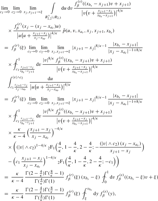
    where we also made the change of variables $y = (x_{b_{s}}-\xi )v+\xi$ to obtain the last line.

  The contribution of the integral over $R_{2,2}^- \cup R_{3,2}$ can be evaluated similarly by exchanging the roles of u and v, and the result is

  

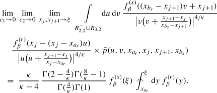  (C15)

Collecting all contributions, we finally obtain

Using also the functional equation $\Gamma (1-\nu )\Gamma (\nu )=\frac{\pi }{\sin (\pi \nu )}$, we find the multiplicative constant

$$\begin{aligned} \frac{\kappa }{\kappa -4} \, \frac{\Gamma (2-\frac{4}{\kappa }) \Gamma (\frac{8}{\kappa }-1)}{\Gamma (\frac{4}{\kappa })} \,=\frac{\Gamma (1-4/\kappa )^2}{\sqrt{q(\kappa )} \, \Gamma (2-8/\kappa )} . \end{aligned}$$

This completes the proof. $\square$

Proof of Proposition C.1, Case B

Define $\beta _B:= \beta {\setminus } (\{a_{s}, j\}\cup \{a_{r},j+1\})$ (we do not relabel the indices here), and denote by $\Gamma _{\beta _B}$ the integration contours in $\mathcal {H}_{\beta }$ other than $(x_{a_s}, x_j)$, $(x_{a_r},x_{j+1})$. Then, we have

(C16)

where, as in the proof of Case A, $f_\beta (\varvec{x}; \varvec{\ddot{u}})$ is a part of the integrand function (1.6) chosen to be real and positive on (C3), and where $I_B(x_{a_r}, x_{a_{s}}, x_j, x_{j+1}) =: I_B$ is the integral

with $x_{a_{s}}< {\text {Re}}(u_{s})< x_j< x_{a_{r}}< {\text {Re}}(u_{r}) < x_{j+1}$, where the branch of $(u_{s}-u_{r})^{8/\kappa }$ is chosen to be positive when ${\text {Re}}(u_{r}) < {\text {Re}}(u_{s})$, and, as before, $f_\beta ^{(r)}$ and $f_\beta ^{(s)}$ are the multivalued functions with branch choices (C5) and (C6), respectively. Note that for any fixed $\varvec{\ddot{x}} \in \mathfrak {X}_{2N-2}$ and $\varvec{\ddot{u}} \in \Gamma _{\beta _B}$, we have

$$\begin{aligned} f_\beta ^{(s)}(x) \, f_\beta ^{(r)}(y) = f_\beta ^{(s)}(y) \, f_\beta ^{(r)}(x) , \end{aligned}$$

for all $x, y \notin \{ x_1, \ldots , x_{j-1}, x_{j+2}, \ldots , x_{2N}, u_1, \ldots , u_{r-1}, u_{r+1}, \ldots , u_{s-1}, u_{s+1}, \ldots , u_N \}$ such that $x \ne y$, since the phase factors from the exchange of x and y in the product cancel out.

We proceed similarly as in the proof of Case A. After making the changes of variables $w=-\frac{x_{j+1}-u_{r}}{x_{j+1}-x_{a_{r}}}$ in the first integral and $u=\frac{x_j-u_{s}}{x_j-x_{a_{s}}}$ in the second integral, we obtain

where

$$\begin{aligned} \;&p(u, v, x_{a_r}, x_{a_{s}}, x_j, x_{j+1}) \\&\quad := \; \frac{\big ( x_{j+1} - x_j + u \, (x_j-x_{a_{s}}) + w \, (x_{j+1} - x_{a_{r}})\big )^{8/\kappa }}{| x_{a_{r}}-x_{j+1} |^{-1+8/\kappa } \, | x_j-x_{a_{s}} |^{-1+8/\kappa }} \\ \nonumber&\quad = \; \frac{\big ( u \, (x_j-x_{a_{s}}) + w \, (x_{j+1} - x_{a_{r}}) \big )^{8/\kappa }}{| x_{a_{r}}-x_{j+1} |^{-1+8/\kappa } \, | x_j-x_{a_{s}} |^{-1+8/\kappa }} + \mathcal {O}( |x_{j+1} - x_j| ) , \quad |x_{j+1} - x_j| \rightarrow 0 . \end{aligned}$$

This integral has a similar form as for $I_A$ defined in (C4), except for the following changes:

• $x_{a_{r}}$ in $I_B$ plays the role of $x_{b_{s}}$ in $I_A$;

• $x_{a_{s}}$ in $I_B$ plays the role of $x_{a_{r}}$ in $I_A$;

• in $I_B$, we have $x_{j+1}-x_{a_{r}} > 0$, while in $I_A$, we have $x_{b_{s}}-x_{j+1} > 0$;

• we integrate in $I_B$ the variable $w \in (-1,0)$, while in $I_A$ the corresponding variable is $v \in (0,1)$.

Nevertheless, this only affects the estimates slightly, so with similar estimates as in the proof of Case A, one can show that

(C17)

We then conclude from (C16) and (C17) that (C1) holds:

after carefully collecting the phase factors (and recalling that $\xi \in (x_{j-1}, x_{j+2})$ and that $f_\beta (\varvec{x}; \varvec{\ddot{u}})$ is real and positive on (C3), $f_\beta ^{(r)}$ is real and positive on (C5), and $f_\beta ^{(s)}$ is real and positive on (C6)). $\square$

Proof of Proposition C.1, Case C

This symmetric to Case B and can be proven very similarly. $\square$

References

Ang, M., Sun, X.: Integrability of the conformal loop ensemble (2021). arXiv:2107.01788
Abramowitz, M., Stegun, I.A.: Handbook of Mathematical Functions with Formulas, Graphs, and Mathematical Tables. Dover Publications Inc, New York (1992)
Bauer, M., Bernard, D., Kytölä, K.: Multiple Schramm–Loewner evolutions and statistical mechanics martingales. J. Stat. Phys. 120(5–6), 1125–1163 (2005)
Beffara, V., Duminil-Copin, H.: The self-dual point of the two-dimensional random-cluster model is critical for \(q\ge 1\). Probab. Theory Relat. Fields. 153(3–4), 511–542 (2012)
Beffara, V., Peltola, E., Wu, H.: On the uniqueness of global multiple SLEs. Ann. Probab. 49(1), 400–434 (2021)
Belavin, A.A., Polyakov, A.M., Zamolodchikov, A.B.: Infinite conformal symmetry in two-dimensional quantum field theory. Nucl. Phys. B 241(2), 333–380 (1984)
Belavin, A.A., Polyakov, A.M., Zamolodchikov, A.B.: Infinite conformal symmetry of critical fluctuations in two dimensions. J. Stat. Phys. 34(5–6), 763–774 (1984)
Cardy, J.L.: Conformal invariance and surface critical behavior. Nucl. Phys. B 240(4), 514–532 (1984)
Cardy, J.L.: Critical percolation in finite geometries. J. Phys. A. 25(4), L201-206 (1992)
Cardy, J.L.: Scaling and Renormalization in Statistical Physics, vol. 5 of Cambridge Lecture Notes in Physics. Cambridge University Press, Cambridge (1996)
Chelkak, D., Duminil-Copin, H., Hongler, C., Kemppainen, A., Smirnov, S.: Convergence of Ising interfaces to Schramm’s SLE curves. C. R. Math. Acad. Sci. Paris. 352(2), 157–161 (2014)
Chelkak, D., Duminil-Copin, H., Hongler, C.: Crossing probabilities in topological rectangles for the critical planar FK-Ising model. Electron. J. Probab. 21, 5 (2016)
Chelkak, D., Hongler, C., Izyurov, K.: Conformal invariance of spin correlations in the planar Ising model. Ann. Math. 181(3), 1087–1138 (2015)
Chelkak, D., Hongler, C., Izyurov, K.: Correlations of primary fields in the critical Ising model (2021). arXiv:2103.10263
Chelkak, D., Smirnov, S.: Discrete complex analysis on isoradial graphs. Adv. Math. 228(3), 1590–1630 (2011)
Chelkak, D., Smirnov, S.: Universality in the 2D Ising model and conformal invariance of fermionic observables. Invent. Math. 189(3), 515–580 (2012)
Chelkak, D., Wan, Y.: On the convergence of massive loop-erased random walks to massive SLE(2) curves. Electron. J. Probab. 26, 54 (2021)
Chelkak, D.: Ising model and s-embeddings of planar graphs (2020). arXiv:2006.14559
Duminil-Copin, H.: Lectures on the Ising and Potts models on the hypercubic lattice. In: PIMS-CRM Summer School in Probability, pp. 35–161. Springer, Berlin (2017)
Duminil-Copin, H., Hongler, C., Nolin, P.: Connection probabilities and RSW-type bounds for the two-dimensional FK-Ising model. Commun. Pure Appl. Math. 64(9), 1165–1198 (2011)
Duminil-Copin, H., Kozlowski, K.K., Krachun, D., Manolescu, I., Oulamara, M.: Rotational invariance in critical planar lattice models (2020). arXiv:2012.11672
Duminil-Copin, H., Manolescu, I., Tassion, V.: Planar random-cluster model: fractal properties of the critical phase. Probab. Theory Relat. Fields 181(1–3), 401–449 (2021)
Duminil-Copin, H., Smirnov, S.: Conformal invariance of lattice models. In: Probability and Statistical Physics in Two and More Dimensions, vol. 15 of Clay Mathematics Proceedings, pp. 213–276. American Mathematical Society, Providence, RI (2012)
Duminil-Copin, H., Sidoravicius, V., Tassion, V.: Continuity of the phase transition for planar random-cluster and Potts models with \(1\le q\le 4\). Commun. Math. Phys. 349(1), 47–107 (2017)
Duminil-Copin, H., Gagnebin, M., Harel, M., Manolescu, I., Tassion, V.: Discontinuity of the phase transition for the planar random-cluster and Potts models with \(q>4\). Ann. Sci. de l’Ecole Norm. Superieure. 6(54), 1363–1413 (2021)
Dotsenko, V.S., Fateev, V.A.: Conformal algebra and multipoint correlation functions in 2D statistical models. Nucl. Phys. B 240(3), 312–348 (1984)
Di Francesco, P., Golinelli, O., Guitter, E.: Meanders and the Temperley–Lieb algebra. Commun. Math. Phys. 186(1), 1–59 (1997)
Di Francesco, P., Mathieu, P., Sénéchal, D.: Conformal field theory. In: Graduate Texts in Contemporary Physics. Springer, New York (1997)
Delfino, G., Picco, M., Santachiara, R., Viti, J.: Connectivities of Potts Fortuin–Kasteleyn clusters and time-like Liouville correlator. Nucl. Phys. B 875(3), 719–737 (2013)
Dubédat, J.: Euler integrals for commuting SLEs. J. Stat. Phys. 123(6), 1183–1218 (2006)
Dubédat, J.: Commutation relations for Schramm–Loewner evolutions. Commun. Pure Appl. Math. 60(12), 1792–1847 (2007)
Flores, S.M., Kleban, P.: A solution space for a system of null-state partial differential equations: part 2. Commun. Math. Phys. 333(1), 435–481 (2015)
Flores, S.M., Kleban, P.: A solution space for a system of null-state partial differential equations: part 3. Commun. Math. Phys. 333(2), 597–667 (2015)
Flores, S.M., Kleban, P.: A solution space for a system of null-state partial differential equations: part 4. Commun. Math. Phys. 333(2), 669–715 (2015)
Flores, S.M., Peltola, E.: Standard modules, radicals, and the valenced Temperley–Lieb algebra (2018). arXiv:1801.10003
Flores, S.M., Kleban, P., Simmons, J.J.H., Ziff, R.M.: Cluster densities at 2D critical points in rectangular geometries. J. Phys. A. 44(38), 385002 (2011)
Flores, S.M., Kleban, P., Simmons, J.J.H., Ziff, R.M.: A formula for crossing probabilities of critical systems inside polygons. J. Phys. A. 50(6), 064005, 91 (2017)
Garban, C., Pete, G., Schramm, O.: Pivotal, cluster, and interface measures for critical planar percolation. J. Am. Math. Soc. 26(4), 939–1024 (2013)
Garban, C., Wu, H.: On the convergence of FK-Ising percolation to SLE(16/3, 16/3-6). J. Theor. Probab. 33, 828–865 (2020)
Grimmett, G.: The Random-Cluster Model. Springer, Berlin (2006)
Izyurov, K.: Smirnov’s observable for free boundary conditions, interfaces and crossing probabilities. Commun. Math. Phys. 337(1), 225–252 (2015)
Izyurov, K.: On multiple SLE for the FK-Ising model. Ann. Probab. 50(2), 771–790 (2022)
Junnila, J., Saksman, E., Webb, C.: Imaginary multiplicative chaos: Moments, regularity, and connections to the Ising model. Ann. Appl. Probab. 30(5), 2099–2164 (2020)
Karrila, A.: Limits of conformal images and conformal images of limits for planar random curves (2018). arXiv:1810.05608
Karrila, A.: Multiple SLE type scaling limits: from local to global (2019). arXiv:1903.10354
Karrila, A.: UST branches, martingales, and multiple SLE(2). Electron. J. Probab. 25, 83 (2020)
Kenyon, R.W.: Conformal invariance of domino tiling. Ann. Probab. 28(2), 759–795 (2000)
Karrila, A., Kytölä, K., Peltola, E.: Boundary correlations in planar LERW and UST. Commun. Math. Phys. 376(3), 2065–2145 (2020)
Kenyon, R.W., Wilson, D.B.: Boundary partitions in trees and dimers. Trans. Am. Math. Soc. 363(3), 1325–1364 (2011)
Kytölä, K., Peltola, E.: Pure partition functions of multiple SLEs. Commun. Math. Phys. 346(1), 237–292 (2016)
Kytölä, K., Peltola, E.: Conformally covariant boundary correlation functions with a quantum group. J. Eur. Math. Soc. 22(1), 55–118 (2020)
Kemppainen, A., Smirnov, S.: Conformal invariance in random-cluster models. II. Full scaling limit as a branching SLE (2016). arXiv:1609.08527
Kemppainen, A., Smirnov, S.: Random curves, scaling limits and Loewner evolutions. Ann. Probab. 45(2), 698–779 (2017)
Kemppainen, A., Smirnov, S.: Configurations of FK-Ising interfaces and Hypergeometric SLE. Math. Res. Lett. 25(3), 875–889 (2018)
Kemppainen, A., Smirnov, S.: Conformal invariance of boundary touching loops of FK-Ising model. Commun. Math. Phys. 369(1), 49–98 (2019)
Lawler, G.F.: Conformally Invariant Processes in the Plane, vol. 114 of Mathematical Surveys and Monographs. American Mathematical Society, Providence, RI (2005)
Langlands, R., Pouliot, P., Aubin, Y.S.: Conformal invariance in two-dimensional percolation. Bull. Am. Math. Soc. 30(1), 1–61 (1994)
Liu, M., Peltola, E., Wu, H.: Uniform spanning tree in topological polygons, partition functions for SLE(8), and correlations in \(c=-2\) logarithmic CFT. Ann. Probab. (2024, to appear). arXiv:2108.04421
Liu, M., Wu, H.: Scaling limits of crossing probabilities in metric graph GFF. Electron. J. Probab. 26, 37, 46 (2021)
Miller, J., Werner, W.: Connection probabilities for conformal loop ensembles. Commun. Math. Phys. 362(2), 415–453 (2018)
Pommerenke, C.: Boundary Behaviour of Conformal Maps, vol. 299 of Grundlehren der Mathematischen Wissenschaften. Springer, Berlin (1992)
Peltola, E., Wu, H.: Global and local multiple SLEs for \(\kappa \le 4\) and connection probabilities for level lines of GFF. Commun. Math. Phys. 366(2), 469–536 (2019)
Peltola, E.: Towards a conformal field theory for Schramm–Loewner evolutions. J. Math. Phys. 60(10), 103305 (2019)
Peltola, E., Wu, H.: Crossing probabilities of multiple percolation interfaces: generalizations of Cardy’s formula and Watt’s formula. In preparation (2024)
Rohde, S., Schramm, O.: Basic properties of SLE. Ann. Math. 161(2), 883–924 (2005)
Schramm, O., Smirnov, S.: On the scaling limits of planar percolation. With an appendix by Christophe Garban. Ann. Probab. 39(5), 1768–1814 (2011)
Schramm, O., Wilson, D.B.: SLE coordinate changes. N. Y. J. Math. 11, 659–669 (2005)
Smirnov, S.: Critical percolation in the plane: conformal invariance, Cardy’s formula, scaling limits. C. R. Acad. Sci. 333(3), 239–244 (2001)
Smirnov, S.: Conformal invariance in random-cluster models. I. Holomorphic fermions in the Ising model. Ann. Math. 172(2), 1435–1467 (2010)
Wu, H.: Hypergeometric SLE: conformal Markov characterization and applications. Commun. Math. Phys. 374(2), 433–484 (2020)
Acknowledgements
This material is part of a project that has received funding from the European Research Council (ERC) under the European Union’s Horizon 2020 research and innovation programme (101042460): ERC Starting grant “Interplay of structures in conformal and universal random geometry” (ISCoURaGe) and from the Academy of Finland grant number 340461 “Conformal invariance in planar random geometry.” E.P. is also supported by the Academy of Finland Centre of Excellence Programme grant number 346315 “Finnish centre of excellence in Randomness and STructures (FiRST)” and by the Deutsche Forschungsgemeinschaft (DFG, German Research Foundation) under Germany’s Excellence Strategy EXC-2047/1-390685813, as well as the DFG collaborative research centre “The mathematics of emerging effects” CRC-1060/211504053. Part of this work was carried out while E.P. participated in a program hosted by the Mathematical Sciences Research Institute (MSRI) in Berkeley, California, during Spring 2022, thereby being supported by the National Science Foundation under grant number DMS-1928930. H.W. is supported by Beijing Natural Science Foundation (JQ20001). H.W. is partly affiliated at Yanqi Lake Beijing Institute of Mathematical Sciences and Applications, Beijing, China. We thank Konstantin Izyurov for several discussions related to this work. We thank the anonymous referee for careful reading and helpful suggestions to improve this article.
Author information
Authors and Affiliations
Corresponding author
Ethics declarations
Conflict of interest
The authors have no competing interests to declare that are relevant to the content of this article.
Additional information
Publisher's Note
Springer Nature remains neutral with regard to jurisdictional claims in published maps and institutional affiliations.