A lower bound for the dimension of tetrahedral splines in large degree

Abstract

Splines are piecewise polynomial functions which are continuously differentiable to some order r. For a fixed integer d the space of splines of degree at most d is a finite dimensional vector space, and a largely open problem in numerical analysis is to determine its dimension. While considerable attention has been given to this problem in the bivariate setting, the literature on trivariate splines is less conclusive. In particular, the dimension of generic trivariate splines is not known even in large degree when $r>1$. In this paper we use a bound we previously derived for splines on vertex stars to compute a new lower bound on the dimension of trivariate splines in large enough degree. We illustrate in several examples that our formula gives the exact dimension of the spline space in large enough degree if vertex positions are generic. In contrast, for splines continuously differentiable of order $r>1$, every lower bound in the literature diverges (often significantly) in large degree from the dimension of the spline space in these examples. We derive the bound using commutative and homological algebra.

1 Introduction

A multivariate spline is a piecewise polynomial function on a partition $\Delta$ of some domain $\Omega \subset \mathbb {R}^n$ which is continuously differentiable to order r for some integer $r\ge 0$. Multivariate splines play an important role in many areas such as finite elements, computer-aided geometric design, isogeometric analysis, and data fitting [13, 24]. Splines on both triangulations and tetrahedral partitions have been used to solve boundary value problems by the finite element method; some early references are [14, 34, 35], see also [24] and the references therein. For quite recent applications in isogeometric analysis, in [18, 19], Engvall and Evans outline frameworks to parametrize volumes for isogeometric analysis using triangular and tetrahedral Bézier elements. While Engvall and Evans in [19] focus on $C^0$ elements, $C^r$ tetrahedral Bézier elements are also used for isogeometric analysis—see Xia and Qiang [38]. In these applications it is important to construct a basis, often with prescribed properties, for splines of bounded total degree. Thus it is important to compute the dimension of the space of multivariate splines of bounded degree on a fixed partition. We write $\mathcal {S}^r_d(\Delta )$ for the vector space of piecewise polynomial functions of degree at most d on the partition $\Delta$ which are continuously differentiable of order r. By an abuse of notation we identify $\Delta$ with its embedding in $\mathbb {R}^n$.

A formula for the dimension of $C^1$ splines on triangulations was proposed by Strang [34] and proved for generic triangulations by Billera [9]. Subsequently the problem of computing the dimension of planar splines on triangulations has received considerable attention using a wide variety of techniques, see [3, 4, 9, 11, 22, 23, 31,32,33, 36, 37]. Alfeld and Schumaker show in [4] that the dimension of $\mathcal {S}^r_d(\Delta )$, for (most) planar triangulations $\Delta$ and $d\ge 3r+1$, is given by a quadratic polynomial in d whose coefficients are determined from simple data of the triangulation. The computation of $\dim \mathcal {S}^r_d(\Delta )$ for planar $\Delta$ when $r+1\le d\le 3r$ remains an open problem, although Whiteley has shown that there are only trivial splines on $\Delta$ in degrees at most $\frac{3r+1}{2}$ if $\Delta$ is generic with a triangular boundary [36]. (This result of Whiteley is an essential ingredient of our lower bound for trivariate splines.)

The literature on computing the dimension of trivariate splines on tetrahedral partitions is much less conclusive. The dimension has been computed if $r=0$ (see [6] or [10]), and also if $r=1$, $d\ge 8$, and $\Delta$ is generic by Alfeld, Schumaker, and Whiteley [7]. For $r>1$ bounds on $\dim \mathcal {S}^r_d(\Delta )$ have been computed in [1, 5, 25, 28]. A major difficulty is that computing $\dim \mathcal {S}^r_d(\Delta )$ exactly in large degree for arbitrary tetrahedral partitions cannot be done without computing the dimension of splines on planar triangulations exactly in all degrees (see [7, Remark 65]). More precisely, to compute $\dim \mathcal {S}^r_d(\Delta )$ exactly for $d\gg 0$, we must be able to compute the space of homogeneous splines $\dim \mathcal {H}^r_d(\Delta _\gamma )$ exactly in all degrees, where $\gamma$ is a vertex of $\Delta$ and $\Delta _\gamma$ is the star of $\gamma$ (that is, $\Delta _\gamma$ consists of all tetrahedra having $\gamma$ as a vertex). The computation of such spline spaces has only been made for $r\le 1$; for $r=1$, the partition $\Delta$ is required to be generic [7]. For this crucial computation we rely on our previous paper [17], where we establish a lower bound on the dimension of homogeneous splines on vertex stars.

In our main result, Theorem 2.6, we establish a formula which is a lower bound on the dimension of the spline space on most tetrahedral partitions of interest (any triangulation of a compact three-manifold with boundary) in large enough degree. While we have no proof of what degree is large enough, empirical evidence suggests that, for generic $\Delta$, our formula begins to be a lower bound in degrees close to the initial degree of $\mathcal {S}^r(\Delta )$; by the initial degree of $\mathcal {S}^r(\Delta )$ we mean the smallest degree d in which $\mathcal {S}^r_d(\Delta )$ admits a spline which is not globally polynomial. If $\Delta$ is generic, our formula gives the exact dimension of $\mathcal {S}^r_d(\Delta )$ beginning at the initial degree of $\mathcal {S}^r_d(\Delta )$ for several tetrahedral partitions considered by Alfeld and Schumaker [5] (see Example 1.1 and Sect. 5). It is worth noting that none of the lower bounds in the literature [5, 25, 28] give the exact dimension of the generic spline space (even in large degree) on these tetrahedral partitions for $r\ge 2$. Below is an example, discussed in detail later in the paper, comparing our results to work by Alfeld and Schumaker in [5] and Mourrain and Villamizar in [28].

Example 1.1

Let $\Delta$ be the tetrahedral partition on the left of Figure 1. In Table 1 we record the values of the lower bounds on $\dim \mathcal {S}^r_d(\Delta )$ for order of smoothness $2\le r\le 4$. In column 3 we give the dimension of the space of polynomials of degree at most d (this is $\left( {\begin{array}{c}d+3\\ 3\end{array}}\right)$), in columns 4–6 the bounds are obtained by applying the formulas proved in [28, Theorem 5.1], [5, Example 8.2], and our new lower bound $\textrm{LB}(d)$ (proved in Theorem 2.6 below), respectively. The last column records the value for the exact dimension for the given order of continuity r, degree d, and generic vertex positions. The bolded entry in the d column indicates the initial degree of $\mathcal {S}^r_d(\Delta )$.

Fig. 1

A three-dimensional version of the Morgan–Scott triangulation, the star of the boundary vertex $\gamma '$ (center), and the star of the interior vertex $\gamma$ (right)

Table 1 Lower bounds on $\dim \mathcal {S}^r_d(\Delta )$, where $\Delta$ is the three dimensional Morgan–Scott partition in Fig. 1; see Example 5.1. The initial degree is bolded

The paper is organized as follows. In Sect. 2 we explicitly state our lower bound in purely numerical terms allowing a straightforward application of the formula and illustrate in an example. In Sect. 3 we set up notation and give relevant homological background, and in Sect. 4 we prove the bound of Theorem 2.6. Section 5 is devoted to illustrating our bounds in a number of examples and comparing them to the bounds in [5, 28]. Finally, we give some concluding remarks in Sect. 6. We draw special attention to Remark 6.2, as we think it likely that work of Alfeld, Schumaker, and Sirvent [6] implies that our formula is a lower bound in degrees at least $8r+1$. Our methods are sufficiently different from [6] that we do not attempt to prove this here.

2 The lower bound

  Throughout we let $\Delta$ be a tetrahedral partition. We are more precise in Sect. 3; for now it is sufficient for the reader to think of a tetrahedral partition as a triangulation of a three-dimensional polytope. We use $\Delta _i$ and $\Delta ^\circ _i$ to denote the i-faces and interior i-faces (respectively) of $\Delta$. We put $f_i(\Delta )=|\Delta _i|$ and $f^\circ _i(\Delta )=|\Delta ^\circ _i|$ (if $\Delta$ is clear we simply write $f_i$ and $f^\circ _i$). We define the following data for each edge (Notation 2.1) and for each vertex of $\Delta$ (Notation 2.3).

Notation 2.1

For a given $r\ge 0$ and $\tau \in \Delta _1$,

• we define $t_\tau =\min \{n_\tau ,r+2\}$, where $n_\tau =\#\{\sigma \in \Delta _2:\tau \subset \sigma \}$ is the number of two-dimensional faces having $\tau$ as an edge;

• and the constants

  $$\begin{aligned}q_\tau = \biggl \lfloor \frac{t_\tau (r+1)}{t_\tau -1}\biggr \rfloor ,\quad a_\tau =t_\tau (r+1)-(t_\tau -1) q_\tau \ , \text { and}\quad b_\tau =t_\tau -1-a_\tau \,.\end{aligned}$$

  Notice that $t_\tau (r+1)=q_\tau (t_\tau -1)+a_\tau$ ; i.e., $q_\tau$ and $a_\tau$ are, respectively, the quotient and remainder obtained when dividing $t_\tau (r+1)$ by $t_\tau -1$ .

Given a vertex $\gamma \in \Delta$, we call the set of tetrahedra of $\Delta$ which contain $\gamma$ the star of $\gamma$ and we denote this tetrahedral partition by $\Delta _\gamma$. If $\gamma$ is an interior vertex of $\Delta$, so $\gamma$ is completely surrounded by tetrahedra, then we call $\Delta _\gamma$ a closed vertex star. If $\gamma$ is a boundary vertex of $\Delta$, so $\gamma$ is not completely surrounded by tetrahedra, then we call $\Delta _\gamma$ an open vertex star.

The following convention for binomial coefficients is crucial in all our formulas.

Convention 2.2

For binomial coefficients we always put $\left( {\begin{array}{c}n\\ k\end{array}}\right) =0$ when $n<k$.

We make the following definitions following Notation 2.1 and Convention 2.2.

Notation 2.3

For given integers $d\ge r\ge 0$ and $\gamma \in \Delta _0$,

• if $\Delta _\gamma$ is a closed star i.e., $\gamma \in \Delta _0^\circ$, we define

  $$\begin{aligned} D_\gamma :=\left\{ \begin{array}{ll} 2r &{}\hbox {if} \quad f^\circ _1(\Delta _\gamma )=4\\ \lfloor (5r+2)/3 \rfloor &{}\hbox {if} \quad f_1^\circ (\Delta _\gamma )=5\\ \lfloor (3r+1)/2 \rfloor &{}\hbox {if} \quad f_1^\circ (\Delta _\gamma )\ge 6 , \end{array} \right. \end{aligned}$$

  (1)

  and

  

  (2)

  We write instead of if $\Delta$ and r are understood.

• If $\Delta _\gamma$ is an open vertex star i.e., if $\gamma \in \Delta _0\setminus \Delta _0^\circ$ , we define

  

  (3)

  Again we write if $\Delta$ and r are understood.

• For each vertex $\gamma \in \Delta _0$ we define the constant $N_\gamma$ as follows

  

  (4)

  where for a real number m, we put $[m]_+=\max \{m,0\}$. The constants $D_\gamma$, , and are those defined in Equations (1), (2), and (3), respectively.

Remark 2.4

In [17] we show is a lower bound for homogeneous splines on a generic closed vertex star for $d>D_\gamma$ and [2] shows there is equality for $d\ge 3r+2$. In [2] it is shown that is a lower bound for homogeneous splines on a generic open vertex star, with equality if $d\ge 3r+2$.

Remark 2.5

When $\gamma \in \Delta ^\circ _0$ and $r+1\le d\le D_\gamma$, notice that the contribution to $N_\gamma$ can be negative, while if $d>D_\gamma$, only positive contributions are counted. This is a crucial difference between the contributions from interior vertices and the contributions from boundary vertices.

Theorem 2.6

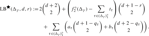
Suppose $\Delta$ is a tetrahedral partition. If $d\gg 0$ then $\dim \mathcal {S}^r_d(\Delta )\ge \textrm{LB}(\Delta ,d,r)$, where

$$\begin{aligned} \textrm{LB}(\Delta ,d,r) :=&\bigl (f_3-f^\circ _2+f^\circ _1\bigr )\left( {\begin{array}{c}d+3\\ 3\end{array}}\right) + \left( f^\circ _2-\sum \limits _{\tau \in \Delta ^\circ _1} t_\tau \right) \left( {\begin{array}{c}d+2-r\\ 3\end{array}}\right) \nonumber \\&+\sum \limits _{\tau \in \Delta ^\circ _1} \left( a_\tau \left( {\begin{array}{c}d+2-q_\tau \\ 3\end{array}}\right) +b_\tau \left( {\begin{array}{c}d+3-q_\tau \\ 3\end{array}}\right) \right) \nonumber \\&-f^\circ _0\left( {\begin{array}{c}r+3\\ 3\end{array}}\right) +\sum _{\gamma \in \Delta _0} N_\gamma \ . \end{aligned}$$

(5)

If $\Delta$ and r are understood then we abbreviate $\textrm{LB}(\Delta ,d,r)$ to $\textrm{LB}(d)$.

2.1 Example

We illustrate Theorem 2.6 for $C^2$ splines on the tetrahedral partition in Fig. 1, which is a three-dimensional analog of the Morgan–Scott triangulation [27]. If $\gamma$ is an interior vertex then $\Delta _\gamma$ is the triangulated octahedron on the right in Fig. 1. We have $f^\circ _0(\Delta _\gamma )=1$, $f^\circ _1(\Delta _\gamma )=6$, and $f^\circ _2(\Delta _\gamma )=12$. For every $\tau \in (\Delta _\gamma )_1^\circ$, we have $n_\tau =4$ and hence $t_\tau =\min \bigl \{n_\tau ,r+2\bigr \}=4$. We compute $q_\tau =4,a_\tau =0,$ and $b_\tau =3$, hence by Equation (2),

If $\gamma '$ is a boundary vertex, then $\Delta _{\gamma '}$ is the cone over the Morgan–Scott triangulation (see the star of vertex $\gamma '$ in Fig. 1). We have $f^\circ _0(\Delta _{\gamma '})=0$, $f^\circ _1(\Delta _{\gamma '})=3$, and $f^\circ _2(\Delta _{\gamma '})=9$. For every $\tau \in (\Delta _{\gamma '})_1^\circ$, we have $n_\tau =4$ and hence $t_\tau =\min \bigl \{n_\tau ,r+2\bigr \}=4$. Again we have $q_\tau =4,a_\tau =0,$ and $b_\tau =3$. Thus, following Equation (3),

In Table 2 we record the values of , , and $\left( {\begin{array}{c}d+2\\ 2\end{array}}\right)$ where $\gamma$ is an interior vertex of $\Delta$ and $\gamma '$ is a boundary vertex of $\Delta$.

Table 2 Lower bounds for the star of an interior ($\gamma$) and boundary ($\gamma '$) vertex of the simplicial complex in Fig. 1

Now we turn to computing the bound $\textrm{LB}\bigl (\Delta ,d,2\bigr )$ in Theorem 2.6 for $\dim \mathcal {S}^2_d(\Delta )$, where $\Delta$ is the full simplicial complex depicted in Fig. 1. If $\gamma$ is a boundary vertex then $N_\gamma =3$ (corresponding to the one difference in degree 3 in Table 2). If $\gamma$ is an interior vertex then $D_\gamma =3$. Reading down each column in the first two rows of Table 2 we get $N_\gamma =(10-8)+(15-12)=5$. Thus $\sum _{\gamma \in \Delta _0} N_\gamma =4\cdot 3+4\cdot (5)=32$.

For the remaining statistics we have $f_0^\circ =4,f_1^\circ =18,f_2^\circ =28,$ and $f_3=15$. For each interior 1-face $\tau$ we have $n_\tau =t_\tau =4, d_\tau =4, a_\tau =0, b_\tau =3$. Thus, by Theorem 2.6,

$$\begin{aligned} \textrm{LB}(\Delta ,d,2){=} 5\left( {\begin{array}{c}d+3\\ 3\end{array}}\right) -44\left( {\begin{array}{c}d\\ 3\end{array}}\right) +54\left( {\begin{array}{c}d-1\\ 3\end{array}}\right) -8 {=} \frac{5}{2}d^3-27d^2+\frac{187}{2}d-57, \end{aligned}$$

where the second equality holds as long as $d\ge 1$. Table 3 compares the values of $\textrm{LB}(\Delta ,d,2)$ and $\dim \mathcal {S}^2_d(\Delta )$ for generic positions of the vertices of $\Delta$. Notice that while $\textrm{LB}(\Delta ,d,2)$ is neither an upper or lower bound for $d\le 6$, it predicts the correct dimension of the generic spline space for $d\ge 7$. Incidentally, $d=7$ is the initial degree of $\mathcal {S}^2(\Delta )$; that is, the first non-trivial splines appear in degree 7. We computed the exact dimension of the spline space for generic vertex positions using the Algebraic Splines package in Macaulay2 [20]. Furthermore, a computation in Macaulay2 shows that $\dim \mathcal {S}^r_d(\Delta )=\frac{5}{2}d^3-27d^2+\frac{187}{2}d-57$ for $d\gg 0$, so our lower bound gives the exact dimension of the spline space for $r=2$ when $d\ge 7$. Code to compute all examples in this paper can be found on the first author’s website under the Research tab: https://midipasq.github.io/.

Table 3 Illustrating Theorem 2.6 for the tetrahedral partition in Fig. 1

3 Background and homological methods

In this section we introduce the homological methods of Billera [9] and Schenck and Stillman [32]. A simplex in $\mathbb {R}^n$ is the convex hull of $i\le n+1$ vertices which are in linearly general position (no three on a line, no four on a plane, etc.). A face of a simplex is the convex hull of any subset of the vertices which define it (thus a face of a simplex is a simplex). An i-simplex (or i-face) is the convex hull of $i+1$ vertices in linearly general position; i is the dimension of the i-simplex or i-face.

Definition 3.1

A simplicial complex $\Delta$ is a collection of simplices in $\mathbb {R}^n$ satisfying:

• If $\beta \in \Delta$ then so are all of its faces.

• If $\beta _1,\beta _2\in \Delta$ then $\beta _1\cap \beta _2$ is either empty or a proper face of both $\beta _1$ and $\beta _2$.

We also refer to the simplices of $\Delta$ as faces of $\Delta$. The dimension of $\Delta$ is the dimension of a maximal simplex of $\Delta$ under inclusion. If all maximal simplices have equal dimension we say that $\Delta$ is pure.

In this paper we only consider finite simplicial complexes. If $\beta$ is a face of $\Delta$ of dimension i we call $\beta$ an i-face. Denote by $\Delta _i$ and $\Delta _i^\circ$ the set i-faces of $\Delta$ and interior i-faces of $\Delta$, respectively. We write $f_i(\Delta )$ and $f^\circ _i(\Delta )$ for the number of i-faces and interior i-faces, respectively (we write $f_i$ and $f^\circ _i$ if $\Delta$ is understood). By an abuse of notation, we will identify $\Delta$ with its underlying space $\bigcup _{\beta \in \Delta } \beta \subset \mathbb {R}^n$.

Definition 3.2

If $\Delta$ is a simplicial complex and $\beta$ is a face of $\Delta$, then the link of $\beta$ is the set of all simplices $\gamma$ in $\Delta$ so that $\beta \cap \gamma =\emptyset$ and $\beta \cup \gamma$ is a face of $\Delta$. The star of $\beta$ is the union of the link of $\beta$ with the set of all simplices which contain $\beta$ (including $\beta$). We denote the star of $\beta$ by $\Delta _\beta$.

If $\gamma$ is a vertex of a simplicial complex $\Delta$ so that all maximal simplices of $\Delta$ contain $\gamma$ (so $\Delta _\gamma =\Delta$), then we call $\Delta$ the star of $\gamma$ and we say $\Delta$ is a vertex star. If $\gamma$ is an interior vertex we call $\Delta$ a closed vertex star and if $\gamma$ is a boundary vertex then we call $\Delta$ an open vertex star.

We refer to the set of points in $\mathbb {R}^{n+1}$ of unit norm as the n-sphere, and the set of points in $\mathbb {R}^n$ with norm at most one as the n-disk. A homeomorphism $f:X\rightarrow Y$ between two sets is a continuous bijection; if such an f exists we say X and Y are homeomorphic.

Definition 3.3

(Simplicial n-manifold with boundary) If $\Delta$ is a finite simplicial complex in $\mathbb {R}^n$, we say it is a simplicial n-manifold with boundary if it satisfies the conditions:

• $\Delta$ is pure n-dimensional,

• the link of every vertex of $\Delta$ is homeomorphic to an $(n-1)$-sphere (if the vertex is interior) or an $(n-1)$-disk (if the vertex is on the boundary),

• and every $(n-1)$-simplex of $\Delta$ is either the intersection of two n-simplices of $\Delta$ or it is on the boundary of $\Delta$ and so contained in only one n-simplex of $\Delta$.

Example 3.4

Consider the simplicial complex in Fig. 1, which is a simplicial 3-manifold with boundary homeomorphic to the 3-disk. The star of the interior vertex $\gamma$ is shown in the center of Fig. 1; the link of the vertex $\gamma$ is obtained from the star of $\gamma$ by removing $\gamma$ and all simplices which contain it. The link of $\gamma$ is homeomorphic to a 2-sphere. Likewise, the star of the boundary vertex $\gamma '$ is shown on the right in Fig. 1; the link of the vertex $\gamma '$ is obtained from it by removing the vertex $\gamma '$ and all simplices which contain it. The link of $\gamma '$ is the usual planar Morgan–Scott configuration [27], and is homeomorphic to a 2-disk.

Throughout this paper we abuse notation by referring to a simplicial n-manifold with boundary simply as a simplicial complex. We refer to a simplicial 2-manifold with boundary as a triangulation and a simplicial 3-manifold with boundary as a tetrahedral partition.

Write $\texttt{S}=\mathbb {R}[x_1,\ldots ,x_n]$ for the polynomial ring in n variables and $\texttt{S}_{\le d}$ for the $\mathbb {R}$-vector space of polynomials of total degree most d, and $\texttt{S}_d$ for the $\mathbb {R}$-vector space of polynomials which are homogeneous of degree exactly d. For a fixed integer r, we denote by $C^r(\Delta )$ the set of all functions $F: \Delta \rightarrow \mathbb {R}$ which are continuously differentiable of order r.

Definition 3.5

Let $\Delta \subset \mathbb {R}^n$ be an n-dimensional simplicial complex. We denote by

$$\begin{aligned} \mathcal {S}^r(\Delta ):= \bigl \{F\in C^r(\Delta ):F|_\iota \in \texttt{S}\; \hbox { for all }\iota \in \Delta _n \bigr \} \end{aligned}$$

the vector space of splines which are continuously differentiable of order r, by

$$\begin{aligned} \mathcal {S}^r_d(\Delta ):= \bigl \{F\in C^r(\Delta ):F|_\iota \in \texttt{S}_{\le d}\; \hbox { for all }\iota \in \Delta _n \bigr \} \end{aligned}$$

the subspace of $\mathcal {S}^r(\Delta )$ consisting of splines of degree at most d, and by

$$\begin{aligned} \mathcal {H}^r_d(\Delta ):= \bigl \{F\in C^r(\Delta ):F|_\iota \in \texttt{S}_d\; \hbox { for all }\iota \in \Delta _n\bigr \} \end{aligned}$$

the subspace of $\mathcal {S}^r(\Delta )$ consisting of splines whose restriction to each n-dimensional simplex is a homogeneous polynomial of degree d. We call splines in $\mathcal {H}^r_d(\Delta )$ homogeneous splines.

Suppose $\Delta$ is the star of a vertex. By changing coordinates, we will assume that this vertex is the origin in $\mathbb {R}^n$. Then one can show that

$$\begin{aligned} \mathcal {S}^r(\Delta )\cong \bigoplus \limits _{i\ge 0} \mathcal {H}^r_i(\Delta ), \hbox { and}\quad \mathcal {S}^r_d(\Delta )\cong \bigoplus \limits _{i=0}^d \mathcal {H}^r_i(\Delta ), \end{aligned}$$

(6)

where the isomorphism is as $\mathbb {R}$-vector spaces. We refer to the first isomorphism in (6) as the graded structure of $\mathcal {S}^r(\Delta )$. If $\Delta$ is not the star of a vertex, then (6) does not hold for $\mathcal {S}^r(\Delta )$; we summarize a coning construction of Billera and Rose under which (6) will still be valid.

Construction 3.6

Let $\mathbb {R}^n$ have coordinates $x_1,\ldots ,x_n$, $\mathbb {R}^{n+1}$ have coordinates $x_0,\ldots ,x_n$, and define $\phi :\mathbb {R}^n\rightarrow \mathbb {R}^{n+1}$ by $\phi (x_1,\ldots ,x_n)=(1,x_1,\ldots ,x_n)$. If $\sigma$ is a simplex in $\mathbb {R}^n$, the cone over $\sigma$, denoted $\widehat{\sigma }$, is the simplex in $\mathbb {R}^{n+1}$ which is the convex hull of the origin in $\mathbb {R}^{n+1}$ and $\phi (\sigma )$. If $\Delta \subset \mathbb {R}^n$ is a simplicial complex, the cone over $\Delta$, denoted $\widehat{\Delta }$, is the simplicial complex consisting of the simplices $\bigl \{\widehat{\beta }:\beta \in \Delta \bigr \}$ along with the origin in $\mathbb {R}^{n+1}$, which is called the cone vertex. We denote the polynomial ring $\mathbb {R}[x_0,x_1,\ldots ,x_n]$ associated to $\widehat{\Delta }$ by $\widehat{\texttt{S}}$.

For any simplicial complex $\Delta \subset \mathbb {R}^n$, the simplicial complex $\widehat{\Delta }\subset \mathbb {R}^{n+1}$ is an (open) vertex star of the cone vertex. Thus (6) yields $\mathcal {S}^r(\widehat{\Delta })\cong \bigoplus \limits _{i\ge 0} \mathcal {H}^r_i(\widehat{\Delta }) \hbox { and } \mathcal {S}^r_d(\widehat{\Delta })\cong \bigoplus \limits _{i=0}^d \mathcal {H}^r_i(\widehat{\Delta }).$ Moreover, Billera and Rose show that

Theorem 3.7

[11, Theorem 2.6] $\mathcal {S}^r_d(\Delta )\cong \mathcal {H}^r_d(\widehat{\Delta })$.

Thus the study of spline spaces reduces to the study of homogeneous spline spaces.

Definition 3.8

A subset $\texttt{I}\subset \texttt{S}$ is called an ideal if, for every $f,g\in \texttt{I}$ and $h\in \texttt{S}$, $f+g\in \texttt{I}$ and $hf\in \texttt{I}$. If $f_1,\ldots ,f_k\in \texttt{S}$ are polynomials, we write $\langle f_i \rangle$ for the vector space of all polynomial multiples of $f_i$ ($i=1,\ldots ,k$) and $\langle f_1,\ldots ,f_k\rangle :=\sum _{i=1}^k \langle f_i\rangle$. This is called the ideal generated by $f_1,\ldots ,f_k$. We typically only use its vector space structure.

Definition 3.9

Suppose $\Delta \subset \mathbb {R}^n$ is an n-dimensional simplicial complex. If $\beta \in \Delta _n$ we define $\texttt{J}(\beta )=0$. If $\sigma \in \Delta _{n-1}$, let $\ell _\sigma$ be a choice of linear form vanishing on $\sigma$. We define $\texttt{J}(\sigma )=\langle \ell _\sigma ^{r+1}\rangle$. For any face $\beta \in \Delta _i$ where $i<n$ we define

$$\begin{aligned} \texttt{J}(\beta ):=\sum _{\sigma \supseteq \beta } \texttt{J}(\sigma )=\langle \ell ^{r+1}_\sigma : \beta \subseteq \sigma \rangle . \end{aligned}$$

Billera and Rose show that if $\Delta$ is hereditary (a hypothesis which is implied by ours) then

Proposition 3.10

[11, Proposition 1.2] $F\in \mathcal {S}^r(\Delta )$ if and only if

$$\begin{aligned} F|_{\iota }-F|_{\iota '}\in \texttt{J}(\sigma ) \quad \hbox {for every }\iota , \iota '\in \Delta _n \quad \hbox { satisfying } \iota \cap \iota '=\sigma \in \Delta _{n-1}. \end{aligned}$$

3.1 Chain complexes

If $C_0,\ldots ,C_k$ are vector spaces and $\partial _i:C_i\rightarrow C_{i-1}$ ($i=1,\ldots ,k$) are linear maps satisfying $\partial _{i-1}\circ \partial _i=0$ (for $i=2,\ldots ,k$), then the collection of this data is called a chain complex; this is typically recorded as

$$\begin{aligned} \mathcal {C}: 0\rightarrow C_k \xrightarrow {\partial _k} C_{k-1}\xrightarrow {\partial _{k-1}}\cdots \xrightarrow {\partial _1} C_0\rightarrow 0. \end{aligned}$$

We call the subscript i of $C_i$ the homological index and refer to $C_i$ as the vector space of $\mathcal {C}$ in homological index i. The homologies of the chain complex are the quotient vector spaces $H_i(\mathcal {C})=\ker (\partial _{i})/\mathrm {im\,}(\partial _{i-1})$ for $i=0,\ldots ,k$. (We put $H_0(\mathcal {C})=C_0/\mathrm {im\,}(\partial _1)$ and $H_k(\mathcal {C})=\ker (\partial _k)$.) Often $H_*(\mathcal {C})$ is used to denote the entire set of homology groups $H_0(\mathcal {C}),\ldots ,H_k(\mathcal {C})$. We are primarily concerned with a topological construction of chain complexes; see [21, Chapter 2] for a standard reference.

We now define the chain complex introduced by Billera [9] and refined by Schenck and Stillman [32]. Let $\texttt{S}^{\Delta _i}$ ($i=0,\ldots ,n$) denote the direct sum $\bigoplus _{\beta \in \Delta _i} \texttt{S}[\beta ]$, where $[\beta ]$ is a formal basis symbol corresponding to the i-face $\beta$. Fix an ordering $\gamma _1,\ldots ,\gamma _{f_0}$ of the vertices of $\Delta$. Each i-face $\beta \in \Delta _i$ can be represented as an ordered list $\beta =(\gamma _{j_0},\ldots ,\gamma _{j_i})$ of $i+1$ vertices. We define the simplicial boundary map $\partial _i$ (for $i=1,2,3$) on the formal symbol $[\beta ]=[\gamma _{j_0},\ldots ,\gamma _{j_i}]$ by $\partial _i\bigl ([\beta ]\bigr )=\partial _i\bigl ([\gamma _{j_0},\ldots ,\gamma _{j_i}]\bigr )=\sum _{k=0}^i (-1)^i\bigl [\gamma _{j_0},\ldots ,\hat{\gamma }_{j_k},\ldots ,\gamma _{j_i}\bigr ]$, where $\hat{\gamma }_{j_k}$ means that the vertex $\gamma _{j_k}$ is omitted from the list. We extend this map linearly to $\bigoplus _{\beta \in \Delta _i} \texttt{S}[\beta ]$.

It is straightforward to verify that $\partial _{i-1}\circ \partial _i=0$ for $i=2,\ldots ,n$ (this only needs to be checked on the basis symbols $[\beta ]$). Clearly the simplicial boundary map $\partial _i$ can be restricted to a map $\partial _i: \texttt{S}^{\Delta ^\circ _i}\rightarrow \texttt{S}^{\Delta ^\circ _{i-1}}$ where all formal symbols corresponding to faces on the boundary of $\Delta$ are dropped. We denote by $\mathcal {R}[\Delta ]$ the chain complex

$$\begin{aligned} \mathcal {R}[\Delta ] :\quad 0\longrightarrow \texttt{S}^{\Delta _n}\xrightarrow {\partial _n} \texttt{S}^{\Delta ^\circ _{n-1}} \xrightarrow {\partial _{n-1}} \cdots \xrightarrow {\partial _2} \texttt{S}^{\Delta ^\circ _1} \xrightarrow {\partial _1} \texttt{S}^{\Delta ^\circ _0} \longrightarrow 0\ . \end{aligned}$$

(This is the simplicial chain complex of $\Delta$ relative to its boundary $\partial \Delta$ with coefficients in $\texttt{S}$—see [21, Chapter 2.1]).

We now put the vector spaces $\texttt{J}(\beta )$ together to make a sub-chain complex of $\mathcal {R}[\Delta ]$

$$\begin{aligned}{} & {} \mathcal {J}[\Delta ]:\quad 0\longrightarrow \bigoplus _{\iota \in \Delta _n} \texttt{J}(\iota )=0 \rightarrow \bigoplus _{\sigma \in \Delta ^\circ _{n-1}} \texttt{J}(\sigma )\xrightarrow {\partial _{n-1}}\cdots \xrightarrow {\partial _2}\\ {}{} & {} \qquad \bigoplus _{\tau \in \Delta ^\circ _1} \texttt{J}(\tau ) \xrightarrow {\partial _1} \bigoplus _{\gamma \in \Delta ^\circ _0} \texttt{J}(\gamma ) \longrightarrow 0. \end{aligned}$$

The Billera-Schenck-Stillman chain complex is the quotient of $\mathcal {R}[\Delta ]$ by $\mathcal {J}[\Delta ]$, namely

$$\begin{aligned}{} & {} \mathcal {R}/\mathcal {J}[\Delta ] :\quad 0\longrightarrow \bigoplus _{\iota \in \Delta _{n}} \texttt{S}\xrightarrow {\overline{\partial }_n} \bigoplus _{\sigma \in \Delta _{n-1}^\circ } \frac{\texttt{S}}{\texttt{J}(\sigma )}\xrightarrow {\overline{\partial }_{n-1}} \cdots \xrightarrow {\overline{\partial }_2}\\ {}{} & {} \qquad \bigoplus _{\tau \in \Delta _1^\circ }\frac{\texttt{S}}{\texttt{J}(\tau )}\xrightarrow {\overline{\partial }_1} \bigoplus _{\gamma \in \Delta _0^\circ }\frac{\texttt{S}}{\texttt{J}(\gamma )}\longrightarrow 0. \end{aligned}$$

Remark 3.11

If the simplicial complex $\Delta$ is fixed, we simply write $\mathcal {J},\mathcal {R},$ and $\mathcal {R}/\mathcal {J}$ for the chain complexes $\mathcal {J}[\Delta ],\mathcal {R}[\Delta ]$, and $\mathcal {R}/\mathcal {J}[\Delta ]$, respectively.

Notation 3.12

We introduce a natural abuse of notation regarding the coning construction 3.6. If $\Delta$ is a simplicial complex and $\widehat{\Delta }$ is the cone over $\Delta$, then $\widehat{\Delta }$ is an open vertex star. Hence there is no interior vertex of $\widehat{\Delta }$ and thus the vector space of homological index 0 in $\mathcal {J}[\widehat{\Delta }],\mathcal {R}[\widehat{\Delta }],$ and $\mathcal {R}/\mathcal {J}[\widehat{\Delta }]$ is just zero. We thus decrease the homological index by one of each of the vector spaces in $\mathcal {J}[\widehat{\Delta }],\mathcal {R}[\widehat{\Delta }],$ and $\mathcal {R}/\mathcal {J}[\widehat{\Delta }]$. Hence if $\Delta \subset \mathbb {R}^n$ and thus $\widehat{\Delta }\subset \mathbb {R}^{n+1}$, $H_n(\mathcal {R}/\mathcal {J}[\widehat{\Delta }])$ is the top homology of the chain complex $\mathcal {R}/\mathcal {J}[\widehat{\Delta }]$, not $H_{n+1}(\mathcal {R}/\mathcal {J}[\widehat{\Delta }])$ (and likewise for lower indices). Thus the vector space in homological index i ($0\le i\le n$) in $\mathcal {R}/\mathcal {J}[\widehat{\Delta }]$ corresponds to the homological index i in $\mathcal {R}/\mathcal {J}[\Delta ]$, so its summands are indexed by $\Delta ^\circ _i$.

The crucial observation of Billera is that $H_n(\mathcal {R}/\mathcal {J}[\Delta ])\cong \mathcal {S}^r(\Delta )$; this follows from the criterion of Proposition 3.10.

3.2 Graded structure

The vector space $\texttt{J}(\beta )$ is infinite-dimensional for each face $\beta \in \Delta$ which is not a tetrahedron. Thus the constituents of the chain complexes $\mathcal {J}[\Delta ],\mathcal {R}[\Delta ],$ and $\mathcal {R}/\mathcal {J}[\Delta ]$ are also infinite-dimensional. In order to get a chain complex of finite dimensional vector spaces to relate to the fundamental spaces of interest ($\mathcal {S}^r_d(\Delta )$ and $\mathcal {H}^r_d(\Delta )$), we make use of a graded structure.

Definition 3.13

Let V be a real vector space and suppose $V_i$ is a finite-dimensional vector subspace of V for every integer $i\ge 0$. If $V\cong \bigoplus _{i\ge 0} V_i$, then we refer to this isomorphism as a graded structure of V and we call V a graded vector space. In particular, if $\texttt{J}\subset \texttt{S}$ is an ideal (c.f. Definition 3.8), then we write $\texttt{J}_d$ for the vector space of homogeneous polynomials of degree d in $\texttt{J}$. If $\texttt{J}\cong \bigoplus _{d\ge 0} \texttt{J}_d$ then we call $\texttt{J}$ a graded ideal of $\texttt{S}$.

Definition 3.14

If $\mathcal {C}: 0\rightarrow C_n\xrightarrow {\partial _n}\cdots \xrightarrow {\partial _1} C_0 \rightarrow 0$ is a chain complex of vector spaces so that

• (1) The vector space $C_j$ has a graded structure $C_j\cong \bigoplus _{i\ge 0} (C_j)_i$ for $j=0,\ldots ,n$ and

• (2) The map $\partial _j:C_j\rightarrow C_{j-1}$ satisfies $\partial _j((C_j)_i)\subset (C_{j-1})_i$ for $j=1,\ldots ,n$ ,

then $\mathcal {C}_d:=0\rightarrow (C_n)_d\xrightarrow {\partial _n} (C_{n-1})_d \xrightarrow {\partial _{n-1}}\cdots \xrightarrow {\partial _1} (C_0)_d \rightarrow 0$ is a chain complex which we call the degree d strand of $\mathcal {C}$. In this case we say $\mathcal {C}$ is graded with graded structure $\mathcal {C}\cong \bigoplus _{d\ge 0} \mathcal {C}_d$.

If a chain complex $\mathcal {C}$ has a graded structure $\mathcal {C}\cong \bigoplus _{d\ge 0}\mathcal {C}_d$, it is straightforward to see that the homologies of $\mathcal {C}$ also have the graded structure $H_i(\mathcal {C})\cong \bigoplus _{d\ge 0} H_i(\mathcal {C})_d$, where $H_i(\mathcal {C})_d:= H_i(\mathcal {C}_d)$ is the ith homology of the degree d strand.

Remark 3.15

The isomorphisms (6) show that $\mathcal {S}^r(\Delta )$ has a graded structure if $\Delta$ is the star of a vertex where the vertex is at the origin in $\mathbb {R}^n$.

If $\Delta$ is a vertex star of $\gamma$ (which we can assume to be located at the origin, if necessary, by changing coordinates) and $\gamma \in \beta$, then the linear forms whose powers generate $\texttt{J}(\beta )$ have no constant term and $\texttt{J}(\beta )$ is a graded ideal. It is straightforward to see that the simplicial boundary map respects this graded structure (i.e. property (2) of Definition 3.14 is satisfied), so if $\Delta$ is a vertex star then the chain complexes $\mathcal {J}[\Delta ],\mathcal {R}[\Delta ],$ and $\mathcal {R}/\mathcal {J}[\Delta ]$ also have a graded structure, along with their homologies. In particular, $\mathcal {H}^r_d(\Delta )\cong H_n\bigl (\mathcal {R}/\mathcal {J}[\Delta ]\bigr )_d$ if $\Delta \subset \mathbb {R}^n$ is a vertex star. If $\Delta$ is not necessarily a vertex star, we use the coning construction $\Delta \rightarrow \widehat{\Delta }$. Then $\widehat{\Delta }$ is a vertex star (whose vertex is at the origin) and so $\mathcal {S}^r(\widehat{\Delta })$, along with $\mathcal {J}[\widehat{\Delta }],\mathcal {R}[\widehat{\Delta }],$ and $\mathcal {R}/\mathcal {J}[\widehat{\Delta }]$, all have a graded structure. Keeping in mind Theorem 3.7 and Notation 3.12, we have $\mathcal {S}^r_d(\Delta )\cong \mathcal {H}^r_d(\widehat{\Delta })\cong \ker (\overline{\partial }_n)_d\cong H_n\bigl (\mathcal {R}/\mathcal {J}[\widehat{\Delta }]\bigr )_d$.

3.3 Euler characteristic and dimension formulas

If $\mathcal {C}:0\rightarrow C_n\rightarrow C_{n-1} \rightarrow \cdots \rightarrow C_0\rightarrow 0$ is a chain complex with a graded structure, we write $\chi (\mathcal {C},d)=\sum _{i=0}^n (-1)^{n-i}\dim (C_i)_d$. This is the Euler-Poincaré characteristic of $\mathcal {C}_d$. The rank-nullity theorem yields:

$$\begin{aligned} \chi (\mathcal {C},d)=\sum _{i=0}^n (-1)^{n-i} \dim H_i(\mathcal {C})_d. \end{aligned}$$

(7)

The three chain complexes $\mathcal {J},\mathcal {R},$ and $\mathcal {R}/\mathcal {J}$ fit into the short exact sequence of chain complexes $0\rightarrow \mathcal {J}\rightarrow \mathcal {R}\rightarrow \mathcal {R}/\mathcal {J} \rightarrow 0$. Correspondingly there is the long exact sequence:

$$\begin{aligned} 0\rightarrow H_n(\mathcal {J})\rightarrow H_n(\mathcal {R}) \rightarrow { \cdots }\rightarrow H_1(\mathcal {R}/\mathcal {J}){\rightarrow } H_0(\mathcal {J}){\rightarrow } H_0(\mathcal {R})\rightarrow H_0(\mathcal {R}/\mathcal {J}){\rightarrow } 0. \end{aligned}$$

The short exact sequence $0\rightarrow \mathcal {J}\rightarrow \mathcal {R}\rightarrow \mathcal {R}/\mathcal {J}\rightarrow 0$ also yields

$$\begin{aligned} \chi (\mathcal {R}/\mathcal {J},d)=\chi (\mathcal {R},d)+\chi (\mathcal {J},d)\ . \end{aligned}$$

(8)

There is a sum instead of a difference on the right hand side of Equation (8) because the first non-zero term in the chain complex $\mathcal {J}$ has homological degree $n-1$ instead of n.

Proposition 3.16

For an n-dimensional simplicial complex $\Delta$ in $\mathbb {R}^n$, $H_n(\mathcal {R}/\mathcal {J}[\widehat{\Delta }])_d\cong \mathcal {S}^r_d(\Delta )$ and $H_0(\mathcal {R}/\mathcal {J}[\Delta ])=0$. If $\Delta$ is a vertex star, $H_n(\mathcal {R}/\mathcal {J}[\Delta ])_d\cong \mathcal {H}^r_d(\Delta )$. If $\Delta$ is connected, then $H_0(\mathcal {R}/\mathcal {J}[\Delta ])=0$. If $\Delta$ is a vertex star whose link is homeomorphic to an $(n-1)$-sphere or an $(n-1)$-disk, then $\mathcal {S}^r(\Delta )\cong H_n(\mathcal {R}/\mathcal {J})\cong \texttt{S}\oplus H_{n-1}(\mathcal {J})$ and $H_i(\mathcal {R}/\mathcal {J})\cong H_{i-1}(\mathcal {J})$ for $i=1,\ldots ,n-1$.

Proof

By Theorem 3.7 and Proposition 3.10, $\mathcal {S}^r_d(\Delta ) \cong \mathcal {H}^r_d(\widehat{\Delta }) \cong H_n(\mathcal {R}/\mathcal {J}[\Delta ])_d$. Since every vertex can be connected to the boundary of $\Delta$ by a path consisting of interior edges, $\partial _1:\texttt{S}^{f^\circ _1}\rightarrow \texttt{S}^{f^\circ _0}$ is surjective and thus $H_0(\mathcal {R}[\Delta ])=0$, hence $H_0(\mathcal {R}/\mathcal {J}[\Delta ])=0$ by the long exact sequence associated to $0\rightarrow \mathcal {J}\rightarrow \mathcal {R}\rightarrow \mathcal {R}/\mathcal {J}\rightarrow 0$ .

The hypothesis that $\Delta$ is a vertex star whose link is homeomorphic to an $(n-1)$-sphere or an $(n-1)$-disk implies that $H_i(\mathcal {R}[\Delta ])=0$ for $0\le i<n$ and $H_n(\mathcal {R}[\Delta ])\cong \texttt{S}$ (by excision [21, Proposition 2.22], the homology of $\Delta$ relative to its boundary coincides with the homology of the n-sphere, which gives the claimed homologies). Then the last result follows from the long exact sequence associated to $0\rightarrow \mathcal {J}\rightarrow \mathcal {R}\rightarrow \mathcal {R}/\mathcal {J}\rightarrow 0$. $\square$

Remark 3.17

If $\Delta$ is homeomorphic to an n-disk, then the copy of $\texttt{S}$ in $\mathcal {S}^r(\Delta )\cong \texttt{S}\oplus H_{n-1}(\mathcal {J})$ corresponds to the globally polynomial splines, while the so-called smoothing cofactors are encoded by the map

$$\begin{aligned} \bigoplus _{\sigma \in \Delta ^\circ _{n-1}} \texttt{J}(\sigma ) \xrightarrow {\partial _{n-1}} \bigoplus _{\tau \in \Delta ^\circ _{n-2}} \texttt{J}(\beta )\ . \end{aligned}$$

Proposition 3.18

If $\Delta$ is a tetrahedral partition then

$$\begin{aligned}{} & {} \dim \mathcal {S}^r_d(\Delta )=\bigl (f_3-f^\circ _2+f^\circ _1-f^\circ _0\bigr )\dim \widehat{\texttt{S}}_d+\chi \bigl (\mathcal {J}[\widehat{\Delta }],d\bigr )\nonumber \\{} & {} \quad +\dim H_2\bigl (\mathcal {R}/\mathcal {J}[\widehat{\Delta }]\bigr )_d- \dim H_1\bigl (\mathcal {R}/\mathcal {J}[\widehat{\Delta }]\bigr )_d. \end{aligned}$$

(9)

If $\Delta$ is a tetrahedral vertex star whose link is homeomorphic to a 2-sphere or a 2-disk then

$$\begin{aligned} \dim \mathcal {H}^r_d(\Delta )=\dim \texttt{S}_d+\chi (\mathcal {J}[\Delta ],d)+\dim H_1(\mathcal {J}[\Delta ])_d. \end{aligned}$$

(10)

Proof

First we make use of the identifications $\mathcal {S}^r_d(\Delta )\cong \mathcal {H}^r_d(\widehat{\Delta })$ and $H_3(\mathcal {R}/\mathcal {J}[\widehat{\Delta }])_d\cong \mathcal {H}^r_d(\widehat{\Delta })$ of Theorems 3.7 and Proposition 3.16 (using Notation 3.12 for the second isomorphism). The identity (7) applied to the Euler-Poincaré characteristic of $\mathcal {R}/\mathcal {J}[\widehat{\Delta }]$, coupled with Proposition 3.16, gives

$$\begin{aligned} \dim \mathcal {S}_d^r(\Delta ) = \chi (\mathcal {R}/\mathcal {J}[\widehat{\Delta }],d) +\dim H_2(\mathcal {R}/\mathcal {J}[\widehat{\Delta }])_d-\dim H_1(\mathcal {R}/\mathcal {J}[\widehat{\Delta }])_d. \end{aligned}$$

To get Equation (9), note that $\mathcal {R}$ has the form $0\rightarrow \texttt{S}^{f_3}\rightarrow \texttt{S}^{f^\circ _2}\rightarrow \texttt{S}^{f^\circ _1}\rightarrow \texttt{S}^{f^\circ _0}\rightarrow 0;$ taking the Euler characteristic in degree d and using Equation (8) yields Equation (9). For Equation (10), Proposition 3.16 implies that $\dim \mathcal {H}^r_d(\Delta )=\dim \texttt{S}_d + \dim H_2(\mathcal {J}[\Delta ])_d.$ Taking the Euler-Poincaré characteristic of $\mathcal {J}[\Delta ]$ gives

$$\begin{aligned} \dim H_2(\mathcal {J}[\Delta ])_d=\chi (\mathcal {J}[\Delta ],d)+\dim H_1(\mathcal {J}[\Delta ])_d- \dim H_0(\mathcal {J}[\Delta ])_d. \end{aligned}$$

It is straightforward to show that $H_0(\mathcal {J}[\Delta ])=0$; putting together the above two equations yields Equation (10). $\square$

3.4 Generic simplicial complexes

It is well-known that, for a fixed r and d, there is an open set in $(\mathbb {R}^{n})^{f_0}$ of vertex coordinates of $\Delta$ for which $\dim \mathcal {S}^r_d(\Delta )$ is constant.

Definition 3.19

Suppose $\Delta$ has vertex coordinates so that $\dim \mathcal {S}^r_d(\Delta )\le \dim \mathcal {S}^r_d(\Delta ')$ for all simplicial complexes $\Delta '$ obtained from $\Delta$ by a small perturbation of the vertex coordinates. Then we say $\Delta$ is generic with respect to r and d, or simply generic if r and d are understood.

Hence, for the purposes of obtaining a lower bound on $\dim \mathcal {S}^r_d(\Delta )$, it suffices to obtain a lower bound on $\dim \mathcal {S}^r_d(\Delta )$ when $\Delta$ is generic.

4 Proof of Theorem 2.6: a lower bound in large degree

To prove Theorem 2.6 we use Equation (9) from Proposition 3.18, so we first describe how to compute the terms which appear in $\chi (\mathcal {J}[\widehat{\Delta }],d)$. From the discussion in Sect. 3.4, it suffices to consider generic tetrahedral partitions. First, the Euler characteristic of $\mathcal {J}[\widehat{\Delta }]$ has the form

$$\begin{aligned} \chi (\mathcal {J}[\widehat{\Delta }],d)=\sum _{\sigma \in \Delta ^\circ _2} \dim \texttt{J}(\widehat{\sigma })_d-\sum _{\tau \in \Delta ^\circ _1} \dim \texttt{J}(\widehat{\tau })_d+\sum _{\gamma \in \Delta ^\circ _0}\dim \texttt{J}(\widehat{\gamma })_d. \end{aligned}$$

If $\Delta$ is a vertex star with $\gamma$ placed at the origin, we describe the effect which coning has on the vector spaces $\texttt{J}(\beta )$, where $\beta$ is an i-face of $\Delta$. The vector spaces $\texttt{J}(\beta )\subset \texttt{S}$ and $\texttt{J}(\widehat{\beta })\subset \widehat{\texttt{S}}$ are related by tensor product. Explicitly, $\texttt{J}(\widehat{\beta })\cong \texttt{J}(\beta )\otimes _\mathbb {R} \mathbb {R}[x_0]$ and

$$\begin{aligned} \dim \texttt{J}(\widehat{\beta })_d= \sum _{i\le d} \dim \texttt{J}(\beta )_d. \end{aligned}$$

(11)

Hence to compute $\dim \texttt{J}(\widehat{\beta })_d$ it is necessary and sufficient to compute $\dim \texttt{J}(\beta )_i$ for every $0\le i\le d$. Since these dimensions are invariant under a translation of $\mathbb {R}^3$, we assume $\beta$ contains the origin and thus $\texttt{J}(\beta )$ is graded.

Proposition 4.1

Suppose $\Delta \subset \mathbb {R}^3$ is a tetrahedral partition, $r\ge 0$ is an integer, and $\tau \in \Delta _1$. With $t_\tau ,a_\tau ,$ and $b_\tau$ as in Notation 2.1, we have

$$\begin{aligned} \dim \texttt{J}(\tau )_d\le t_\tau \left( {\begin{array}{c}d+1-r\\ 2\end{array}}\right) -a_\tau \left( {\begin{array}{c}d+1-q_\tau \\ 2\end{array}}\right) -b_\tau \left( {\begin{array}{c}d+2-q_\tau \\ 2\end{array}}\right) , \end{aligned}$$

with equality if every triangle $\sigma$ containing $\tau$ has a distinct linear span (in particular, there is equality if $\Delta$ is generic).

Proof

This is one of the fundamental computations for planar splines, originally due to Schumaker. In its stated form, this formula was presented by Schenck [16, Theorem 3.1]. $\square$

The following proposition is one of our main results from [17], which gives a degree bound after which the vertex contributions stabilize.

Proposition 4.2

[17, Corollary 3.18] Suppose $\Delta \subset \mathbb {R}^3$ is a generic closed vertex star with interior vertex $\gamma$, $r\ge 0$ is an integer, and $D_\gamma$ is the integer defined in (1). Then $\dim \texttt{J}(\gamma )_d\le \left( {\begin{array}{c}d+2\\ 2\end{array}}\right)$, with equality for $d>D_\gamma$.

Remark 4.3

The ideal $\texttt{J}(\gamma )$ in Proposition 4.2 is related, via inverse systems, to an ideal of so-called fat points in the projective plane which are dual to the linear forms generating $\texttt{J}(\gamma )$. Such ideals are the subject of much interest in algebraic geometry; in particular the celebrated Segre-Harbourne-Gimigliano-Hirschowitz conjecture concerns the dimension of the graded pieces of fat point ideals for general points in the projective plane (see [30] for a survey on this connection).

The smallest degree d for which $\dim \texttt{J}(\gamma )_d=\left( {\begin{array}{c}d+2\\ 2\end{array}}\right)$ is called the (Castelnuovo-Mumford) regularity of $\texttt{J}(\gamma )$, written ${{\,\textrm{reg}\,}}(\texttt{J}(\gamma ))$. Our main observation in [17] is that ${{\,\textrm{reg}\,}}(\texttt{J}(\gamma ))$ can be bounded by the Waldschmidt constant of the ideal of the dual set of points. When $\Delta$ is a generic vertex star, we take advantage of the fact that the dual set of points is covered by relatively few lines corresponding to the interior edges of $\Delta$. For such point sets, we use work of Cooper, Harbourne, and Teitler [12] to bound the Waldschmidt constant, obtaining Proposition 4.2.

For a tetrahedral partition $\Delta$ and vertex $\gamma \in \Delta _0$, we now relate the formulas and from Equations (2) and (3) (respectively) to the Euler characteristic of $\mathcal {J}[\Delta _\gamma ]$.

Proposition 4.4

Let $\Delta$ be a generic tetrahedral partition. If $\gamma \in \Delta ^\circ _0$ then

where is defined in Equation (2). If $\gamma$ is a boundary vertex of $\Delta$ then

where is defined in Equation (3).

Proof

If $\gamma$ is an interior vertex then $\Delta _\gamma$ is a closed vertex star $\mathcal {J}[\Delta _\gamma ]$ has the form $0\rightarrow \bigoplus _{\sigma \in \Delta ^\circ _2} \texttt{J}(\sigma )\rightarrow \bigoplus _{\tau \in \Delta ^\circ _1} \texttt{J}(\tau ) \rightarrow \texttt{J}(\gamma )\rightarrow 0.$ Taking the graded Euler characteristic, the first equation now follows from the fact that $\dim \texttt{J}(\sigma )_d=\left( {\begin{array}{c}d+1-r\\ 2\end{array}}\right)$, Proposition 4.1, and Proposition 4.2. If $\gamma$ is a boundary vertex then $\Delta _\gamma$ is an open vertex star and $\mathcal {J}[\Delta _\gamma ]$ has the form $0\rightarrow \bigoplus _{\sigma \in \Delta ^\circ _2} \texttt{J}(\sigma )\rightarrow \bigoplus _{\tau \in \Delta ^\circ _1} \texttt{J}(\tau ) \rightarrow 0.$ Taking the graded Euler characteristic, the first equation now follows from the fact that $\dim \texttt{J}(\sigma )_d=\left( {\begin{array}{c}d+1-r\\ 2\end{array}}\right)$ and Proposition 4.1. $\square$

Proposition 4.5

Suppose $\Delta \subset \mathbb {R}^3$ is a tetrahedral partition, $r\ge 0$ is an integer, $\sigma \in \Delta _2$, $\tau \in \Delta _1$, and $\gamma \in \Delta ^\circ _0$. Then

$$\begin{aligned} \dim \widehat{\texttt{S}}_d= & {} \left( {\begin{array}{c}d+3\\ 3\end{array}}\right) \ ,\quad \dim \texttt{J}(\widehat{\sigma })_d= \left( {\begin{array}{c}d+2-r\\ 3\end{array}}\right) , \end{aligned}$$

(12)

$$\begin{aligned}{} & {} \dim \texttt{J}(\widehat{\tau })_d\le \ t_\tau \left( {\begin{array}{c}d+2-r\\ 3\end{array}}\right) -a_\tau \left( {\begin{array}{c}d+2-q_\tau \\ 3\end{array}}\right) \nonumber \\{} & {} -b_\tau \left( {\begin{array}{c}d+3-q_\tau \\ 3\end{array}}\right) ,\end{aligned}$$

(13)

$$\begin{aligned}{} & {} \dim \texttt{J}(\widehat{\gamma })_d=\ \left( {\begin{array}{c}d+3\\ 3\end{array}}\right) +\sum \limits _{i=0}^{D_\gamma } \left( \dim \texttt{J}(\gamma )_i-\left( {\begin{array}{c}d+2\\ 2\end{array}}\right) \right) , \end{aligned}$$

(14)

$\dim H_2(\mathcal {R}/\mathcal {J}[\widehat{\Delta }])_d=C$ for some positive integer C and $d\gg 0$, and $\dim H_1(\mathcal {R}/\mathcal {J}[\widehat{\Delta }])_d= 0$ for $d\gg 0$. If $\Delta$ is generic then (13) is an equality.

Proof

Equations (12) are straightforward to derive. Equations (13) and (14) follow from Propositions 4.1 and 4.2, respectively, using Equation (11). It follows from [29, Lemma 3.1] that $H_1(\mathcal {R}/\mathcal {J}[\widehat{\Delta }])$ vanishes in large degree and $\dim H_2(\mathcal {R}/\mathcal {J}[\widehat{\Delta }])_d=C$ for a positive integer C. $\square$

We now provide a lower bound on the integer C satisfying $\dim H_2(\mathcal {R}/\mathcal {J}[\widehat{\Delta }])_d=C$ for $d\gg 0$ (see Proposition 4.5). The key is to describe the effect of the coning construction $\Delta \rightarrow \widehat{\Delta }$ on the homology module $H_2(\mathcal {R}/\mathcal {J}[\Delta ])$ in large degree.

Proposition 4.6

Let $\Delta \subset \mathbb {R}^3$ be a tetrahedral partition. Then, for $d\gg 0$,

$$\begin{aligned} \dim H_2(\mathcal {R}/\mathcal {J}[\widehat{\Delta }])_d=&\sum _{\gamma \in \Delta _0}\sum _{i \ge 0} \left( \dim \mathcal {H}^r_i(\Delta _\gamma )-\chi \bigl (\mathcal {R}/\mathcal {J}[\Delta _\gamma ],i\bigr ) \right) \\ =&\sum \limits _{\gamma \in \Delta _0}\sum \limits _{i=0}^{3r+1} \left( \dim \mathcal {H}^r_i(\Delta _\gamma )-\genfrac(){0.0pt}0{i+2}{2}-\chi \bigl (\mathcal {J}[\Delta _\gamma ],i\bigr ) \right) \\ \ge&\sum \limits _{\gamma \in \Delta _0}\sum \limits _{i=0}^{3r+1}[-\chi (\mathcal {J}[\Delta _\gamma ],i)]_+ \end{aligned}$$

Proof

The first equality is [15, Corollary 9.2]. For the second equality,

$$\begin{aligned} \dim H_1(\mathcal {J}[\Delta _\gamma ])_i=\dim \mathcal {H}^r_i(\Delta )-\left( {\begin{array}{c}i+2\\ 2\end{array}}\right) -\chi (\mathcal {J}[\Delta _\gamma ],i) \end{aligned}$$

is an immediate consequence of Equation (10). It follows from the main result of [2] (see also [16]) that $\dim \mathcal {H}^r_i(\Delta _\gamma )=\left( {\begin{array}{c}i+2\\ 2\end{array}}\right) +\chi (\mathcal {J}[\Delta _\gamma ],i)$ for $i\ge 3r+2$ . In other words, $H_1(\mathcal {J}[\Delta _\gamma ])_i=0$ for $i\ge 3r+2$. The final inequality follows from the fact that $\mathcal {H}^r_i(\Delta _\gamma )$ always contains the space of global homogeneous polynomials of degree i, which has dimension $\left( {\begin{array}{c}i+2\\ 2\end{array}}\right)$ . $\square$

We prove in [17] the following slight modification of a result of Whiteley [36].

Theorem 4.7

[17, Theorem 1.3] If $\Delta$ is a generic closed star with interior vertex $\gamma$, then $\dim \mathcal {H}^r_d(\Delta )=\left( {\begin{array}{c}d+2\\ 2\end{array}}\right)$ for $d\le D_\gamma$.

Corollary 4.8

If $\Delta$ is a generic closed star with interior vertex $\gamma$, then $\dim H_1(\mathcal {J}[\Delta ])_d=-\chi (\mathcal {J}[\Delta ],d)$ for $d\le D_\gamma$.

Proof

Immediate from Equation (10) and Theorem 4.7. $\square$

Proof of Theorem 2.6

Since $H_0(\mathcal {J}[\widehat{\Delta }])_d=0$ for $d\gg 0$ by Proposition 4.5, then (9) implies that for $d\gg 0$,

$$\begin{aligned} \dim \mathcal {S}^r_d(\Delta ){=}(f_3{-}f^\circ _2{+}f^\circ _1{-}f^\circ _0)\left( {\begin{array}{c}d+3\\ 3\end{array}}\right) {+}\chi (\mathcal {J}[\widehat{\Delta }],d){+}\dim H_2(\mathcal {R}/\mathcal {J}[\widehat{\Delta }])_d\ .\nonumber \\ \end{aligned}$$

(15)

By Proposition 4.5, there is a constant C so that $\dim H_2(\mathcal {R}/\mathcal {J}[\widehat{\Delta }])_d=C$ when $d\gg 0$. Hence it suffices to prove that $\displaystyle \textrm{LB}(\Delta ,d,r)\le \bigl (f_3-f^\circ _2+f^\circ _1-f^\circ _0\bigr )\left( {\begin{array}{c}d+3\\ 3\end{array}}\right) +\chi \bigl (\mathcal {J}[\widehat{\Delta }],d\bigr )+C\,.$ Put

$$\begin{aligned} \chi '(d) {:=} \left( f^\circ _2{-}\sum \limits _{\tau \in \Delta ^\circ _1} t_\tau \right) \left( {\begin{array}{c}d+2-r\\ 3\end{array}}\right) {+}\sum \limits _{\tau \in \Delta ^\circ _1} \left( a_\tau \left( {\begin{array}{c}d+2-q_\tau \\ 3\end{array}}\right) {+}b_\tau \left( {\begin{array}{c}d+3-q_\tau \\ 3\end{array}}\right) \right) , \end{aligned}$$

so $\chi (\mathcal {J}[\widehat{\Delta }],d)=\chi '(d)+\sum _{\gamma \in \Delta ^\circ _0} \dim \texttt{J}(\widehat{\gamma })_d$ by Equation (4) and Proposition 4.5. Another application of Proposition 4.5 gives

$$\begin{aligned} \chi (\mathcal {J}[\widehat{\Delta }],d)=\chi '(d)+f^\circ _0\left( {\begin{array}{c}d+3\\ 3\end{array}}\right) +\sum _{\gamma \in \Delta ^\circ _0}\sum _{i=0}^{D_\gamma }\left( \dim \texttt{J}(\gamma )_i-\left( {\begin{array}{c}i+2\\ 2\end{array}}\right) \right) . \end{aligned}$$

(16)

Now, by Proposition 4.6, $\dim H_1(\mathcal {J}[\widehat{\Delta }])_d\ge \sum \limits _{\gamma \in \Delta _0}\sum \limits _{i=0}^{3r+1}[-\chi (\mathcal {J}[\Delta _\gamma ],i)]_+$ for $d\gg 0$. Corollary 4.8 allows us to remove the $_+$ from the summation for interior vertices in the range $0\le i\le D_\gamma$:

$$\begin{aligned} \dim H_1(\mathcal {J}[\widehat{\Delta }])_d\ge & {} \sum \limits _{\gamma \in \Delta ^\circ _0}\left( \sum \limits _{i=0}^{D_\gamma } [-\chi (\mathcal {J}[\Delta _\gamma ],i)] +\sum \limits _{i=D_\gamma +1}^{3r+1} {[}-\chi (\mathcal {J}[\Delta _\gamma ],i)]_+ \right) \nonumber \\{} & {} +\sum \limits _{\gamma \in \Delta _0\setminus \Delta ^\circ _0}\sum _{i=0}^{3r+1} {[}-\chi (\mathcal {J}[\Delta _\gamma ],i)]_+ \ , \end{aligned}$$

(17)

for $d\gg 0$. Combining (16) and (17) with (15) yields

$$\begin{aligned} \dim \mathcal {S}^r_d(\Delta )\ge \ {}&\bigl (f_3-f^\circ _2+f^\circ _1\bigr )\left( {\begin{array}{c}d+3\\ 3\end{array}}\right) +\chi '(d)\\&+\sum \limits _{\gamma \in \Delta ^\circ _0} \left( \sum \limits _{i=0}^{D_\gamma }\left[ \dim \texttt{J}(\gamma )_i-\left( {\begin{array}{c}i+2\\ 2\end{array}}\right) -\chi (\mathcal {J}[\Delta _\gamma ],i)\right] \right. \\&\left. +\sum \limits _{i=D_\gamma +1}^{3r+1} \bigl [-\chi (\mathcal {J}[\Delta _\gamma ],i)\bigr ]_+ \right) \\&+\sum \limits _{\gamma \in \Delta _0\setminus \Delta ^\circ _0}\sum \limits _{i=0}^{3r+1} \bigl [-\chi (\mathcal {J}[\Delta _\gamma ],i)\bigr ]_+ \end{aligned}$$

for $d\gg 0$. By Proposition 4.4, if $\gamma \in \Delta ^\circ _0$,

Also by Proposition 4.4, if $\gamma \in \Delta _0\setminus \Delta ^\circ _0$ then Thus,

where $N_\gamma$ is defined in (4) and $\textrm{LB}(\Delta ,d,r)$ is defined in (5). $\square$

Table 4 Lower bounds for the Morgan-Scott with cavity partition in Example 5.2. The initial degree is bolded

Table 5 Lower bounds for the Square–shaped torus partition in Example 5.3. The initial degree is bolded

5 Examples

In this section we compare our lower bounds with those by Alfeld and Schumaker in [5] and Mourrain and Villamizar [28]. Except for the non-simplicial partition in Example 5.4, the other examples appear in [5]. It is well-known that for $d\gg 0$, $\dim \mathcal {S}^r_d(\Delta )$ is a polynomial function. That is, there is a polynomial in d with rational coefficients, which we denote by $P^r_d(\Delta )$, so that $\dim \mathcal {S}^r_d(\Delta )=P^r_d(\Delta )$ for $d\gg 0$. (In commutative algebra this is called the Hilbert polynomial of $\mathcal {S}^r(\widehat{\Delta })$—see Remark 6.1.) We can compute both the exact dimension $\dim \mathcal {S}^r_d(\Delta )$ and the polynomial $P^r_d(\Delta )$ in Macaulay2 [20] using the Algebraic Splines package. We give the computations of $P^r_d(\Delta )$ in Sects. 5.1, 5.2, 5.3, and 5.4 for generic vertex positions of the examples. The exact generic dimension $\dim \mathcal {S}^r_d(\Delta )$ for our examples is shown in the column labeled ‘gendim’ in Tables 1, 4, 5 and 6. The lower bound from Theorem 2.6 is in the column labeled $\textrm{LB}(d)$, and lower bounds from the literature appear in columns labeled $\textrm{LB}$ with an appropriate citation.

5.1 Three dimensional Morgan–Scott

Let $\Delta$ be the simplicial complex in Fig. 1 from Examples 1.1 and 2.1. For order of smoothness $r=3$ and $r=4$, the lower bounds obtained by applying Theorem 2.6 are recorded in column 6 in Table 1. For $d\gg 0$, the lower bounds can be computed as in Example 2.1 and are given by

$$\begin{aligned} \textrm{LB}(\Delta ,d,3)= & {} \frac{5}{3}d^3-41d^2+\frac{451}{2}d-323 \quad \text {and} \quad \textrm{LB}(\Delta ,d,4) \\ {}= & {} \frac{5}{2}d^3-55d^2+\frac{807}{2}d-803\ . \end{aligned}$$

These coincide with the polynomials $P^3_d(\Delta )$ and $P^4_d(\Delta )$, respectively.

Table 6 Bounds for the non-simplicial partition $\Delta$ in Example 5.4, Fig. 2 (right); The bolded entry in the d column indicates the initial degree of $\mathcal {S}^r_d(\Delta )$

5.2 Morgan–Scott with a cavity

We consider $\Delta$ as the partition obtained by removing the central tetrahedron in Fig. 1. In Table 4a we list the values of the lower bound in Theorem 2.6 applied for $r=1,\dots ,4$ along with those presented in [5, Example 8.4]. For this partition we have $f_3= 14$ tetrahedra, $f_2^\circ =24$, $f_2^\circ =12$, and $f_0^\circ =0$. Applying (5) in Theorem 2.6 we get

$$\begin{aligned} \textrm{LB}(\Delta ,d,1)= & {} \frac{7}{3}d^3 - 10 d^2+\frac{41}{3}d+2\ , \quad \textrm{LB}(\Delta ,d,2) {=} \frac{7}{3}d^3 - 22d^2+\frac{185}{3}d-10\ , \\ \textrm{LB}(\Delta ,d,3)= & {} \frac{7}{3}d^3 - 34d^2+\frac{473}{3}d - 142\ ,\text { and} \quad \textrm{LB}(\Delta ,d,4) \\ {}= & {} \frac{7}{3}d^3 - 46d^2+\frac{869}{3}d- 406\ . \end{aligned}$$

As shown in Table 4a, for $r=1,\dots , 4$, the bound $\textrm{LB}(\Delta ,d,r)$ gives the exact dimension of $\mathcal {S}^r_d(\Delta )$ beginning at the initial degree of $\mathcal {S}^r(\Delta )$. Hence the polynomials $\textrm{LB}(\Delta ,d,r)$ coincide with the polynomials $P^r_d(\Delta )$ for $r=1,2,3,4$.

5.3 Square–shaped torus

We consider the tetrahedral decomposition of the square-shaped torus depicted on the left in Fig. 2. This is composed of four three-dimensional ‘trapezoids,’ each of which is split into six tetrahedra along an interior diagonal. We have $f_3=24$, $f^\circ _2=32$, $f^\circ _1=8$, and $f^\circ _0=0$. An explicit set of faces and coordinates is provided in [5, Example 8.3]. In Table 4, 5 and 6 we list the values of the lower bound of Theorem 2.6 applied for $r=1,\ldots ,4$ along with those presented in [5, Example 8.3]. We have,

$$\begin{aligned}{} & {} \textrm{LB}(\Delta ,d,1) = 4d^3 - 8 d^2 + 4d\ , \quad \textrm{LB}(\Delta ,d,2) = 4d^3 - 24d^2 + 44d - 24\ , \\{} & {} \quad \textrm{LB}(\Delta ,d,3) = 4d^3 - 40d^2 + 128d - 132\ ,\text { and} \quad \textrm{LB}(\Delta ,d,4) = \frac{7}{3}d^3\\{} & {} \quad - 46d^2+\frac{869}{3}d- 406 = 4d^3 - 56d^2 + 25d - 360\ . \end{aligned}$$

Again, the polynomials $\textrm{LB}(\Delta ,d,r)$ coincide with $P^r_d(\Delta )$ for $r=1,2,3, 4$.

5.4 Non-simplicial partition

Upon examining the setup for Theorem 2.6 in Sect. 2, it appears that there is only one quantity that depends on the simplicial nature of the subdivision. That is the upper limit in the definition of $N_\gamma$, which is $3r+1$. This upper limit depends on the fact that for $d\ge 3r+2$, proven in [2]. It is likely that some modification of our lower bound applies for polytopal partitions. The most immediate modification is that one should not stop the sum in the definition of $N_\gamma$ at degree $3r+1$, but should continue until all positive contributions are accounted for. In [16] a bound is given that could be used as the upper limit of this sum, but in practice one should stop as soon as the contributions switch from positive to negative.

Fig. 2

Square–shaped torus in Example 5.3 (left), and the non-simplicial polyhedral partition in Example 5.4 (right)

For reasons which we elaborate on in Remark 6.6, we will not attempt to prove that some appropriate modification of our lower bound works for polytopal subdivisions in this paper. Instead, we illustrate an application of the bound of Theorem 2.6 to a polytopal analog of the three-dimensional Morgan–Scott partition shown in Fig. 2. The subdivision consists of a cube inside of which we place its dual polytope (the octahedron). Then the partition consists of the interior octahedron along with the convex hull of pairs of dual faces. For example, each vertex of the inner octahedron is paired with a dual square face of the cube and their convex hull is a square pyramid. The number of interior vertices is $f_0^\circ = 6$, the number of interior edges is $f_1^\circ = 36$, and the number of interior two-faces if $f_2^\circ = 56$. Each interior vertex $\gamma$ is connected by an edge to eight vertices i.e., $f_1^\circ (\Delta _\gamma ) = 8$ and $f_2^\circ (\Delta _\gamma )=16$ in the star $\Delta _\gamma$. Thus, $D_\gamma = \bigl \lfloor \frac{3r+1}{2}\bigr \rfloor$ for all $\gamma \in \Delta _0^\circ$. There are eight vertices $\gamma '$ on the boundary, for each of them we have $f_2^\circ (\Delta _{\gamma '})=9$, and $f_1^\circ (\Delta _{\gamma '})=3$ in the open stars $\Delta _{\gamma '}$. Applying (2) and (3) yields

and

By Theorem 2.6 the dimension of the spline space then $\dim \mathcal {S}^r_d(\Delta )\ge \textrm{LB}(d)$ for $d\gg 0$, where

$$\begin{aligned} \textrm{LB}(\Delta ,d,r)= & {} 7\left( {\begin{array}{c}d+3\\ 3\end{array}}\right) + (56-36\cdot 2)\left( {\begin{array}{c}d+2-r\\ 3\end{array}}\right) \nonumber \\{} & {} \quad +36\left( {\begin{array}{c}d+1\\ 3\end{array}}\right) -6\left( {\begin{array}{c}r+3\\ 3\end{array}}\right) +6N_{\gamma }+8N_{\gamma '}\ . \end{aligned}$$

(18)

Every edge $\tau \in \Delta _1^\circ$ is in four two-dimensional faces i.e., $n_\tau =4$. This leads to three values of $t_\tau$: if $r=0$ then $t_\tau =2$; if $r=1$ then $t_\tau =2$; if $r\ge 2$ then $t_\tau =4$ .

Case 1. Let $r=0$, then $t_\tau =2$, $q_\tau =2$, $a_\tau =0$, and $b_\tau =1$ for all $\tau \in \Delta _1^\circ$, and $D_\gamma = 0$ for all $\gamma \in \Delta _0^\circ$. It follows,

From (4), we have $N_\gamma = N_{\gamma '}= 0$. Therefore,

$$\begin{aligned} \textrm{LB}(\Delta ,d,0)= & {} 7\left( {\begin{array}{c}d+3\\ 3\end{array}}\right) + (56-36\cdot 2)\left( {\begin{array}{c}d+2\\ 3\end{array}}\right) +36\left( {\begin{array}{c}d+1\\ 3\end{array}}\right) -6\nonumber \\ {}= & {} \frac{9}{2} d^3 - d^2 +\frac{3}{2}d +1\ . \end{aligned}$$

(19)

Case 2. If $r=1$, then $t_\tau = 3$, $q_\tau = 3$, $a_\tau =0$, and $b_\tau =2$ for all $\tau \in \Delta _1^\circ$, and $D_\gamma = 2$ for all $\gamma \in \Delta _0^\circ$. It follows,

From (4) we have $N_\gamma = 2$ and $N_{\gamma '}= 0$. Therefore,

$$\begin{aligned} \textrm{LB}(\Delta ,d,1)&= 7\left( {\begin{array}{c}d+3\\ 3\end{array}}\right) + (56-36\cdot 3)\left( {\begin{array}{c}d+1\\ 3\end{array}}\right) +36\cdot 2\left( {\begin{array}{c}d\\ 3\end{array}}\right) -6\cdot 4 +6\cdot 2\nonumber \\&= \frac{9}{2} d^3 - 29d^2 +\frac{91}{2}d -5\ . \end{aligned}$$

(20)

Case 3. For every $r\ge 2$, we have $t_\tau =4$. We write the explicit formula for $r=2$, the other cases follow similarly. We have $q_\tau = 4,\ a_\tau =0$ and $b_\tau =3$ for all $\tau \in \Delta _1^\circ$, and $D_\gamma = 3$. Then,

From (4) we have $N_\gamma = 18$ and $N_{\gamma '}= 3$. Therefore,

$$\begin{aligned} \textrm{LB}(\Delta ,d,2)&= 7\left( {\begin{array}{c}d+3\\ 3\end{array}}\right) + (56-36\cdot 4)\left( {\begin{array}{c}d\\ 3\end{array}}\right) \nonumber \\ {}&+36\cdot 3\left( {\begin{array}{c}d-1\\ 3\end{array}}\right) -6\cdot 10 +6\cdot 18+8\cdot 3\nonumber \\&= \frac{9}{2} d^3 - 57d^2 +\frac{363}{2}d -29\ . \end{aligned}$$

(21)

The bounds (19), (20), and (21) are the polynomials $P^1_d(\Delta ),P^2_d(\Delta ),$ and $P^3_d(\Delta )$, respectively. In Table 6 we record the values fo $\textrm{LB}(\Delta ,d,r)$ along with the lower bound obtained in [28].

The final column in Table 6 bears closer examination. What do we mean by the ‘generic’ dimension in this example? In a simplicial complex, it is clear that small changes in vertex coordinates do not change the overall structure of the simplicial subdivision. However, if we modify the coordinates of a vertex in a non-simplicial face of a polytope, it is most likely that we have taken it out of the plane determined by the other vertices of the face, and so we no longer have the same polytope. So we must be careful about what we mean. In making the final column in Table 6 we have in fact cheated somewhat, as follows. Notice that in Example 5.4, the polytopal subdivision has only seven 3-polytopes which are not tetrahedra (the central octahedron and the six pyramids with square bases, each of which share one vertex with the central octahedron). Furthermore, every single 2-poltyope is a triangle except for the squares which form the boundary of the outer cube. This allows a great deal of freedom for moving the vertices without destroying the polytopes in the subdivision. In fact, we can perturb the vertices of the central octahedron without destroying it, since all its 2-faces are triangles. We cannot perturb the eight boundary vertices as we wish without destroying the square faces of the cube. However, notice that if we perturb the coordinates of the five vertices of one of the square pyramids and take the convex hull of the resulting five points, we obtain a bipyramid over a triangle and the original square base of the pyramid splits into two triangles which are no longer coplanar. Since this only changes the boundary of the domain, an arbitrary perturbation of the vertices of the outer cube will result in a viable polytopal complex, with twice as many two-dimensional boundary faces as the original polytopal complex. In the column labeled gendim in Table 6, we have recorded the dimension of splines on this modified polytopal complex obtained via a random perturbation of the vertex coordinates from the symmetric polytopal complex pictured on the right in Figure 2.

6 Concluding remarks

Remark 6.1

The dimension $\dim \mathcal {S}^r_d(\Delta )$ of splines on $\Delta$ is a polynomial in d when $d\gg 0$; this polynomial is known as the Hilbert polynomial of $\mathcal {S}^r(\widehat{\Delta })$ in algebraic geometry. Theorem 2.6 gives a lower bound on the Hilbert polynomial of $\mathcal {S}^r(\widehat{\Delta })$. For some value of d, $\dim \mathcal {S}^r_d(\Delta )$ will begin to agree with the Hilbert polynomial. In algebraic geometry there is an integer which bounds when $\dim \mathcal {S}^r_d(\Delta )$ becomes polynomial, known as the Castelnuovo-Mumford regularity of $\mathcal {S}^r(\widehat{\Delta })$. It would be interesting to bound the regularity of $\mathcal {S}^r(\widehat{\Delta })$ for tetrahedral partitions, perhaps by extending methods from [16].

Remark 6.2

We suspect that our formula in Theorem 2.6 is a lower bound on $\dim \mathcal {S}^r_d(\Delta )$ for $d\ge 8r+1$ by the following reasoning. In [6, Theorem 24], Alfeld, Schumaker, and Sirvent prove that $\dim \mathcal {S}^r_d(\Delta )=\sum _{\beta \in \Delta }|\mathcal {D}(\beta )|$ for $d\ge 8r+1$, where the sum runs across all simplices $\beta \in \Delta$ and $\mathcal {D}(\beta )$ is a minimal determining set for the simplex $\beta$. Counting the size of the sets $|\mathcal {D}(\beta )|$ gives rise to expressions using binomial coefficients using the same Convention 2.2. For $r=1$ these are counted explicitly in [7], while counts for more general r (with supersmoothness) may be found in [8]. We expect that for a fixed r and $d\ge 8r+1$, $|\mathcal {D}(\beta )|$ is a polynomial of degree $\dim \beta$ for all $\beta \in \Delta$. If so, then $\sum _{\beta \in \Delta }|\mathcal {D}(\beta )|$ is a polynomial for $d\ge 8r+1$, and this is the Hilbert polynomial of $\mathcal {S}^r(\widehat{\Delta })$. Since the formula in Theorem 2.6 is a lower bound on the Hilbert polynomial of $\mathcal {S}^r(\widehat{\Delta })$ (see Remark 6.1), it would follow that it is a lower bound on $\dim \mathcal {S}^r_d(\Delta )$ for $d\ge 8r+1$. It would also be interesting to know if [6] has implications for the regularity of $\mathcal {S}^r(\widehat{\Delta })$ (discussed in Remark 6.1).

Remark 6.3

Building on Remarks 6.1 and 6.2, we have observed in all the examples of Sects. 2.1 and 5 that $\textrm{LB}(\Delta ,d,r)=\dim \mathcal {S}^r_d(\Delta )$ (when $\Delta$ is generic) for d at least the initial degree of $\mathcal {S}^r_d(\Delta )$; that is, the bound begins to give the exact dimension of the spline space as soon as there are non-trivial splines. To prove this one would have to know (1) that $\textrm{LB}(\Delta ,d,r)$ agrees with $\dim \mathcal {S}^r_d(\Delta )$ for $d\gg 0$ and (2) that the regularity of $\mathcal {S}^r(\widehat{\Delta })$ (see Remark 6.1) is very close to the initial degree of $\mathcal {S}^r(\Delta )$. We discuss (1) in Remark 6.4. We expect (2) to be quite difficult; a similar statement is not even known for generic triangulations, although we expect it to be true as we indicate in Remark 6.4.

Remark 6.4

In all of the examples in Sects. 2.1 and 5, if $d\gg 0$ and $\Delta$ is generic we have $\textrm{LB}(\Delta ,d,r)=\dim \mathcal {S}^r_d(\Delta )$; in other words $\textrm{LB}(\Delta ,d,r)$ is the Hilbert polynomial of $\mathcal {S}^r(\widehat{\Delta })$ when $\Delta$ is generic. This is not always the case, although it is only possible for $\textrm{LB}(\Delta ,d,r)$ to differ from $\dim \mathcal {S}^r_d(\Delta )$ by a constant in large degree. In fact, the only term in which we can have error is the approximation provided by Proposition 4.6 to the constant C which is equal to $\dim H_2(\mathcal {R}/\mathcal {J}[\widehat{\Delta }])$ for $d\gg 0$. If $\gamma$ is a boundary vertex, we see from Proposition 4.6 that its contribution to C is If for $0\le i\le 3r+1$, then this contribution coincides exactly with

and we capture the entire contribution of the boundary vertex $\gamma$ to C.

If $\gamma$ is an interior vertex, the proof of Theorem 4.7 in Sect. 4 shows that its contributions to C in degree $d\le D_\gamma$ can be accounted for; in particular the term $\dim \texttt{J}(\gamma )_d$ for $d\le D_\gamma$ appears both in C and in the Euler characteristic of $\mathcal {J}$ with opposite signs, and so it cancels. By Propositions 4.6 and 4.4, the contribution of $\gamma$ to C in degrees $d> D_\gamma$ is If for $i>D_\gamma$ then we again capture all of the contribution of the interior vertex $\gamma$ to C.

This leads us to Questions 7.1 and 7.2 in [17], namely, is it typically true that

(22)

when $\Delta$ is a generic open vertex star, and that for $d>D_\gamma$ and $\Delta$ a generic closed vertex star

(23)

(Theorem 4.7 shows that $\dim \mathcal {H}^r_d(\Delta )=\left( {\begin{array}{c}d+2\\ 2\end{array}}\right)$ when $d\le D_\gamma$ and $\Delta$ is a generic closed vertex star.) There are configurations for open vertex stars, discussed in [17], where it is not true that even for generic vertex positions. If such a configuration is present as the star of a boundary vertex inside of a larger tetrahedral partition, then our lower bound will not give the exact dimension in large degree. We do raise the possibility in Question 7.2 of [17] that there could be finitely many sub-configurations which serve as obstructions to the correctness of Equation (22) when $\Delta$ is generic. We are not aware of any configurations where Equation (23) fails for generic vertex positions when $d>D_\gamma$.

Remark 6.5

The formula we give in Theorem 2.6 is a lower bound for $\dim \mathcal {S}^r_d(\Delta )$ for $d\gg 0$ when $\Delta$ is generic. That is, it only depends on purely combinatorial information of $\Delta$ such as how many triangular faces are incident upon a given edge, and not on geometric information such as whether the linear span of these triangular faces coincide. It is well-known that such coincident linear spans cause a jump in the dimension of $\mathcal {S}^r_d(\Delta )$. As we indicate in [17, Example 6.2], our techniques can sometimes be adjusted to improve the lower bound $\textrm{LB}(\Delta ,d,r)$ for these types of special positions. We leave this as a future research direction. Other special positions, such as the special positions of the Morgan–Scott configuration, may depend on global geometry which is invisible to our methods.

Remark 6.6

As we discuss and illustrate in Sect. 5.4, it is possible that our bound in Theorem 2.6 holds for polytopal subdivisions as long as some appropriate modifications are made. We comment on a few subtleties that arise in the polytopal case. First, our arguments in this paper are simplified by the existence of a generic dimension for $\mathcal {S}^r_d(\Delta )$ when $\Delta$ is simplicial—see Sect. 3.4. The lower bound we present in Theorem 2.6 is a lower bound for this generic dimension. On the other hand, it is not entirely clear what a generic polytopal subidivision is, as we pointed out in the final paragraph of Sect. 5.4. Thus to verify Theorem 2.6 for polytopal subdivisions we would need to take care to define what generic dimension is, or find an argument that avoids this notion.

A related complication that arises in the non-simplicial case is the presence of ‘unexpected’ associated primes for $H_2(\mathcal {R}/\mathcal {J}[\widehat{\Delta }])$, where $\Delta \subset \mathbb {R}^2$ is a polytopal complex. By ‘unexpected,’ we mean that the associated prime is not the ideal of a face of $\Delta$. McDonald and Schenck first observed these in [26] for planar polytopal splines, where they prove that such associated primes contribute a vertex-like term to the dimension of the spline space. The associated primes of the homologies of $\mathcal {R}/\mathcal {J}[\widehat{\Delta }]$ were further analyzed in [15] for $\Delta$ a higher dimensional polytopal subdivision. The non-simplicial example we analyze in Example 5.4 also appears in [15, Example 6.4], where it is shown that there are ‘unexpected’ associated primes for certain vertex positions. At these vertex positions, Proposition 4.5 falls apart because $\dim H_2(\mathcal {R}/\mathcal {J}[\widehat{\Delta }])_d$ is eventually linear in d and $\dim H_1(\mathcal {R}/\mathcal {J}[\widehat{\Delta }])_d$ is eventually constant. It is not too difficult to see that these unexpected associated primes do not show up for sufficiently general vertex positions in Example 5.4. However, in order to extend our Theorem 2.6 to polytopal subdivisions, we would need a guarantee that such ‘unexpected’ associated primes do not appear for a ‘generic’ polytopal complex (whatever this may mean!). A cautionary example is provided by Barnette’s first diagram [39, Example 5.11]; here a coincidence of four lines (at a point which is not a vertex of the polytopal complex) is imposed simply by the combinatorial structure—that is, the partially ordered set of inclusions among the faces. Thus it may not be possible to exclude ‘unexpected’ associated primes even for ‘generic’ polytopal complexes.

For these reasons, we do not attempt in this paper to extend Theorem 2.6 to polytopal subdivisions, but leave this as a future avenue of research.

References

Alfeld, P.: Upper and lower bounds on the dimension of multivariate spline spaces. SIAM J. Numer. Anal. 33(2), 571–588 (1996)
Alfeld, P., Neamtu, M., Schumaker, L.: Dimension and local bases of homogeneous spline spaces. SIAM J. Math. Anal. 27(5), 1482–1501 (1996)
Alfeld, P., Schumaker, L.: The dimension of bivariate spline spaces of smoothness \(r\) for degree \(d\ge 4r+1\). Constr. Approx. 3(2), 189–197 (1987)
Alfeld, P., Schumaker, L.: On the dimension of bivariate spline spaces of smoothness \(r\) and degree \(d=3r+1\). Numer. Math. 57(6–7), 651–661 (1990)
Alfeld, P., Schumaker, L.: Bounds on the dimensions of trivariate spline spaces. Adv. Comput. Math. 29(4), 315–335 (2008)
Alfeld, P., Schumaker, L., Sirvent, M.: On dimension and existence of local bases for multivariate spline spaces. J. Approx. Theory 70(2), 243–264 (1992)
Alfeld, P., Schumaker, L., Whiteley, W.: The generic dimension of the space of \(C^1\) splines of degree \(d\ge 8\) on tetrahedral decompositions. SIAM J. Numer. Anal. 30(3), 889–920 (1993)
Alfeld, P., Sirvent, M.: A recursion formula for the dimension of super spline spaces of smoothness \(r\) and degree \(d>r2^k\). In: Multivariate approximation theory, IV (Oberwolfach, 1989), Internat. Ser. Numer. Math., vol. 90, pp. 1–8. Birkhäuser, Basel (1989)
Billera, L.: Homology of smooth splines: generic triangulations and a conjecture of Strang. Trans. Am. Math. Soc. 310(1), 325–340 (1988)
Billera, L.: The algebra of continuous piecewise polynomials. Adv. Math. 76(2), 170–183 (1989)
Billera, L., Rose, L.: A dimension series for multivariate splines. Discret. Comput. Geom. 6(2), 107–128 (1991)
Cooper, S., Harbourne, B., Teitler, Z.: Combinatorial bounds on Hilbert functions of fat points in projective space. J. Pure Appl. Algebra 215(9), 2165–2179 (2011)
Cottrell, J., Hughes, T., Bazilevs, Y.: Isogeometric Analysis: Toward Integration of CAD and FEA. John Wiley & sons, Ltd. (2009)
Courant, R.: Variational methods for the solution of problems of equilibrium and vibrations. Bull. Am. Math. Soc. 49, 1–23 (1943)
DiPasquale, M.: Associated primes of spline complexes. J. Symb. Comput. 76, 158–199 (2016)
DiPasquale, M.: Dimension of mixed splines on polytopal cells. Math. Comp. 87(310), 905–939 (2018)
DiPasquale, Michael, Villamizar, Nelly: A lower bound for splines on tetrahedral vertex stars. SIAM J. Appl. Algebra Geom. 5(2), 250–277 (2021)
Engvall, L., Evans, J.: Isogeometric triangular Bernstein-Bézier discretizations: automatic mesh generation and geometrically exact finite element analysis. Comput. Methods Appl. Mech. Eng. 304, 378–407 (2016)
Engvall, L., Evans, J.: Isogeometric unstructured tetrahedral and mixed-element Bernstein-Bézier discretizations. Comput. Methods Appl. Mech. Eng. 319, 83–123 (2017)
Grayson, D., Stillman, M.: Macaulay2, a software system for research in algebraic geometry. Available at http://www.math.uiuc.edu/Macaulay2/
Hatcher, A.: Algebraic Topol. Cambridge University Press, Cambridge (2002)
Hong, D.: Spaces of bivariate spline functions over triangulation. Approx. Theory Appl. 7(1), 56–75 (1991)
Ibrahim, A., Schumaker, L.: Super spline spaces of smoothness \(r\) and degree \(d\ge 3r+2\). Constr. Approx. 7(3), 401–423 (1991)
Lai, M., Schumaker, L.: Spline functions on triangulations. Encyclopedia of Mathematics and its Applications, vol. 110. Cambridge University Press, Cambridge (2007)
Lau, W.: A lower bound for the dimension of trivariate spline spaces. Constr. Approx. 23(1), 23–31 (2006)
McDonald, T., Schenck, H.: Piecewise polynomials on polyhedral complexes. Adv. in Appl. Math. 42(1), 82–93 (2009)
Morgan, J., Scott, R.: A nodal basis for \(C^{1}\) piecewise polynomials of degree \(n\ge 5\). Math. Comput. 29, 736–740 (1975)
Mourrain, B., Villamizar, N.: Bounds on the dimension of trivariate spline spaces: a homological approach. Math. Comput. Sci. 8(2), 157–174 (2014)
Schenck, H.: A spectral sequence for splines. Adv. Appl. Math. 19(2), 183–199 (1997)
Schenck, H.: Algebraic methods in approximation theory. Comput. Aided Geom. Des. 45, 14–31 (2016)
Schenck, H., Stillman, M.: A family of ideals of minimal regularity and the Hilbert series of \(C^r(\hat{\Delta })\). Adv. Appl. Math. 19(2), 169–182 (1997)
Schenck, H., Stillman, M.: Local cohomology of bivariate splines. J. Pure Appl. Algebra 117(118), 535–548 (1997)
Schumaker, L.: Bounds on the dimension of spaces of multivariate piecewise polynomials. Rocky Mt. J. Math. 14(1), 251–264 (1984)
Strang, G.: Piecewise polynomials and the finite element method. Bull. Am. Math. Soc. 79, 1128–1137 (1973)
Ženíšek, A.: Polynomial approximation on tetrahedrons in the finite element method. J. Approx. Theory 7, 334–351 (1973)
Whiteley, W.: The combinatorics of bivariate splines. In: Applied geometry and discrete mathematics, DIMACS Ser. Discrete Math. Theoret. Comput. Sci., vol. 4, pp. 587–608. Amer. Math. Soc. Providence, RI (1991)
Whiteley, W.: A matrix for splines. In: Progress in approximation theory, pp. 821–828. Academic Press, Boston, MA (1991)
Xia, S., Qian, X.: Isogeometric analysis with Bézier tetrahedra. Comput. Methods Appl. Mech. Eng. 316, 782–816 (2017)
Ziegler, G.: Lectures on polytopes. Graduate Texts in Mathematics, vol. 152. Springer-Verlag, New York (1995)
Funding
N. Villamizar was supported by the UK Engineering and Physical Sciences Research Council (EPSRC) New Investigator Award EP/V012835/1.
Author information
Authors and Affiliations
Corresponding author
Additional information
Communicated by Larry L. Schumaker.
Publisher's Note
Springer Nature remains neutral with regard to jurisdictional claims in published maps and institutional affiliations.
Rights and permissions
Open Access This article is licensed under a Creative Commons Attribution 4.0 International License, which permits use, sharing, adaptation, distribution and reproduction in any medium or format, as long as you give appropriate credit to the original author(s) and the source, provide a link to the Creative Commons licence, and indicate if changes were made. The images or other third party material in this article are included in the article’s Creative Commons licence, unless indicated otherwise in a credit line to the material. If material is not included in the article’s Creative Commons licence and your intended use is not permitted by statutory regulation or exceeds the permitted use, you will need to obtain permission directly from the copyright holder. To view a copy of this licence, visit http://creativecommons.org/licenses/by/4.0/.
About this article
Cite this article
DiPasquale, M., Villamizar, N. A lower bound for the dimension of tetrahedral splines in large degree. Constr Approx 59, 1–30 (2024). https://doi.org/10.1007/s00365-023-09625-5
Received:
Revised:
Accepted:
Published:
Issue Date:
DOI: https://doi.org/10.1007/s00365-023-09625-5