G-uniform stability and Kähler–Einstein metrics on Fano varieties

Abstract

Let X be any ${{\mathbb {Q}}}$-Fano variety and $\mathrm{Aut}(X)_0$ be the identity component of the automorphism group of X. Let ${\mathbb {G}}$ be a connected reductive subgroup of $\mathrm{Aut}(X)_0$ that contains a maximal torus of $\mathrm{Aut}(X)_0$. We prove that X admits a Kähler–Einstein metric if and only if X is ${\mathbb {G}}$-uniformly K-stable. This proves a version of Yau–Tian–Donaldson conjecture for arbitrary singular Fano varieties. A key new ingredient is a valuative criterion for ${\mathbb {G}}$-uniform K-stability.

Appendices

${\mathbb {G}}$-equivariant versions of results from [39, 54]

Let X be a normal projective variety and D be a ${{\mathbb {Q}}}$-divisor. Assume that (X, D) is a log Fano pair, which means that $L:=-(K_X+D)$ is an ample ${{\mathbb {Q}}}$-Cartier divisor and (X, D) has at worst klt singularities. In this section we explain that the minimal model program (MMP) techniques in [54] can be applied in our ${\mathbb {G}}$-equivariant setting to simplify ${\mathbb {G}}$-equivariant test configurations. This allows us to prove the following ${\mathbb {G}}$-equivariant version of the result from [39].

Theorem A.1

Assume that ${\mathbb {G}}$ is a connected reductive group acting algebraically on (X, D, L). Let $({{\mathcal {X}}}, {{\mathcal {D}}}, {{\mathcal {L}}})$ be a ${\mathbb {G}}$-equivariant test configuration of (X, D, L). There exist $d\in {{\mathbb {Z}}}_{>0}$ and a ${\mathbb {G}}$-equivariant special test configuration $({{\mathcal {X}}}^s, {{\mathcal {D}}}^s, {{\mathcal {L}}}^s)$ such that for any $\epsilon \in [0,1]$ and any $\xi \in N_{{\mathbb {Q}}}$, we have

$$\begin{aligned} d\left( \mathbf{D}^\mathrm{NA}({{\mathcal {X}}}_\xi , {{\mathcal {L}}}_\xi )-\epsilon \cdot \mathbf{J}^\mathrm{NA}({{\mathcal {X}}}_\xi , {{\mathcal {L}}}_\xi )\right) \ge \mathbf{D}^\mathrm{NA}({{\mathcal {X}}}^s_\xi , {{\mathcal {L}}}_\xi )-\epsilon \cdot \mathbf{J}^\mathrm{NA}({{\mathcal {X}}}^s_\xi , {{\mathcal {L}}}^s_\xi ). \end{aligned}$$

We will just explain the key points of the original proof that need to be modified to get this result. For simplicity of notations, we assume that $D=\emptyset$ like in [54]. The logarithmic case can be obtained by running a log MMP and using the same argument (see [39, Section 6]).

Sketch of the proof

There are three main steps of using MMP process in [54] to obtain a special test configuration from any given test configuration. Step 1 is to use semistable reduction and run a relative MMP to get the log canonical modification $({{\mathcal {X}}}^\mathrm{lc}, {{\mathcal {L}}}^\mathrm{lc})$. Step 2 is to run an MMP with rescaling to get $({{\mathcal {X}}}^\mathrm{ac}, {{\mathcal {L}}}^\mathrm{ac})$ with ${{\mathcal {L}}}^\mathrm{ac}=-K_{{{\mathcal {X}}}^\mathrm{ac}}$. Step 3 is to do a Fano extension to get a special test configuration $({{\mathcal {X}}}^s, -K_{{{\mathcal {X}}}^s})$. There are essentially two key facts that make this process work in a ${\mathbb {G}}$-equivariant fashion. The first is the well-known fact that resolution of singularities can be carried out in the ${\mathbb {G}}$-equivariant fashion. This follows from the existence of functorial resolution of singularities (see [49]). The second fact is that, under the assumption that ${\mathbb {G}}$ is connected, the outputs of MMP are automatically ${\mathbb {G}}$-equivariant. Indeed, it is enough to see that the extremal contractions are ${\mathbb {G}}$-equivariant, since then the flips are also ${\mathbb {G}}$-equivariant and the result from [11] including termination applies directly. A quick way to get this ${\mathbb {G}}$-equivariance is by using a result of Blanchard in the following general form¹:

Theorem A.2

([24, Proposition 4.2.1], see also [2, §2.4]) Let $f: X\rightarrow Y$ be a proper morphism of varieties (or even general schemes) such that $f_*({{\mathcal {O}}}_X)={{\mathcal {O}}}_Y$. Let ${\mathbb {G}}$ be a connected group scheme acting on X. Then there exists a unique ${\mathbb {G}}$-action on Y such that f is ${\mathbb {G}}$-equivariant.

Roughly speaking, this says that an algebraic action by a connected group ${\mathbb {G}}$ moves points in the same fibre to points in the same fibre. Note that this theorem applies directly to any extremal contraction f in MMP, which by definition satisfies $f_*{{\mathcal {O}}}_X={{\mathcal {O}}}_Y$ (see [50, Definition 1.25]). Alternatively, as pointed out in [4, 1.5] and [54, pg. 228], the ${\mathbb {G}}$-equivariance of the MMP comes from the facts the connected group ${\mathbb {G}}$ carries any curve to a numerically equivalent curve, and that an extremal contraction contracts all and only the set of numerically equivalent curves in an extremal ray.

Moreover, because the intersection numbers are functorial under base change and birational morphisms, we can verify the inequality in the theorem by adapting the calculation in [38] twisted by base change and by birational map ${\bar{\sigma }}_{b\xi }$ away from the central fiber. We will now write down the details of calculations for each step.

• 1. Step 1: Using the same argument as in [54, Proof of Lemma 5] by replacing ${{\mathbb {C}}}^*$ by ${{\mathbb {C}}}^*\times {\mathbb {G}}$ (which is based on the existence of functorial resolution of singularities), we know that there exist a base change $z^d: {{\mathbb {C}}}\rightarrow {{\mathbb {C}}}$ and a semistable family ${{\mathcal {Y}}}$ over ${{\mathbb {C}}}$ with a $({{\mathbb {C}}}^*\times {\mathbb {G}})$-equivariant morphism $\pi : {{\mathcal {Y}}}\rightarrow {\tilde{{{\mathcal {X}}}}}$ that is a log resolution of $({\tilde{{{\mathcal {X}}}}}, {\tilde{{{\mathcal {X}}}}}_0)$, where ${\tilde{{{\mathcal {X}}}}}$ is the normalization of $({{\mathcal {X}}}\times _{{{\mathbb {C}}}, z^d}{{\mathbb {C}}})$ with a natural morphism $\mathrm{m}_d: {\tilde{{{\mathcal {X}}}}}\rightarrow {{\mathcal {X}}}$. Set

  $$\begin{aligned} \rho : {{\mathcal {X}}}^{\mathrm{lc}}=\mathrm{Proj}\; R({{\mathcal {Y}}}/{\tilde{{{\mathcal {X}}}}}, K_{{{\mathcal {Y}}}})\rightarrow {\tilde{{{\mathcal {X}}}}}. \end{aligned}$$

  (257)

  Then the projective morphism $\rho$ is $({{\mathbb {C}}}^*\times {\mathbb {G}})$-equivariant and is the log canonical modification of $({\tilde{{{\mathcal {X}}}}}, {\tilde{{{\mathcal {X}}}}}_0)$, which means that $({{\mathcal {X}}}^\mathrm{lc}, {{\mathcal {X}}}^\mathrm{lc}_0)$ has log canonical singularities and $K_{{{\mathcal {X}}}^\mathrm{lc}}+{{\mathcal {X}}}^\mathrm{lc}_0$ is ample over ${\tilde{{{\mathcal {X}}}}}$. See [54, Proposition 2]. Set ${{\mathcal {L}}}^\mathrm{lc}_0=\pi ^*\mathrm{m}_d^*{{\mathcal {L}}}$ and let E be the ${{\mathbb {Q}}}$-divisor on ${{\mathcal {X}}}^\mathrm{lc}$ defined by

  $$\begin{aligned} \mathrm{Supp}(E)\subset {{\mathcal {X}}}^\mathrm{lc}_0, \quad E \sim _{{\mathbb {Q}}}K_{{{\mathcal {X}}}^\mathrm{lc}/{{\mathbb {C}}}}+{{\mathcal {L}}}^\mathrm{lc}_0. \end{aligned}$$

  Set ${{\mathcal {L}}}^\mathrm{lc}_t={{\mathcal {L}}}^\mathrm{lc}_0+tE$. Because E is relatively ample over ${\tilde{{{\mathcal {X}}}}}$, $({{\mathcal {X}}}^\mathrm{lc}, {{\mathcal {L}}}^\mathrm{lc}_t)/{{\mathbb {C}}}$ is a normal, ample test configuration for $(X, -K_X)$ for $0<t\ll 1$ (see [54, Theorem 2]), which is $({{\mathbb {C}}}^*\times {\mathbb {G}})$-equivariant. Let ${{\mathcal {X}}}^\mathrm{lc}_0=\sum _{i=1}^p E_i$ be the irreducible decomposition and set $E:=\sum _{i=1}^p e_i E_i$. Assume $e_1\le \cdots \le e_p$. Set $\Delta _t:=-K_{{{\mathcal {X}}}^\mathrm{lc}}-{{\mathcal {L}}}^\mathrm{lc}_t=-(1+t)E$. Because $({{\mathcal {X}}}^\mathrm{lc}, {{\mathcal {X}}}^\mathrm{lc}_0)$ is log canonical, we can calculate

  $$\begin{aligned} \mathbf{L}^\mathrm{NA}({{\mathcal {X}}}^\mathrm{lc}, {{\mathcal {L}}}^\mathrm{lc}_t)=\mathrm{lct}({{\mathcal {X}}}^\mathrm{lc}, \Delta _t; {{\mathcal {X}}}^\mathrm{lc}_0)=1+(1+t)e_1. \end{aligned}$$

  (258)

  Choose $b\in {{\mathbb {Z}}}_{>0}$ such that $b\xi \in N_{{\mathbb {Z}}}$. We consider the following commutative diagrams, where ${\mathcal {Z}}$ is the normalization of the graph ${\bar{\sigma }}_{b\xi }\circ {\mathfrak {i}}_{b\eta }$.

  

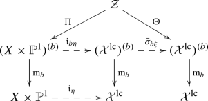  (259)

  For simplicity of notations, set ${\tilde{\phi }}_{t, b\xi }:=\Theta ^*\mathrm{m}_b^*{\bar{{{\mathcal {L}}}}}^\mathrm{lc}_t$ and ${\tilde{\psi }}:=\Pi ^*\mathrm{m}_b^* p_1^*(-K_X)$. Note that $\mathbf{D}^\mathrm{NA}$ and $\mathbf{L}^\mathrm{NA}$ are multiplicative under base change (see [38, Proposition 2.5.(3)]). Moreover, $\mathbf{L}^\mathrm{NA}$ is invariant under twisting: $\mathbf{L}^\mathrm{NA}({{\mathcal {X}}}^\mathrm{lc}_\xi , {{\mathcal {L}}}^\mathrm{lc}_{t, \xi })=\mathbf{L}({{\mathcal {X}}}^\mathrm{lc}, {{\mathcal {L}}}^\mathrm{lc}_{t})$ (by (114)). Then we can calculate

  $$\begin{aligned}&b V\cdot (\mathbf{D}^\mathrm{NA}({{\mathcal {X}}}^\mathrm{lc}_\xi , ({{\mathcal {L}}}^\mathrm{lc}_t)_\xi )-\epsilon \mathbf{J}^\mathrm{NA}({{\mathcal {X}}}^\mathrm{lc}_\xi , ({{\mathcal {L}}}^\mathrm{lc}_t)_\xi ))\\&\quad =V\cdot \left( (1-\epsilon )\mathbf{E}^\mathrm{NA}+\mathbf{L}^\mathrm{NA}-\epsilon {\varvec{\Lambda }}^\mathrm{NA}\right) ({{\mathcal {X}}}^\mathrm{lc}_{b\xi }, ({{\mathcal {L}}}^\mathrm{lc}_t)_{b\xi })\\&\quad = -\frac{1-\epsilon }{n+1}{\tilde{\phi }}_{t,b\xi }^{\cdot n+1}+1+(1+t) e_1 V-\epsilon {\tilde{\psi }}^{\cdot n}\cdot {\tilde{\phi }}_{t,b\xi }. \end{aligned}$$

  Taking derivative with respect to t, we get, for $0\le t\ll 1$:

  $$\begin{aligned}&b V\cdot \frac{d}{dt}\left[ \mathbf{D}^\mathrm{NA}({{\mathcal {X}}}^\mathrm{lc}_\xi , ({{\mathcal {L}}}^\mathrm{lc}_t)_\xi )-\epsilon \mathbf{J}^\mathrm{NA}({{\mathcal {X}}}^\mathrm{lc}_\xi , ({{\mathcal {L}}}^\mathrm{lc}_t)_\xi )\right] \\&\quad =-(1-\epsilon ){\tilde{\phi }}_{t,b\xi }^{\cdot n}\cdot \Theta ^*\mathrm{m}_b^*E+e_1 V-\epsilon {\tilde{\psi }}^{\cdot n}\cdot \Theta ^*\mathrm{m}_b^*E\\&\quad =-(1-\epsilon ){\tilde{\phi }}^{\cdot n}_{t, b\xi }\cdot \Theta ^*\mathrm{m}_b^*\sum _{j=1}^p(e_j-e_1)E_j-\epsilon {\tilde{\psi }}^{n-1}\\&\qquad \;\cdot \Theta ^*\mathrm{m}_b^*\sum _{j=1}^p (e_j-e_1)E_j\le 0. \end{aligned}$$

  The last inequality uses the relative nefness of ${\tilde{\phi }}_{t,b\xi }$ and ${\tilde{\psi }}$. After integration, we get, for any $0\le t\ll 1$:

  $$\begin{aligned}&d\cdot \left( \mathbf{D}^\mathrm{NA}({{\mathcal {X}}}_\xi , {{\mathcal {L}}}_\xi )-\epsilon \mathbf{J}^\mathrm{NA}({{\mathcal {X}}}_\xi , {{\mathcal {L}}}_\xi )\right) \nonumber \\&\quad =\mathbf{D}^\mathrm{NA}({{\mathcal {X}}}^\mathrm{lc}_\xi , ({{\mathcal {L}}}^\mathrm{lc}_0)_\xi )-\epsilon \mathbf{J}^\mathrm{NA}({{\mathcal {X}}}^\mathrm{lc}_\xi , ({{\mathcal {L}}}^\mathrm{lc}_0)_\xi )\nonumber \\&\quad \ge \mathbf{D}^\mathrm{NA}({{\mathcal {X}}}^\mathrm{lc}_\xi , ({{\mathcal {L}}}^\mathrm{lc}_t)_\xi )-\epsilon \mathbf{J}^\mathrm{NA}({{\mathcal {X}}}^\mathrm{lc}_\xi , ({{\mathcal {L}}}^\mathrm{lc}_t)_\xi ). \end{aligned}$$

  (260)

  We set ${{\mathcal {L}}}^\mathrm{lc}={{\mathcal {L}}}^\mathrm{lc}_t$ for some fixed $t\in {{\mathbb {Q}}}_{>0}$ sufficiently small.

• 2. Step 2: With the $({{\mathcal {X}}}^\mathrm{lc}, {{\mathcal {L}}}^\mathrm{lc})$ from the first step, we run a relative MMP with scaling to get a normal, ample test configuration $({{\mathcal {X}}}^\mathrm{ac}, {{\mathcal {L}}}^\mathrm{ac})$ for $(X, -K_X)$ such that $({{\mathcal {X}}}^\mathrm{ac}, {{\mathcal {X}}}^\mathrm{ac}_0)$ log canonical and $-K_{{{\mathcal {X}}}^\mathrm{ac}}\sim _{{{\mathbb {Q}}}}{{\mathcal {L}}}^\mathrm{ac}$ (the superscript “ac” stands for “anti-canonical”). More concretely, take $\ell \gg 1$ such that ${{\mathcal {H}}}^\mathrm{lc}={{\mathcal {L}}}^\mathrm{lc}-(\ell +1)^{-1}({{\mathcal {L}}}^\mathrm{lc}+K_{{{\mathcal {X}}}^\mathrm{lc}})$ is relatively ample. Set ${{\mathcal {X}}}^0={{\mathcal {X}}}^\mathrm{lc}$, ${{\mathcal {L}}}^0={{\mathcal {L}}}^\mathrm{lc}$, ${{\mathcal {L}}}^0={{\mathcal {H}}}^\mathrm{lc}$ and $\lambda _0=\ell _0+1$. Then $K_{{{\mathcal {X}}}^0}+\lambda _0{{\mathcal {H}}}^0=\ell {{\mathcal {L}}}^0$. We run a $K_{{{\mathcal {X}}}^0}$-MMP over ${{\mathbb {C}}}$ with scaling ${{\mathcal {H}}}^0$. Then we obtain a sequence of models:

  $$\begin{aligned} {{\mathcal {X}}}^0\dasharrow {{\mathcal {X}}}^1\dasharrow \cdots \dasharrow {{\mathcal {X}}}^k \end{aligned}$$

  and a sequence of critical values

  $$\begin{aligned} \lambda _{i+1}=\min \{\lambda ; K_{{{\mathcal {X}}}^i}+\lambda {{\mathcal {H}}}^i \text { is nef over } {{\mathbb {C}}}\} \end{aligned}$$

  with $\ell +1=\lambda _0\ge \lambda _1\ge \cdots \ge \lambda _k>\lambda _{k+1}=1$. For any $\lambda _i\ge \lambda \ge \lambda _{i+1}$, let ${{\mathcal {H}}}^i$ be the pushforward of ${{\mathcal {H}}}$ to ${{\mathcal {X}}}^i$ and set

  $$\begin{aligned} {{\mathcal {L}}}^i_\lambda =\frac{1}{\lambda -1}(K_{{{\mathcal {X}}}^i}+\lambda {{\mathcal {H}}}^i)=\frac{1}{\lambda -1}(K_{{{\mathcal {X}}}^i}+{{\mathcal {H}}}^i)+{{\mathcal {H}}}^i=:\frac{1}{\lambda -1}E+{{\mathcal {H}}}^i. \end{aligned}$$

  By the earlier discussion, $({{\mathcal {X}}}^i, {{\mathcal {L}}}^i)$ is indeed automatically $({{\mathbb {C}}}^*\times {\mathbb {G}})$-equivariant and E is a ${\mathbb {G}}$-invariant divisor supported on the central fibre ${{\mathcal {X}}}^i_0$. Write $E=\sum ^k_{j=1}e_j{{\mathcal {X}}}^i_{0,j}$ with $e_1\le e_2\le \cdots \le e_k$. Using similar diagram and notations as in Step 1, we can calculate

  $$\begin{aligned}&Vb\cdot \left( \mathbf{D}^\mathrm{NA}({{\mathcal {X}}}^i_\xi , {{\mathcal {L}}}^i_\xi )-\epsilon \mathbf{J}^\mathrm{NA}({{\mathcal {X}}}^i_\xi , {{\mathcal {L}}}^i_\xi )\right) \\&\quad =-(1-\epsilon )\frac{{\tilde{\phi }}_{\lambda ,b\xi }^{\cdot n+1}}{n+1}-\epsilon {\tilde{\psi }}^{\cdot n} \cdot {\tilde{\phi }}_{\lambda ,b\xi }+\frac{\lambda }{\lambda -1}e_1 V \end{aligned}$$

  whose derivative with respect to $\lambda$ is given by

  $$\begin{aligned} \frac{1}{(\lambda -1)^2}\sum _i \left( (1-\epsilon ){\tilde{\phi }}_{\lambda ,b\xi }^{\cdot n}+\epsilon {\tilde{\psi }}^{\cdot n}\right) \cdot (e_i-e_1) \Theta ^*\mathrm{m}_b^*E_i\ge 0. \end{aligned}$$

  (261)

  As in [39, 54], we verify easily that $\mathbf{F}^\mathrm{NA}({{\mathcal {X}}}^i_\xi , ({{\mathcal {L}}}^i_{\lambda _{i+1}})_\xi )=\mathbf{F}^\mathrm{NA}({{\mathcal {X}}}^{i+1}_{\xi }, ({{\mathcal {L}}}^{i+1}_{\lambda _{i+1}})_\xi )$ for $\mathbf{F}\in \{\mathbf{D}, \mathbf{J}\}$. Moreover by [54, Lemma 2], we know that $K_{{{\mathcal {X}}}^k}+{{\mathcal {L}}}^k_{\lambda _k}\sim _{{{\mathbb {Q}}}} 0$. Set ${{\mathcal {X}}}^\mathrm{ac}=\mathrm{Proj}\; R({{\mathcal {X}}}^k/{{\mathbb {C}}}, {{\mathcal {L}}}^k_{\lambda _k})$ and ${{\mathcal {L}}}^\mathrm{ac}=-K_{{{\mathcal {X}}}^\mathrm{ac}}$. After integrating (261) over each subinterval $[\lambda _{i+1}, \lambda _{i}]$ and summing up, we then get, for any $\xi \in N_{{\mathbb {Q}}}$:

  $$\begin{aligned}&\mathbf{D}^\mathrm{NA}({{\mathcal {X}}}^\mathrm{lc}_\xi , {{\mathcal {L}}}^\mathrm{lc}_\xi )-\epsilon \mathbf{J}^\mathrm{NA}({{\mathcal {X}}}^\mathrm{lc}_\xi , {{\mathcal {L}}}^\mathrm{lc}_\xi )\nonumber \\&\quad \ge \mathbf{D}^\mathrm{NA}({{\mathcal {X}}}^\mathrm{ac}_\xi , {{\mathcal {L}}}^\mathrm{ac}_\xi )-\epsilon \mathbf{J}^\mathrm{NA}({{\mathcal {X}}}^\mathrm{ac}_\xi , {{\mathcal {L}}}^\mathrm{ac}_\xi ). \end{aligned}$$

  (262)

• 3. Step 3: Combining the [54, Theorem 6] with the previous discussion on the equivariant MMP, we know that by a base change ${\tilde{{{\mathcal {X}}}}}^\mathrm{ac}={{\mathcal {X}}}^\mathrm{ac}\times _{{{\mathbb {C}}}, z^d}{{\mathbb {C}}}$ and running an appropriate $({{\mathbb {C}}}^*\times {\mathbb {G}})$-equivariant MMP, we can get a $({{\mathbb {C}}}^*\times {\mathbb {G}})$-equivariant diagram:

  

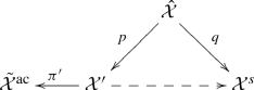  (263)

  which satisfies $A({{\mathcal {X}}}^s_0; {\tilde{{{\mathcal {X}}}}}^\mathrm{ac}, {\tilde{{{\mathcal {X}}}}}^\mathrm{ac}_0)=0$ and $\pi '$ exactly extracts the divisor ${{\mathcal {X}}}^s_0$ (here the superscript “s” stands for “special”). Then we have $\pi '^*K_{{\tilde{{{\mathcal {X}}}}}^\mathrm{ac}}=K_{{{\mathcal {X}}}'}$ and, with ${{\mathcal {L}}}^\mathrm{ac}=-K_{{{\mathcal {X}}}^\mathrm{ac}}$ (resp. ${\tilde{{{\mathcal {L}}}}}^\mathrm{ac}=-K_{{\tilde{{{\mathcal {X}}}}}^\mathrm{ac}}$) and ${{\mathcal {L}}}'=-K_{{{\mathcal {X}}}'}$,

  $$\begin{aligned}&d \cdot (\mathbf{D}^\mathrm{NA}({{\mathcal {X}}}^\mathrm{ac}_\xi , {{\mathcal {L}}}^\mathrm{ac}_\xi )-\epsilon \mathbf{J}^\mathrm{NA}({{\mathcal {X}}}^\mathrm{ac}_\xi , {{\mathcal {L}}}^\mathrm{ac}_\xi ))\\&\quad =\mathbf{D}^\mathrm{NA}({\tilde{{{\mathcal {X}}}}}^\mathrm{ac}_\xi , {\tilde{{{\mathcal {L}}}}}^\mathrm{ac}_\xi )-\epsilon \mathbf{J}^\mathrm{NA}({\tilde{{{\mathcal {X}}}}}^\mathrm{ac}_\xi , {\tilde{{{\mathcal {L}}}}}^\mathrm{ac}_\xi )\\&\quad =\mathbf{D}^\mathrm{NA}({{\mathcal {X}}}'_\xi , {{\mathcal {L}}}'_\xi )-\epsilon \mathbf{J}^\mathrm{NA}({{\mathcal {X}}}'_\xi , {{\mathcal {L}}}'_\xi ). \end{aligned}$$

  Set $E=p^*K_{{{\mathcal {X}}}'}-q^*K_{{{\mathcal {X}}}^s}=\sum _{i=1}^q e_i E_i$ with $e_1\le \cdots \le e_q$. Then $E\ge 0$ by the negativity lemma. Set $\hat{{\mathcal {L}}}_\lambda =-p^* K_{{{\mathcal {X}}}'/{{\mathbb {C}}}}+\lambda E$. Applying the diagram and notations similar to (259) in the first step to $({\hat{{{\mathcal {X}}}}}, {\hat{{{\mathcal {L}}}}}_\lambda )$, we get

  $$\begin{aligned}&V b\cdot \frac{d}{d\lambda }\left( \mathbf{D}^\mathrm{NA}({\hat{{{\mathcal {X}}}}}_\xi , ({\hat{{{\mathcal {L}}}}}_\lambda )_{\xi })-\epsilon \mathbf{J}^\mathrm{NA}({\hat{{{\mathcal {X}}}}}_\xi , ({\hat{{{\mathcal {L}}}}}_\lambda )_\xi )\right) \\&\quad = V \cdot \frac{d}{d\lambda }\left( (1-\epsilon )\frac{{\tilde{\phi }}_{\lambda , b\xi }^{\cdot n+1}}{n+1}-\epsilon {\tilde{\psi }}^{\cdot n}\cdot {\tilde{\phi }}_{\lambda , b\xi } +\lambda e_1\right) \\&\quad =-\sum _{i=1}^q \left( (1-\epsilon ){\tilde{\phi }}_{\lambda , b\xi }^{\cdot n}+\epsilon {\tilde{\psi }}^{\cdot n}\right) \cdot (e_i-e_1)E_i\le 0. \end{aligned}$$

  After integration we get

  $$\begin{aligned}&d \left( \mathbf{D}^\mathrm{NA}({{\mathcal {X}}}^\mathrm{ac}_\xi , {{\mathcal {L}}}^\mathrm{ac}_\xi )-\epsilon \mathbf{J}^\mathrm{NA}({{\mathcal {X}}}^\mathrm{ac}_\xi , {{\mathcal {L}}}^\mathrm{ac}_\xi )\right) \nonumber \\&\quad = \mathbf{D}^\mathrm{NA}({\hat{{{\mathcal {X}}}}}_\xi , ({\hat{{{\mathcal {L}}}}}_0)_\xi )-\epsilon \mathbf{J}^\mathrm{NA}({\hat{{{\mathcal {X}}}}}_\xi , ({\hat{{{\mathcal {L}}}}}_0)_\xi )\nonumber \\&\quad \ge \mathbf{D}^\mathrm{NA}({\hat{{{\mathcal {X}}}}}_\xi , ({\hat{{{\mathcal {L}}}}}_1)_\xi )-\epsilon \mathbf{J}^\mathrm{NA}({\hat{{{\mathcal {X}}}}}_\xi , ({\hat{{{\mathcal {L}}}}}_1)_\xi ) \nonumber \\&\quad =\mathbf{D}^\mathrm{NA}({{\mathcal {X}}}^s_\xi , {{\mathcal {L}}}^s_\xi )-\epsilon \mathbf{J}^\mathrm{NA}({{\mathcal {X}}}^s_\xi , {{\mathcal {L}}}^s_\xi ). \end{aligned}$$

  (264)

Finally, combining the inequalities (260), (262) and (264) from the above three steps, we get the conclusion. $\square$

Some properties of reductive groups

Jun Yu ²

Proposition B.1

Let G be a connected reductive complex Lie group and K be a maximal compact subgroup of G. Then we have $N_G(K)=C(G)\cdot K=C(G)_0\cdot K$ where $C(G)_0$ is the identity component of the center C(G) of G.

Proof

First we can decompose $G=C(G)_0\cdot G_1\cdot G_2\cdots G_s$ where $G_1, \dots , G_s$ are simple factors of G. By the connectedness assumption, this follows from the corresponding decomposition of the reductive Lie algebra ${\mathfrak {g}}=Lie(G)$ (see [48, Corollary 6.4, Theorem 6.24]). Write $K_i=K\cap G_i$, $K_0= K\cap C(G)_0$. Then $K=K_0\cdot K_1\cdots K_s$ and each $K_i$ is a maximal compact subgroup of $G_i$ ($1\le i\le s$). Clearly $C(G)_0\subset N_G(K)$.

Conversely, if $g=g_1\cdot g_2\cdots g_s$ (with $g_i\in G_i$) normalizes K, then $K=gKg^{-1}=K_0\cdot \prod _{i} g_i K_i g_i^{-1}$ which implies $g_i K_i g_i^{-1}=K\cap G_i=K_i$, i.e. each $g_i$ normalizes $K_i$. Hence it suffices to show that $N_{G_i}(K_i)=K_i$ for each $i (1\le i\le s)$. By this discussion, we may assume that G itself is simple. Write $H=N_G(K)$. Then H is a closed subgroup of G, and K is a normal subgroup of H.

Since G is assumed to be simple, the only Lie subalgebras of ${\mathfrak {g}}=\mathrm{Lie}(G)$ containing ${\mathfrak {k}}= \mathrm{Lie}(K)$ are ${\mathfrak {g}}$ and ${\mathfrak {k}}$. Thus ${\mathfrak {h}}=\mathrm{Lie}(H)={\mathfrak {g}}$ or ${\mathfrak {k}}$. When ${\mathfrak {h}}={\mathfrak {g}}$, then $H=G$ which is impossible.

When ${\mathfrak {h}}={\mathfrak {k}}$, H is also compact. Then for any $x\in H$, $\mathrm{Ad}(x)\in \mathrm{GL}({\mathfrak {g}})$ is elliptic (i.e. the eigenvalues of $\mathrm{Ad}(x)$ all have norm 1). On the other hand, we have the Cartan decomposition $G=K\exp ({\mathfrak {p}}_{0})$ where ${\mathfrak {p}}_{0}$ is the orthogonal complement of ${\mathfrak {k}}$ in ${\mathfrak {g}}$ with respect to the Killing form. Since for any $g\in \exp ({\mathfrak {p}}_{0})$, $\mathrm{Ad}(g)$ has positive real eigenvalues, $H\cap \exp ({\mathfrak {p}}_{0})=1$. Then

$$\begin{aligned} H=H\cap G=H\cap K\exp ({\mathfrak {p}}_{0})=K\cap (H\cap \exp ({\mathfrak {p}}_{0}))=K. \end{aligned}$$

$\square$

Proposition B.2

Let G be a connected complex reductive Lie group, and $K_1, K_2$ be two maximal compact subgroups. Assume that $K_1, K_2$ have a common maximal torus T. Set $T_{{\mathbb {C}}}=C_G(T)$ which is a maximal torus of G. Then the following hold true:

• (1) $K_2=t K_1 t^{-1}=: \mathrm{Ad}(t)K_1$ for some $t\in T_{{\mathbb {C}}}$.

• (2) If $K_2=\mathrm{Ad}(t) K_1$, then $K_1=K_2$ if and only if $t\in T$.

Proof

• (1) It is well-known that any two maximal compact subgroups of G are conjugate. Thus there exists $g\in G$ such that $K_2=\mathrm{Ad}(g)K_1$. Then $\mathrm{Ad}(g)T$ and T are maximal tori of $K_2$. Hence there exists $k_2\in K_2$ such that $\mathrm{Ad}(g)T= \mathrm{Ad}(k_2)T$. Set $g'=k_2^{-1}g$. Then

  $$\begin{aligned} \mathrm{Ad}(g')K_1=\mathrm{Ad}(k_2)\mathrm{Ad}(g)K_1=\mathrm{Ad}(k_2^{-1})K_2=K_2 \end{aligned}$$

  and

  $$\begin{aligned} \mathrm{Ad}(g')T=\mathrm{Ad}(k_2^{-1})\mathrm{Ad}(g)T=\mathrm{Ad}(k_2)^{-1}\mathrm{Ad}(k_2)T=T. \end{aligned}$$

  Thus $g'\in N_G(T)$. It is well-known that $T_{{\mathbb {C}}}:=C_G(T)$ is a maximal torus of G and

  $$\begin{aligned} N_G(T)=N_{K_2}(T)\cdot T_{{\mathbb {C}}}. \end{aligned}$$

  Write $g'=n\cdot t$ for $n\in N_{K_2}(T)$ and $t\in T_{{\mathbb {C}}}$. Then

  $$\begin{aligned} K_2=\mathrm{Ad}(n^{-1})K_2=\mathrm{Ad}(n^{-1})\mathrm{Ad}(g')K_1=\mathrm{Ad}(n^{-1}g')K_1=\mathrm{Ad}(t) K_1. \end{aligned}$$

• (2) Set ${\mathfrak {g}}=\mathrm{Lie}(G)$ and ${\mathfrak {t}}_{{\mathbb {C}}}=\mathrm{Lie}(T_{{\mathbb {C}}})$. Then one has a root space decomposition:

  $$\begin{aligned} {\mathfrak {g}}={\mathfrak {t}}_{{\mathbb {C}}}\bigoplus \left( \bigoplus _{\alpha \in \Delta }{\mathfrak {g}}_\alpha \right) , \end{aligned}$$

  where $\Delta =\Delta ({\mathfrak {g}}, {\mathfrak {t}}_{{\mathbb {C}}})$ are roots of ${\mathfrak {g}}$ with respect to ${\mathfrak {t}}_{{\mathbb {C}}}$ and ${\mathfrak {g}}_\alpha$ is the root space of $\alpha$. It is well-known that each ${\mathfrak {g}}_\alpha$ has dimension one. Chose $0\ne X_\alpha \in {\mathfrak {g}}_\alpha$ for any $\alpha \in \Delta$. Choose a positive system $\Delta ^+\subset \Delta$. It is well-known that

  $$\begin{aligned} {\mathfrak {k}}_1&{:=}&\mathrm{Lie}(K_1)\nonumber \\= & {} {\mathfrak {t}}\bigoplus \left( \bigoplus _{\alpha \in \Delta ^+}\big ({{\mathbb {R}}}(X_\alpha +a_\alpha X_{-\alpha })\oplus {{\mathbb {R}}}{\mathbf {i}}(X_\alpha +b_\alpha X_\alpha )\big )\right) \end{aligned}$$

  (265)

  for some constants $a_\alpha , b_\alpha \in {\mathbb {C}}^{\times }$ with $a_\alpha \ne b_\alpha$. Set ${\mathfrak {a}}$ to be the orthogonal complement of ${\mathfrak {t}}$ in ${\mathfrak {t}}_{{\mathbb {C}}}$ and $A=\mathrm{exp}({\mathfrak {a}})$. Then $T_{{\mathbb {C}}}=AT$. Assume $\mathrm{Ad}(t)K_1=K_1$. Clearly $\mathrm{Ad}(t_1)K_1=K_1$ for $t_1\in T\subset K_1$. So one may assume that $t=a\in A$. For any $\alpha \in \Delta ^+$, $\alpha (a)>0$. Then the Lie algebra of $\mathrm{Ad}(t)K_1=\mathrm{Ad}(a)K_1$ is equal to:

  $$\begin{aligned} {\mathfrak {t}}\bigoplus \left( \bigoplus _{\alpha \in \Delta ^+}\big ({{\mathbb {R}}}(X_\alpha +a_\alpha \alpha (a)^{-2}X_{-\alpha })\oplus {{\mathbb {R}}}{\mathbf {i}} (X_\alpha +b_\alpha \alpha (a)^{-2}X_{-\alpha })\big )\right) .\nonumber \\ \end{aligned}$$

  (266)

  For it to be equal to ${\mathfrak {k}}_1$, one must have $\alpha (a)^{-2}=1$ for all $\alpha \in \Delta ^+$. Then $a=1$.

$\square$

Proposition B.3

Let G be a connected complex reductive Lie group, and $K_1, K_2$ be two maximal compact subgroups. Assume that $K_1, K_2$ have a common compact subgroup K that in turn contains a maximal compact torus T of G. Then $K_2=t K_1 t^{-1}$ for some $t\in C(K_{{\mathbb {C}}})$ (the center of $K_{{\mathbb {C}}}$).

Proof

We use the same notations as in the proof of the last proposition. By Proposition B.2, there exists $t\in T_{{\mathbb {C}}}$ such that $K_2=t K_1 t^{-1}$. We just need to show that $t\in C(K_{{\mathbb {C}}})$. Similar to (265), we have the decomposition

$$\begin{aligned} {\mathfrak {k}}:=\mathrm{Lie}(K)={\mathfrak {t}}\bigoplus \left( \bigoplus _{\alpha \in \Delta '^+}\big ({{\mathbb {R}}}(X_\alpha +a_\alpha X_{-\alpha })\oplus {{\mathbb {R}}}{\mathbf {i}}(X_\alpha +b_\alpha X_\alpha )\big )\right) , \end{aligned}$$

where $\Delta '^+$ is a positive system for $\mathrm{Lie}(K_{{\mathbb {C}}})$ with respect to ${\mathfrak {t}}_{{\mathbb {C}}}$. Because $K_1\subseteq K$, ${\mathfrak {k}}$ embeds into ${\mathfrak {k}}_1$ via the inclusion $\Delta '^+\subseteq \Delta ^+$. By using the expression in (266), we see that the Lie algebra of $K_2=\mathrm{Ad}(t)K_1$ contains $\mathrm{Lie}(K)$ if and only if $\alpha (a)^{-2}=1$ for all $\alpha \in \Delta '^+$. This holds if and only if $t\in C(K_{{\mathbb {C}}})$. $\square$

References

Ahag, P., Cegrell, U., Kołdziej, S., Pham, H.H., Zeriahi, A.: Partial pluricomplex energy and integrability exponents of plurisubharmonic functions. Adv. Math. 222, 2036–2058 (2009)
Akhiezer, D.N.: Lie Group Actions in Complex Analysis, No. E27 in Aspects of Mathematics. Friedr Vieweg & Sohn, Braunschweig (1995)
Altmann, K., Hausen, J., Süss, H.: Gluing affine torus actions via divisorial fans. Transform. Groups 13(2), 215–242 (2008)
Andreatta, M.: Actions of linear algebraic groups on projective manifolds and minimal model program. Osaka J. Math. 38, 151–166 (2001)
Berman, R.: K-stability of \({ Q}\)-Fano varieties admitting Kähler–Einstein metrics. Invent. Math. 203(3), 973–1025 (2015)
Berman, R., Berndtsson, R.: Convexity of the K-energy on the space of Kähler metrics. J. Am. Math. Soc. 30, 1165–1196 (2017)
Berman, R., Boucksom, S., Eyssidieux, P., Guedj, V., Zeriahi, A.: Kähler–Einstein metrics and the Kähler–Ricci flow on log Fano varieties. J. Reine Angew. Math. 751, 27–89 (2019)
Boucksom, S., Favre, C., Jonsson, M.: Singular semipositive metrics in non-Archimedean geometry. J. Algebraic Geom. 25, 77–139 (2016)
Berman, R., Boucksom, S., Jonsson, M.: A variational approach to the Yau–Tian–Donaldson conjecture. arXiv:1509.04561v1
Berman, R., Boucksom, S., Jonsson, M.: A variational approach to the Yau–Tian–Donaldson conjecture. J. Am. Math. Soc. arXiv:1509.04561v3
Birkar, C., Cascini, P., Hacon, C.D., McKernan, J.: Existence of minimal models for varieties of log general type. J. Am. Math. Soc. 23, 405–468 (2010)
Berman, R., Darvas, T., Lu, C.H.: Convexity of the extended K-energy and the large time behaviour of the weak Calabi flow. Geom. Topol. 21, 2945–2988 (2017)
Berndtsson, B.: A Brunn–Minkowski type inequality for Fano manifolds and some uniqueness theorems in Kähler geometry. Invent. Math. 200(1), 149–200 (2015)
Blum, H., Jonsson, M.: Thresholds, valuations and K-stability. Adv. Math. 365, 107062 (2020). arXiv:1706.04548
Boucksom, S., Chen, H.: Okounkov bodies of filtered linear series. Compos. Math. 147, 1205–1229 (2011)
Boucksom, S., Eyssidieux, P., Guedj, V., Zeriahi, A.: Monge–Ampère equations in big cohomology classes. Acta Math. 205, 199–262 (2010)
Boucksom, S., de Fernex, T., Favre, C., Urbinati, S.: Valuation spaces and multiplier ideals on singular varieties. In: Recent Advances in Algebraic Geometry, London Math. Soc. Lecture Note Ser., vol. 417, pp. 29–51. Cambridge Univ. Press, Cambridge (2015)
Boucksom, S., Favre, C., Jonsson, M.: Valuations and plurisubharmonic singularities. Publ. RIMS 44, 449–494 (2008)
Boucksom, S., Hisamoto, T., Jonsson, M.: Uniform K-stability, Duistermaat–Heckman measures and singularities of pairs. Ann. Inst. Fourier (Grenoble) 67, 87–139 (2017). arXiv:1504.06568
Boucksom, S., Hisamoto, T., Jonsson, M.: Uniform K-stability and asymptotics of energy functionals in Kähler geometry. J. Eur. Math. Soc. (JEMS) 21(9), 2905–2944 (2019)
Boucksom, S., Jonsson, M.: Global pluripotential theory over a trivially valued field. arXiv:1801.08229v2
Boucksom, S., Jonsson, M.: A non-Archimedean approach to K-stability. arXiv:1805.11160v1
Brion, M.: Sur l’image de l’application moment. Séminaire d’Algèbre Paul Dubreil et Marie-Paul Malliavin Lect. Notes Math., vol. 1296. Springer (1987)
Brion, M., Samuel, P., Uma, V.: Lectures on the Structure of Algebraic Groups and Geometric Applications, CMI Lecture Series in Mathematics, vol. 1. Hindustan Book Agency, New Delhi; Chennai Mathematical Institute (CMI), Chennai (2013)
Chen, X.X., Donaldson, S.K., Sun, S.: Kähler–Einstein metrics on Fano manifolds, I–III. J. Am. Math. Soc. 28, 183–197, 199–234, 235–278 (2015)
Coman, D., Guedj, V., Zeriahi, A.: Extension of plurisubharmonic functions with growth control. J. Reine Angew. Math. 676, 33–49 (2013)
Datar, V., Székelyhidi, G.: Kähler–Einstein metrics along the smooth continuity method. Geom. Funct. Anal. 26(4), 975–1010 (2016)
Darvas, T.: The Mabuchi geometry of finite energy classes. Adv. Math. 285, 182–219 (2015)
Darvas, T.: Metric geometry of normal Kähler spaces, energy properness, and existence of canonical metrics. Int. Math. Res. Not. (IMRN) 17, 6752–6777 (2017)
Darvas, T., Rubinstein, Y.: Tian’s properness conjectures and Finsler geometry of the space of Kähler metrics. J. Am. Math. Soc. 30, 347–387 (2017)
Demailly, J.-P.: Regularization of closed positive currents and intersection theory. J. Algebraic Geom. 1, 361–409 (1992)
Di Nezza, E., Guedj, V.: Geometry and topology of the space of Kähler metrics. Compos. Math. 154, 1593–1632 (2018)
Dervan, R.: Uniform stability of twisted constant scalar curvature Kähler metrics. Int. Math. Res. Not. no. 15, 4728–4783 (2016)
Ding, W.Y.: Remarks on the existence problem of positive Kähler–Einstein metrics. Math. Ann. 282, 463–471 (1988)
Donaldson, S.: Scalar curvature and stability of toric varieties. J. Differ. Geom. 62(2), 289–349 (2002)
Donaldson, S.: Lower bounds of the Calabi functional. J. Differ. Geom. 70, 453–472 (2005)
Fornaess, J.E., Narasimhan, R.: The Levi problem on complex spaces with singularities. Math. Ann. 248, 47–72 (1980)
Fujita, K.: Optimal bounds for the volumes of Kähler–Einstein Fano manifolds. Am. J. Math. 140(2), 391–414 (2018)
Fujita, K.: A valuative criterion for uniform K-stability of \({\mathbb{Q}}\)-Fano varieties. J. Reine Angew. Math. 751, 309–338 (2019)
Fujita, K.: Uniform K-stability and plt blowups. Kyoto J. Math. 59(2), 399–418 (2019)
Guedj, V., Zeriahi, A.: Degenerate complex Monge–Ampère equations, book, 470 pp. EMS Tracts in Mathematics (2017)
Golota, A.: Delta-invariants for Fano varieties with large automorphism groups. arXiv:1907.06261
Guedj, V., Zeriahi, A.: The weighted Monge–Ampère energy of quasiplurisubharmonic functions. J. Funct. Anal. 250(2), 442–482 (2007)
Hisamoto, T.: Orthogonal projection of a test configuration to vector fields. arXiv:1610.07158
Hisamoto, T.: Stability and coercivity for toric polarizations. arXiv:1610.07998
Hisamoto, T.: Mabuchi’s soliton metric and relative D-stability. arXiv:1905.05948
Jonsson, M., Mustaţă, M.: Valuations and asymptotic invariants for sequences of ideals. Ann. Inst. Fourier 62(6), 2145–2209 (2012)
Kirillov, A., Jr.: An Introduction to Lie Groups and Lie Algebras, Cambridge Studies in Advanced Mathematics, vol. 113. Cambridge University Press, Cambridge (2008)
Kollár, J.: Lectures on Resolution of Singularities, Annals of Mathematics Studies, vol. 166. Princeton University Press, Princeton, NJ (2007)
Kollár, J., Mori, S.: Birational Geometry of Algebraic Varieties. Cambridge Tracts in Mathematics, vol. 134. Cambridge University Press, Cambridge (1998)
Li, C.: Minimizing normalized volume of valuations. Math. Z. 289(1–2), 491–513 (2018)
Li, C.: K-semistability is equivariant volume minimization. Duke Math. J. 166(16), 3147–3218 (2017)
Li, C.: Geodesic rays and stability in the cscK problem. arXiv:2001.01366
Li, C., Xu, C.: Special test configurations and K-stability of Fano varieties. Ann. Math. (2) 180(1), 197–232 (2014)
Li, Y., Tian, G., Zhu, X.: Uniform K-stability modulo a group for stable pairs (in preparation)
Li, C., Tian, G., Wang, F.: On Yau–Tian–Donaldson conjecture for singular Fano varieties. arXiv:1711.09530
Li, C., Tian, G., Wang, F.: The uniform version of Yau–Tian–Donaldson conjecture for singular Fano varieties. arXiv:1903.01215
Liu, Y., Xu, C., Zhuang, Z.: Finite generation for valuations computing stability thresholds and applications to K-stability. arXiv:2102.09405
Milne, J.: Algebraic Groups. The Theory of Group Schemes of Finite Type Over a Field. Cambridge Studies in Advanced Mathematics, vol. 170. Cambridge University Press, Cambridge (2017)
Odaka, Y.: The GIT stability of polarized varieties via discrepancy. Ann. Math. 177, 645–661 (2013)
Okounkov, A.: Brunn–Minkowski inequality for multiplicities. Invent. Math. 125, 405–411 (1996)
Pasquier, B.: Birational geometry of G-varieties, online lecture notes (2017)
Phong, D.H., Ross, J., Sturm, J.: Deligne pairings and the Knudsen–Mumford expansion. J. Differ. Geom. 78, 475–496 (2008)
Süß, H.: Kähler–Einstein metrics on symmetric Fano T-varieties. Adv. Math. 246, 100–113 (2013)
Székelyhidi, G.: Filtrations and test configurations, with an appendix by S. Boucksom. Math. Ann. 362(1–2), 451–484 (2015)
Tian, G.: Canonical Metrics in Kähler Geometry. Lectures in Mathematics ETH Zürich. Birkhäuser, Basel (2000)
Tian, G.: Kähler–Einstein metrics with positive scalar curvature. Invent. Math. 137, 1–37 (1997)
Tian, G., et al.: Existence of Einstein metrics on Fano manifolds. In: Dai, X.-Z. (ed.) Metric and Differential Geometry, pp. 119–159. Springer, Berlin (2012)
Tian, G.: K-stability and Kähler–Einstein metrics. Commun. Pure Appl. Math. 68(7), 1085–1156 (2015)
Witt Nyström, D.: Test configuration and Okounkov bodies. Compos. Math. 148(6), 1736–1756 (2012)
Zhu, Z.: A note on equivariant K-stability. arXiv:1907.07655
Acknowledgements
The author is partially supported by NSF (Grant No. DMS-1810867) and an Alfred P. Sloan research fellowship. I would like to thank Gang Tian for constant support and his interest in this work, and thank Xiaowei Wang for helpful discussions on related topics, Feng Wang, Xiaohua Zhu and Chenyang Xu for helpful comments, Sébastien Boucksom for his interest in our work, and Tomoyuki Hisamoto for communications concerning Remark 5.10. I would like to thank Yuchen Liu for comments and clarifications, which motivate me to write down the results for more general reductive subgroups, and thank Jiyuan Han and Kuang-Ru Wu for attending my lectures about this work patiently and give valuable feedback which allows me to improve the presentation. I am particularly grateful to Jun Yu for answering my questions in the appendix concerning reductive groups. Some parts of this paper were written during the author’s visit to BICMR at Peking University, School of Mathematical Sciences at Capital Normal University and Shanghai Center for Mathematical Sciences at Fudan University. I would like to thank these institutes for providing wonderful environment of research. In particular, I would like to thank Gang Tian, Zhenlei Zhang and Peng Wu for their hospitality. I would also like to thank anonymous referees for their careful reading and providing very helpful comments for improving the paper.
Author information
Authors and Affiliations
Corresponding author
Additional information
Publisher's Note
Springer Nature remains neutral with regard to jurisdictional claims in published maps and institutional affiliations.