Associative Submanifolds in Joyce’s Generalised Kummer Constructions

Abstract

This article constructs examples of associative submanifolds in $G_2$–manifolds obtained by resolving $G_2$–orbifolds using Joyce’s generalised Kummer construction. As the $G_2$–manifolds approach the $G_2$–orbifolds, the volume of the associative submanifolds tends to zero. This partially verifies a prediction due to Halverson and Morrison.

1 Introduction

The Teichmüller space

$$\begin{aligned} \mathscr {T}(Y) :=\left\{ \phi \in \Omega ^3(Y): \phi ~\text{ is } \text{ a } \text{ torsion-free }\ G_2\text{--structure } \right\} /{{\,\text {Diff}\,}}_0(Y) \end{aligned}$$

of torsion-free $G_2$–structures on a closed 7–manifold Y is a smooth manifold of dimension $b^3(Y)$ [Joy96a, Theorem C]. The $G_2$ period map $\Pi :\mathscr {T}\rightarrow \textrm{H}_{\textrm{dR}}^3(Y) \oplus \textrm{H}_{\textrm{dR}}^4(Y)$ defined by

$$\begin{aligned} \Pi \left( {\phi \cdot {{\,\textrm{Diff}\,}}_0(Y)}\right) :=([\phi ],[\psi ]) \quad \text {with}\quad \psi :=*_\phi \phi \end{aligned}$$

is a Lagrangian immersion [Joy96b, Lemma 1.1.3].¹ It is constrained by the following inequalities [Joy96b, Lemma 1.1.2]; [HL82, §IV.2.A and §IV.2.B]:

• (1) ${\displaystyle \int _Y \alpha \wedge \alpha \wedge \phi < 0}$   for every non-zero $[\alpha ] \in \textrm{H}_{\textrm{dR}}^2(Y)$ if $\pi _1(Y)$ is finite.

• (2) ${\displaystyle \int _Y p_1(V) \wedge \phi = -\tfrac{1}{4\pi ^2} \textrm{YM}(A) < 0}$   for every vector bundle V which admits a non-flat $G_2$–instanton A; in particular, for $V = TY$ unless Y is covered by $T^7$. Here $p_1(V)$ denotes the $1^{\text {st}}$ Pontryagin class of V [MS74, §15], and $\textrm{YM}(A) :=\frac{1}{2} \int _Y |F_A|^2$ is the Yang–Mills energy.

• (3) ${\displaystyle \int _P \phi = \textrm{vol}(P) > 0}$   for every associative submanifold $P \looparrowright Y$.

• (4) ${\displaystyle \int _Q \psi = \textrm{vol}(Q) > 0}$   for every coassociative submanifold $Q \looparrowright Y$.

These should be compared with the inequalities cutting out the Kähler cone of a Calabi–Yau 3–fold; see Wilson [Wil92].

By analogy with Calabi–Yau 3–folds, Halverson and Morrison [HM16, §3] suggest that the above inequalities completely characterise the ideal boundary of $\mathscr {T}(Y)$. Of course, making this precise is complicated by the fact that the notions of $G_2$–instanton and (co)associative submanifold depend on the $G_2$–structure $\phi$. The situation would be improved if there were invariants whose non-vanishing guaranteed the existence of $G_2$–instantons and (co)associative submanifolds as suggested by Donaldson and Thomas [DT98, §3]. However, their construction is fraught with enormous difficulty [DS11, Joy18, Hay17, Wal17, DW19].

A more down to earth problem is to exhibit concrete examples of degenerating families of $G_2$–manifolds which admit $G_2$–instantons whose Yang–Mills energies tend to zero [Wal13] or which admit (co)associative submanifolds whose volumes tend to zero. The purpose of this article is to present examples of the latter in $G_2$–manifolds arising from Joyce’s generalised Kummer construction. Although these examples had been anticipated (e.g. by Halverson and Morrison [HM16, §6.2]), their rigorous construction has only recently become possible due to the work of Platt [Pla22].

Remark 1.1

Of course, there are already numerous examples of closed associative submanifolds in the literature.

• (1) Joyce [[Joy96b, §4.2];  [Joy00, §12.6]] has constructed (co)associative submanifolds in generalised Kummer constructions as fixed-point sets of involutions.

• (2) Corti, Haskins, Nordström, and Pacini [CHNP15, §5.5 and §7.2.2] have constructed associative submanifolds in twisted connected sums using rigid holomorphic curves and special Lagrangians in asymptotically cylindrical Calabi–Yau 3–folds.

• (3) In the physics literature, Braun, Del Zotto, Halverson, Larfors, Morrison, and Schäfer Nameki [BDHLMS18, §4.4] have proposed a construction of infinitely many associative submanifolds in certain twisted connected sums. An important ingredient in the proof of this conjecture will be the gluing theorem for associative submanifolds in twisted connected sums proved by Bera [Ber22]—analogous to [SW15]. Building on [BDHLMS18], Acharya, Braun, Svanes, and Valandro [ABSV19, §2.2 and §4.2] have constructed infinitely many associative submanifolds in certain $G_2$–orbifolds (without using any analytic methods).

• (4) Lotay [Lot12], Kawai [Kaw15], Ball and Madnick [BM20] have produced a wealth of examples of associative submanifolds in $S^7$, the squashed $S^7$, and the Berger space with their nearly parallel $G_2$–structures.

The novelty of the examples discussed in the present article is that their volumes tend to zero as the ambient $G_2$–manifolds degenerate.

2 Joyce’s Generalised Kummer Construction

The generalised Kummer construction is a method, developed by Joyce [Joy96a, Joy96b], to produce $G_2$–manifolds by desingularising certain closed flat $G_2$–orbifolds $(Y_0,\phi _0)$. Besides a rather delicate singular perturbation theory it relies on the fact that the hyperkähler 4–orbifolds $\textbf{H}/\Gamma$, obtained as quotients of the quaternions $\textbf{H}$ by a finite subgroup $\Gamma < \textrm{Sp}(1)$, can be desingularised by hyperkähler 4–manifolds. The following model spaces feature prominently throughout this article.

Example 2.1

(model spaces) Let X be a hyperkähler 4–orbifold with hyperkähler form

$$\begin{aligned} {\varvec{\omega {}}}\in ({\text {Im}}\textbf{H})^* \otimes \Omega ^2(X). \end{aligned}$$

Denote by $\textrm{vol}\in \Omega ^3({\text {Im}}\textbf{H})$ and $\textbf{1}\in \Omega ^1({\text {Im}}\textbf{H}) \otimes {\text {Im}}\textbf{H}$ the volume form and the tautological 1–form respectively.

• (1) The 3–form

  $$\begin{aligned} \textrm{vol}- \left\langle \textbf{1}\wedge {\varvec{\omega {}}}\right\rangle \in \Omega ^3({\text {Im}}\textbf{H}\times X) \end{aligned}$$

  (2.2)

  defines a torsion-free $G_2$–structure on ${\text {Im}}\textbf{H}\times X$. Here $\left\langle \cdot \wedge \cdot \right\rangle$ is induced by the wedge product on forms and the duality pairing between ${\text {Im}}\textbf{H}$ and $({\text {Im}}\textbf{H})^*$. The corresponding Riemannian metric and the cross-product on ${\text {Im}}\textbf{H}\times X$ recover the Riemannian metric and the hypercomplex structure ${\textbf{I}}\in ({\text {Im}}\textbf{H})^* \otimes \Gamma ({{\,\textrm{End}\,}}(TX))$ on X.

• (2) Let $G < \textrm{SO}({\text {Im}}\textbf{H}) < imes {\text {Im}}\textbf{H}$ be a Bieberbach group; that is: discrete, cocompact, and torsion-free. Let $\rho :G \rightarrow {{\,\textrm{Isom}\,}}(X)$ be a homomorphism. Suppose that ${\varvec{\omega {}}}$ is G–invariant; that is: for every $(R,t) \in G$

  $$\begin{aligned} \big ({R^* \otimes \rho (R,t)^*}\big ) {\varvec{\omega {}}}= {\varvec{\omega {}}}. \end{aligned}$$

  Set

  $$\begin{aligned} Y :=({\text {Im}}\textbf{H}\times X)/G. \end{aligned}$$

  The $G_2$–structure (2.2) descends to a $G_2$–structure

  $$\begin{aligned} \phi \in \Omega ^3(Y). \end{aligned}$$

  The canonical projection $p :Y \rightarrow B :={\text {Im}}\textbf{H}/G$ is a flat fibre bundle whose fibres are coassociative submanifolds diffeomorphic to X; cf. [Bar19, §3.4]. $\spadesuit$

Remark 2.3

(Classification of Bieberbach groups) If $G < \textrm{SO}({\text {Im}}\textbf{H}) < imes {\text {Im}}\textbf{H}$ is a Bieberbach group, then $\Lambda :=G \cap {\text {Im}}\textbf{H}< {\text {Im}}\textbf{H}$ is a lattice of full rank and $H :=G/\Lambda < \textrm{SO}(\Lambda ) \times ({\text {Im}}\textbf{H}/\Lambda )$ is isomorphic to either $\textbf{1}$, $C_2$, $C_3$, $C_4$, $C_6$, or $C_2^2$; cf. [HW35, CR03, Szc12, §3.3]. More precisely, G is among the following:

($\textbf{1}$):

$\Lambda$ is arbitrary and $G = \Lambda$.

($C_2$):

$\Lambda = \left\langle \lambda _1,\lambda _2,\lambda _3\right\rangle$ with

$$\begin{aligned} \left\langle \lambda _1,\lambda _2\right\rangle = \left\langle \lambda _1,\lambda _3\right\rangle = 0. \end{aligned}$$

G is generated by $\Lambda$ and $(R_2,\frac{1}{2}\lambda _1)$ with $R_2 \in \textrm{SO}(\Lambda )$ as in (2.5).

($C_3$):

$\Lambda = \left\langle \lambda _1,\lambda _2,\lambda _3\right\rangle$ with

$$\begin{aligned} \left\langle \lambda _1,\lambda _2\right\rangle = \left\langle \lambda _1,\lambda _3\right\rangle = 0 \quad \text {and}\quad |\lambda _2|^2 = |\lambda _3|^2 = -2\left\langle \lambda _2,\lambda _3\right\rangle . \end{aligned}$$

(2.4)

G is generated by $\Lambda$ and $(R_3,\frac{1}{3}\lambda _1)$ with $R_3 \in \textrm{SO}(\Lambda )$ as in (2.5).

($C_4$):

$\Lambda = \left\langle \lambda _1,\lambda _2,\lambda _3\right\rangle$ with

$$\begin{aligned} \left\langle \lambda _1,\lambda _2\right\rangle = \left\langle \lambda _2,\lambda _3\right\rangle = \left\langle \lambda _3,\lambda _1\right\rangle = 0 \quad \text {and}\quad |\lambda _2|^2 = |\lambda _3|^2. \end{aligned}$$

G is generated by $\Lambda$ and $(R_4,\frac{1}{4}\lambda _1)$ with $R_4 \in \textrm{SO}(\Lambda )$ as in (2.5).

($C_6$):

$\Lambda = \left\langle \lambda _1,\lambda _2,\lambda _3\right\rangle$ with (2.4). G is generated by $\Lambda$ and $(R_6,\frac{1}{6}\lambda _1)$ with $R_6 \in \textrm{SO}(\Lambda )$ as in (2.5).

($C_2^2$):

$\Lambda = \left\langle \lambda _1,\lambda _2,\lambda _3\right\rangle$ with

$$\begin{aligned} \left\langle \lambda _1,\lambda _2\right\rangle = \left\langle \lambda _2,\lambda _3\right\rangle = \left\langle \lambda _3,\lambda _1\right\rangle = 0. \end{aligned}$$

G is generated by $\Lambda$, $(R_+,\frac{1}{2}(\lambda _1+\lambda _2))$, and $(R_-,\frac{1}{2}(\lambda _2+\lambda _3))$ with $R_\pm \in \textrm{SO}(\Lambda )$ as in (2.5).

Here $R_2,R_3,R_4,R_6,R_\pm \in {{\,\textrm{GL}\,}}_3(\textbf{Z})$ are defined by

$$\begin{aligned} \begin{aligned} R_2 :=\begin{pmatrix} 1 &{} 0 &{} 0 \\ 0 &{} -1 &{} 0\\ 0 &{} 0 &{} -1 \end{pmatrix}, \quad R_3 :=\begin{pmatrix} 1 &{} 0 &{} 0\\ 0 &{} -1 &{} 1 \\ 0 &{} -1 &{} 0 \end{pmatrix}, \quad R_4 :=\begin{pmatrix} 1 &{} 0 &{} 0\\ 0 &{} 0 &{} 1 \\ 0 &{} -1 &{} 0 \end{pmatrix}, \\ R_6 :=\begin{pmatrix} 1 &{} 0 &{} 0\\ 0 &{} 1 &{} -1 \\ 0 &{} 1 &{} 0 \end{pmatrix}, \quad \text {and}\quad R_\pm :=\begin{pmatrix} \pm 1 &{} 0 &{} 0 \\ 0 &{} \mp 1 &{} 0 \\ 0 &{} 0 &{} -1 \end{pmatrix}. \end{aligned} \end{aligned}$$

(2.5)

${{\,\textrm{GL}\,}}_3(\textbf{Z})$ is identified with ${{\,\textrm{GL}\,}}(\Lambda )$ by the choice of generators of $\Lambda$. $\clubsuit$

The version of the generalised Kummer construction considered in this article desingularises closed flat $G_2$–orbifolds $(Y_0,\phi _0)$ whose singularities are modelled on Example 2.1 with $X :=\textbf{H}/\Gamma$ for finite $\Gamma < \textrm{Sp}(1)$. This requires a choice of the following data; cf. [Joy00, §11.4.1].

Definition 2.6

Let $(Y_0,\phi _0)$ be a flat $G_2$–orbifold. Denote the connected components of the singular set of $Y_0$ by $S_\alpha$ ($\alpha \in A$). Resolution data ${\mathfrak R}= (\Gamma _\alpha ,G_\alpha ,\rho _\alpha ;R_\alpha ,\jmath _\alpha ;\hat{X}_\alpha ,\hat{\varvec{\omega {}}}_\alpha ,\hat{\rho }_\alpha ,\tau _\alpha )_{\alpha \in A}$ for $(Y_0,\phi _0)$ consist of the following for every $\alpha \in A$:

• (1) A finite subgroup $\Gamma _\alpha< \textrm{Sp}(1) < \textrm{SO}(\textbf{H})$, a Bieberbach group $G_\alpha < \textrm{SO}({\text {Im}}\textbf{H}) < imes {\text {Im}}\textbf{H}$, and a homomorphism $\rho _\alpha :G_\alpha \rightarrow N_{\textrm{SO}(\textbf{H})}(\Gamma _\alpha ) \hookrightarrow {{\,\textrm{Isom}\,}}(\textbf{H}/\Gamma _\alpha )$ as in Example 2.1 (2) with $X :=\textbf{H}/\Gamma _\alpha$ and its canonical hyperkähler form ${\varvec{\omega {}}}$. Here $N_G(H)$ denotes the normaliser of $H < G$. Denote by $(Y_\alpha ,\phi _\alpha )$ the model space associated with $\textbf{H}/\Gamma _\alpha$, ${\varvec{\omega {}}}$, $G_\alpha$, and $\rho _\alpha$.

• (2) $R_\alpha >0$ defining the open set

  $$\begin{aligned} U_\alpha :=\big ({{\text {Im}}\textbf{H}\times \left( {B_{2R_\alpha }(0)/\Gamma _\alpha }\right) }\big )/G_\alpha \subset Y_\alpha , \end{aligned}$$

  and an open embedding $\jmath _\alpha :U_\alpha \hookrightarrow Y_0$ satisfying $S_\alpha \subset {{\,\textrm{im}\,}}\jmath _\alpha$ and

  $$\begin{aligned} \jmath _\alpha ^*\phi _0 = \phi _{\alpha }. \end{aligned}$$

• (3) A hyperkähler 4–manifold $\hat{X}_\alpha$ with hyperkähler form $\hat{\varvec{\omega {}}}_\alpha \in ({\text {Im}}\textbf{H})^* \otimes \Omega ^2(\hat{X}_\alpha )$, a homomorphism $\hat{\rho }_\alpha :G_\alpha \rightarrow {{\,\textrm{Diff}\,}}(\hat{X}_\alpha )$ with respect to which $\hat{\varvec{\omega {}}}_\alpha$ is $G_\alpha$–invariant (in the sense of Example 2.1 (2)), a compact subset $K_\alpha \subset \hat{X}_\alpha$, and a $G_\alpha$–equivariant open embedding $\tau _\alpha :\hat{X}_\alpha {\setminus } K_\alpha \hookrightarrow \textbf{H}/\Gamma _\alpha$ with $\left( {\textbf{H}{\setminus } B_{R_\alpha }(0)}\right) /\Gamma \subset {{\,\textrm{im}\,}}\tau _\alpha$ and

  $$\begin{aligned} |\nabla ^k\left( {\tau _*\hat{\varvec{\omega {}}}_\alpha -{\varvec{\omega {}}}}\right) | = O\left( {r^{-4-k}}\right) \end{aligned}$$

  (2.7)

  for every $k \in {\textbf{N}}_0$. $\bullet$

Remark 2.8

(ADE classification of finite subgroups of $\textrm{Sp}(1)$) Klein [Kle93] classified the (non-trivial) finite subgroups $\Gamma < \textrm{Sp}(1)$. They obey an ADE classification. $\Gamma$ is isomorphic to either:

($A_k$):

a cyclic group $C_{k+1}$,

$(D_k)$:

a dicyclic group $\textrm{Dic}_{k-2}$,

($E_6$):

the binary tetrahedral group 2T,

($E_7$):

the binary octahedral group 2O, or

($E_8$):

the binary icosahedral group 2I. $\clubsuit$

Remark 2.9

Whether or not the data in Definition 2.6 (1) and (2) exists is a property of a neighborhood of the singular set of $Y_0$. If it does exist, then it is essentially unique. The data in Definition (2.6) (3) involves a choice. $\clubsuit$

Remark 2.10

There are many examples of closed flat $G_2$–orbifolds admitting resolution data in the above sense; see [Joy96b, §3];[Joy00, §12];[Bar06, §3];[Rei17, §5.3.4 and §5.3.5]. They arise from certain crystallographic groups $G < G_2 < imes \textbf{R}^7$. It would be interesting to classify these (possibly computer-aided) to grasp the full scope of Joyce’s generalised Kummer construction. Partial results have been obtained by Barrett [Bar06, §3.2], and Reidegeld [Rei17, Theorem 5.3.1] proved that the only possibilities for $\Gamma _\alpha$ in Definition 2.6 (1) are $C_2$, $C_3$, $C_4$, $C_6$, $\textrm{Dic}_2$, $\textrm{Dic}_3$, and 2T. $\clubsuit$

Remark 2.11

(scaling resolution data) For every $(t_\alpha ) \in (0,1]^A$ the data $\hat{\varvec{\omega {}}}_\alpha$ and $\tau _\alpha$ in Definition 2.6 (3) can be replaced with $t_\alpha ^2\hat{\varvec{\omega {}}}_\alpha$ and $t_\alpha \tau _\alpha$. $\clubsuit$

The following two lengthy remarks help to find resolution data ${\mathfrak R}$ with certain properties.

Remark 2.12

(Gibbons–Hawking construction of $A_k$ ALE spaces) Let $k \in {\textbf{N}}$. Consider the subgroup $C_k \hookrightarrow \textrm{Sp}(1)$ generated by right multiplication with $e^{2\pi i/k}$. (Of course, i can be replaced by $\hat{\xi }\in S^2 \subset {\text {Im}}\textbf{H}$ throughout.) The $A_k$ ALE hyperkähler 4–manifolds used to resolve $\textbf{H}/C_k$ can be understood concretely using the Gibbons–Hawking construction [GH78, GRG97, §3.5].

• (1) Let

  $$\begin{aligned} \varvec{\zeta } \in \Delta := \mathrm{{{\,\textrm{Sym}\,}}}_0^k (\mathrm{{\text {Im}}} \mathbf{\textbf{H}}) := \left\{ [\zeta _1,\ldots ,\zeta _k] \in (\mathrm{{\text {Im}}} \mathbf{\textbf{H}}^k)/S_k: \zeta _1+\cdots +\zeta _k = 0 \right\} . \end{aligned}$$

  Set $Z :=\left\{ \zeta _1,\ldots ,\zeta _k \right\}$ and $B :={\text {Im}}\textbf{H}{\setminus } Z$. The function $V_{\varvec{\zeta }}\in C^\infty (B)$ defined by

  $$\begin{aligned} V_{\varvec{\zeta }}(q) :=\sum _{a=1}^k \frac{1}{2|q-\zeta _a|} \end{aligned}$$

  is harmonic and

  $$\begin{aligned}{}[*\textrm{d} V_{\zeta }] \in \mathrm{{{\,\textrm{im}\,}}}\left( *\textrm{H}^2(B,2\pi \textbf{Z}) \rightarrow \textrm{H}_\textrm{dR}^2(B)\right) . \end{aligned}$$

  Therefore, there is a $\textrm{U}(1)$–principal bundle $p_{\varvec{\zeta }}:X_{\varvec{\zeta }}^\circ \rightarrow B$ and a connection 1–form $i\theta _{\varvec{\zeta }}\in \Omega ^1(X_{\varvec{\zeta }}^\circ ,i\textbf{R})$ with

  $$\begin{aligned} \textrm{d}\theta _{\varvec{\zeta }}= -p_{\varvec{\zeta }}^*(*\textrm{d}V_{\varvec{\zeta }}). \end{aligned}$$

  (2.13)

  Indeed, $p_{\varvec{\zeta }}$ is determined by $V_{\varvec{\zeta }}$ up to isomorphism. The Euclidean inner product on ${\text {Im}}\textbf{H}$ defines

  $$\begin{aligned} \sigma \in ({\text {Im}}\textbf{H})^* \otimes \Omega ^1({\text {Im}}\textbf{H}). \end{aligned}$$

  $X_{\varvec{\zeta }}^\circ$ is an incomplete hyperkähler manifold with hyperkähler form ${\varvec{\omega {}}}_{\varvec{\zeta }}$ defined by

  $$\begin{aligned} {\varvec{\omega {}}}_{\varvec{\zeta }}:=\theta _{\varvec{\zeta }}\wedge p_{\varvec{\zeta }}^*\sigma + p_{\varvec{\zeta }}^*(V_{\varvec{\zeta }}\cdot *\sigma ). \end{aligned}$$

• (2) The map $p_{\varvec{0}} :(\textbf{H}{\setminus }\left\{ 0 \right\} )/C_k \rightarrow B$ defined by

  $$\begin{aligned} p_{\varvec{0}}([x]) :=\frac{xix^*}{2k} \end{aligned}$$

  is a $\textrm{U}(1)$–principal bundle with $[x]\cdot e^{i\alpha } :=[x e^{i\alpha /k}]$. The connection 1–form $i\theta _{\varvec{0}}$ defined by

  $$\begin{aligned} \theta _{\varvec{0}}([x,v]) :=\frac{\left\langle xi,v\right\rangle }{k|x|^2} \end{aligned}$$

  satisfies (2.13). Therefore, $X_{\varvec{0}}^\circ = (\textbf{H}{\setminus }\left\{ 0 \right\} )/\Gamma$. A straightforward (but slightly tedious) computation reveals that ${\varvec{\omega {}}}_{\varvec{0}}$ agrees with the standard hyperkähler form on $(\textbf{H}\setminus \left\{ 0 \right\} )/\Gamma$. As a consequence, $X_{\varvec{\zeta }}^\circ$ can be extended to a complete hyperkähler orbifold $X_{\varvec{\zeta }}$ by adding $\#Z$ points. If

  $$\begin{aligned} {\varvec{\zeta }}\in \Delta ^\circ :=\left\{ [\zeta _1,\ldots ,\zeta _k] \in \Delta : \zeta _1,\ldots ,\zeta _k ~\text{ are } \text{ pairwise } \text{ distinct } \right\} \!, \end{aligned}$$

  then $X_{\varvec{\zeta }}$ is a manifold. Since

  $$\begin{aligned} |\nabla ^k (V_{\varvec{\zeta }}- V_{\varvec{0}})\circ p_{\varvec{0}}| = O\big ({|x|^{-4-k}}\big ) \end{aligned}$$

  (2.14)

  for every $k \in {\textbf{N}}_0$, the asymptotic decay condition (2.7) holds.

• (3) Let ${\varvec{\zeta }}\in \Delta ^\circ$. Denote by ${\textbf{I}}_{\varvec{\zeta }}\in ({\text {Im}}\textbf{H})^* \otimes \Gamma ({{\,\textrm{End}\,}}(TX_{\varvec{\zeta }}))$ the hypercomplex structure induced by ${\varvec{\omega {}}}_{\varvec{\zeta }}$. If

  $$\begin{aligned} \ell = \{ \hat{\xi }t + \eta : t \in [a,b] \} \subset {\text {Im}}\textbf{H}\end{aligned}$$

  with $\eta \in {\text {Im}}\textbf{H}$, $[a,b] \subset \textbf{R}$, and $\hat{\xi }\in S^2 \subset {\text {Im}}\textbf{H}$ is a segment satisfying $\partial \ell \subset Z$ and $\ell ^\circ \subset B$, then

  $$\begin{aligned} \Sigma _\ell :=p_{\varvec{\zeta }}^{-1}(\ell ) \subset X_{\varvec{\zeta }}\end{aligned}$$

  is $I_{{\varvec{\zeta }},\hat{\xi }}$–holomorphic with

  $$\begin{aligned} I_{{\varvec{\zeta }},\hat{\xi }} :=\big \langle {{\textbf{I}}_{\varvec{\zeta }},\hat{\xi }}\big \rangle \in \Gamma ({{\,\textrm{End}\,}}(TX_{\varvec{\zeta }})) \end{aligned}$$

  and $\Sigma _\ell \cong S^2$. $\textrm{H}_2(X_{\varvec{\zeta }},\textbf{Z})$ is generated by the homology classes of these curves. In fact, $X_{\varvec{\zeta }}$ retracts to a tree of these curves.

• (4) Identify $({\text {Im}}\textbf{H})^* = {\text {Im}}\textbf{H}$. The canonical hyperkähler form on $\textbf{H}$ can be written as ${\varvec{\omega {}}}= -\frac{1}{2}\textrm{d}q \wedge \textrm{d}{\bar{q}} \in {\text {Im}}\textbf{H}\otimes \Omega ^+(\textbf{H})$.² Define $\Lambda ^+ :\textrm{SO}(\textbf{H}) \rightarrow \textrm{SO}({\text {Im}}\textbf{H})$ by requiring that

  $$\begin{aligned} \big ({(\Lambda ^+R)^* \otimes R^*}\big ) \left( {\textrm{d}q \wedge \textrm{d}{\bar{q}}}\right) = \textrm{d}q \wedge \textrm{d}{\bar{q}}. \end{aligned}$$

  Define $\alpha :N_{\textrm{SO}(\textbf{H})}(\Gamma ) \rightarrow \left\{ \pm 1 \right\}$ by

  $$\begin{aligned} \alpha (R) :={\left\{ \begin{array}{ll} 1 &{} \text {if}~ R \in Z_{\textrm{SO}(\textbf{H})}(\Gamma ) \\ -1 &{} \text {otherwise}. \end{array}\right. } \end{aligned}$$

  Let ${\varvec{\zeta }}\in \Delta ^\circ$. Let $\ell$ be as in (3). If $R \in N_{\textrm{SO}(\textbf{H})}(\Gamma )$ satisfies $\alpha (R)\Lambda ^+R({\varvec{\zeta }}) = {\varvec{\zeta }}$ and $\alpha (R)\Lambda ^+R(\ell ) = \ell$, then it lifts to an isometry $\hat{R} \in {{\,\textrm{Diff}\,}}(X_{\varvec{\zeta }})$ satisfying

  $$\begin{aligned} \big ({(\Lambda ^+R)^* \otimes \hat{R}^*}\big ){\varvec{\omega {}}}_{\varvec{\zeta }}= {\varvec{\omega {}}}_{\varvec{\zeta }}\quad \text {and}\quad \hat{R}(\Sigma _\ell ) = \Sigma _\ell . \end{aligned}$$

  $\clubsuit$

Remark 2.15

(Kronheimer’s construction of ALE spaces) Let $\Gamma < \textrm{Sp}(1)$ be a finite subgroup—not necessarily cyclic. The ALE hyperkähler 4–manifolds asymptotic to $\textbf{H}/\Gamma$ can be understood using the work of Kronheimer [Kro89b, Kro89a]. This is rather more involved than Remark 2.12 and summarised in the following. (This is only used for Example 4.6 and might be skipped at the reader’s discretion.)

• (1) Denote by ${\textbf{C}}[\Gamma ] = {{\,\textrm{Map}\,}}(\Gamma ,{\textbf{C}})$ the regular representation of $\Gamma$ equipped with the standard $\Gamma$–invariant Hermitian inner product. Set

  $$\begin{aligned} S :=\left( {{\textbf {H}}\otimes _{\textbf {R}}{\mathfrak u}({{\textbf {C}}}[\Gamma ])}\right) ^\Gamma \quad \text{ and }\quad G :=\textbf{P} U({{\textbf {C}}}[\Gamma ])^\Gamma . \end{aligned}$$

  The adjoint action of G on S has a distinguished hyperkähler moment map

  $$\begin{aligned} \mu :S \rightarrow ({\text {Im}}\textbf{H})^* \otimes {\mathfrak g}^*. \end{aligned}$$

  Denote by ${\mathfrak z}^* \subset {\mathfrak g}^*$ the annihilator of $[{\mathfrak g},{\mathfrak g}]$ or, equivalently, the dual of the centre ${\mathfrak z}$ of ${\mathfrak g}$. For every

  $$\begin{aligned} {\varvec{\zeta }}\in \tilde{\Delta }:=({\text {Im}}\textbf{H})^* \otimes {\mathfrak z}^* \end{aligned}$$

  the hyperkähler quotient

  $$\begin{aligned} X_{\varvec{\zeta }}:=S {/\!\! /\!\! /}\!_{{\varvec{\zeta }}} G :=\mu ^{-1}({\varvec{\zeta }})/G \end{aligned}$$

  is an ALE hyperkähler 4–orbifold asymptotic to $\textbf{H}/\Gamma$.

• (2) Remark 2.8 associates a Dynkin diagram with $\Gamma$. According to the McKay correspondence [McK81], the non-trivial irreducible complex representations $R_1,\ldots ,R_r$ of $\Gamma$ correspond to the vertices of this diagram. Denote by $\Phi$ the corresponding root system.

• (3) [Kro89b, §2] defines an isomorphism $\tau ^* :{\mathfrak z}^* \cong (\textbf{R}\Phi )^*$. Therefore, every root $\theta \in \Phi$ defines a hypersurface $D_\theta :=\ker \theta \subset {\mathfrak z}^*$. If

  $$\begin{aligned} {\varvec{\zeta }}\in \tilde{\Delta }^\circ :=\tilde{\Delta }\setminus D \quad \text {with}\quad D :=\bigcup _{\theta \in \Phi } ({\text {Im}}\textbf{H})^* \otimes D_\theta , \end{aligned}$$

  then $X_{\varvec{\zeta }}$ is a manifold [Kro89b, Proposition 2.8].

• (4) Let ${\varvec{\zeta }}\in \tilde{\Delta }^\circ$ and $\theta \in \Phi$. [Kro89b, §4] defines another isomorphism $\sigma :{\mathfrak z}^* \cong (\textbf{R}\Phi )^*$. [Kro89b, Propostion 4.1] shows that $\sigma ({\varvec{\zeta }})\theta \ne 0$. Define $\xi = \xi (\theta ) \in {\text {Im}}\textbf{H}$ by $\left\langle \xi ,\cdot \right\rangle :=\sigma ({\varvec{\zeta }})\theta$ and set $\hat{\xi }:=\xi /|\xi |$. Suppose that $\theta$ cannot be decomposed as $\theta = \theta _1 + \theta _2$ with $\theta _1,\theta _2 \in \Phi$ and $\theta (\xi _1) = \theta (\xi _2)$. There is an $I_{{\varvec{\zeta }},\hat{\xi }}$–holomorphic curve

  $$\begin{aligned} \Sigma _\theta \subset X_{\varvec{\zeta }}\end{aligned}$$

  with $\Sigma _\theta \cong S^2$. (If $\theta$ can be decomposed, then $\Sigma _\theta$ is nodal.) $\textrm{H}_2(X_{\varvec{\zeta }})$ is generated by the homology classes of these curves. In fact, $X_{\varvec{\zeta }}$ retracts to a tree of these curves. This identifies $\textrm{H}_2(X_{\varvec{\zeta }})$ with the root lattice $\textbf{Z}\Phi$.

• (5) $N_{\textrm{SO}(\textbf{H})}(\Gamma )$ acts on $\Gamma$ by conjugation; that is: there is a homomorphism $C :N_{\textrm{SO}(H)}(\Gamma ) \rightarrow {{\,\textrm{Aut}\,}}(\Gamma )$ such that for every $R \in N_{\textrm{SO}(H)}(\Gamma )$, $g \in \Gamma$, and $x \in \textbf{H}$

  $$\begin{aligned} R g R^{-1} x = C_R(g) x. \end{aligned}$$

  Identify ${{\,\textrm{Aut}\,}}(\Gamma ) \subset \textrm{U}({\textbf{C}}[\Gamma ])$. Denote by ${{\,\textrm{Ad}\,}}:\textrm{U}({\textbf{C}}[\Gamma ]) \rightarrow {\mathfrak p}{\mathfrak u}({\textbf{C}}[\Gamma ])^*$ the coadjoint action. ${{\,\textrm{Ad}\,}}_{C_R}$ acts on $\Phi$. The hyperkähler moment map satisfies

  $$\begin{aligned} \mu \circ \left( {R \otimes {{\,\textrm{Ad}\,}}_{C_R}}\right) = \left( {\Lambda ^+ R \otimes {{\,\textrm{Ad}\,}}_{C_R}}\right) \circ \mu . \end{aligned}$$

  Let ${\varvec{\zeta }}\in \tilde{\Delta }^\circ$. Let $\theta \in \Phi$ be as in (4). If $R \in N_{\textrm{SO}(\textbf{H})}(\Gamma )$ satisfies $\left( {\Lambda ^+R \otimes {{\,\textrm{Ad}\,}}_{C_R}}\right) {\varvec{\zeta }}= {\varvec{\zeta }}$ and ${{\,\textrm{Ad}\,}}_{C_R}$ preserves $\theta$, then it lifts to an isometry $\hat{R} \in {{\,\textrm{Diff}\,}}(X_{\varvec{\zeta }})$ satisfying

  $$\begin{aligned} \big ({(\Lambda ^+R)^* \otimes \hat{R}^*}\big ){\varvec{\omega {}}}_{\varvec{\zeta }}= {\varvec{\omega {}}}_{\varvec{\zeta }}\quad \text {and}\quad \hat{R}(\Sigma _\theta ) = \Sigma _\theta . \end{aligned}$$

  Denote by W the Weyl group of $\Phi$. Every $\sigma \in W$ induces a hyperkähler isometry $\hat{\sigma }:X_{\varvec{\zeta }}\cong X_{\sigma ({\varvec{\zeta }})}$ satisfying $\hat{\sigma }(\Sigma _\theta ) = \Sigma _{\sigma (\theta )}$. In particular, $\tilde{\Delta }$ and $\tilde{\Delta }^\circ$ can be replaced with

  $$\begin{aligned} \Delta :=\tilde{\Delta }/W \quad \text {and}\quad \Delta ^\circ :=\tilde{\Delta }^\circ /W. \end{aligned}$$

Of course, for $\Gamma = C_k$ the above parallels Remark 2.12. $\clubsuit$

The generalised Kummer construction proceeds by constructing an approximate resolution and correcting it via singular perturbation theory.

Definition 2.16

(approximate resolution) Let $(Y_0,\phi _0)$ be a flat $G_2$–orbifold together with resolution data ${\mathfrak R}$. Let $t \in (0,1]$. Set

$$\begin{aligned} Y_0^\circ :=Y_0 \setminus \bigcup _{\alpha \in A} \jmath _\alpha \Big ({\big ({{\text {Im}}\textbf{H}\times \left( {\overline{B}_{R_\alpha }(0)/\Gamma _\alpha }\right) \big )}\big {/}G_\alpha }\Big ). \end{aligned}$$

For $\alpha \in A$ denote by

$$\begin{aligned} (\hat{Y}_{\alpha ,t},\hat{\phi }_{\alpha ,t}) \end{aligned}$$

the model space associated with $\hat{X}_\alpha$, $t^2\hat{\varvec{\omega {}}}_\alpha$, $G_\alpha$, and $\hat{\rho }_\alpha$. Set

$$\begin{aligned} \hat{Y}_t^\circ&:=\coprod _{\alpha \in A} \hat{Y}_{\alpha ,t}^\circ \quad \text {with}\quad \hat{Y}_{\alpha ,t}^\circ :=\Big ({{\text {Im}}\textbf{H}\times \big ({K_\alpha \cup (t\tau _\alpha )^{-1}\left( {B_{2R_\alpha }(0)/\Gamma _\alpha }\right) }\big )}\Big )/G_\alpha , \\ \hat{V}_t&:=\coprod _{\alpha \in A} \hat{V}_{\alpha ,t} \quad \text {with}\quad \hat{V}_{\alpha ,t} :=\Big ({{\text {Im}}\textbf{H}\times (t\tau _\alpha )^{-1}\big ({\left( {B_{2R_\alpha }(0)\setminus \overline{B}_{R_\alpha }(0)}\right) /\Gamma _\alpha }\big )}\Big )/G_\alpha , \quad \text {and}\\ V&:=\coprod _{\alpha \in A} V_{\alpha } \quad \text {with}\quad V_{\alpha } :=\Big ({{\text {Im}}\textbf{H}\times \big ({\left( {B_{2R_\alpha }(0)\setminus \overline{B}_{R_\alpha }(0)}\right) /\Gamma _\alpha }\big )}\Big )/G_\alpha . \end{aligned}$$

Denote by $f :\hat{V}_t \rightarrow V$ the diffeomorphism induced by $\jmath _\alpha$ and $t\tau _\alpha$ ($\alpha \in A$). Denote by $Y_t$ the 7–manifold obtained by gluing $\hat{Y}_t^\circ$ and $Y_0^\circ$ along f:

$$\begin{aligned} Y_t :=\hat{Y}_t^\circ \cup _f Y_0^\circ . \end{aligned}$$

A cut-and-paste procedure (whose details are swept under the rug here, but can be found in [Joy96b, Proof of Theorem 2.2.1][Joy00, §11.5.3]) produces a closed 3–form

$$\begin{aligned} \tilde{\phi }_t \in \Omega ^3(Y_t) \end{aligned}$$

which agrees with $\hat{\phi }_{\alpha ,t}$ on $\hat{Y}_\alpha ^\circ {\setminus } \hat{V}_{\alpha ,t}$ ($\alpha \in A$) and with $\phi _0$ on $Y_0^\circ \setminus V$; moreover: if t is sufficiently small, then $\tilde{\phi }_t$ defines a $G_2$–structure on $Y_t$. $\bullet$

Remark 2.17

Since $\hat{X}_\alpha$ retracts to a compact subset, there are canonical maps $\clubsuit$

$$\begin{aligned} \upsilon _\alpha :H_\bullet (\hat{Y}_{\alpha ,t},\textbf{Z}) \cong H_\bullet (\hat{Y}_{\alpha ,t}^\circ ,\textbf{Z}) \rightarrow H_\bullet (Y_t,\textbf{Z}). \end{aligned}$$

$\clubsuit$

Remark 2.18

($\tilde{\phi }_t$ vs. $t^{-3}\tilde{\phi }_t$) As t tends to zero, the Riemannian metric ${\tilde{g}}_t$ associated with $\tilde{\phi }_t$ degenerates quite severely: $\Vert R_{{\tilde{g}}_t}\Vert _{L^\infty } \sim t^{-2}$ and ${{\,\textrm{inj}\,}}({\tilde{g}}_t) \sim t^{-1}$. To ameliorate this it can be convenient to pass to the Riemannian metric $t^{-2}{\tilde{g}}_t$ associated with $t^{-3}\tilde{\phi }_t$. This is at the expense of the diameter and volume of $(Y_t,t^{-2}{\tilde{g}}_t)$ tending to $\infty$. For the purposes of the present article this is mostly harmless.$\clubsuit$

The following refinement of Joyce’s existence theorem for torsion-free $G_2$–structures [Joy96a, Theorem B];[Joy00, Theorems G1 and G2] is crucial.

Theorem 2.19

(Platt [Pla22, Theorem 4.58]). Let ${\mathfrak R}$ be resolution data for a closed flat $G_2$–orbifold $(Y_0,\phi _0)$. Let $\alpha \in (0,1/16)$. There are $T_0=T_0({\mathfrak R}),c=c({\mathfrak R},\alpha ) > 0$ and for every $t \in (0,T_0)$ there is a torsion-free $G_2$–structure $\phi _t \in \Omega ^3(Y_t)$ with $[\phi _t] = [\tilde{\phi }_t] \in \textrm{H}_{\textrm{dR}}^3(Y_t)$ satisfying

$$\begin{aligned} \Vert t^{-3}(\phi _t - \tilde{\phi }_t)\Vert _{C^{1,\alpha }} \le c t^{5/2}. \end{aligned}$$

Here $\Vert -\Vert _{C^{1,\alpha }}$ is with respect to $t^{-2}{\tilde{g}}_t$.

Remark 2.20

(K–equivariant generalised Kummer construction) Let $(Y_0,\phi _0)$ be a closed flat $G_2$–orbifold. Let K be a group. Let $\lambda :K \rightarrow {{\,\textrm{Diff}\,}}(Y_0)$ be a homomorphism with respect to which $\phi _0$ is K–invariant. K acts on the singular set of $Y_0$ and, therefore, on A. K–equivariant resolution data for $(Y_0,\phi _0;\lambda )$ consist of resolution data ${\mathfrak R}= (\Gamma _\alpha ,G_\alpha ,\rho _\alpha ;R_\alpha ,\jmath _\alpha ;\hat{X}_\alpha ,\hat{\varvec{\omega {}}}_\alpha ,\hat{\rho }_\alpha ,\tau _\alpha )_{\alpha \in A}$ for $(Y_0,\phi _0)$ with the property that for every $\alpha \in A$ and $g \in K$

$$\begin{aligned} \Gamma _{g\alpha } = \Gamma _\alpha , \quad G_{g\alpha } = G_\alpha , \quad \rho _{g\alpha } = \rho _\alpha , \quad \text {and}\quad R_{g\alpha } = R_\alpha , \end{aligned}$$

and of the following additional data for every $\alpha \in A$:

• (1) A pair of homomorphisms $\lambda _\alpha :K \rightarrow N_{\textrm{SO}({\text {Im}}\textbf{H}) < imes {\text {Im}}\textbf{H}}(G_\alpha ) < \textrm{SO}({\text {Im}}\textbf{H}) < imes {\text {Im}}\textbf{H}$ and $\kappa _\alpha :K \rightarrow N_{N_{\textrm{SO}(\textbf{H})}(\Gamma _\alpha )}(\rho _\alpha (G_\alpha )) \hookrightarrow {{\,\textrm{Isom}\,}}(\textbf{H}/\Gamma _\alpha )$ such that for every $g \in K$

  $$\begin{aligned} \lambda (g) \circ \jmath _\alpha = \jmath _{g\alpha } \circ \left[ \lambda _\alpha (g) \times \kappa _\alpha (g)\right] . \end{aligned}$$

  Here $\left[ \lambda _\alpha (g) \times \kappa _\alpha (g)\right]$ denotes the induced isometry of $U_\alpha = U_{g\alpha }$.

• (2) A homomorphism $\hat{\kappa }_\alpha :K \rightarrow N_{{{\,\textrm{Diff}\,}}(\hat{X}_\alpha )}(\hat{\rho }_\alpha (G_\alpha ))$ such that $\hat{\varvec{\omega {}}}_\alpha$ is K–invariant with respect to $\lambda _\alpha$ and $\hat{\kappa }_\alpha$ (in the sense of Example 2.1 (2)) and $\tau _\alpha$ is K–equivariant with respect to $\hat{\kappa }_\alpha$.

The approximate resolution in Definition 2.16 can be done so that $\lambda$ and $(\lambda _\alpha ,\kappa _\alpha )_{\alpha \in A}$ lift to a homomorphism $\lambda _t :K \rightarrow {{\,\textrm{Diff}\,}}(Y_t)$ with respect to which $\tilde{\phi }_t$ is K–invariant. In this situation, $\tilde{\phi }_t$ constructed by Theorem 2.19 is K–invariant.$\clubsuit$

3 Perturbing Morse–Bott Families of Associative Submanifolds

This section lays the technical foundation for the construction of the examples in Sect. 4. Throughout, let Y be a 7–manifold with a $G_2$–structure $\phi \in \Omega ^3(Y)$. Set

$$\begin{aligned} \psi :=*\phi \in \Omega ^4(Y). \end{aligned}$$

Encode the torsion of $\phi$ as the section $\tau \in \Gamma \left( {\mathfrak {gl}(TY)}\right)$ defined by

$$\begin{aligned} \nabla _v \psi =:\tau (v)^\flat \wedge \phi . \end{aligned}$$

Here $-^\flat :TY \rightarrow T^*Y$ denotes the isomorphism induced by the Riemannian metric.

Definition 3.1

A closed oriented 3–dimensional immersed submanifold $P \looparrowright Y$ is ($\phi -$)associative if

$$\begin{aligned} \phi |_P > 0 \quad \text {and}\quad (i_v\psi )|_P = 0 \quad \text {for every}\quad v \in NP \end{aligned}$$

or, equivalently, if it is $\phi$–(semi-)calibrated; that is: $\phi _P = \textrm{vol}_P$ [HL82, Theorem 1.6].

Example 3.2

Assume the situation of Example 2.1 (2). Let $\hat{\xi }\in S^2 \subset {\text {Im}}\textbf{H}$, $L > 0$, and $\Sigma \subset X$. Suppose that $\Sigma$ is a closed $I_{\hat{\xi }}$–holomorphic curve with $I_{\hat{\xi }} :=\big \langle {{\textbf{I}},\hat{\xi }}\big \rangle$, $\xi :=L\hat{\xi }\in \Lambda < G$ is primitive, $\textbf{Z}\xi < G$ is normal, and, for every $g \in G$, $\rho (g)(\Sigma ) = \Sigma$. In this situation, for every

$$\begin{aligned} {[}\eta ] \in M/H \quad \text {with}\quad M :=\left( {{\text {Im}}\textbf{H}/\textbf{R}\xi }\right) /\left( {\Lambda /\textbf{Z}\xi }\right) \cong T^2 \quad \text {and}\quad H :=G/\Lambda \end{aligned}$$

the submanifold

$$\begin{aligned} P_{[\eta ]} :=\big ({(\textbf{R}\xi + \eta ) \times \Sigma }\big )\textbf{Z}\xi \looparrowright Y \end{aligned}$$

is diffeomorphic to the mapping torus $T_\mu$ of $\mu :=\rho (\xi )|_\Sigma \in {{\,\textrm{Diff}\,}}(\Sigma )$. By direct inspection of (2.2), $P_{[\eta ]}$ is associative.

Remark 3.3

$\textbf{Z}\xi < G$ is normal if and only if $\xi$ is an eigenvector of every $R \in G \cap \textrm{SO}({\text {Im}}\textbf{H})$. Direct inspection of (2.3) reveals the following possibilities (without loss of generality):

$(\textbf{1})$:

$H \cong \textbf{1}$ and $\xi \in \Lambda$ is any primitive element.

($C_2^+$):

$H \cong C_2$ and $\xi = \lambda _1$. The orbifold M/H has 4 singularities: each with isotropy $C_2$.

($C_2^-)$:

$H \cong C_2$ and $\xi = \lambda _2$. M/H is diffeomorphic to the Klein bottle ${\textbf{R}P}^2 \# {\textbf{R}P}^2$.

($C_3$):

$H \cong C_3$ and $\xi = \lambda _1$. The orbifold M/H has 3 singularities: each with isotropy $C_3$.

($C_4$):

$H \cong C_4$ and $\xi = \lambda _1$. The orbifold M/H has 3 singularities: two with isotropy $C_4$, one with isotropy $C_2$.

($C_6$):

$H \cong C_6$ and $\xi = \lambda _1$. The orbifold M/H has 3 singularities: one with isotropy $C_6$, one with isotropy $C_3$, one with isotropy $C_2$.

($C_2^2$):

$H \cong C_2^2$ and $\xi = \lambda _1$. The orbifold M/H has 2 singularities: each with isotropy $C_2$.

The construction method summarised in Proposition 4.1 hinges upon understanding the singularities of M/H. This is foreshadowed in Remark 3.7 (2). $\clubsuit$

Remark 3.4

The examples discussed in Sect. 4 are based on Example 3.2 with $\mu = \textrm{id}_\Sigma$; in particular, $P_{[\eta ]}$ is diffeomorphic to $S^1 \times \Sigma$.$\clubsuit$

Let $\beta \in \textrm{H}_3(Y,\textbf{Z})$. Denote by $\mathscr {S}= \mathscr {S}(Y)$ the orbifold of closed connected oriented 3–dimensional immersed submanifolds $P \looparrowright Y$ with $[P] = \beta$; cf. [KM97, §44]. Define $\delta \Upsilon = \delta \Upsilon ^\psi \in \Omega ^1(\mathscr {S})$ by

$$\begin{aligned} (\delta \Upsilon )_P(v) :=\int _P i_v\psi \quad \text {for}\quad v \in T_P\mathscr {S}= \Gamma (NP). \end{aligned}$$

By construction, if $\left\langle [\phi ],\beta \right\rangle > 0$, then $P \in \mathscr {S}$ is a zero of $\delta \Upsilon$ if and only if P is associative.³

If $\textrm{d}\psi = 0$, then $\delta \Upsilon$ is closed; indeed: there is a covering map $\pi :\tilde{\mathscr {S}} \rightarrow \mathscr {S}$ such that $\pi ^*\delta \Upsilon$ is exact. The covering map $\pi$ is the principal covering map associated with the sweep-out homomorphism

$$\begin{aligned} \text {sweep} :\pi _1(\mathscr {S}) \rightarrow \textrm{H}_4(Y). \end{aligned}$$

More concretely: choose $P_0 \in \mathscr {S}$ and denote by ${\tilde{S}}$ the set of equivalence classes [P, Q] of pairs consisting of $P \in \mathscr {S}$ and a 4–chain Q satisfying $\partial Q = P - P_0$ with respect to the equivalence relation $\sim$ defined by

$$\begin{aligned} (P_1,Q_1) \sim (P_2,Q_2) \iff \big ({P_1 = P_2 \quad \text {and}\quad [Q_1-Q_2] = 0 \in \textrm{H}_4(Y,\textbf{Z})}\big ). \end{aligned}$$

$\tilde{\mathscr {S}}$ admits a unique smooth structure such that the canonical projection map $\pi :{\tilde{S}} \rightarrow S$ is a smooth covering map. By Cartan’s formula and Stokes’ theorem, $\Upsilon = \Upsilon ^\psi \in C^\infty (\tilde{\mathscr {S}})$ defined by

$$\begin{aligned} \Upsilon ([P,Q]) :=\int _Q \psi \end{aligned}$$

(3.5)

satisfies

$$\begin{aligned} \textrm{d}\Upsilon = \pi ^*(\delta \Upsilon ). \end{aligned}$$

The fundamental strategy of this article is to find associatives submanifolds within a suitably constructed family of submanifolds; that is: a smooth map ${\textbf{P}}:M \rightarrow \mathscr {S}$. Here, a priori, M is an arbitrary orbifold; but in Sect. 4 it arises from Remark 3.3. Of course, if ${\textbf{P}}:M \rightarrow \mathscr {S}$ is a smooth map, then zeros of ${\textbf{P}}^*(\delta \Upsilon )$ need not correspond to associative submanifolds. However, the following trivial observation turns out to be helpful.

Lemma 3.6

Suppose that $\left\langle [\phi ],\beta \right\rangle > 0$. Let ${\textbf{P}}:M \rightarrow \mathscr {S}$ be a smooth map. If ${\textbf{P}}$ is transverse to $\ker \delta \Upsilon$ at $x \in M$; that is: if

$$\begin{aligned} \ker (\delta \Upsilon )_{{\textbf{P}}(x)} + {{\,\textrm{im}\,}}T_x{\textbf{P}}= T_{{\textbf{P}}(x)}\mathscr {S}, \end{aligned}$$

then ${\textbf{P}}(x)$ is associative if and only if x is a zero of ${\textbf{P}}^*(\delta \Upsilon )$. $\square$

Remark 3.7

Lemma 3.6 is particularly useful if there is a mechanism that forces ${\textbf{P}}^*(\delta \Upsilon )$ to have zeros; e.g.:

• (1) If M is closed, then ${\textbf{P}}^*(\delta \Upsilon )$ has $\chi (M)$ zeros (counted with signs and multiplicities).

• (2) If there is a finite group H acting on M and ${\textbf{P}}^*(\delta \Upsilon )$ is H–invariant, then every isolated fixed-point is a zero.

• (3) If M is closed and ${\textbf{P}}^*(\delta \Upsilon )$ is exact, then it has at least two zeros (indeed: at least three unless M is homeomorphic to a sphere). By (the proof of) Poincaré’s Lemma, ${\textbf{P}}^*(\delta \Upsilon )$ is exact if and only if the composite homomorphism

  $$\begin{aligned} \pi _1(M) \xrightarrow {\pi _1({\textbf{P}})} \pi _1(\mathscr {S}) \xrightarrow {\text {sweep}} \textrm{H}_4(Y) \xrightarrow {\left\langle -,[\psi ]\right\rangle } \textbf{R}\end{aligned}$$

  vanishes. Indeed, if this homomorphism vanishes, then (3.5) is independent of the choice of the 4–chain Q and defines a primitive of ${\textbf{P}}^*(\delta \Upsilon )$. $\clubsuit$

The deformation theory of associative submanifolds is quite well-behaved. Here is a summary of the salient points.

Definition 3.8

A tubular neighborhood of $P \in \mathscr {S}$ is an open immersion $\jmath :U \looparrowright Y$ extending $P \looparrowright Y$ with $U \subset NP$ an open neighborhood of the zero section in NP satisfying $t\cdot U \subset U$ for every $t \in [0,1]$.

Let $\jmath :U \looparrowright Y$ be a tubular neighborhood of $P \in \mathscr {S}$. Define ${\textbf{Q}}= {\textbf{Q}}_\jmath :\Gamma (U) \rightarrow \mathscr {S}$ by

$$\begin{aligned} {\textbf{Q}}(v) :=\jmath (\Gamma _v) \quad \text {with}\quad \Gamma _v :={{\,\textrm{im}\,}}v \subset NP. \end{aligned}$$

This map is (the inverse of) a chart of $\mathscr {S}$. Since $\Gamma (U) \subset \Gamma (NP)$ is open, $\Omega ^1(\Gamma (U))$ can be identified with $C^\infty \left( {\Gamma (U),\Gamma (NP)^*}\right)$. Therefore, it makes sense to Taylor expand ${\textbf{Q}}^*(\delta \Upsilon )$. If P is associative, then the zeroth order term vanishes and the first order term is independent of $\jmath$.

Definition 3.9

Let $P \in \mathscr {S}$ be associative. Define $\gamma :{{\,\textrm{Hom}\,}}(TP,NP) \rightarrow NP$ by

$$\begin{aligned} \left\langle \gamma (v\cdot u^\flat ),w\right\rangle :=\phi (u,v,w). \end{aligned}$$

Denote by $\tau ^\perp \in \Gamma (\mathfrak {gl}(NP))$ the restriction of $\tau \in \Gamma (\mathfrak {gl}(TY))$. The Fueter operator $D = D_P :\Gamma (NP) \rightarrow \Gamma (NP)$ associated with P is defined by

$$\begin{aligned} D :=- \gamma \nabla + \tau ^\perp . \end{aligned}$$

$\bullet$

Proposition 3.10

(McLean [McL98, §5], Akbulut and Salur [AS08, Theorem 6], Gayet [Gay14, Theorem 2.1], Joyce [Joy18, Theorem 2.12]). Let $P \in \mathscr {S}$ be associative. Let $\jmath :U \looparrowright Y$ be a tubular neighborhood of P. There are a constant $c = c(\jmath ) > 0$ and a smooth map $\mathscr {N}= \mathscr {N}_\jmath \in C^\infty (\Gamma (U),\Gamma (NP))$ such that

$$\begin{aligned} \left\langle {\textbf{Q}}^*(\delta \Upsilon )(v),w\right\rangle = \left\langle Dv + \mathscr {N}(v),w\right\rangle _{L^2} \end{aligned}$$

and

$$\begin{aligned} \Vert \mathscr {N}(v)-\mathscr {N}(w)\Vert _{C^{0,\alpha }} \le c ({\Vert v\Vert _{C^{1,\alpha }}+\Vert w\Vert _{C^{1,\alpha }}})\Vert v-w\Vert _{C^{1,\alpha }}. \end{aligned}$$

Here $\left\langle \cdot ,\cdot \right\rangle$ denotes the pairing between $\Gamma (NP)^*$ and $\Gamma (NP)$; and, as explained above, ${\textbf{Q}}^*(\delta \Upsilon ) \in C^\infty (\Gamma (U),\Gamma (NP)^*)$.

Remark 3.11

If $\psi$ is closed, then D is self-adjoint; indeed, it corresponds to the Hessian of $\Upsilon$; cf. [Joy18, Lemma 2.13]. $\clubsuit$

Proof of Proposition 3.10

To ease notation, set $f :={\textbf{Q}}^*(\delta \Upsilon )$. Since

$$\begin{aligned} \left\langle f(v),w\right\rangle = \int _{\Gamma _v} i_w\jmath ^*\psi , \end{aligned}$$

$T_u f :T_u\Gamma (U) = \Gamma (NP) \rightarrow \Gamma (NP)^*$ satisfies

$$\begin{aligned} \left\langle T_uf(v),w\right\rangle = \int _{\Gamma _u} \mathscr {L}_vi_w\jmath ^*\psi . \end{aligned}$$

Since

$$\begin{aligned} f(v) = T_0f(v) + \underbrace{\int _0^1 (T_{tv}f-T_0f)(v) \, \textrm{d}t}_{=:\left\langle \mathscr {N}(v),-\right\rangle _{L^2} }, \end{aligned}$$

it remains to identify $T_0f$ as D and estimate $\mathscr {N}(v)$.

Choose a frame $(e_1,e_2,e_3)$ on U which restricts to a positive orthonormal frame on $\Gamma _{tu}$ for every $t \in [0,1]$. Denote by $\nabla$ the Levi-Civita connection of $\jmath ^*g$ on U. To ease notation, henceforth suppress $\jmath$. Since $\nabla$ is torsion-free,

$$\begin{aligned} \begin{aligned}&({\mathscr {L}_vi_w\psi })(e_1,e_2,e_3) =\psi (\nabla _vw,e_1,e_2,e_3) + \left\langle \tau v,w\right\rangle \phi (e_1,e_2,e_3) \\&\quad + \psi (w,\nabla _{e_1}v,e_2,e_3) + \psi (w,e_1,\nabla _{e_2}v,e_3) + \psi (w,e_1,e_2,\nabla _{e_3}v). \end{aligned} \end{aligned}$$

(3.12)

A moment’s thought derives the asserted estimate on $\mathscr {N}$ from this; cf. [MS12, Remark 3.5.5].

Since P is associative, on $P = \Gamma _0$, the first term in (3.12) vanishes and the second equals $\left\langle \tau ^\perp v,w\right\rangle$. To digest the second line of (3.12), define the cross-product $-\times - :TY\otimes TY \rightarrow TY$ and the associator $[-,-,-] :TY\otimes TY\otimes TY \rightarrow TY$ by

$$\begin{aligned} \left\langle u\times v,w\right\rangle :=\phi (u,v,w) \quad \text {and}\quad \psi (u,v,w,x) :=\left\langle [u,v,w],x\right\rangle . \end{aligned}$$

These are related by

$$\begin{aligned}{}[u,v,w] = (u\times v)\times w + \left\langle v,w\right\rangle u - \left\langle u,w\right\rangle v; \end{aligned}$$

cf. [SW17, §4]. Therefore,

$$\begin{aligned} \psi (w,\nabla _{e_i}v,e_j,e_k) = -\left\langle w,(e_j\times e_k)\times \nabla _{e_i}v\right\rangle . \end{aligned}$$

Since P is associative, $e_i \times e_j = \sum _{k=1}^3 \epsilon _{ij}^{\, \, \, k}e_k$. Here $\epsilon _{ij}^{\, \, \, k}$ is the Levi-Civita symbol: if (i, j, k) is a permutation of (1, 2, 3), then it is the sign of this permutation; otherwise it vanishes. Therefore, the second line of (3.12) is

$$\begin{aligned} -\sum _{a=1}^3 \left\langle e_a \times \nabla _{e_a}v,w\right\rangle = -\left\langle \gamma \nabla v,w\right\rangle . \square \end{aligned}$$

In Example 3.2, the operator D, governing the infinitesimal deformation theory of $P = P_{[\eta ]}$, can be understood rather concretely.

Example 3.13

Assume the situation of Example 3.2 with $\mu = \textrm{id}_\Sigma$. Evidently,

$$\begin{aligned} TP_{[\eta ]} = \textbf{R}\xi \oplus T\Sigma \quad \text {and}\quad NP_{[\eta ]} = (\textbf{R}\xi )^\perp \oplus N\Sigma . \end{aligned}$$

Direct inspection reveals that $\gamma (- \cdot \xi ^\flat )$ defines a complex structure i on $(\textbf{R}\xi )^\perp$ and agrees with $-I_\xi$ on $N\Sigma$; moreover, for $\zeta \cdot v^\flat \in {{\,\textrm{Hom}\,}}(T\Sigma ,(\textbf{R}\xi )^\perp )$

$$\begin{aligned} \gamma (\zeta \cdot v^\flat ) = I_\zeta v \in N\Sigma . \end{aligned}$$

A moment’s thought shows that

$$\begin{aligned} \gamma (\zeta \cdot v^\flat I_\xi ) = I_\xi \gamma (\zeta \cdot v^\flat ) = \gamma (i\zeta \cdot v^\flat ). \end{aligned}$$

Denote by $\overline{{{\,\textrm{Hom}\,}}}_{{\textbf{C}}}(T\Sigma ,(\textbf{R}\xi )^\perp ) \subset {{\,\textrm{Hom}\,}}(T\Sigma ,(\textbf{R}\xi )^\perp )$ the subspace of complex anti-linear maps. The restriction of $\gamma$ to ${{\,\textrm{Hom}\,}}(T\Sigma ,(\textbf{R}\xi )^\perp )$ is the composition of a complex linear isomorphism

$$\begin{aligned} \kappa :\overline{{{\,\textrm{Hom}\,}}}_{{\textbf{C}}}(T\Sigma ,(\textbf{R}\xi )^\perp ) \cong N\Sigma \end{aligned}$$

and the projection $(-)^{0,1} :{{\,\textrm{Hom}\,}}(T\Sigma ,(\textbf{R}\xi )^\perp ) \rightarrow \overline{{{\,\textrm{Hom}\,}}}_{{\textbf{C}}}\left( {T\Sigma ,(\textbf{R}\xi )^\perp }\right)$ defined by $A^{0,1} :=\frac{1}{2}(A + IAI)$ Therefore,

$$\begin{aligned} D = D_{P_{[\eta ]}} = (-i\oplus I_\xi )\cdot \partial _\xi - \begin{pmatrix} 0 &{} \bar{\partial }^*\kappa ^* \\ \kappa \bar{\partial }&{} 0 \end{pmatrix} \end{aligned}$$

with $\partial _\xi$ denoting the derivative along $\xi$ and the Cauchy–Riemann operator $\bar{\partial }:C^\infty (\Sigma ,(\textbf{R}\xi )^\perp ) \rightarrow \Gamma \big ({\overline{{{\,\textrm{Hom}\,}}}_{{\textbf{C}}}\left( {T\Sigma ,(\textbf{R}\xi )^\perp }\right) }\big )$ defined by

$$\begin{aligned} (\bar{\partial }f)(v) :=( \textrm{d}f)^{0,1}(v) = \frac{1}{2}\left( {\nabla _v f + i\nabla _{I_\xi v} f}\right) \end{aligned}$$

and $\bar{\partial }^*$ denoting its formal adjoint. In particular,

$$\begin{aligned} \ker D_{P_{[\eta ]}} \cong (\textbf{R}\xi )^\perp \oplus \textrm{H}^{0,1}\left( {\Sigma ,(\textbf{R}\xi )^\perp }\right) . \end{aligned}$$

$\spadesuit$

If ${{\,\textrm{coker}\,}}D = 0$, then P is unobstructed and stable under perturbations of the $G_2$–structure $\phi$. In Example 3.2, $P_{[\eta ]}$ is never unobstructed. However, the entire family of $P_{[\eta ]}$ parametrised by $[\eta ] \in M$ does satisfy the following property if $\Sigma = S^2$ because $(\textbf{R}\xi )^\perp = T_{[\eta ]}M$.⁴

Definition 3.14

A smooth map ${\textbf{P}}:M \rightarrow \mathscr {S}$ is a Morse–Bott family of ($\phi$–)associative submanifolds if it is an immersion and for every $x \in M$

$$\begin{aligned} (\delta \Upsilon )_{{\textbf{P}}(x)} = 0 \quad \text {and}\quad \ker D_{{\textbf{P}}(x)} = {{\,\textrm{im}\,}}T_x{\textbf{P}}. \end{aligned}$$

$\bullet$

Informally, this condition asserts that ${\textbf{P}}$ integrates every infinitesimal deformation. Unfortunately, Morse–Bott families of $\phi$–associative submanifolds are not stable under small deformations of the $G_2$–structure; however, ${\textbf{P}}$ being transverse to $\ker \delta \Upsilon$ (as in Lemma 3.6) is. Most of the remainder of this section is devoted to establishing this. This requires a family version of the discussion preceding Proposition 3.10. In a sense this is standard, but: since the application in Sect. 4 is carried out very close to the degenerate limit, some caution and precision is advised.

Henceforth, the choice of $G_2$–structure $\phi \in \Omega ^3(Y)$ made at the beginning of this section shall be undone.

Definition 3.15

Let ${\textbf{P}}_0 :M \rightarrow \mathscr {S}$ be a smooth map. Consider the fibre bundle

$$\begin{aligned} p :\underline{{\textbf{P}}}_0 :=\coprod _{x \in M} {\textbf{P}}_0(x) \hookrightarrow M \times Y \rightarrow M. \end{aligned}$$

• (1) The normal bundle of ${\textbf{P}}_0$ is the vector bundle

  $$\begin{aligned} q :N{\textbf{P}}_0 :=\coprod _{x \in M} NP_0(x) \rightarrow \underline{{\textbf{P}}}_0. \end{aligned}$$

  There is a canonical isomorphism $N{\textbf{P}}_0 \cong N\underline{{\textbf{P}}}_0 :=T(M\times Y)|_{\underline{{\textbf{P}}}_0}/T\underline{{\textbf{P}}}_0$.

• (2) A tubular neighborhood of ${\textbf{P}}_0$ is a tubular neighborhood $\varvec{\jmath } :{\textbf{U}}\looparrowright M\times Y$ of $\underline{{\textbf{P}}}_0$ with $\textrm{pr}_M \circ \varvec{\jmath } = p \circ q$. In particular, for every $x \in M$, $\varvec{\jmath }$ induces a tubular neighborhood $\jmath _x :U_x \looparrowright Y$ of ${\textbf{P}}_0(x)$.

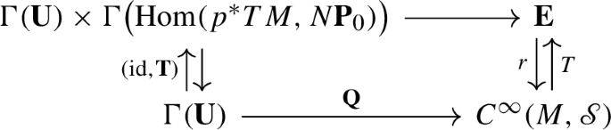
• (3) The derivative of ${\textbf{P}}_0 \in C^\infty (M,\mathscr {S})$ is a section $T{\textbf{P}}\in {{\,\textrm{Hom}\,}}(TM,{\textbf{P}}_0^*T\mathscr {S})$. Therefore, differentiation defines a section $T \in \Gamma ({\textbf{E}})$ of the vector bundle

  $$\begin{aligned} r :{\textbf{E}}:=\coprod _{{\textbf{P}}_0 \in C^\infty (M,\mathscr {S})} \Gamma \big ({{{\,\textrm{Hom}\,}}(TM,{\textbf{P}}_0^*T\mathscr {S})}\big ) \rightarrow C^\infty (M,\mathscr {S}). \end{aligned}$$

  Let $\varvec{\jmath }:{\textbf{U}}\looparrowright M \times Y$ be a tubular neighborhood of ${\textbf{P}}_0$. The map ${\textbf{Q}}_{\varvec{\jmath }} :\Gamma ({\textbf{U}}) \rightarrow C^\infty (M,\mathscr {S})$ defined by

  $$\begin{aligned} {\textbf{Q}}_{\varvec{\jmath }}(v)(x) :={\textbf{Q}}_{\jmath _x}(v) \quad \text {with}\quad v_x :=v|_{{\textbf{P}}_0(x)} \end{aligned}$$

  is (the inverse of) a chart on $C^\infty (M,\mathscr {S})$. Within this chart ${\textbf{E}}$ is trivialised and T is identified with a smooth map ${\textbf{T}}= {\textbf{T}}_{\varvec{\jmath }} \in C^\infty \Big ({\Gamma ({\textbf{U}}),\Gamma \big ({{{\,\textrm{Hom}\,}}(p^*TM,N{\textbf{P}}_0)}\big )}\Big )$; that is: the diagram

  

  commutes. (See Fig. 1 and Remark 3.16.)

Henceforth, suppose that $\phi _0$ is a $G_2$–structure and that ${\textbf{P}}_0(x)$ is $\phi _0$–associative for every $x \in M$.

• (4) Define $D = D_{{\textbf{P}}_0} :\Gamma (N{\textbf{P}}_0) \rightarrow \Gamma (N{\textbf{P}}_0)$ by

  $$\begin{aligned} (D v)|_{{\textbf{P}}_0(x)} :=D_{{\textbf{P}}_0(x)} \left( {v|_{{\textbf{P}}_0(x)}}\right) . \end{aligned}$$

  Set

  $$\begin{aligned} \mathscr {V}:=\left\{ v \in \Gamma (N{\textbf{P}}_0): v|_{{\textbf{P}}_0(x)} \perp _{L^2} {{\,\textrm{im}\,}}T_x{\textbf{P}}_0 ~\text {for every}~ x \in M \right\} \end{aligned}$$

  with $\perp _{L^2}$ denoting $L^2$ orthogonality. Denote by $D^\perp = D_{{\textbf{P}}_0}^\perp :\mathscr {V}\rightarrow \mathscr {V}$ the map induced by D and projection onto $\mathscr {V}$.

• (5) Let $\varvec{\jmath }:{\textbf{U}}\looparrowright M \times Y$ be a tubular neighborhood of ${\textbf{P}}_0$. Define $\mathscr {N}= \mathscr {N}_{\varvec{\jmath }} \in C^\infty (\Gamma ({\textbf{U}}),\Gamma (N{\textbf{P}}_0))$ by

  $$\begin{aligned} (\mathscr {N}v)|_{{\textbf{P}}_0(x)} :=\mathscr {N}_{\jmath _x} \left( {v}\right) |_{{\textbf{P}}_0(x)}. \end{aligned}$$

  $\bullet$

Remark 3.16

The upcoming Proposition 3.19 constructs a perturbation ${\textbf{P}}:={\textbf{Q}}_{\varvec{\jmath }}(v)$ of ${\textbf{P}}_0$. To establish one of the desired properties of ${\textbf{P}}$, it is necessary to compare the derivatives $T{\textbf{P}}$ and $T{\textbf{P}}_0$. The purpose of the map ${\textbf{T}}$ is to enable this. $\clubsuit$

Fig. 1

A sketch of the situation of Definition 3.15 (3).

Example 3.17

In the situation of Example 3.2 with $\mu = \textrm{id}_\Sigma$, $M = T^2$, $\underline{{\textbf{P}}}_0 = T^2 \times (S^1 \times \Sigma )$ and $N{\textbf{P}}_0 = TT^2 \oplus N\Sigma$. $D_{{\textbf{P}}_0(x)}$ and $\mathscr {N}_{\jmath _x}$—for a suitable choice of $\varvec{\jmath }$ and with respect to suitable identifications—are independent of $x \in T^2$.

Definition 3.18

Let ${\textbf{P}}_0 :M \rightarrow \mathscr {S}$ be a smooth map. Suppose that Riemannian metrics on M and Y are given. This induces a Euclidean inner product and an orthogonal covariant derivative $\nabla$ on $N{\textbf{P}}_0 \rightarrow \underline{{\textbf{P}}}_0$, and an Ehresmann connection on $p :\underline{{\textbf{P}}}_0 \rightarrow M$. Denote by $\nabla ^{1,0}$ and $\nabla ^{0,1}$ the restriction of $\nabla$ to the horizontal and vertical directions defined by the Ehresmann connection respectively. Denote by

$$\begin{aligned} {\mathfrak P}:=\coprod _{x \in M} C^\infty ([0,1],p^{-1}(x)) \end{aligned}$$

the set of vertical paths in $p :\underline{{\textbf{P}}}_0 \rightarrow M$. Denote by ${\mathfrak P}^+ \subset {\mathfrak P}$ the subset of non-constant paths. For $\alpha \in (0,1)$ set

$$\begin{aligned}{}[v]_{C^0C^{0,\alpha }} :=\sup _{\gamma \in {\mathfrak P}^+} \frac{|{{\,\textrm{tra}\,}}_\gamma (v(\gamma (0)))-v(\gamma (1))|}{\ell (\gamma )^\alpha } \quad \text {and}\quad \Vert v\Vert _{C^0C^{0,\alpha }} :=\Vert v\Vert _{C^0} + [v]_{C^0C^{0,\alpha }} \end{aligned}$$

with $\ell (\gamma )$ denoting the length of $\gamma$ and ${{\,\textrm{tra}\,}}_\gamma$ denoting parallel transport along $\gamma$. For $k,\ell \in {\textbf{N}}_0,\alpha \in (0,1)$ define the norm $\Vert -\Vert _{C^kC^{\ell ,\alpha }}$ on $\Gamma (N{\textbf{P}}_0)$ by

$$\begin{aligned} \Vert v\Vert _{C^kC^{\ell ,\alpha }} :=\sum _{m=0}^k \sum _{n=0}^\ell \Vert \left( {\nabla ^{1,0}}\right) ^m\left( {\nabla ^{0,1}}\right) ^n v\Vert _{C^0C^{0,\alpha }}. \end{aligned}$$

$\bullet$

Proposition 3.19

Let $\alpha \in (0,1)$, $\beta ,\gamma ,c_1,c_2,c_3,c_4,c_5,R > 0$. If $\beta > 2\gamma$, then there are constants $T = T(\alpha ,\beta ,\gamma ,c_1,c_2,c_3,c_4,c_5,R) > 0$ and $c_v = c_v(\alpha ,\beta ,\gamma ,c_1,c_2,c_3) > 0$ with the following significance. Let $\phi _0, \phi \in \Omega ^3(Y)$ be two $G_2$–structures on Y. Let ${\textbf{P}}_0 :M \rightarrow \mathscr {S}$ be a Morse–Bott family of $\phi _0$–associative submanifolds. Let $\varvec{\jmath } :{\textbf{U}}\looparrowright M \times Y$ be a tubular neighborhood of ${\textbf{P}}_0$. Let $t \in (0,T)$. Suppose that:

• (1) $B_R(0) \subset U_x$.

• (2) $\Vert \varvec{\jmath }^*(\phi -\phi _0)\Vert _{C^{1,\alpha }({\textbf{U}})} \le c_1 t^\beta$.

• (3) $D^\perp :\mathscr {V}\rightarrow \mathscr {V}$ is bijective and

  $$\begin{aligned} \Vert v\Vert _{C^1C^{1,\alpha }} \le c_2 t^{-\gamma } \Vert D^\perp v\Vert _{C^1C^{0,\alpha }}. \end{aligned}$$

• (4) $\mathscr {N}\in C^\infty (\Gamma ({\textbf{U}}),\Gamma (N{\textbf{P}}_0))$ satisfies

  $$\begin{aligned} \Vert \mathscr {N}(v)-\mathscr {N}(w)\Vert _{C^1C^{0,\alpha }} \le c_3 ({\Vert v\Vert _{C^1C^{1,\alpha }}+\Vert w\Vert _{C^1C^{1,\alpha }}})\Vert v-w\Vert _{C^1C^{1,\alpha }}. \end{aligned}$$

• (5) For every $\hat{x} \in T M$ and $v \in \Gamma ({\textbf{U}})$

  $$\begin{aligned} |\hat{x}| \le c_4 \Vert {\textbf{T}}(0)(\hat{x})\Vert _{C^0} \quad \text {and}\quad \Vert {\textbf{T}}(v) - {\textbf{T}}(0)\Vert _{C^0} \le c_5\Vert v\Vert _{C^1C^{1,\alpha }}. \end{aligned}$$

In this situation, there is a $v \in \Gamma ({\textbf{U}}) \subset \Gamma (N{\textbf{P}}_0)$ with $\Vert v\Vert _{C^1C^{1,\alpha }} \le c_vt^{\beta -\gamma }$ such that the map

$$\begin{aligned} {\textbf{P}}:={\textbf{Q}}_{\varvec{\jmath }}(v) :M \rightarrow \mathscr {S}\end{aligned}$$

(3.20)

is transverse to $\ker \delta \Upsilon ^\psi$ (as in Lemma 3.6).

Moreover, if H is a finite group acting on M and Y, $\phi _0$ and $\phi$ are H–invariant, and $\varvec{\jmath }$ and ${\textbf{P}}_0$ are H–equivariant, then ${\textbf{P}}$ is H–equivariant.

Remark 3.21

The condition (3) can be understood as a quantification of the Morse–Bott condition.

Proof of Proposition 3.19

To ease notation, define $f_0,f \in C^\infty (\Gamma ({\textbf{U}}),\Gamma (N{\textbf{P}}_0))$ by

$$\begin{aligned} \left\langle f_0(v)|_{{\textbf{P}}_0(x)},w\right\rangle _{L^2} :=\left\langle {{\textbf{Q}}_{\jmath _x}^*(\delta \Upsilon ^{\psi _0})}(v),w\right\rangle \quad \text {and}\quad \left\langle f(v)|_{{\textbf{P}}_0(x)},w\right\rangle _{L^2} :=\left\langle {{\textbf{Q}}_{\jmath _x}^*(\delta \Upsilon ^\psi )}(v),w\right\rangle . \end{aligned}$$

Denote by $(-)^\perp$ the projection onto $\mathscr {V}$. For every $v \in \mathscr {V}$

$$\begin{aligned} (D^\perp )^{-1}f(v)^\perp = v + \underbrace{(D^\perp )^{-1}\left( {\mathscr {N}(v) + f(v) - f_0(v)}\right) ^\perp }_{:=E(v)}. \end{aligned}$$

By (2), (3), and (4), there is a constant $c_E = c_E(\alpha ,\beta ,\gamma ,c_1,c_2,c_3) > 0$ such that for every $r \in (0,R)$ and $v,w \in \overline{B}_r(0) \subset C^1C^{1,\alpha }\Gamma (N{\textbf{P}}_0)$

$$\begin{aligned} \Vert E(0)\Vert _{C^1C^{1,\alpha }}&\le c_Et^{\beta -\gamma } \quad \text {and}\\ \Vert E(v) - E(w)\Vert _{C^1C^{1,\alpha }}&\le c_E(r+t^{\beta })t^{-\gamma } \Vert v-w\Vert _{C^1C^{1,\alpha }}. \end{aligned}$$

Therefore, $-E$ defines a contraction on $\overline{B}_r(0) \subset C^1C^{1,\alpha }\Gamma (N{\textbf{P}}_0)$ provided

$$\begin{aligned} c_E(r + t^\beta )t^{-\gamma } < 1 \quad \text {and}\quad c_E t^{\beta -\gamma } + c_E(r + t^\beta )t^{-\gamma } r \le r. \end{aligned}$$

These can be seen to hold for $r :=2c_Et^{\beta -\gamma }$ and $t \le T \ll 1$ because $\beta > 2\gamma$. Denote by $v \in \overline{B}_r(0) \subset C^1C^{1,\alpha }\Gamma (N{\textbf{P}}_0)$ the unique solution of

$$\begin{aligned} f(v)^\perp = 0. \end{aligned}$$

By elliptic regularity, $v \in \Gamma ({\textbf{U}})$.

It remains to prove that ${\textbf{P}}$ defined by (3.20) is transverse to $\ker \delta \Upsilon ^\psi$; that is: for every $x \in M$

$$\begin{aligned} \ker (\delta \Upsilon ^\psi )_{{\textbf{P}}(x)} + {{\,\textrm{im}\,}}T_x{\textbf{P}}= T_{{\textbf{P}}(x)}\mathscr {S}, \end{aligned}$$

or, equivalently,

$$\begin{aligned} f_x(v) = 0 \quad \text{ or }\quad f_x(v) \notin \left( {{{\,\text {im}\,}}{{\textbf {T}}}_x(v)}^\perp \right) . \end{aligned}$$

Here the subscript x indicates restriction to ${\textbf{P}}_0(x)$. By construction, $f_x(v) \in {{\,\textrm{im}\,}}{\textbf{T}}_x(0)$. Therefore, the hypothesis is satisfied by (5) provided $t \le T \ll 1$.

Evidently, this construction preserves H–equivariance. $\square$

In Example 3.2 with $\Sigma = S^2$, the following gives the required estimate on D.

Situation 3.22

Let X be a compact oriented Riemannian manifold. Let V be a Euclidean vector bundle over X. Let $A :\Gamma (V) \rightarrow \Gamma (V)$ be a formally self-adjoint linear elliptic differential operator of first order. Denote by $\pi :\Gamma (V) \rightarrow \ker A$ the $L^2$ orthogonal projection onto $\ker A$. Let $L > 0$. Define $\Pi :\Gamma \left( {(\textbf{R}/L\textbf{Z}) \times X,V}\right) \rightarrow \ker A$ by

with $i_t(x) :=(t,x)$.

Remark 3.23

In the situation of Example 3.2 with $\mu = \textrm{id}_\Sigma$, according to Example 3.13

$$\begin{aligned} D_{P_{[\eta ]}} = (-i\oplus I_\xi )\cdot (\partial _\xi +A) \quad \text {with}\quad A :=\begin{pmatrix} 0 &{} i\bar{\partial }^*\kappa ^* \\ -\kappa \bar{\partial }i &{} 0 \end{pmatrix}. \end{aligned}$$

$\clubsuit$

Proposition 3.24

In Situation 3.22, for every $\alpha \in (0,1)$ there is a constant $c = c(A,\alpha ) > 0$ such that for every $s \in \Gamma ((\textbf{R}/L\textbf{Z}) \times X,V)$

$$\begin{aligned} \Vert s\Vert _{C^{1,\alpha }} \le c\big ({(L+1)\Vert (\partial _t+A)s\Vert _{C^{0,\alpha }} + \Vert \Pi s\Vert _{L^\infty }}\big ). \end{aligned}$$

Proof

By interior Schauder estimates

$$\begin{aligned} \Vert s\Vert _{C^{1,\alpha }} \le c_1\left( {\Vert (\partial _t+A)s\Vert _{C^{0,\alpha }} + \Vert s\Vert _{L^\infty }}\right) ; \end{aligned}$$

see, e.g., [Kic06, §3]. Define $\hat{\pi }:\Gamma ((\textbf{R}/L\textbf{Z}) \times X,V) \rightarrow \Gamma ((\textbf{R}/L\textbf{Z}) \times X,V)$ by

$$\begin{aligned} (\hat{\pi }s)(t,x) :=\left( {\pi (i_t^*s)}\right) (x). \end{aligned}$$

A contradiction argument proves that

$$\begin{aligned} \Vert (\textbf{1}-\hat{\pi })s\Vert _{L^\infty } \le c_2\Vert (\partial _t+A)(\textbf{1}-\hat{\pi })s\Vert _{C^{0,\alpha }} \le c_2\big ({\Vert (\partial _t+A)s\Vert _{C^{0,\alpha }} + \Vert (\partial _t+A)\hat{\pi }s\Vert _{C^{0,\alpha }}}\big ); \end{aligned}$$

cf. [Wal13, Proof of Proposition 8.5]. As a consequence of the fundamental theorem of calculus

$$\begin{aligned} \Vert \hat{\pi }s\Vert _{L^\infty } \le L\Vert \partial _t \hat{\pi }s\Vert _{L^\infty } + \Vert \Pi s\Vert _{L^\infty } = L\Vert (\partial _t+A)\hat{\pi }s\Vert _{L^\infty } + \Vert \Pi s\Vert _{L^\infty }. \end{aligned}$$

Therefore,

$$\begin{aligned} \Vert s\Vert _{L^\infty } \le c_2\Vert (\partial _t+A)s\Vert _{C^{0,\alpha }} + (c_2+L)\Vert (\partial _t+A)\hat{\pi }s\Vert _{L^\infty } + \Vert \Pi s\Vert _{L^\infty }. \end{aligned}$$

Since A is formally self-adjoint,

$$\begin{aligned} \hat{\pi }(\partial _t + A) = (\partial _t + A)\hat{\pi }. \end{aligned}$$

Therefore,

$$\begin{aligned} \Vert (\partial _t+A)\hat{\pi }s\Vert _{C^{0,\alpha }} \le c_3\Vert (\partial _t+A)s\Vert _{C^{0,\alpha }}. \end{aligned}$$

The above observations combine to the asserted estimate with $c = c_1(c_2+1)(c_3+1)$. $\square$

4 Examples

The purpose of this section is to construct the associative submanifolds whose existence was promised in Sect. 1. These associative submanifolds are diffeomorphic to $S^1 \times S^2$, have not appeared in the literature (known to the authors) so far, and—most importantly— their volumes tend to zero as the ambient $G_2$–manifolds degenerate. In the following, some examples are exhibited. These are certainly not exhaustive; cf.Remark 4.7.

Here is a construction technique based on Proposition 3.19 and Remark 3.7 (2).

Proposition 4.1

Let ${\mathfrak R}= (\Gamma _\alpha ,G_\alpha ,\rho _\alpha ;R_\alpha ,\jmath _\alpha ;\hat{X}_\alpha ,\hat{\varvec{\omega {}}}_\alpha ,\hat{\rho }_\alpha ,\tau _\alpha )_{\alpha \in A}$ be resolution data for a closed flat $G_2$–orbifold $(Y_0,\phi _0)$. Denote by $(Y_t,\phi _t)_{t \in (0,T_0)}$ the family of closed $G_2$–manifolds obtained from the generalised Kummer construction discussed in Sect. 2. Let $\star \in A$, $\hat{\xi }\in S^2 \subset {\text {Im}}\textbf{H}$, $L > 0$, and $\Sigma \subset X_\star$. Set $\xi :=L\hat{\xi }$, $\Lambda _\star :=G_\star \cap {\text {Im}}\textbf{H}< {\text {Im}}\textbf{H}$, $M_\star :=\left( {{\text {Im}}\textbf{H}/\textbf{R}\xi }\right) /\left( {\Lambda _\star /\textbf{Z}\xi }\right)$, and $H_\star :=G_\star /\Lambda _\star$. Denote by ${\textbf{I}}_\star$ the hypercomplex structure on $X_\star$. Suppose that:

• (1) $\Sigma$ is a closed $I_{\star ,\hat{\xi }}$–holomorphic curve. $\Sigma \cong S^2$.

• (2) $\xi \in \Lambda _\star$ is primitive. $\textbf{Z}\xi < G_\star$ is normal.

• (3) $\rho _\star (g)(\Sigma ) = \Sigma$ for every $g \in G_\star$, and $\rho (\xi )|_\Sigma = \textrm{id}_\Sigma$.

Denote by $n_f$ the number of singularities of the orbifold $M_\star /H_\star$ (see Remark 3.3). In this situation, there is a constant $T_1 \in (0,T_0]$ and for every $t \in (0,T_1)$ there are at least $n_f$ distinct associative submanifolds in $(Y_t,\phi _t)$ representing the homology class $\beta :=\upsilon _\star ([P_{[0]}]) \in \textrm{H}_3(Y_t,\textbf{Z})$ with $\upsilon _\star$ as in Remark 2.17 and $P_{[0]} \subset \hat{Y}_{\star ,t}$ as in Example 3.2.

Proof

For every $[\eta ] \in M_\star /H_\star$ and $t \ll 1$, Example 3.2 constructs a $t^{-3}\tilde{\phi }_t$–associative submanifold $P_{[\eta ]} \looparrowright \hat{Y}_{\star ,t}^\circ {\setminus } \hat{V}_{\star ,t}$. This defines an $H_\star$–invariant Morse–Bott family ${\textbf{P}}_0 :M_\star \rightarrow \mathscr {S}$ of $t^{-3}\tilde{\phi }_t$–associative submanifolds; see Example 3.13. With respect to $t^{-2}{\tilde{g}}_t$ these submanifolds are isometric to $(\textbf{R}/t^{-1}L\textbf{Z}) \times \Sigma$.

The hypotheses of Proposition 3.19 are satisfied for the choices $\phi _0 = t^{-3}\tilde{\phi }_t$, $\phi = t^{-3}\phi _t$, $\alpha \in (0,1/16)$, $\beta = 5/2$, $\gamma = 1$, and choices of $c_1,c_2,c_3,c_4,c_5,R >0$ which shall not be specified (because of their secondary importance): (1) holds for $0 < R \ll 1$. (2) holds by Theorem 2.19. Because of Remark 2.18 (the proof of) Proposition 3.10 implies (4). For a suitable choice of $\varvec{\jmath }$, (5) holds with respect to $t^{-2}{\tilde{g}}_t$ by direct inspection; cf. Example 3.17. It remains to verify (3). As pointed out in Example 3.13, $N {\textbf{P}}_0([\eta ]) = T_{[\eta ]}M_\star \oplus N\Sigma$. Therefore, $N{\textbf{P}}_0 \cong TM_\star \oplus N\Sigma \rightarrow \underline{{\textbf{P}}}_0 \cong (\textbf{R}/t^{-1}L\textbf{Z}) \times \Sigma \times M_\star$. By Remark 3.23, $D_{{\textbf{P}}_0([\eta ])}$ is as in Situation 3.22. By definition, $v \in \mathscr {V}$ if $v|_{{\textbf{P}}_0([\eta ])} \perp _{L^2} {{\,\textrm{im}\,}}T_{[\eta ]}{\textbf{P}}_0 = T_{[\eta ]}M_\star$ for every $[\eta ] \in M_\star$. Since $\Sigma \cong S^2$, $\ker A = T_{[\eta ]}M_\star$ and the preceding condition is equivalent to $\Pi (v|_{{\textbf{P}}_0([\eta ])}) = 0$. Therefore, Proposition 3.24 implies (3) with respect to $t^{-2}{\tilde{g}}_t$.

For $t \in (0,T_{1/2})$ the resulting $H_\star$–invariant map ${\textbf {P}} :M_\star \rightarrow \mathscr {S}$ is transverse to $\ker \delta \Upsilon$ (as in Lemma 3.6). By Remark 3.7 (2), every isolated fixed-point of the action of $H_\star$ on $M_\star$ is a zero of ${\textbf{P}}^*(\delta \Upsilon ^{\phi _t})$. If $t < T_1 \ll T_{1/2}$, then these map to $n_f$ pairwise distinct elements of $\mathscr {S}$. By Lemma 3.6, each one of these is a $\phi _t$–associative submanifold. $\square$

Remark 4.2

If $x \in M_\star$ corresponds to an orbifold point $[x] \in M_\star /H_\star$, then $P_0 :={\textbf{P}}_0(x)$ and ${\textbf{P}}(x)$ are multiply covering and their deck transformation group contain the isotropy group $\Gamma$ of [x]. The embedded associative submanifold $\check{P}_0 :=P_0/\Gamma$ is unobstructed; indeed:

$$\begin{aligned} \ker D_{\check{P}_0} = (\ker D_{P_0})^\Gamma = (T_xM_\star )^\Gamma = 0. \end{aligned}$$

This can be used to give a somewhat simpler proof of most of Proposition 4.1 avoiding the use of Proposition 3.19.

Example 4.3

Joyce [Joy96b, Examples 4, 5, 6] constructs 7 examples of closed flat $G_2$–orbifolds $(Y_0,\phi _0)$ whose singular set has components $S_\alpha$ ($\alpha \in A$). A is a disjoint union $A = A^0 \amalg A^1$ with $A^1 \ne \emptyset$. For $\alpha \in A^0$, $S_\alpha$ is isometric to $T^3 :=\textbf{R}^3/\textbf{Z}^3$. For $\alpha \in A^1$, $S_\alpha$ is isometric to $T^3/C_2$. Here is a more precise description. For $\alpha \in A$ set $\Gamma _\alpha :=C_2$. For $\alpha \in A^0$ set $G_\alpha :=\Lambda = \left\langle i,j,k\right\rangle < {\text {Im}}\textbf{H}$ and denote by $\rho _\alpha :G_\alpha \rightarrow {{\,\textrm{Isom}\,}}(\textbf{H}/\Gamma _\alpha )$ the trivial homomorphism. For $\alpha \in A^1$ let $G_\alpha < \textrm{SO}({\text {Im}}\textbf{H}) < imes {\text {Im}}\textbf{H}$ be generated by $\Lambda$ and $(R_2,\frac{i}{2})$ with $R_2$ as in (2.5), and define $\rho _\alpha :G_\alpha \rightarrow G_\alpha /\Lambda \rightarrow N_{\textrm{SO}(\textbf{H})}(\Gamma _\alpha ) \hookrightarrow {{\,\textrm{Isom}\,}}(\textbf{H}/\Gamma _\alpha )$ by

$$\begin{aligned} \rho _\alpha \big ({R_2,\tfrac{i}{2}}\big )[q] :=[-iqi]. \end{aligned}$$

For every $\alpha \in A$ there is an open embedding $\jmath _\alpha :\big ({{\text {Im}}\textbf{H}\times \left( {B_{R_\alpha }(0)/\Gamma _\alpha }\right) }\big )/G_\alpha \hookrightarrow Y_0$ as in Definition 2.6 (2).

These can be extended to resolution data ${\mathfrak R}$ for $(Y_0,\phi _0)$ with the aid of the Gibbons–Hawking construction discussed in Remark 2.12. According to Remark 2.12 (2), $(X_{\varvec{0}},{\varvec{\omega {}}}_{\varvec{0}})$ is $\textbf{H}/C_2$ with the standard hyperkähler form. If ${\varvec{\zeta }}= [\zeta ,-\zeta ] \in \Delta ^\circ$, then $(X_{\varvec{\zeta }},{\varvec{\omega {}}}_\zeta )$ is a hyperkähler manifold and Remark 2.12 (2) provides $\tau :X_{{\varvec{\zeta }}}{\setminus } K_{\varvec{\zeta }}\rightarrow X_{\varvec{0}}$. Therefore, completing the resolution data for $\alpha \in A^0$ amounts to a choice of $\zeta _\alpha \in \Delta ^\circ$

For $\alpha \in A^1$ the situation is slightly complicated by the fact that $\rho _\alpha$ is non-trivial. The involution $R(q) :=-iqi$ lies in and $\Lambda ^+R = R_2$. By Remark 2.12 (4), requiring that R lifts to $X_{\varvec{\zeta }}$ imposes the constraint that ${\varvec{\zeta }}_\alpha \in (\Delta ^\circ )^{R_2}$. Therefore, completing the resolution data for $\alpha \in A^1$ amounts to a choice of ${\varvec{\zeta }}_\alpha \in (\Delta ^\circ )^{R_2}$. If

$$\begin{aligned} {\varvec{\zeta }}\in \left\{ [\zeta ,-\zeta ] \in \Delta ^\circ : \zeta \in {\textbf {R}}i \right\} \subset (\Delta ^\circ )^{R_2}, \end{aligned}$$

then the segment joining $\zeta$ and $-\zeta$ lifts to an $I_i$–holomorphic curve $\Sigma \cong S^2$. Therefore, for the corresponding choices of ${\mathfrak R}$, Proposition 4.1 with $\hat{\xi }= i$ and $L = 1$ exhibits 4 associative submanifolds in $(Y_t,\phi _t)$ for every $t \in (0,T_1)$.

Example 4.4

Joyce [Joy96b, Examples 15, 16] constructs two examples of closed flat $G_2$–orbifolds $(Y_0,\phi _0)$ whose singular set has components $S_\alpha$ ($\alpha \in A$). A is a disjoint union $A = A^0 \amalg A^1$ with $A^1 = \left\{ \star \right\}$. The situation is analogous to that in Example 4.3 except that $\Gamma _\star :=C_3$.

Completing the resolution data for $\star$ amounts to a choice of ${\varvec{\zeta }}_\star \in (\Delta ^\circ )^{R_2}$ with $R_2$ as in (2.5). If

$$\begin{aligned} {\varvec{\zeta }}\in \left\{ [\zeta _1,\zeta _2,\zeta _3] \in \Delta ^\circ : \zeta _1,\zeta _2,\zeta _3 \in {\textbf {R}}i \right\} \subset (\Delta ^\circ )^{R_2} \end{aligned}$$

and $\zeta _2$ is contained in the segment joining $\zeta _1$ and $\zeta _2$, then the segment joining $\zeta _1$ and $\zeta _2$ and the segment joining $\zeta _2$ and $\zeta _3$ lift to $I_{\star ,i}$–holomorphic curves $\Sigma _1,\Sigma _2 \cong S^2$ and Proposition 4.1 (2) holds. Therefore, for the corresponding choices of ${\mathfrak R}$, Proposition 4.1 with $\hat{\xi }= i$ and $L = 1$ exhibits $8 = 2\cdot 4$ associative submanifolds in $(Y_t,\phi _t)$ for every $t \in (0,T_1)$.

Example 4.5

Reidegeld [Rei17, §5.3.4] constructs an example of a closed flat $G_2$–orbifold $(Y_0,\phi _0)$ whose singular set has 16 components $S_\alpha$ ($\alpha \in A$). For every $\alpha \in A$, $S_\alpha$ is isometric to $T^3/C_2^2$. Here is a more precise description. For $\alpha \in A$ set $\Gamma _\alpha :=C_2$, let $G_\alpha < \textrm{SO}({\text {Im}}\textbf{H}) < imes {\text {Im}}\textbf{H}$ be generated by $\Lambda :=\left\langle i,j,k\right\rangle$, $(R_+,\frac{i+k}{2})$, and $(R_-,\frac{j}{2})$ with $R_\pm$ as in (2.5), define $\rho _\alpha :G_\alpha \rightarrow G_\alpha /\Lambda \rightarrow N_{\textrm{SO}(\textbf{H})}(\Gamma _\alpha ) \hookrightarrow {{\,\textrm{Isom}\,}}(\textbf{H}/\Gamma _\alpha )$ by

$$\begin{aligned} \rho _\alpha \big ({R_+,\tfrac{i+k}{2}}\big )[q] :=[iqi] \quad \text {and}\quad \rho _\alpha \big ({R_-,\tfrac{j}{2}}\big )[q] :=[jqj]. \end{aligned}$$

These act on ${\text {Im}}\textbf{H}$ as $R_+$ and $R_-$. For every $\alpha \in A$ there is an open embedding $\jmath _\alpha :\big ({{\text {Im}}\textbf{H}\times \left( {B_{R_\alpha }(0)/\Gamma _\alpha }\right) }\big )/G_\alpha \hookrightarrow Y_0$ as in Definition 2.6 (2).

Completing the resolution data for $\alpha \in A$ amounts to a choice of ${\varvec{\zeta }}_\alpha \in (\Delta ^\circ )^{R_+,R_-}$. If

$$\begin{aligned} {\varvec{\zeta }}\in \left\{ [\zeta ,-\zeta ] \in \Delta ^\circ : \zeta \in {\textbf {R}}i \right\} \subset (\Delta ^\circ )^{R_+,R_-}, \end{aligned}$$

then the segment joining $\zeta$ and $-\zeta$ lifts to an $I_i$–holomorphic curve $\Sigma \cong S^2$. Therefore, for every corresponding choice of ${\mathfrak R}$, Proposition 4.1 with $\hat{\xi }= i$ and $L = 1$ exhibits (up to 16 times) 2 associative submanifolds in $(Y_t,\phi _t)$ for every $t \in (0,T_1)$.

Example 4.6

Here is an example that involves non-cyclic $\Gamma$ and requires the use of Remark 2.15. Reidegeld [Rei17, §5.3.4] constructs an example of a closed flat $G_2$–orbifold $(Y_0,\phi _0)$ whose singular set has 7 components $S_\alpha$ ($\alpha \in A$). The situation is analogous to that in Example 4.5 except that $A = A^0 \amalg A^1 \amalg A^1$ and

$$\begin{aligned} \Gamma _\alpha :={\left\{ \begin{array}{ll} C_2 &{} \text {if}~\alpha \in A^0 \\ C_4 &{} \text {if}~\alpha \in A^1 \\ \textrm{Dic}_2 &{} \text {if}~\alpha \in A^2. \end{array}\right. } \end{aligned}$$

Completing the resolution data for $\alpha \in A^0$ is identical to Example 4.5. Completing the resolution data for $\alpha \in A^1$ amounts to a choice of ${\varvec{\zeta }}_\alpha \in (\Delta ^\circ )^{R_+,-R_-}$. The minus sign arises because $\alpha (R) = - 1$ for $R(q) = jqj$. If

$$\begin{aligned} {\varvec{\zeta }}\in \left\{ [\zeta _1,\zeta _2,\zeta _3,\zeta _4] \in \Delta ^\circ : \zeta _1,\zeta _2,\zeta _2,\zeta _4 \in {\textbf {R}}i \right\} \subset (\Delta ^\circ )^{R_+,-R_-} \end{aligned}$$

then $X_{\varvec{\zeta }}$ contains three $I_{{\varvec{\zeta }},i}$–holomorphic curves $\Sigma _a \cong S^2$ with $\hat{\xi }_a = \zeta _a/|\zeta _a|$ ($a=1,2$). Therefore, for the corresponding choices of ${\mathfrak R}$, Proposition 4.1 with $\hat{\xi }_a = i$ and $L = 1$ exhibits $6 = 3 \cdot 2$ associative submanifolds in $(Y_t,\phi _t)$ for every $t \in (0,T_1)$.

To understand the situation for $\alpha \in A^2$, recall that the $D_4$ root system is

$$\begin{aligned} \Phi = \left\{ \pm e_a \pm e_b \in {\textbf {R}}^4: a \ne b \in \left\{ 1,2,3,4 \right\} \right\} . \end{aligned}$$

The standard choice of simple roots is

$$\begin{aligned} \theta _1 :=e_1-e_2, \quad \theta _2 :=e_2-e_3, \quad \theta _3 :=e_3-e_4, \quad \text {and}\quad \theta _4 :=e_3+e_4. \end{aligned}$$

The Weyl group $W = S^4 < imes C_2^3$ acts by permuting and flipping the signs on an even number of the coordinates of $\textbf{R}^4$. Therefore,

$$\begin{aligned} \Delta ^\circ = \left\{ [\zeta _1,\zeta _2,\zeta _3,\zeta _4] \in ({\text{ Im }}{} {\textbf {H}}\otimes {\textbf {R}}^4)/W: \zeta _a \ne \pm \zeta _b ~\text{ for }~ a \ne b \in \left\{ 1,2,3,4 \right\} \right\} . \end{aligned}$$

The automorphism group of the Dynkin diagram is $S^3$, which fixes $\theta _2$ and permutes $\theta _1,\theta _3,\theta _4$. Since $\textrm{Dic}_2 = \left\langle i,j\right\rangle < \textrm{Sp}(1)$, for $R(q) = iqi$ and $R(q) = jqj$, $C_R \in {{\,\textrm{Aut}\,}}(\Gamma )$ is inner and, therefore, ${{\,\textrm{Ad}\,}}_{C_R}$ acts trivially on $\Phi$.

If

$$\begin{aligned} {\varvec{\zeta }}\in \left\{ [\zeta _1,\zeta _2,\zeta _3,\zeta _4] \in \Delta ^\circ : \zeta _1,\zeta _2,\zeta _3,\zeta _4 \in {\textbf {R}}i \right\} \subset (\Delta ^\circ )^{R_+,R_-}, \end{aligned}$$

then, by Remark 2.15 (4), $X_{\varvec{\zeta }}$ contains 4 $I_{{\varvec{\zeta }},i}$–holomorphic curves $\Sigma _a \cong S^2$ ($a \in \left\{ 1,2,3,4 \right\}$). Therefore, for the corresponding choices of ${\mathfrak R}$, Proposition 4.1 with $\hat{\xi }= i$ and $L = 1$ exhibits $8 = 4\cdot 2$ associative submanifolds in $(Y_t,\phi _t)$ for every $t \in (0,T_1)$.

Remark 4.7

(Homework assignment) Reidegeld [Rei17, §5.3.4 and §5.3.5] constructed further examples of closed flat $G_2$–orbifolds $(Y_0,\phi _0)$ whose singular sets are isometric to $T^3$, $T^3/C_2$, and $T^3/C_2^2$ and whose transverse singularity models are $\textbf{H}/\Gamma$ with $\Gamma \in \left\{ C_2,C_3,C_4,C_6,\textrm{Dic}_2,\textrm{Dic}_3,2T \right\}$. The reader might enjoy analysing these examples with the methods used above.

Here is a construction technique based on Proposition 3.19 and Remark 3.7 (3).

Proposition 4.8

Let ${\mathfrak R}= (\Gamma _\alpha ,G_\alpha ,\rho _\alpha ;R_\alpha ,\jmath _\alpha ;\hat{X}_\alpha ,\hat{\varvec{\omega {}}}_\alpha ,\hat{\rho }_\alpha ,\tau _\alpha ;\lambda _\alpha ,\kappa _\alpha ,\hat{\kappa }_\alpha )_{\alpha \in A}$ be K–equivariant resolution data for a closed flat $G_2$–orbifold $(Y_0,\phi _0)$ together with a homomorphism $\lambda :K \rightarrow {{\,\textrm{Diff}\,}}(Y_0)$ with respect to which $\phi _0$ is K–invariant. Denote by $(Y_t,\phi _t)_{t \in (0,T_0)}$ the family of closed $G_2$–manifolds obtained from the K–equivariant generalised Kummer construction discussed in Remark 2.20. Let $\star \in A$, $\hat{\xi }\in S^2 \subset {\text {Im}}\textbf{H}$, $L > 0$, and $\Sigma \subset X_\star$. Set $\xi :=L\hat{\xi }$, $\Lambda _\star :=G_\star \cap {\text {Im}}\textbf{H}< {\text {Im}}\textbf{H}$, and $M_\star :=\left( {{\text {Im}}\textbf{H}/\textbf{R}\xi }\right) /\left( {\Lambda _\star /\textbf{Z}\xi }\right)$. Denote by ${\textbf{I}}_\star$ the hypercomplex structure on $X_\star$. Suppose that (1), (2), and (3) in Proposition 4.1 hold; and moreover:

• (4) $g\star = \star$ for every $g \in K$, $\kappa _\star (K) < N_{\textrm{SO}({\text {Im}}\textbf{H}) < imes {\text {Im}}\textbf{H}}(\textbf{Z}\xi )$, and $\hat{\kappa }_\star (g)(\Sigma ) = \Sigma$ for every $g \in K$.

• (5) ${{\,\textrm{Hom}\,}}(\pi _1(M_\star ),\textbf{R})^K = 0$.

In this situation, there is a constant $T_1 \in (0,T_0]$ and for every $t \in (0,T_1)$ there are at least 3 distinct associative submanifolds in $(Y_t,\phi _t)$ representing the homology class $\beta :=\upsilon _\star ([P_{[0]}]) \in \textrm{H}_3(Y_t,\textbf{Z})$ with $\upsilon _\star$ as in Remark 2.17 and $P_{[0]} \subset \hat{Y}_{\star ,t}$ as in Example 3.2.

Proof

The proof is very similar to that of Proposition 4.1. The additional hypothesis (4) guarantees that K acts on $M_\star$ and that the map ${\textbf{P}}_0$ is K–equivariant. Therefore, ${\textbf{P}}$ is K–equivariant as well. According to Remark 3.7 (3), the obstruction to ${\textbf{P}}^*(\delta \Upsilon ^{\phi _t})$ being exact is the composite homomorphism

$$\begin{aligned} \pi _1(M_\star ) \xrightarrow {\pi _1({\textbf{P}})} \pi _1(\mathscr {S}) \xrightarrow {\text {sweep}} \textrm{H}_4(Y_t) \xrightarrow {\left\langle -,[\psi _t]\right\rangle } \textbf{R}. \end{aligned}$$

The first two homomorphisms are manifestly K–equivariant. The third homomorphism is K–equivariant because $\psi _t$ is K–invariant (see Remark 2.20). By (5), the composition vanishes. Therefore, ${\textbf{P}}^*(\delta \Upsilon ^{\phi _t})$ is exact. Since $M_\star \not \cong S^2$, ${\textbf{P}}^*(\delta \Upsilon ^{\phi _t})$ has at least 3 zeros.

$\square$

Example 4.9

Set $T^7 :=\textbf{R}^7/\textbf{Z}^7$. Define the torsion-free $G_2$–structure $\phi _0$ by

$$\begin{aligned}{} & {} \phi _0 :=\textrm{d}x_1 \wedge \textrm{d}x_2 \wedge \textrm{d}x_3 - \sum _{a=1}^3 \textrm{d}x_a \wedge \omega _a \quad \text {with} \\{} & {} \quad \omega _1 :=\textrm{d}x_4 \wedge \textrm{d}x_5 + \textrm{d}x_6 \wedge \textrm{d}x_7,\\{} & {} \quad \omega _2 :=\textrm{d}x_4 \wedge \textrm{d}x_6 + \textrm{d}x_7 \wedge \textrm{d}x_5, \quad \omega _3 :=\textrm{d}x_4 \wedge \textrm{d}x_7 + \textrm{d}x_5 \wedge \textrm{d}x_6. \end{aligned}$$

Define $\iota _1,\iota _2,\iota _3,\lambda \in {{\,\textrm{Isom}\,}}(T^7)$ by

$$\begin{aligned} \iota _1[x_1,\ldots ,x_7]&:=\left[ x_1,x_2,x_3,-x_4,-x_5,-x_6,-x_7\right] , \\ \iota _2[x_1,\ldots ,x_7]&:=\left[ x_1,-x_2,-x_3,x_4,x_5,\tfrac{1}{2}-x_6,-x_7\right] , \\ \iota _3[x_1,\ldots ,x_7]&:=\left[ -x_1,x_2,-x_3,x_4,\tfrac{1}{2}-x_5,x_6,\tfrac{1}{2}-x_7\right] , \quad \text{ and }\\ \lambda [x_1,\ldots ,x_7]&:=\left[ x_1,-x_2,-x_3,x_4,x_5,-x_6,-x_7\right] . \end{aligned}$$

$(Y_0 :=T^7/\left\langle \iota _1,\iota _2,\iota _3\right\rangle ,\phi _0)$ is the closed flat $G_2$–orbifold from [Joy96b, Example 3]. Its singular set has $12 = 3\cdot 4$ components $S_\alpha$ ($\alpha \in A = A^1 \amalg A^2 \amalg A^3$). Here $A^a$ groups those components arising from the fixed-point set of $\iota _a$. The situation is analogous to that in Example 4.3 except that, for every $\alpha \in A$, $S_\alpha$ is isometric to $T^3$ and $G_\alpha :=\Lambda = \left\langle i,j,k\right\rangle < {\text {Im}}\textbf{H}$.

The involution $\lambda$ descends to $Y_0$: it can be identified with an action of $C_2$ on $Y_0$ as in Remark 2.20. The induced action on A fixes the elements of $A^1$ and permutes those of $A^2$ and $A^3$. Completing the $C_2$–equivariant resolution data for $\alpha \in A^2 \amalg A^3$ presents no difficulty. For $\alpha \in A^1$, $\lambda _\alpha = R_2$ as in (2.5), and $\rho _\alpha (q) = -iqi$ as in Example 4.3. Therefore, completing the resolution data for $\alpha \in A^1$ amounts to a choice of

$$\begin{aligned} {\varvec{\zeta }}_\alpha \in (\Delta ^\circ )^{R_2} = \left\{ [\zeta ,-\zeta ] \in \Delta ^\circ : \zeta \in {\textbf {R}}i \cup ({\textbf {R}}i)^\perp \right\} . \end{aligned}$$

If ${\varvec{\zeta }}_\alpha = [\zeta _\alpha ,-\zeta _\alpha ]$ with $\zeta _\alpha \in \textbf{R}i$, then the hypotheses of Proposition 4.8 are satisfied with $\hat{\xi }= i$, $L = 1$, and $\Sigma$ as in Example 4.3; indeed: $C_2$ acts on $T^2$ by $[x_2,x_3] \mapsto [-x_2,-x_3]$; hence: ${{\,\textrm{Hom}\,}}(\pi _1(T^2),\textbf{R})^{C_2} = 0$. This exhibits up to $12 = 4 \cdot 3$ associative submanifolds in $(Y_t,\phi _t)$ for every $t \in (0,T_1)$ depending on the choice of $C_2$–equivariant resolution data.

Remark 4.10

If X is a K3 surface with a non-symplectic involution $\tau$, then the fixed-point locus $X^\tau$ (typically) contains a surface of genus $g \ne 1$ [Nik83, §4]. The twisted connected sum construction [Kov03, KL11, CHNP15]—in fact: a trivial version thereof—produces closed $G_2$–orbifolds $(Y_0,\phi _0)$ from a matching pair of K3 surfaces $\Sigma _\pm$ equipped with non-symplectic involutions $\tau _\pm$. The singular set of $Y_0$ is $S^1 \times M$ with $M :=X_+^\tau \cup X_-^\tau$ and the transverse singularity model is $\textbf{H}/C_2$. An extension of the generalised Kummer construction due to Joyce and Karigiannis [JK17] resolves $Y_0$ into a family $(Y_t,\phi _t)_{t\in (0,T_0)}$ of closed $G_2$–manifolds. It seems plausible that an extension of the techniques in the present article could produce ${\textbf{P}}:M \rightarrow \mathscr {S}$ transverse to $\ker \delta \Upsilon$ (as in Lemma 3.6). Since (typically) $\chi (M) \ne 0$, this would produce associatives in Joyce and Karigiannis’s $G_2$–manifolds.

Remark 4.11

It is also possible to construct coassociative submanifolds in $G_2$–manifolds obtained from the generalised Kummer construction using similar techniques. In fact, the situation is quite a bit simpler because the deformation theory of coassociative submanifolds is always unobstructed [McL98, §4]. Details and examples will appear in the forthcoming work of Gutwein [Gut22].

References

Acharya, B.S., Braun, A.P., Svanes, E.E., Valandro, R.: Counting associatives in compact \(G_2\) orbifolds. J. High Energy Phys. (2019). https://doi.org/10.1007/jhep03(2019)138
Akbulut, S., Salur, S.: Deformations in \(G_2\) manifolds. Adv. Math. 217(5), 2130–2140 (2008). https://doi.org/10.1016/j.aim.2007.09.009
Ball, G., Madnick, J.: Associative Submanifolds of the Berger Space (2020) arXiv: 2003.13169. to appear in Communications in Analysis and Geometry
Barbosa, R.: Harmonic Higgs Bundles and Coassociative ALE Fibrations (2019). arXiv: 1910.10742
Barrett, A.B.: \(M\)-Theory on Manifolds with \(G_2\) holonomy. PhD thesis. University of Oxford, (2006). arXiv: hep-th/0612096
Bera, G.: Deformations and gluing of asymptotically cylindrical associatives (2022). arXiv: 2209.00156
Braun, A.P., Del Zotto, M., Halverson, J., Larfors, M., Morrison, D.R., Schafer-Nameki, S.: Infinitely many M2-instanton corrections to M-theory on \(G_2\)-manifolds. J. High Energy Phys. (2018). https://doi.org/10.1007/jhep09(2018)077
Conway, J.H., Rossetti, J.P.: Describing the platycosms (2003). arXiv:math/0311476
Corti, A., Haskins, M., Nordström, J., Pacini, T.: \(G_2\)-manifolds and associative submanifolds via semi-Fano 3.folds. Duke Math. J. 164(10), 1971–2092 (2015). https://doi.org/10.1215/00127094-3120743
Doan, A., Walpuski, T.: On counting associative submanifolds and Seiberg.Witten monopoles. Pure Appl. Math. Quart. 15(4), 1047–1133 (2019). https://doi.org/10.4310/PAMQ.2019.v15.n4.a4
Donaldson, S.K., Segal, E.P.: Gauge theory in higher dimensions, II. Surveys in differential geometry. Vol. 16. Geometry of special holonomy and related topics. International Press, pp. 1–41. (2011) arXiv: 0902.3239
Donaldson, S.K., Thomas, R.P.: Gauge theory in higher dimensions. The geometric universe. Oxford University Press, pp. 31–47 (1998)
Gayet, D.: Smooth moduli spaces of associative submanifolds. Quart. J. Math. 65(4), 1213–1240 (2014). https://doi.org/10.1093/qmath/hat042
Gibbons, G.W., Hawking, S.W.: Gravitational multi-instantons. Phys. Lett. 78B, 430–432 (1978). https://doi.org/10.1016/0370-2693(78)90478-1
Gibbons, G.W., Rychenkova, P., Goto, R.: HyperKahler Quotient Construction of BPS Monopole Moduli Spaces. Commun. Math. Phys. 186(3), 581–599 (1997). https://doi.org/10.1007/s002200050121
Gutwein, D.: Coassociative submanifolds in Joyce’s generalised Kummer constructions. in preparation. (2022)
Halverson, J., Morrison, D.R.: On gauge enhancement and singular limits in \(G_2\) compactifications of M-theory. J. High Energy Phys. (2016). https://doi.org/10.1007/jhep04(2016)100
Hantzsche, W., Wendt, H.: Dreidimensionale euklidische Raumformen. Math. Ann. 110(1), 593–611 (1935). https://doi.org/10.1007/BF01448045
Harvey, R., Lawson, H.B., Jr.: Calibrated geometries. Acta Math. 148, 47–157 (1982). https://doi.org/10.1007/BF02392726
Haydys, A.: \(G_2\) instantons and the Seiberg.Witten monopoles (2017). arXiv:1703.06329
Joyce, D.D.: Compact Riemannian 7.manifolds with holonomy2. I. J. Differ. Geom. 43(2), 291–328 (1996). https://doi.org/10.4310/jdg/1214458109
Joyce, D.D.: Compact Riemannian 7.manifolds with holonomy.2. II. J. Differ. Geom. 43(2), 329–375 (1996). https://doi.org/10.4310/jdg/1214458110
Joyce, D.D.: Compact Manifolds with Special Holonomy. Oxford Mathematical Monographs. Oxford University Press, Oxford (2000)
Joyce, D.D.: Conjectures on counting associative 3-folds in \(G_2\)-manifolds. Modern geometry: a celebration of the work of Simon Donaldson. Proceedings of Symposia in Pure Mathematics 99. American Mathematical Society, pp. 97–160 (2018) https://doi.org/10.1090/pspum/099/01739
Joyce, D.D., Karigiannis, S.: A new construction of compact torsion-free. 2.manifolds by gluing families of Eguchi. Hanson spaces. J. Differ. Geom. 117(2), 255–343 (2017). https://doi.org/10.4310/jdg/1612975017
Kawai, K.: Some associative submanifolds of the squashed 7-sphere. Quart. J. Math. 66(3), 861–893 (2015). https://doi.org/10.1093/qmath/hav021
Kichenassamy, S.: Schauder-type estimates and applications. Handbook of Differential Equations: Stationary Partial Differential Equations. Vol. 3, pp. 401—464, Elsevier (2006) https://doi.org/10.1016/S1874-5733(06)80009-4
Klein, F.: Vorlesungen uber das Ikosaeder und die Auflosung der Gleichungen vom funften Grade. Reprint of the 1884 original (edited) with an introduction and commentary by P. Slodowy. Birkhauser Verlag, (1993). https://doi.org/10.1007/978-3-0348-8594-2
Kovalev, A.: Twisted connected sums and special Riemannian holonomy. J. Reine Angew. Math. 565, 125–160 (2003). https://doi.org/10.1515/crll.2003.097
Kovalev, A., Lee, N.-H.: \(K_3\) surfaces with non-symplectic involution and compact irreducible \(G_2\)-manifolds. Math. Proc. Camb. Philos. Soc. 151(2), 193–218 (2011). https://doi.org/10.1017/S030500411100003X
Kriegl, A., Michor, P.W.: The convenient setting of global analysis. Mathematical Surveys and Monographs 53. American Mathematical Society (1997). https://doi.org/10.1090/surv/053
Kronheimer, P.B.: A Torelli-type theorem for gravitational instantons. J. Differ. Geom. 29(3), 685–697 (1989)
Kronheimer, P.B.: The construction of ALE spaces as hyper-Kahler quotients. J. Differ. Geom. 29(3), 665–683 (1989)
Lotay, J.D.: Associative submanifolds of the 7.sphere. Proc. Lond. Math. Soc. 105(6), 1183–1214 (2012). https://doi.org/10.1112/plms/pds029
McDuff, D., Salamon, D.: J-Holomorphic Curves and Symplectic Topology, vol. 52, 2nd edn. American Mathematical Society Colloquium Publications. American Mathematical Society (2012)
McKay, J.: Graphs, singularities, and finite groups. The Santa Cruz Conference on Finite Groups. Proceedings of Symposia in Pure Mathematics 37. Amererican Mathematical Society, pp. 183–186.(1981) https://doi.org/10.1090/pspum/037
McLean, R.C.: Deformations of calibrated submanifolds. Commun. Anal. Geom. 6(4), 705–747 (1998). https://doi.org/10.4310/CAG.1998.v6.n4.a4
Milnor, J.W., Stasheff, J.D.: Characteristic classes. Annals of Mathematics Studies, No. 76. Princeton University Press; University of Tokyo Press, (1974)
Nikulin, V.V.: Factor groups of groups of automorphisms of hyperbolic forms with respect to subgroups generated by 2-reflections. Algebro-geometric applications. J. Sov. Math. 22, 1401–1475 (1983)
Platt, D.: Improved Estimates for \(G_2\)-structures on the Generalised Kummer Construction. (2022). arXiv: 2011.00482
Reidegeld, F.: \(G_2\)-Orbifolds with ADE-Singularities. Habilitation, TU Dortmund (2017)
Sa Earp, H.N., Walpuski, T.: \(G_2\)-instantons over twisted connected sums. Geom. Topol. 19(3), 1263–1285 (2015). https://doi.org/10.2140/gt.2015.19.1263
Salamon, D.A., Walpuski, T.: Notes on the octonions. In: Proceedings of the 23rd Gokova Geometry Topology Conference, pp. 1–85. (2017) arXiv: 1005.2820
Szczepański, A.: Geometry of crystallographic groups. Algebra and Discrete Mathematics 4. World Scientific Publishing, (2012). https://doi.org/10.1142/8519
Walpuski, T.: \(G_2\)-instantons on generalised Kummer constructions. Geom. Topol. 17(4), 2345–2388 (2013). https://doi.org/10.2140/gt.2013.17.2345
Walpuski, T.: \(G_2\)-instantons, associative submanifolds, and Fueter sections. Commun. Anal. Geom. 25(4), 847–893 (2017). https://doi.org/10.4310/CAG.2017.v25.n4.a4
Wilson, P.M.H.: The Kahler cone on Calabi. Yau threefolds. Invent. Math. 107(3), 561–583 (1992). https://doi.org/10.1007/BF01231902
Acknowledgements
This material is based upon work supported by the Simons Collaboration “Special Holonomy in Geometry, Analysis, and Physics” (DP, TW). The authors thank the referees and Dominik Gutwein for their careful reading and helpful suggestions.
Funding
Open Access funding enabled and organized by Projekt DEAL.
Author information
Authors and Affiliations
Corresponding author
Ethics declarations
Conflict of interest
The authors have no conflicts of interest to disclose.
Additional information
Publisher's Note
Springer Nature remains neutral with regard to jurisdictional claims in published maps and institutional affiliations.
Rights and permissions
Open Access This article is licensed under a Creative Commons Attribution 4.0 International License, which permits use, sharing, adaptation, distribution and reproduction in any medium or format, as long as you give appropriate credit to the original author(s) and the source, provide a link to the Creative Commons licence, and indicate if changes were made. The images or other third party material in this article are included in the article’s Creative Commons licence, unless indicated otherwise in a credit line to the material. If material is not included in the article’s Creative Commons licence and your intended use is not permitted by statutory regulation or exceeds the permitted use, you will need to obtain permission directly from the copyright holder. To view a copy of this licence, visit http://creativecommons.org/licenses/by/4.0/.
About this article
Cite this article
Dwivedi, S., Platt, D. & Walpuski, T. Associative Submanifolds in Joyce’s Generalised Kummer Constructions. Commun. Math. Phys. 401, 2327–2353 (2023). https://doi.org/10.1007/s00220-023-04716-7
Received:
Accepted:
Published:
Issue Date:
DOI: https://doi.org/10.1007/s00220-023-04716-7