A geometric approach to equivariant factorization homology and nonabelian Poincaré duality

Abstract

Fix a finite group G and an n-dimensional orthogonal G-representation V. We define the equivariant factorization homology of a V-framed smooth G-manifold with coefficients in an $\textrm{E}_V$-algebra using a two-sided bar construction, generalizing (Andrade, From manifolds to invariants of $E_n$-algebras. PhD thesis, Massachusetts Institute of Technology, 2010; Kupers and Miller, Math Ann 370(1–2):209–269, 2018). This construction uses minimal categorical background and aims for maximal concreteness, allowing convenient proofs of key properties, including invariance of equivariant factorization homology under change of tangential structures. Using a geometrically-seen scanning map, we prove an equivariant version (eNPD) of the nonabelian Poincaré duality theorem due to several authors. The eNPD states that the scanning map gives a G-equivalence from the equivariant factorization homology to mapping spaces out the one-point compactification of the G-manifolds, when the coefficients are G-connected. For non-G-connected coefficients, when the G-manifolds have suitable copies of $\mathbb {R}$ in them, the scanning map gives group completions. This generalizes the recognition principle for V-fold loop spaces in Guillou and May (Algebr Geom Topol 17(6):3259–3339, 2017).

Appendices

Appendix A. A comparison of scanning maps

The scanning map studied in Sect. 4.1 is a key input to the eNPD theorem. In this section we compare our scanning map (4.3) to other constructions.

Notation A.1

For a G-manifold M, $\textrm{Sph}(\textrm{T}M)$ is the G-space obtained by fiberwise one-point compatification of the tangent bundle of M. It is a fiber bundle over M with based fiber $S^n$, where the base point in each fiber is the point at infinity.

Non-equivariantly, people have used the name scanning map to refer to different but related constructions. In slogan, it is a map from the (fattened) configuration spaces of a manifold M to compactly defined sections of $\textrm{T}M$, or compactly supported sections of $\textrm{Sph}(\textrm{T}M)$. McDuff [30] was probably the first to study the scanning map for general manifolds. She thought of it as the field of the point charges and proved homological stability properties of this map.

When $\textrm{T}M \cong M \times V$, the situation is simpler and we have defined a scanning map in (4.4):

$$\begin{aligned} s_{S^0}: \coprod _{k \ge 0} \mathscr {D}_{M}^{\textrm{fr}_{V}}(k)/\Sigma _k \rightarrow \textrm{Map}_{c}(M, S^V). \end{aligned}$$

The left hand side is a model of the configuration space as justified in Proposition 3.30 (1); the right hand side is equivalent to the compactly supported sections of $\textrm{Sph}(\textrm{T}M) \cong M \times S^V$.

We are interested in the scanning maps of Manthorpe–Tillman and McDuff, both of which can be made equivariant without pain. The following table is a summary of the natural domains and codomains of each construction:

Scanning map	Domain	Codomain
This paper, s	Framed embeddings V to M	Maps $M^+$ to $S^V$
Manthorpe–Tillman, $\tilde{s}^{\textrm{MT}}$	Embeddings V to M	Sections of $\textrm{Sph}(\textrm{T}M)$
McDuff, $\tilde{s}^{\textrm{MD}}$	Configuration of points of M	Sections of $\textrm{Sph}(\textrm{T}M)$

In this section, we focus on the case of V-framed manifolds M. Then these maps have equivalent domains and identical codomains. We will show in Proposition A.7 and Proposition A.10 that:

Theorem A.2

The scanning maps $s_X$, $s_X^{\textrm{MD}}$ and $s_X^{\textrm{MT}}$ are G-homotopic after the change of domain.

Notation A.3

In the above and subsequent paragraphs,

• We use the letter s for scanning maps without labels and $s_X$ for labels in X.

• A tilde is put on s to denote when the codomain is the sections of $\textrm{Sph}(\textrm{T}M)$, that is, before composition with the framing.

• A superscript is put on s to distinguish between the different authors in the literature.

1.1 A.1. Scanning map from tubular neighborhood

Manthorpe–Tillman [33, Section 3.1] gave a map

$$\begin{aligned} \gamma ^{+}: \big ( \coprod _{k \ge 0} \textrm{Emb}(\amalg _k \mathbb {R}^n, M) \times _{\Sigma _{k}} X^{k} \big ) /\sim \ \rightarrow \textrm{Sect}_c(M, \textrm{Sph}(\textrm{T}M)\wedge _M \tau _{X}). \end{aligned}$$

Here, $\textrm{Sect}_c$ is the space of compactly supported sections; $\tau _X$ is the constant parametrized base space $X \times M$ over M and $\textrm{Sph}(\textrm{T}M)\wedge _M \tau _{X}$ is the fiberwise smashing of $\textrm{Sph}(\textrm{T}M)$ with X. (To translate, take their $M_0 = \varnothing$, $Y = W \times X$. Their $E_k(M,\pi )$ is the space $\textrm{Emb}(\amalg _k \mathbb {R}^n, M) \times _{\Sigma _{k}} X^{k}$, and their $\Gamma (W {\setminus } M_0, W {\setminus } M, \pi )$ is $\textrm{Sect}_c(M, \textrm{Sph}(\textrm{T}M)\wedge _M \tau _{X})$.)

The key feature of their construction is to exploit the data of the tubular neighborhood, so a framing on M is not needed. For example, when $k = 1$, we start with an embedding $f \in \textrm{Emb}(\mathbb {R}^n, M)$ and want to define $\gamma ^+(f)$, a compactly supported section of $\textrm{Sph}(\textrm{T}M)$. The image of f is a tubular neighborhood of the image of $0 \in V$ in M, and f induces an inclusion of bundles $df: \textrm{T}\mathbb {R}^n \rightarrow \textrm{T}M$. There is a canonical diagonal section $\mathbb {R}^{n} \rightarrow \mathbb {R}^n \times \mathbb {R}^n \cong \textrm{T}\mathbb {R}^n$. Pushing this section by df gives $\gamma ^+(f)$.

We can modify their $\gamma ^+$ by replacing $\mathbb {R}^n$ by the representation V to get

$$\begin{aligned} \gamma ^+_V:\textrm{Emb}_{M}(X) \equiv \big ( \coprod _{k \ge 0} \textrm{Emb}(\amalg _k V, M) \times _{\Sigma _{k}} X^{k} \big ) /\sim \ \rightarrow \textrm{Sect}_c(M, \textrm{Sph}(\textrm{T}M)\wedge _M \tau _{X}). \end{aligned}$$

We then precompose with the forgetting map $\textrm{D}_{M}^{\textrm{fr}_V} (X) \rightarrow \textrm{Emb}_{M}(X)$ in Remark 3.8 to get

$$\begin{aligned} \tilde{s}_{X}^{\textrm{MT}}: \textrm{D}_{M}^{\textrm{fr}_V} (X) \rightarrow \textrm{Sect}_c(M, \textrm{Sph}(\textrm{T}M)\wedge _M \tau _{X}). \end{aligned}$$

(A.4)

We describe how $\tilde{s}^{\textrm{MT}}_X$ works on the subspace $k=1$ and it is similar on the whole space. For the element $\bar{f}=(f, \alpha ) \in \textrm{Emb}^{\textrm{fr}_V}(V, M)$, we take the embedding $f: V \rightarrow M$. The derivative map of f is $df: \textrm{T}V \cong V \times V \rightarrow \textrm{T}M$. For each $m \in \textrm{image}(f)$, we need a vector $\tilde{s}^{\textrm{MT}}(f) \in \textrm{T}_mM$ that is determined by f. Denote $v = f^{-1}(m) \in V$. We have $df(v,-): V \cong \textrm{T}_vV \rightarrow \textrm{T}_mM$. Then the explicit formulas without or with labels are given by

$$\begin{aligned} \tilde{s}^{\textrm{MT}}(\bar{f})(m) = df(v,v) \quad \text {and} \quad \tilde{s}^{\textrm{MT}}_X(\bar{f},x)(m) = df(v,v) \wedge x. \end{aligned}$$

(A.5)

Both of them are G-maps.

The V-framing $\phi _M: \textrm{T}M \rightarrow V$ induces $\textrm{Sph}(\textrm{T}M) \wedge _M \tau _X \cong M \times \Sigma ^VX$. So we obtain a map which we still call the scanning map:

$$\begin{aligned} s^{\textrm{MT}}_{X} :\textrm{D}_{M}^{\textrm{fr}_V} (X) \rightarrow \textrm{Map}_c(M, \Sigma ^VX). \end{aligned}$$

(A.6)

A prior, this scanning map is different from the scanning map (4.2) in Sect. 4.1. For an element $\bar{f}=(f,\alpha )$ where $f: V \rightarrow M$ with $f(v)=m$, we have $s(\bar{f})(m) = v \in V$ in (4.2), while $s^{\textrm{MT}}(\bar{f})(m)=df(v,v) \in \textrm{T}_mM$ in (A.5). However, the data of a homotopy in defining the V-framed embedding ensure that the two approaches give homotopic scanning maps:

Proposition A.7

The map $s_{X}$ defined by the formula (4.2) is G-homotopic to the map $s^{\textrm{MT}}_{X}$ defined in (A.6).

Proof

We show that $s \simeq s^{\textrm{MT}}: \mathscr {D}_{M}^{\textrm{fr}_{V}}(k) \rightarrow \textrm{Map}_{c}(M, S^{V})$. We write the homotopy explicitly for $k=1$ and the case for general k is similar. To unravel the data, an element $\bar{f} = (f, \alpha ) \in \mathscr {D}_{M}^{\textrm{fr}_{V}}(1)$ consists of an embedding $f: V \rightarrow M$ and a homotopy $\alpha$ of two maps $\textrm{T}V \rightarrow V$, where $\alpha (0)$ is the standard framing on V and $\alpha (1)$ is $\phi _M \circ df$.

The two scanning maps use the two endpoints of this homotopy. Namely, for m in $\textrm{Image}(f)$, write $v = f^{-1}(m) \in V\cong \textrm{T}_vV$. Then the first approach can be written as

$$\begin{aligned} s(\bar{f})(m) = v = \alpha (0)(v,v) \end{aligned}$$

and the df-shifted-approach can be written as

$$\begin{aligned} s^{\textrm{MT}}(\bar{f})(m) = \phi _M df(v,v) = \alpha (1)(v,v). \end{aligned}$$

Now it is clear that we can define a homotopy

$$\begin{aligned}{} & {} H: \mathscr {D}_{M}^{\textrm{fr}_{V}}(1) \times I \rightarrow \textrm{Map}_{c}(M, S^{V});\\{} & {} \quad H(\bar{f},t)(m) = \alpha (t)_{f^{-1}(m)}(f^{-1}(m)). \end{aligned}$$

It is G-equivariant and gives a homotopy between $H(-,0) = s$ and $H(-,1) = s^{\textrm{MT}}$. The claim follows from observing that this homotopy is compatible with forgetting from k to $k-1$. $\square$

1.2 A.2. Scanning map using geodesic

McDuff gave a geometric construction for

$$\begin{aligned} \tilde{s}^{\textrm{MD}}: F_M(S^{0}) = \coprod _{k \ge 0} \mathscr {F}_M(k) \rightarrow \textrm{Sect}_c(M, \textrm{Sph}(\textrm{T}M)), \end{aligned}$$

Recall that $\mathscr {F}_M(k)$ is the configuration space of k points in M. Note that the base point in each fiber of $\textrm{Sph}(\textrm{T}M)$ is the point at infinity. A compactly supported section of $\textrm{Sph}(\textrm{T}M)$ is just a vector field defined in the interior of a compact set on M that blows up to infinity towards the boundary.

We first review McDuff’s construction and fit it into a neat comparison with the previously defined scanning maps. We focus on the case when M is without boundary. Then we can translate her $M_{\epsilon }$ to our M; her $E_M$ can be identified with our $\textrm{Sph}(\textrm{T}M)$; her $\tilde{C}_M$ to our $F_M(S^0)$; her $\tilde{C}_{\epsilon }(M)$ to a subspace of our $\textrm{Emb}_M(S^0)$.

In summary, $\tilde{s}^{\textrm{MD}}$ goes in two steps: fatten up the configurations ([30, Lemma 2.3]) and use geodesics to give compactly supported vector fields ([30, p95]).

The commutative diagram (A.8) is central in this section. In the first row, $\textrm{fatten}$ and $\phi _{\epsilon }$ are the two steps in McDuff’s scanning map. The map $\gamma ^+$ is from Section A.1. We will define the undefined spaces and maps as we go along.

Put a Riemannian metric on M. Define

$$\begin{aligned} \tilde{C}_{\epsilon }(M)_1&\equiv \{\textrm{exp}_{m_{0}}: \textrm{T}_{m_{0}}M \rightarrow M \text { such that it is a diffeomorphism on the}\, \epsilon \text {-ball}\}; \\ \tilde{C}_{\epsilon }(M)&\equiv \{(\delta , e_1, \cdots , e_k) |0 < \delta \le \epsilon , \ k \in \mathbb {N}, e_i \in \tilde{C}_{\epsilon }(M)_1 \text { for }1 \le i \le k, \\&\text {images of}\, e_i\,\text { on the}\, \delta \text {-balls are disjoint in}\, M\}. \end{aligned}$$

For preparation, we write down an explicit homeomorphism

$$\begin{aligned} \eta _{\epsilon }: D_{\epsilon }(\mathbb {R}^n) \rightarrow \mathbb {R}^n; \ v \mapsto \tan \big (\frac{\pi |v|}{2\epsilon }\big ) \frac{v}{|v|}. \end{aligned}$$

Here, $D_{\epsilon }(\mathbb {R}^n)$ is the disk of radius $\epsilon$ in $\mathbb {R}^n$. Then, applying the same formula to $\textrm{T}_mM$ we also have

$$\begin{aligned} \eta _1: D_1(\textrm{T}_mM)/\partial D_1(\textrm{T}_mM) \cong \textrm{T}_mM \cup \{\infty \} \equiv \textrm{Sph}(\textrm{T}_mM). \end{aligned}$$

Define $E_M$ to be the bundle over M whose fiber over m is $D_1(\textrm{T}_mM)/\partial D_1(\textrm{T}_mM)$, which is identified with $\textrm{Sph}(\textrm{T}_mM)$ through $\eta _1$. This is the right vertical map in (A.8).

We give the vertical map in the middle of (A.8). For an element $\textrm{exp}_{m_{0}} \in \tilde{C}_{\epsilon }(M)_1$, the composite $\textrm{exp}_{m_{0}} \circ \eta _{\epsilon }^{-1}$ is an embedding $\mathbb {R}^n \rightarrow M$, so we can identify $\tilde{C}_{\epsilon }(M)_1$ with a subspace of $\textrm{Emb}(\mathbb {R}^n, M)$. Similarly, we can include as subspace:

$$\begin{aligned}{}[Arrayh]\begin{array}{ccc} \tilde{C}_{\epsilon }(M) &{} \rightarrow &{} \textrm{Emb}_M(S^0)\\ (\delta ,e_1,\cdots ,e_k) &{} \mapsto &{} (e_1\circ \eta _{\delta }^{-1},\cdots ,e_k\circ \eta _{\delta }^{-1}) \end{array} \end{aligned}$$

In McDuff’s first step, let us define $\phi _{\epsilon }$ and compare it to the map $\gamma ^+$ locally. The input for $\phi _{\epsilon }$ are the exponential maps in $\tilde{C}_{\epsilon }(M)_1$. Define

$$\begin{aligned} \phi _{\epsilon }(\textrm{exp}_{m_{0}})(m) = {\left\{ \begin{array}{ll} * &{} \text { if }\textrm{dist}(m,m_0) > \epsilon ; \\ \frac{\textrm{dist}(m,m_0)}{\epsilon } \cdot t(m,m_0) &{} \text { if }\textrm{dist}(m,m_0) \le \epsilon . \end{array}\right. } \end{aligned}$$

Here, the values are vectors in $D_1(\textrm{T}_mM)$; $t(m,m_0)$ is the unit tangent at m of the minimal geodesic from $m_0$ to m; $\textrm{dist}(m,m_0)$ is the distance between m and $m_0$. Now, it can be easily verified that

$$\begin{aligned} \gamma ^+( \textrm{exp}_{m_{0}} \circ \eta _{\epsilon }^{-1} ) = \eta _{1} \circ \phi _{\epsilon }(\textrm{exp}_{m_{0}}). \end{aligned}$$

We can work the same way to extend $\phi _{\epsilon }$ to $\tilde{C}_{\epsilon }(M)$ and we have the commutativity part of (A.8):

$$\begin{aligned} \gamma ^+(e_1\circ \eta _{\delta }^{-1},\cdots ,e_k\circ \eta _{\delta }^{-1}) = \eta _{1} \circ \phi _{\epsilon }(\delta ,e_1,\cdots ,e_k). \end{aligned}$$

In McDuff’s second step, we describe the fattening map in (A.8). We can take a continuous positive function $\epsilon$ on M such that for any $m_{0} \in M$, the exponential map $\textrm{exp}_{m_{0}}: \textrm{T}_{m_{0}}M \rightarrow M$ is always a diffeomorphism on the $\epsilon (m_{0})$-ball. (We note the change here: $\epsilon (m_0)$ is going to serve as the $\epsilon$ in the first step. It does not harm to think as if $\epsilon (m_0) = \epsilon$ for all $m_0$.) Then, as is easily checked, we can choose a continuous positive function $\bar{\epsilon }$ on $F_M(S^0)$ such that at any $p=(m_1, \cdots , m_k) \in \mathscr {F}_M(k)$,

• (i) for all $i = 1, \cdots , k$, $\bar{\epsilon }(p) \le \epsilon (m_{i})$;

• (ii) the $m_i$’s are at least $2 \bar{\epsilon }(p)$ apart from each other.

The fattening map in (A.8) sends $p=(m_1, \cdots , m_k) \in \mathscr {F}_M(k)$ to $(\bar{\epsilon }(p), \textrm{exp}_{m_1}, \cdots , \textrm{exp}_{m_k} ) \in \tilde{C}_{\epsilon }(M)$. The continuity of $\tilde{s}^{\text {MD}}$ follows from the continuity of $\bar{\epsilon }$.

Remark A.9

The composite

in (A.8) is up to homotopy the $\sigma _0$ in (3.29).

Equivariantly, we can take all of the Riemanian metric, $\epsilon$ and $\bar{\epsilon }$ to be G-invariant because G is finite: for example, replacing $\epsilon$ by $\Sigma _{g \in G} \epsilon (g-)/|G|$ will do. Then $\tilde{s}^{\text {MD}}$ defined by (A.8) is G-equivariant. We can fiberwise smash with labels to get

$$\begin{aligned} \tilde{s}^{\text {MD}}_{X}:F_M(X) \rightarrow \textrm{Sect}_c(M, \textrm{Sph}(\textrm{T}M) \wedge _M \tau _{X}). \end{aligned}$$

We note that there is no V involved in $\tilde{s}^{\text {MD}}_{X}$. When M is V-framed, we can compose it with the V-framing on M to get

$$\begin{aligned} s^{\text {MD}}_{X}:F_M(X) \rightarrow \textrm{Map}_c(M, \Sigma ^VX). \end{aligned}$$

This scanning map $s^{\text {MD}}_{X}$ is good only for studying the configuration spaces, possibly with labels. It depends on the fattening-up radius $\bar{\epsilon }$, which is not recorded explicitly in the data. The choice does not matter because a different choice of the fattening-up will give a homotopic scanning map. But for the purpose of a scanning map out of “configuration spaces with summable labels” or the factorization homology, remembering the radius is important to sum the labels.

We have seen three scanning maps so far: $s_X$ in (4.2), $s_X^{\textrm{MT}}$ in (A.5) and $s_X^{\textrm{MD}}$ in (A.8). We have shown that $s_X$ and $s_X^{\textrm{MT}}$ are G-homotopic in Proposition A.7. We compare $s_X^{\textrm{MD}}$ and $s_X^{\textrm{MT}}$ in the following proposition

Proposition A.10

The following diagram is G-homotopy commutative:

Proof

Recall that $s_{X}^{\textrm{MT}}$ is the composite of the forgetting map and $\gamma ^+_V$:

$$\begin{aligned} s_{X}^{\textrm{MT}}: \textrm{D}^{\textrm{fr}_V}_{M} X \rightarrow \textrm{Emb}_{M}(X) \overset{\gamma ^+_V}{ \rightarrow } \textrm{Map}_c(M, \Sigma ^V X). \end{aligned}$$

By (A.8) and Remark A.9, we have a homotopy commutative diagram:

By Proposition 3.30(2), $\sigma _0 \circ ev_0$ is G-homotopic to the forgetting map $\textrm{D}^{\textrm{fr}_V}_{M} X \rightarrow \textrm{Emb}_{M}(X)$. So the claim follows. $\square$

1.3 A.3. Scanning equivalence

We are interested in when the scanning map is an equivalence. In this subsection, we list Rourke–Sanderson’s results from [35]. Their work is based on McDuff’s scanning map. The $C_MX$ in their paper is our $(F_MX)^{G}$.

Theorem A.11

The scanning map $s_{X}^{\textrm{MD}}: F_MX \rightarrow \textrm{Map}_c(M, \Sigma ^V X)$ is:

• (1) a weak G-equivalence if X is G-connected,

• (2) or a weak group completion if $V \cong W \oplus \mathbb {R}$ and $M \cong N \times \mathbb {R}$. Here, W is a $(n-1)$-dimensional G-representation and N is a W-framed G-manifold, so that $N \times \mathbb {R}$ is V-framed.

Proof

(1) is [35, Theorem 5]. For (2), we first note that when $M \cong N \times \mathbb {R}$, the map $s^{\mathrm {\text {MD}}}_{X}$ factors in steps as:

$$\begin{aligned}&F_MX = F_{\mathbb {R}}(F_NX)&\rightarrow \textrm{Map}_{c}(\mathbb {R},\Sigma F_N(X)) \end{aligned}$$

(A.12)

$$\begin{aligned}{} & {} \rightarrow \textrm{Map}_{c}(\mathbb {R},F_N(\Sigma X)) \end{aligned}$$

(A.13)

$$\begin{aligned}{} & {} \rightarrow \textrm{Map}_{c}(\mathbb {R},\textrm{Map}_{c}(N, \Sigma ^{1+W} X)). \end{aligned}$$

(A.14)

Here, (A.12) and (A.14) are scanning maps for manifolds $\mathbb {R}$ and N; (A.13) sends an element $p \wedge t$ for a configuration p on N with labels in X and $t \in S^1$ to the same configuration on N with labels suspended all by t in $\Sigma X$. All spaces presented have $A_{\infty }$-structures from the factor $\mathbb {R}$ in M: for any space Y, both the labeled configuration space $F_{\mathbb {R}}Y$ and the mapping space $\textrm{Map}_{c}(\mathbb {R},Y) \simeq \Omega Y$ have obvious $A_{\infty }$-structures.

The map (A.14) is a weak G-equivalence by applying part (1) with M replaced by N and X replaced by $\Sigma X$, which is G-connected. It suffices to show the composite of (A.12) and (A.13), denoted as j, is a weak group completion.

[35, Theorem 3] constructed a homotopy equivalence

$$\begin{aligned} q: \textrm{B}\big ((F_MX)^G\big ) \simeq \big (F_N(\Sigma X)\big )^G. \end{aligned}$$

Moreover, in Page 548, they established a homotopy commutative diagram:

The left column is the group completion map for the $A_{\infty }$-space $(F_MX)^G$. Since q is a homotopy equivalence, $j^G$ is a weak group completion. This remains true for any subgroup $H \subset G$ replacing G. Therefore, j is a weak group completion. $\square$

Remark A.15

[35] does not assume the manifold M to be framed. Without the framing on M, Theorem A.11 is true in the following form:

The scanning map $\tilde{s}_{X}^{\textrm{MD}}: F_MX \rightarrow \textrm{Sect}_c(M, \textrm{Sph}(\textrm{T}M) \wedge _M \tau _X)$ is

• (1) a weak G-equivalence if X is G-connected,

• (2) or a weak group completion if $M \cong N \times \mathbb {R}$.

Appendix B. A comparison of $\theta$-framed morphisms

In Sect. 3.1, we defined the $\theta$-framed embedding space of $\theta$-framed bundles using paths in the $\theta$-framing. In this appendix, we compare this approach to an alternative definition following Ayala–Francis [1, Definition 2.7] in Proposition B.11. With this alternative definition, we identify the automorphism G-space $\textrm{Emb}^{\theta }(V,V)$ of V in $\textrm{Mfld}^{\theta }_{G,n}$ in Theorem B.15; the special case $\theta = \textrm{fr}_V$ has been treated directly in Sect. 3.3.

1.1 B.1. The $\theta$-framed maps.

The classification theorem says that isomorphism classes of vector bundles are in bijection with homotopy classes of maps to a classifying space. Passing to the classification maps seems to lose the information about morphisms between bundles, but it turns out not to. We show that the space of morphisms between bundles is equivalent to the space of homotopies between their classifying maps in Corollary B.10. To this end, we first define a suitable “over category up to homotopy”.

Let B be a G-space. A typical example is to take $B=B_GO(n)$. Then we have a $\textrm{Top}$-enriched over category $G \textrm{Top}/_B$: the objects are G-spaces over B, and the morphisms are G-maps over B. Explicitly, for G-spaces over B given by G-maps $\phi _M: M \rightarrow B$ and $\phi _N: N \rightarrow B$, the space $\textrm{Hom}_{G \textrm{Top}/_B}(M,N)$ is the pullback displayed in the following diagram: (note that we have $\textrm{Hom}_{G \textrm{Top}} = \textrm{Map}_G$)

Now we want to work with G-spaces over B up to homotopy. We modify the morphism space by taking the homotopy pullback in (B.1). Just like the difference between $G \textrm{Top}$ and $\textrm{Top}_G$, we have two versions: the $\textrm{Top}$-enriched $G \textrm{Top}^{\textrm{h}}/_{B}$ and the $G \textrm{Top}$-enriched $\textrm{Top}_G^{\textrm{h}}/_{B}$. That is, we have homotopy pullback diagrams of spaces in (B.2) and of G-spaces in (B.3):

Using the Moore path space model for the homotopy fiber as given in the following definition, one can define unital and associative compositions to make $G \textrm{Top}^{\textrm{h}}/_{B}$ and $\textrm{Top}_G^{\textrm{h}}/_{B}$ categories.

Definition B.4

For $\phi _M: M \rightarrow B$ and $\phi _N: N \rightarrow B$, the space $\textrm{Hom}_{G \textrm{Top}^{\textrm{h}}/_{B}}(M,N)$ and the G-space $\textrm{Hom}_{\textrm{Top}_G^{\textrm{h}}/_{B}}(M,N)$ are given by:

$$\begin{aligned} \textrm{Hom}_{G \textrm{Top}^{\textrm{h}}/_{B}}(M,N)&=\{(f, \alpha , l)| \quad f \in \textrm{Map}_G(M,N), \alpha \in \textrm{Map}({\mathbb {R}_{\ge 0}}, \textrm{Map}_G(M,B)), \\&l \in \textrm{Map}({\textrm{Map}_G(M,N)}, {\mathbb {R}_{\ge 0}}) \text { such that } \\&l \text { is locally constant}, \\&\alpha (0) = \phi _M, \alpha (t) = \phi _N \circ f \text { for } t \ge l(f)\}. \\ \textrm{Hom}_{\textrm{Top}_G^{\textrm{h}}/_{B}}(M,N) =\{(f, \alpha , l)|&f \in \textrm{Map}(M,N), \alpha \in \textrm{Map}({\mathbb {R}_{\ge 0}}, \textrm{Map}(M,B)), \\&l \in \textrm{Map}({\textrm{Map}(M,N)}, {\mathbb {R}_{\ge 0}}) \text { such that } \\&l \text { is locally constant}, \\&\alpha (0) = \phi _M, \alpha (t) = \phi _N \circ f \text { for } t \ge l(f)\}. \\ \end{aligned}$$

Remark B.5

Roughly speaking, a point in the morphism space $G \textrm{Top}^{\textrm{h}}/_{B}$ is a G-map $f \in \textrm{Map}_G(M,N)$ and a G-homotopy from $\phi _M$ to $\phi _N \circ f$ in the following diagram:

A point in the morphism space $\textrm{Top}_G^{\textrm{h}}/_{B}$ is a map $f \in \textrm{Map}(M,N)$ and a homotopy from $\phi _M$ to $\phi _N \circ f$; the map f is not necessarily a G-map, but we do require $\phi _M$ and $\phi _N$ to be G-maps. And we have

$$\begin{aligned} \textrm{Hom}_{G \textrm{Top}^{\textrm{h}}/_{B}}(M,N) \cong ( \textrm{Hom}_{\textrm{Top}_G^{\textrm{h}}/_{B}}(M,N))^G. \end{aligned}$$

We show that the category $\textrm{Top}_G^{\textrm{h}}/_{B}$ models $\theta$-framed bundles. One can restrict bundle maps to get maps on the base spaces. We denote this restriction map by $\pi$.

Proposition B.6

For $i=1,2$, let $E_i \rightarrow B_i$ be G-n-vector bundles with $\theta$-framings ${\phi _i: E_i \rightarrow \theta ^{*}\zeta _n}$. We have the following equivalences of G-spaces that are natural with respect to the two variables as well as the tangential structure:

$$\begin{aligned} \beta : \textrm{Hom}^{\mathrm {\theta }}(E_1, E_2) \overset{\sim }{ \longrightarrow }\ \textrm{Hom}_{\textrm{Top}_G^{\textrm{h}}/_{B}}(B_1,B_{2}). \end{aligned}$$

Proof

From our definition of $\textrm{Hom}^{\theta }$ in Definition 3.4 and $\textrm{Hom}_{\textrm{Top}_G^{\textrm{h}}/_{B}}$ in Definition B.4, $\pi$ induces the map $\beta$ and they fit in the following commutative diagram of G-spaces:

We claim that the bottom square is a pullback. The isomorphism $\phi _2: E_2 \cong \phi _2^{*}\theta ^{*}\zeta _n$ establishes $E_2$ as a pullback of $\theta ^{*}\zeta _n$ over $\phi _{2}$. So a bundle map $E_1 \rightarrow E_2$ is determined by a map on the base $f: B_1 \rightarrow B_2$ and a bundle map $(\bar{\varphi },\varphi ): (E_1,B_1) \rightarrow (\zeta _n,B)$ satisfying $\varphi = \phi _2 f$.

It remains to show that the map $\pi$ is a G-fibration, as then each column of (B.7) being a homotopy fiber sequence will imply that $\beta$ is a G-equivalence. We denote the image of $\pi$ by $\textrm{Map}_p(B_1, B_2)$ etc. Then

$$\begin{aligned} \textrm{Map}_p(B_1,B_2) = \{f:B_1 \rightarrow B_2 | \text { non-equivariantly, }(\theta \phi _2) \circ f \simeq \theta \phi _1: B_1 \rightarrow B_GO(n)\} \end{aligned}$$

We can replace $\textrm{Map}(B_1,B_2)$ etc. in (B.7) by $\textrm{Map}_p(B_1,B_2)$ etc. without changing the fiber and the homotopy fiber. It then suffices to show that the map

$$\begin{aligned} \pi : \textrm{Hom}(E_1, \zeta _n) \rightarrow \textrm{Map}_p(B_1,B_GO(n)) \end{aligned}$$

is a G-fibration. This is true because $\pi$ is an equivariant principal bundle as quoted in Lemma B.8 by taking $\Pi = O(n)$ and using Theorem 2.15. $\square$

Lemma B.8

([41, Theorem 3.17 and Lemma 3.18]) Let $p: P \rightarrow B$ be any principal G-$\Pi$-bundle and $\textrm{Hom}(P,E_G\Pi )$ be the space of (non-equivariant) principal $\Pi$-bundle morphisms with G acting by conjugation. Then

• (1) The space $\textrm{Hom}(P,E_G\Pi )$ is G-contractible.

• (2) The map $\pi : \textrm{Hom}(P,E_G\Pi ) \rightarrow \textrm{Map}_p(B,B_G\Pi )$ is an equivariant principal bundle.

We remark that in Proposition B.6, $\pi$ is not a homotopy equivalence to its image. In other words, a vector bundle map is not just a map on the bases. In contrast, a $\theta$-framed vector bundle map can be seen as a map on the bases as $\beta$ is an equivalence.

The “classical” bundle maps are the $\theta$-framed bundle maps for the tangential structure $\theta = \textrm{id}: B_GO(n) \rightarrow B_GO(n)$:

Lemma B.9

For G-vector bundles $E_i \rightarrow B_i,\ i=1,2$, we have an equivalence of G-spaces:

$$\begin{aligned} \varrho : \textrm{Hom}^{\textrm{id}}(E_1, E_2) \overset{\sim }{ \longrightarrow }\ \textrm{Hom}(E_1, E_2). \end{aligned}$$

Proof

By definition, $\textrm{Hom}^{\textrm{id}}(E_1,E_2)$ is the homotopy fiber of $\phi _2 \circ -$, so we have a homotopy fiber sequence of G-spaces:

By Lemma B.8, we know $\textrm{Hom}(E_1,\zeta _n)$ is G-contractible. So $\varrho$ is a G-equivalence. $\square$

Corollary B.10

For G-vector bundles $E_i \rightarrow B_i,\ i=1,2$, we have an equivalence of G-spaces:

$$\begin{aligned} \textrm{Hom}(E_1, E_2) \simeq \textrm{Hom}_{\textrm{Top}_G^{\textrm{h}}/_{B_GO(n)}}(B_1, B_2). \end{aligned}$$

Proof

This follows from Proposition B.6 and Lemma B.9. $\square$

Proposition B.11

The G-space $\textrm{Emb}^{\theta }(M,N)$ as defined in Definition 3.6 is the homotopy pullback displayed in the following diagram of G-spaces:

Proof

The lower horizontal map in (B.12) is neither obvious nor canonical. We take it as the composite in the following commutative diagram with a chosen G-homotopy inverse to $\varrho$. The maps $\varrho$ and $\beta$ are G-equivalences by Proposition B.6 and Lemma B.9.

As defined in Definition 3.6, $\textrm{Emb}^{\theta }(M,N)$ is the pullback in the left square. It is clear that it is also equivalent to the homotopy pullback of the whole square. $\square$

We can take (B.12) as an alternative definition to (3.7). In practice, (3.7) is easier to deal with. First, the right vertical map in the square is a fibration so the diagram is an actual pullback. Second, the map d is easy to describe. On the other hand, (B.12) has a conceptual advantage. It can be viewed as a comparison of the $\theta$-framing to the trivial framing $\textrm{id}: {B_{G}O(n)} \rightarrow B_GO(n)$.

1.2 B.2. Automorphism space of $(V,\phi )$

With this alternative description of $\theta$-framed mapping spaces in Section B.1, we can identify the automorphism G-space $\textrm{Emb}^{\theta }(V,V)$ of V in $\textrm{Mfld}^{\theta }_{G,n}$ by first identifying of the automorphism G-space $\textrm{Hom}^{\theta }(\textrm{T}V, \textrm{T}V)$ of $\textrm{T}V$ in $\textrm{Vec}^{\theta }_{G,n}$.

Notation B.14

As $\phi$ is an equivariant map, $\phi (0)$ for the origin $0 \in V$ is a G-fixed point in B. We denote by ${\varvec{\Lambda }}_{\phi }B$ the Moore loop space of B at the base point $\phi (0)$.

Theorem B.15

We have the following:

• (1) There is an equivalence of monoids in G-spaces

  $$\begin{aligned} \textrm{Hom}^{\theta }(\textrm{T}V, \textrm{T}V) \overset{\sim }{ \rightarrow }\ {\varvec{\Lambda }}_{\phi } B, \end{aligned}$$

  which is natural with respect to tangential structures $\theta : B \rightarrow B_GO(n)$. Here, the group G acts on both sides by conjugation.

• (2) The automorphism G-space $\textrm{Emb}^{\theta }(V,V)$ of $(V,\phi )$ in $\textrm{Mfld}^{\theta }_{G,n}$ fits in the following homotopy pullback diagram of G-spaces:

  

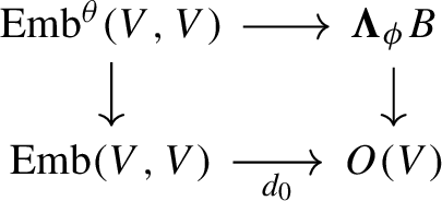
  Consequently, $\textrm{Emb}^{\theta }(V,V)\simeq {\varvec{\Lambda }}_{\phi } B$.

Proof

(1) We have $\textrm{Hom}_{\textrm{Top}_G^{\textrm{h}}/_{B}}(V,V)$ from Definition B.4 and showed in Proposition B.6 that restriction-to-the-base gives a natural G-equivalence:

$$\begin{aligned} \beta : \textrm{Hom}^{\theta }(\textrm{T}V, \textrm{T}V) \overset{\sim }{\rightarrow }\ \textrm{Hom}_{\textrm{Top}_G^{\textrm{h}}/_{B}}(V,V). \end{aligned}$$

Let $*$ be the G-space over B given by $\phi (0): * \rightarrow B$. We claim that the two maps $\textrm{inc}: 0 \rightarrow V$ and $\textrm{proj}: V \rightarrow *$ can be lifted to give equivalences of $V \simeq *$ in $\textrm{Top}_G^{\textrm{h}}/_{B}$. If so, pre-composing with $\textrm{inc}$ and post-composing with $\textrm{proj}$ give

$$\begin{aligned} \textrm{Hom}_{\textrm{Top}_G^{\textrm{h}}/_{B}}(V,V) \overset{\sim }{ \rightarrow } \textrm{Hom}_{\textrm{Top}_G^{\textrm{h}}/_{B}}(*, *) \cong {\varvec{\Lambda }}_{\phi } B. \end{aligned}$$

It remains to verify the claim, which is a routine job. We choose the lifts of $\textrm{inc}$ and $\textrm{proj}$ given by

$$\begin{aligned} I= & {} (\textrm{inc}, \alpha _1, 0) \in \textrm{Hom}_{\textrm{Top}_G^{\textrm{h}}/_{B}}(*,V), \text { where }\alpha _1(t) = \phi (0) \text { for all } t \ge 0.\\ P= & {} (\textrm{proj}, \alpha _2, 1) \in \textrm{Hom}_{\textrm{Top}_G^{\textrm{h}}/_{B}}(V,*), \text { where } \alpha _2(t) = {\left\{ \begin{array}{ll} \phi \circ h_t, &{} 0 \le t < 1; \\ \phi (0), &{} t \ge 1; \end{array}\right. } \end{aligned}$$

where $h_t:V \rightarrow V$ is any chosen homotopy from $h_0 = \textrm{id}$ to $h_1 = \textrm{proj}$. Then we have an obvious homotopy:

$$\begin{aligned} P \circ I = (\textrm{id}, \textrm{const}_{\phi (0)}, 1) \simeq (\textrm{id}, \textrm{const}_{\phi (0)}, 0) = \textrm{id}_{*} \end{aligned}$$

and using the contraction $h_t$, we can also construct a homotopy:

$$\begin{aligned} I \circ P = (\textrm{proj}, \alpha _2, 1) \simeq (\textrm{id}, \textrm{const}_{\phi }, 0) = \textrm{id}_{V}. \end{aligned}$$

(2) This is an assembly of part (1), Proposition B.11 and Theorem 2.24. However, we note that the map ${\varvec{\Lambda }}_{\phi }B \rightarrow O(V)$ is only a non-canonical G-equivalence. The author does not know how to upgrade it to a map of G-monoids. So although all spaces displayed in the pullback diagram are G-monoids, it is not obvious whether one can write $\textrm{Emb}^{\theta }(V,V)$ as a pullback of G-monoids.

To be more precise, we show how the quoted results assemble. We have the following large commutative diagram (B.16) expanding (B.13). Note that this is a commutative diagram of G-monoids.

The map $\varrho$ is studied in Lemma B.9. The map $\beta$ and the square $\textcircled {1}$ are in Proposition B.6. The diagonal unlabeled maps are all induced by the inclusion $V \rightarrow \textrm{T}V$ and the projection $\textrm{T}V \rightarrow V$. In particularly, the parallelogram $\textcircled {2}$ is in part (1). Naturality of $\varrho$ and $\beta$ gives the commutativity of $\textcircled {3}$ and $\textcircled {4}$. Now, $d_0$ in the theorem is the composite

and $d_0$ is an equivalence by taking $k=1$ and $M=V$ in Proposition 3.26. It can be seen that the vertical map in the theorem involves choosing an inverse of the $\beta$ displayed in the third line. $\square$

Remark B.17

The equivalence Theorem 2.24 is hidden in the following part of (B.16):

(See also [40, 4.4.12, 5.3.4].).

References

Ayala, D., Francis, J.: Factorization homology of topological manifolds. J. Topol. 8(4), 1045–1084 (2015)
Ayala, D., Mazel-Gee, A., Rozenblyum, N.: The geometry of the cyclotomic trace. arXiv preprint arXiv:1710.06409 (2017)
Andrade, R.: From manifolds to invariants of \(E_n\)-algebras. PhD thesis, Massachusetts Institute of Technology (2010)
Beilinson, A., Drinfeld, V.: Chiral Algebras. American Mathematical Society Colloquium Publications, vol. 51. American Mathematical Society, Providence, RI (2004)
Bödigheimer, C.F., Madsen, I.: Homotopy quotients of mapping spaces and their stable splitting. Quart. J. Math. Oxford 39, 401–409 (1988)
Berger, C., Moerdijk, I.: Axiomatic homotopy theory for operads. Comment. Math. Helv. 78(4), 805–831 (2003)
Ben-Zvi, D., Brochier, A., Jordan, D.: Integrating quantum groups over surfaces. J. Topol. 11(4), 874–917 (2018)
Costello, K., Gwilliam, O.: Factorization Algebras in Quantum Field Theory, vol. 1. Cambridge University Press, Cambridge (2016)
Cohen, F.R., Taylor, L.R.: Homology of function spaces. Math. Z. 198(3), 299–316 (1988)
Costenoble, S.R., Waner, S.: Fixed set systems of equivariant infinite loop spaces. Trans. Am. Math. Soc. 326(2), 485–505 (1991)
Dold, A., Thom, R.: Quasifaserungen und unendliche symmetrische Produkte. Ann. Math. 2(67), 239–281 (1958)
Galatius, S., Kupers, A., Randal-Williams, O.: Cellular \(E_k\)-algebras (2021)
Guillou, B., May, P.: Equivariant iterated loop space theory and permutative \(G\)-categories. Algebr. Geom. Topol. 17(6), 3259–3339 (2017)
Hahn, J., Horev, A., Klang, I., Wilson, D., Zou, F.: Equivariant Nonabelian Poincaré Duality and Equivariant Factorization Homology of Thom Spectra. arXiv preprint arxiv:2006.13348 (2020)
Horel, G.: Factorization homology and calculus à la Kontsevich Soibelman. J. Noncommut. Geom. 11(2), 703–740 (2017)
Horev, A.: Genuine Equivariant Factorization Homology. arXiv preprint arXiv:1910.07226 (2019)
Illman, S.: Smooth equivariant triangulations of \(G\)-manifolds for \(G\) a finite group. Math. Ann. 233(3), 199–220 (1978)
Kelly, G.M.: On the operads of J.P. May. Repr. Theory Appl. Categ. 13(1), (2005)
Kupers, A., Miller, J.: \(E_n\)-cell attachments and a local-to-global principle for homological stability. Math. Ann. 370(1–2), 209–269 (2018)
Kong, H., May, P., Zou, F.: Group completions and the homotopical monadicity theorem (2023) (preparation)
Knudsen, B.: Higher enveloping algebras. Geom. Topol. 22(7), 4013–4066 (2018)
Lashof, R.K.: Equivariant bundles. Illinois J. Math. 26(2), 257–271 (1982)
Lashof, R.K., May, J.P.: Generalized equivariant bundles. Bull. Soc. Math. Belg. Sér. A 38, 265–271 (1986)
Lewis, L.G., Jr., May, J.P., Steinberger, M., McClure, J.E.: Equivariant Sstable Homotopy Theory, volume 1213 of Lecture Notes in Mathematics, vol. 1213. Springer, Berlin (1986). (With contributions by J. E. McClure)
Lurie, J.: Higher algebra. http://www.math.harvard.edu/~lurie/papers/HA.pdf
May, J.P.: The geometry of iterated loop spaces. Springer, Berlin (1972). (Lectures Notes in Mathematics, Vol. 271)
May, J.P.: Classifying spaces and fibrations. Mem. Am. Math. Soc. 1 155(1, 155), xiii+98 (1975)
May, J.P.: Equivariant homotopy and cohomology theory, volume 91 of CBMS Regional Conference Series in Mathematics. Published for the Conference Board of the Mathematical Sciences, Washington, DC; by the American Mathematical Society, Providence, RI, (1996). With contributions by M. Cole, G. Comezaña, S. Costenoble, A. D. Elmendorf, J. P. C. Greenlees, L. G. Lewis, Jr., R. J. Piacenza, G. Triantafillou, and S. Waner
May, J.P.: Definitions: operads, algebras and modules. Contemporary Math. 202, 1–8 (1997)
McDuff, D.: Configuration spaces of positive and negative particles. Topology 14(1), 91–107 (1975)
Miller, J.: Nonabelian Poincaré duality after stabilizing. Trans. Am. Math. Soc. 367(3), 1969–1991 (2015)
May, J.P., Merling, M., Osorno, A.M.: Equivariant infinite loop space theory. The space level story. Mem. Am. Math. Soc. (2023) (to appear)
Manthorpe, R., Tillmann, U.: Tubular configurations: equivariant scanning and splitting. J. Lond. Math. Soc. 90(3), 940–962 (2014)
May, P., Zhang, R., Zou, F.: Operads, Monoids, Monads, and Bar Constructions. arXiv preprint arxiv:2003.10934 (2020)
Rourke, C., Sanderson, B.: Equivariant configuration spaces. J. Lond. Math. Soc. 62(2), 544–552 (2000)
Salvatore, Paolo: Configuration spaces with summable labels. In: Cohomological methods in homotopy theory (Bellaterra, 1998), volume 196 of Progr. Math., pp. 375–395. Birkhäuser, Basel (2001)
Steiner, R.: A canonical operad pair. Math. Proc. Cambridge Philos. Soc. 86(3), 443–449 (1979)
Salvatore, P., Wahl, N.: Framed discs operads and Batalin-Vilkovisky algebras. Q. J. Math. 54(2), 213–231 (2003)
Weelinck, T.A.N.: Equivariant factorization homology of global quotient orbifolds. Adv. Math. 366, 107072, 72 (2020)
Zou, F.: A Geometric Approach to Equivariant Factorization Homology and Nonabelian Poincaré Duality. PhD thesis, University of Chicago (2020)
Zou, F.: Notes on equivariant bundles. Expo. Math. 39(4), 644–678 (2021)
Acknowledgements
This paper is mostly based on my thesis. I would like to express my deepest gratitude to my advisor Peter May, who raises me up from the kindergarten of mathematics. I am indebted to Inbar Klang, Alexander Kupers and Jeremy Miller, whose work motivates my research. I would like to thank Asaf Horev and Haynes Miller for helpful conversations, Shmuel Weinberger for being my committee member, and the referees for making useful comments and catching small mistakes.
Author information
Authors and Affiliations
Corresponding author
Additional information
Publisher's Note
Springer Nature remains neutral with regard to jurisdictional claims in published maps and institutional affiliations.