Gradient regularity in mixed local and nonlocal problems

Abstract

Minimizers of functionals of the type

$$\begin{aligned} w\mapsto \int _{\Omega }[|Dw|^{p}-fw]\,\textrm{d}x+\int _{{\mathbb {R}}^{n}}\int _{{\mathbb {R}}^{n}}\frac{|w(x)-w(y)|^{\gamma }}{|x-y|^{n+s\gamma }}\,\textrm{d}x\,\textrm{d}y\end{aligned}$$

with $p, \gamma>1>s >0$ and $p> s\gamma$, are locally $C^{1, \alpha }$-regular in $\Omega$ and globally Hölder continuous.

1 Introduction

Mixed local and nonlocal problems are a subject of recent, emerging interest and intensive investigation. Essentially, the main object in question is an elliptic operator that combines two different orders of differentiation, the simplest model case being $-\Delta + (-\Delta )^{s}$, for $s \in (0,1)$. Here, the simultaneous presence of a leading local operator, and a lower order fractional one, constitutes the essence of the matter. In this special case, from a variational viewpoint, one is considering energies of the type

$$\begin{aligned} w\mapsto \int _{\Omega }|Dw|^{2}\,\textrm{d}x+\int _{{\mathbb {R}}^{n}}\int _{{\mathbb {R}}^{n}}\frac{|w(x)-w(y)|^{2}}{|x-y|^{n+2s}}\,\textrm{d}x\,\textrm{d}y\,, \qquad 0< s < 1\,. \end{aligned}$$

Here, as in all the rest of the paper, $\Omega \subset {\mathbb {R}}^n$ denotes at a bounded, Lipschitz regular domain and $n\ge 2$. First results in this direction have been obtained in [22,23,24, 44], via probabilistic methods; viscosity methods were pioneered in [3]. More recently, in a series of interesting papers, Biagi, Dipierro, Valdinoci, and Vecchi [6,7,8,9, 38] started a systematic investigation of problems involving mixed operators, proving a number of results concerning regularity and qualitative behaviour for solutions, maximum principles, and related variational principles. Up to now, the literature is mainly devoted to the study of linear operators. As for nonlinear cases, for instance those arising from functionals as

$$\begin{aligned} w\mapsto \int _{\Omega }[|Dw|^{p}-fw]\,\textrm{d}x+\int _{{\mathbb {R}}^{n}}\int _{{\mathbb {R}}^{n}}\frac{|w(x)-w(y)|^{\gamma }}{|x-y|^{n+s\gamma }}\,\textrm{d}x\,\textrm{d}y\,, \end{aligned}$$

(1.1)

the study of regularity of solutions has been confined to $L^\infty _{{\text {loc}}}(\Omega )$ and $C^{0, \alpha }_{{\text {loc}}}(\Omega )$ estimates (for small $\alpha$), that is, the classical De Giorgi–Nash–Moser theory. In this paper, our aim is to propose a different approach, aimed at proving maximal regularity of solutions to variational mixed problems in nonlinear, possibly degenerate cases as in (1.1). Specifically, we are going to prove the local Hölder continuity of the gradient of minimizers. Moreover, we also provide the first boundary regularity results for solutions. A sample of our results is indeed

Theorem 1

Let $u \in W^{1,p}_0(\Omega )\cap W^{s,\gamma }({\mathbb {R}}^n)$ be a minimizer of (1.1), with $p, \gamma>1>s >0$ and $p> s\gamma$, and such that $u\equiv 0$ on ${\mathbb {R}}^n\setminus \Omega$. If $f \in L^d(\Omega )$ for some $d>n$, then Du is locally Hölder continuous in $\Omega$. If $\partial \Omega \in C^{1, \alpha _b}$ for some $\alpha _b \in (0,1)$ and $f \in L^n(\Omega )$, then $u \in C^{0, \alpha }({\mathbb {R}}^n)$ for every $\alpha <1$.

Considering the more familiar case of the sum of two p-Laplaceans, we have

Theorem 2

Let $u\in W^{1,p}_{{\text {loc}}}(\Omega )\cap W^{s, p}({\mathbb {R}}^n)$ be a solution to

$$\begin{aligned} -\Delta _p u+(-\Delta _p)^s u =f \end{aligned}$$

(1.2)

in $\Omega$, with $p>1> s >0$ and $f \in L^d_{{\text {loc}}}(\Omega )$ for some $d>n$. Then Du is locally Hölder continuous in $\Omega$.

Our approach is flexible and allows us to consider general functionals of the type

$$\begin{aligned} {\mathcal {F}}(w):=\int _{\Omega }\left[ F(Dw)-fw\right] \,\textrm{d}x+\int _{{\mathbb {R}}^{n}}\int _{{\mathbb {R}}^{n}}\Phi (w(x)-w(y))K(x,y)\,\textrm{d}x\,\textrm{d}y\nonumber \\ \end{aligned}$$

(1.3)

modelled on the one in (1.1), i.e. $F(Dw)\approx |Dw|^p$ in the $C^2$-sense, $\Phi (t)\approx t^{\gamma }$ in the $C^1$-sense and $K(x,y) \approx |x-y|^{-n-s\gamma }$. Notice that, although we specialize to the variational setting, the regularity estimates we are presenting here actually work for general mixed equations almost verbatim, as our analysis is essentially based on the use of the Euler–Lagrange equation of functionals as in (1.3); for this, see Sect. 1.2. For the correct notion of minimality, and the related functional setting, as well as for results in full generality, see Sect. 1.1. Theorem 1 achieves the maximal regularity of minima, namely, the local Hölder continuity of the gradient of minimizers in $\Omega$. This is the best possible result already in the purely local case given by the p-Laplacean equation $-\Delta _pu=0$, which is covered by Uraltseva–Uhlenbeck theory and related counterexamples [64, 68, 69, 77, 78]. In addition, the case $p\not = \gamma$ is here considered for the first time, thereby allowing a full mixing between local and nonlocal terms. In this respect, the central assumption is

$$\begin{aligned} p>s\gamma \,, \end{aligned}$$

(1.4)

that says, roughly speaking, that the fractional $W^{s, \gamma }$-capacity generated by the nonlocal term in (1.1) can be controlled by the $W^{1, p}$-capacity (the standard p-capacity) generated by $w \mapsto \int |Dw|^p\,\textrm{d}x$. This is exactly the point ensuring that the nonlocal term in (1.1) has less regularizing effects that the local one, as it happens in the basic case $-\Delta + (-\Delta )^{s}$, when $p=\gamma =2$, and also in the nonlinear models of the type $-\Delta _p+ (-\Delta _p)^s$, where the fractional p-Laplacean operator appears [27, 41, 42, 45, 55, 56, 59, 60]. We also Notice that, as far as we known, allowing the condition $p\not = \gamma$ is a new, non-trivial feature already when $p=2$ and that even the basic De Giorgi–Nash–Moser theory is not available when $p\not =\gamma$. As a matter of fact, all our estimates simplify in the case $p=\gamma$.

We have reported Theorem 1 for the sake of exposition but it is actually a very special case of more general results, i.e., Theorems 3–5, whose statements are necessarily more involved due to their greater generality. Before stating the precise assumptions and the results in full generality, we spend a few words about the techniques we are going to use, and on some relevant connections. Up to now, the methods proposed in the literature to deal with mixed operators are, in a sense, direct. More precisely, both the local terms and the nonlocal ones stemming from the equations interact simultaneously via energy methods. These techniques ultimately rely on those used in the nonlocal case [10,11,12, 35, 36, 55, 56, 59, 60] for purely nonlocal operators. This approach does not allow to prove regularity of solutions beyond that allowed by nonlocal operators techniques, which is not the best one can hope for, as, in mixed operators, the leading regularizing term is the local one. In this paper we reverse the approach, relying more on the methods, and, especially, on the estimates available in regularity theory of local operators. In a sense, we separate the local and nonlocal part combining energy estimates of Caccioppoli type with a perturbative like approach. The crucial point is to fit the terms stemming from the nonlocal term in the iteration procedures that would naturally come up from considering the local part only. For this we have to consider a complex scheme of quantities, interacting with each other, and controlling simultaneously both the oscillations of the solution on small balls, and those averaging the oscillations over their complement (such quantities are detailed in Sect. 3). This first leads to Hölder regularity of solutions with every exponent (Theorem 3) and then to the same kind of estimates globally (Theorem 4); combining these ingredients with a priori regularity estimates from the classical local theory, leads to Theorem 5. We mention that, due to the assumption $p\not =\gamma$, functionals as in (1.1)–(1.3) connect to a large family of problems featuring anisotropic operators and integrands with so-called nonstandard growth conditions [26, 28, 29, 32, 40, 54, 66], and to some other classes of anisotropic nonlocal problems [16,17,18,19,20, 33, 67, 73]. We mention that a further connection has been established in [31], where a class of mixed functionals has been used to approximate local functionals with (p, q)-growth in order to prove higher integrability of minimizers. Further approximations via mixed operators occur in the interesting paper [74].

1.1 Assumptions and results

When considering the functional ${\mathcal {F}}$ in (1.3), the integrand $F:{\mathbb {R}}^{n}\rightarrow {\mathbb {R}}$ is assumed to be $C^{2}({\mathbb {R}}^{n}\setminus \{0\})\cap C^{1}({\mathbb {R}}^{n})$-regular and to satisfy the following standard p-growth and coercivity assumptions (see [63, 68, 69])

$$\begin{aligned} {\left\{ \begin{array}{ll} \ \Lambda ^{-1}(|z|^{2}+\mu ^{2})^{p/2}\le F(z)\le \Lambda (|z|^{2}+\mu ^{2})^{p/2}\\ \ |\partial _{z} F(z)|+(|z|^{2}+\mu ^{2})^{1/2}|\partial _{zz}F(z)|\le \Lambda (|z|^{2}+\mu ^{2})^{(p-1)/2}\\ \ \Lambda ^{-1}(|z|^{2}+\mu ^{2})^{(p-2)/2}|\xi |^{2}\le \partial _{zz}F(z)\xi \cdot \xi \end{array}\right. } \end{aligned}$$

(1.5)

for all $z\in {\mathbb {R}}^{n}\setminus \{0\}$, $\xi \in {\mathbb {R}}^{n}$, where $\mu \in [0,1]$ and $\Lambda \ge 1$ are fixed constants. The function $\Phi :{\mathbb {R}}\rightarrow {\mathbb {R}}$ is assumed to satisfy

$$\begin{aligned} {\left\{ \begin{array}{ll} \ \Phi (\cdot )\in C^{1}({\mathbb {R}})\,, \quad t\mapsto \Phi (t) \ \text {is convex}\\ \ \Lambda ^{-1}|t|^{\gamma }\le \Phi (t)\le \Lambda |t|^{\gamma }\,, \quad \Lambda ^{-1}|t|^{\gamma }\le \Phi '(t)t\le \Lambda |t|^{\gamma } \end{array}\right. } \end{aligned}$$

(1.6)

for all $t\in {\mathbb {R}}$. The kernel $K:{\mathbb {R}}^n\times {\mathbb {R}}^n \rightarrow {\mathbb {R}}$ satisfies

$$\begin{aligned} \frac{\texttt {k} }{\Lambda |x-y|^{n+s\gamma }}\le K(x,y)\le \frac{\Lambda \texttt {k} }{|x-y|^{n+s\gamma }}, \qquad \text{ where } \texttt {k} \in (0,1] \end{aligned}$$

(1.7)

for all $x,y\in {\mathbb {R}}^n, x\not =y$. As already mentioned, unless otherwise stated, $p,s,\gamma$ are such that $p,\gamma>1>s >0$, with $p> s\gamma$. We shall consider a boundary datum $g\in W^{1,p}(\Omega )\cap W^{s,\gamma }({\mathbb {R}}^{n})$. In order to get global continuity of minimizers, we consider the following requirements on the boundary $\partial \Omega$:

$$\begin{aligned} {\left\{ \begin{array}{ll} \partial \Omega \in C^{1, \alpha _b},\ \ \alpha _b \in (0,1)\\ g\in W^{1,q}(\Omega )\cap W^{a,\chi }({\mathbb {R}}^{n})\\ q>p,\ \ a>s,\ \ \chi>\gamma , \ \ \kappa :=\min \{1-n/q, a-n/\chi \}>0\,. \end{array}\right. } \end{aligned}$$

(1.8)

In particular, this implies that we are assuming $q, a\chi >n$. Interior Hölder estimates, both for minima and their gradients, need less, and essentially no boundary assumptions; for this, we shall replace (1.8) by the weaker

$$\begin{aligned} g\in L^{\infty }({\mathbb {R}}^{n}) \end{aligned}$$

(1.9)

that in fact will only be needed in when $\gamma >p$. Note that $W^{a,\chi }({\mathbb {R}}^{n})\subset L^\infty ({\mathbb {R}}^n)$ holds provided $a-n/\chi >0$ [37, Theorem 8.2]. Conditions (1.5)–(1.9) lead to consider the following natural functional setting:

$$\begin{aligned} {\left\{ \begin{array}{ll} \ {\mathbb {X}}_{g}(\Omega ):=\left\{ w\in g + W^{1,p}_0(\Omega )\cap W^{s,\gamma }({\mathbb {R}}^{n}):w\equiv g \ \text{ in } \ \ {\mathbb {R}}^{n}\setminus \Omega \right\} \\ \ {\mathbb {X}}_{0}(\Omega ):=\left\{ w\in W^{1,p}_0(\Omega )\cap W^{s,\gamma }({\mathbb {R}}^{n}):w\equiv 0 \ \text{ in } \ {\mathbb {R}}^{n}\setminus \Omega \right\} \,. \end{array}\right. } \end{aligned}$$

Note that some ambiguity arises in the definition of ${\mathbb {X}}_{g}$; in fact, this is actually meant as the subspace of functions $w\in W^{s, \gamma }({\mathbb {R}}^n)$ whose restriction on $\Omega$ belongs to $g + W^{1,p}_0(\Omega )$. Compare for instance with the discussion made in [6, 9], where related functional settings are considered. Under assumptions (1.5)–(1.7) and (1.9), and $f \in W^{-1, p'}(\Omega )$ (the dual of $W^{1,p}_0(\Omega )$), there exists a unique solution $u\in {\mathbb {X}}_{g}(\Omega )$ to

$$\begin{aligned} {\mathbb {X}}_{g}(\Omega )\ni u\mapsto \min _{w \in {\mathbb {X}}_{g}(\Omega )} {\mathcal {F}}(w)\,. \end{aligned}$$

(1.10)

Moreover

$$\begin{aligned}&\int _{\Omega }\left[ \partial _{z} F(Du)\cdot D\varphi -f\varphi \right] \,\textrm{d}x\nonumber \\&\quad +\int _{{\mathbb {R}}^{n}}\int _{{\mathbb {R}}^{n}}\Phi '(u(x)-u(y))(\varphi (x)-\varphi (y)) K(x,y)\,\textrm{d}x\,\textrm{d}y=0 \end{aligned}$$

(1.11)

holds for every $\varphi \in {\mathbb {X}}_{0}(\Omega )$. The proof of these facts is quite standard, and relies on the application of Direct Methods of the Calculus of Variations. The details can be found for instance in [31, Sections 3.3–3.5], where actually a more delicate case of mixed operators is considered. As for the derivation of the Euler–Lagrange equation, this is standard once (1.5)–(1.7) are assumed, and, for the nonlocal part, proceeds as in [31, 35].

Theorem 3

(Almost Lipschitz local continuity) Under assumptions (1.5)–(1.7) and (1.9), with $f\in L^n(\Omega )$, let $u\in {\mathbb {X}}_{g}(\Omega )$ be as in (1.10). Then $u\in C^{0,\alpha }_{{\text {loc}}}(\Omega )$ for every $\alpha \in (0,1)$ and, for every open subset $\Omega _0\Subset \Omega$, $[u]_{0, \alpha ;\Omega _0} \le c$ holds with $c\equiv c(\texttt {data} _{\text {h}},\alpha , \,\textrm{dist}(\Omega _0, \partial \Omega ))$. Assumption (1.9) can be dropped when $\gamma \le p$.

Theorem 4

(Global Hölder continuity) Under assumptions (1.5)–(1.8) with $f\in L^n(\Omega )$, let $u\in {\mathbb {X}}_{g}(\Omega )$ be as in (1.10). Then $u\in C^{0,\alpha }({\mathbb {R}}^n)$ for every $\alpha < \kappa$ and $[u]_{0, \alpha ;{\mathbb {R}}^n}\le c (\texttt {data} )$. If, in addition, $g \in W^{1, \infty } ({\mathbb {R}}^n)$, then $u\in C^{0,\alpha }({\mathbb {R}}^n)$ for every $\alpha <1$.

Theorem 5

(Gradient local Hölder continuity) Under assumptions (1.5)–(1.7) and (1.9), with $f\in L^d(\Omega )$ for some $d>n$, let $u\in {\mathbb {X}}_{g}(\Omega )$ be as in (1.10). Then there exists $\alpha \equiv \alpha (n,p,s,\gamma , \Lambda ,d) \in (0,1)$, such that $Du\in C^{0,\alpha }_{{\text {loc}}}(\Omega ;{\mathbb {R}}^n)$ and, for every open subset $\Omega _0\Subset \Omega$, $[Du]_{0, \alpha ;\Omega _0} \le c$ holds with $c\equiv c(\texttt {data} _{\text {h}}, \Vert f\Vert _{L^d(\Omega )},\,\textrm{dist}(\Omega _0, \partial \Omega ))$. Assumption (1.9) can be dropped when $\gamma \le p$.

The (shorthand) notation concerning the dependence on the constants used in Theorems 3–5 is

$$\begin{aligned} {\left\{ \begin{array}{ll} \, \texttt {data} _{\text {h}}:=(n,p,s,\gamma ,\Lambda ,\Vert f\Vert _{L^n(\Omega )},\Vert u \Vert _{L^{p}(\Omega )},\Vert u \Vert _{L^{\gamma }({\mathbb {R}}^n)} ) \ \ \text{ if } \gamma \le p\\ \, \texttt {data} _{\text {h}}:=(n,p,s,\gamma ,\Lambda ,\Vert f\Vert _{L^n(\Omega )},\Vert u \Vert _{L^{\infty }(\Omega )},\Vert u \Vert _{L^{\gamma }({\mathbb {R}}^n)} ) \ \ \text{ if } \gamma > p\\ \, \texttt {data} :=(n,p,s,\gamma ,\Lambda ,\Vert f\Vert _{L^n(\Omega )},\Vert g \Vert _{W^{1,q}(\Omega )},\Vert g \Vert _{W^{s,\gamma }({\mathbb {R}}^n)},\Vert g \Vert _{W^{a,\chi }({\mathbb {R}}^n)},\Omega )\,. \end{array}\right. } \end{aligned}$$

(1.12)

Notice that none of the above lists contains the parameter $\texttt {k}$ appearing in (1.7). For the sake of brevity we shall sometimes indicate a dependence of a constant c on one of the lists in (1.12), also when it will actually occur on a subset of the parameters involved. For example, a constant c depending only on $n,p,s,\gamma$ might be still indicated as $c \equiv c (\texttt {data} _{\text {h}})$.

Remark 1

Le us briefly comment on the previous results.

• Theorem 3 is sharp in the sense it does not hold when only assuming that $f \in L^t$, for any $t<n$. As for Theorem 5, one cannot obtain in general the gradient Hölder continuity only assuming that $f\in L^n$; counterexamples arise already in the purely local (and linear) case $-\Delta u=f$ [25]. See Theorem 7 below for more in this direction and Sect. 8.1.

• All the a priori estimates in this paper are independent of the constant $\texttt {k} \in (0,1]$ appearing in (1.7). In particular, everything remains stable when $\texttt {k} \rightarrow 0$. In this case the equations covered are of the type $-\Delta _p u+ \texttt {k} (-\Delta _\gamma )^s u =f,$ for which the corresponding estimates are uniform with respect to $\texttt {k} \in (0,1]$. This is natural in view of our perturbative approach (we thank the referee for pointing out this aspect to us).

• When considering the case $\gamma \le p$, in Theorems 3 and 5 no assumption is put on the boundary datum g, and, in fact, our results can be formulated in a purely local fashion. See Remark 3 and Theorem 6 below. Note that, in the case $\gamma \le p$, on the contrary of other papers devoted to the subject, we dot not need to prove that u is bounded to get its Hölder continuity. This is typical in the regularity theory of the local operators when using perturbative methods.

• As far as we know, Theorem 4 is the first boundary regularity appearing in the literature for the class of nonlinear problems considered here. Assumptions as (1.8), implying that $g\in C^{0, \kappa }({\mathbb {R}}^n)$ via higher gradient integrability, are quite common in the boundary regularity of local problems; see for instance [21, 39] and [48, Section 7.8]. We further comment on this in Sect. 8 and refer to [43, 51, 52, 75] for boundary regularity results in the purely nonlocal case, where it is $g\equiv 0$.

• A general remark concerning the results in this paper. As our approach is ultimately perturbative, our results and the form of the a priori estimates obtained should not be directly compared to those available for the $(-\Delta _\gamma )^s$-Laplacean operator (as for instance those in [35, 36]), but rather with those available in the regularity theory of the classical p-Laplacean operator. Anyway, the functional setting we adopt in Theorems 4-8, featuring the space ${\mathbb {X}}_{g}$, is in line with some of those typically used in the setting of nonlocal problems, see for instance [35, 36]. In order to keep the emphasis on the main points, i.e., on a priori estimates, we prefer the basic setting adopted here, just using natural energy spaces (see for instance [11, 72] for related Tail spaces in the purely nonlocal setting and the comments at the end of Remark 3). Further comments on this point are in Sect. 7. A interesting local approach, with local solutions, can be found in [46] (see also the comments at the end of Sect. 1.2).

1.2 Possible extensions

Several extensions are possible. For instance, one can consider more general functionals of the type

$$\begin{aligned} w \mapsto \int _{\Omega }\left[ F(x,Dw)-fw\right] \,\textrm{d}x+\int _{{\mathbb {R}}^{n}}\int _{{\mathbb {R}}^{n}}\Phi (w(x)-w(y))K(x,y)\,\textrm{d}x\,\textrm{d}y\,, \end{aligned}$$

where this time we assume that $z \mapsto F(x, z)$ satisfies (1.5) uniformly with respect to $x\in \Omega$. The assumption regulating coefficients is

$$\begin{aligned} |\partial _z F(x,z)-\partial _z F(y, z)| \le \Lambda \omega (|x-y|)(|z|^{2}+\mu ^{2})^{(p-1)/2}\,, \end{aligned}$$

(1.13)

to hold for every choice $x, y \in \Omega$ and $z \in {\mathbb {R}}^n$. Here $\omega :[0, \infty ) \rightarrow [0, 1)$ is a modulus of continuity, that is, a continuous and non-decreasing function, such that $\omega (0)=0$. Under assumption (1.13), it is then easy to see that Theorems 3 and 4 continue to hold. In order to get an analog of Theorem 5 we assume in addition that $\omega (t) \le t^{\sigma }$ holds for some $\sigma \in (0,1)$, this condition being necessary; then the Hölder exponent of Du does not exceed $\sigma$. We note the proof of these assertions is in fact implicit in the proof of boundary regularity provided in Proposition 5.1 below.

Another extension, already mentioned above, is about general solutions to nonlinear mixed integroredifferential operators, not necessarily coming from integral functionals. Moreover, a purely local regularity approach can be considered. For this, we consider a general vector field $A :{\mathbb {R}}^n\rightarrow {\mathbb {R}}^n$ such that $A \in C^{0}({\mathbb {R}}^n)\cap C^1({\mathbb {R}}^n\setminus \{0\})$, and a functions $\Psi \in C^{0}({\mathbb {R}})$, f such that

$$\begin{aligned} {\left\{ \begin{array}{ll} \ | A(z)|+(|z|^{2}+\mu ^{2})^{1/2}|\partial _{z}A(z)|\le \Lambda (|z|^{2}+\mu ^{2})^{(p-1)/2}\\ \ \Lambda ^{-1}(|z|^{2}+\mu ^{2})^{(p-2)/2}|\xi |^{2}\le \partial _{z}A(z)\xi \cdot \xi \\ \ \Lambda ^{-1}|t|^{\gamma }\le \Psi (t)t\le \Lambda |t|^{\gamma },\qquad f \in W^{-1, p'}(\Omega )\,, \end{array}\right. } \quad \end{aligned}$$

(1.14)

with the same meaning of (1.5) and (1.6). Note that the classical p-Laplacean operator given by $A(z)\equiv |z|^{p-2}z$ is covered by (1.14). We consider functions $u\in W^{1,p}(\Omega )\cap W^{s, \gamma }({\mathbb {R}}^n)$, where $\Omega \subset {\mathbb {R}}^n$ is as usual a bounded and Lipschitz-regular domain, such that

$$\begin{aligned}&\int _{\Omega }\left[ A(Du)\cdot D\varphi -f\varphi \right] \,\textrm{d}x\nonumber \\&\quad +\int _{{\mathbb {R}}^{n}}\int _{{\mathbb {R}}^{n}}\Psi (u(x)-u(y))(\varphi (x)-\varphi (y)) K(x,y)\,\textrm{d}x\,\textrm{d}y=0 \end{aligned}$$

(1.15)

holds for every $\varphi \in {\mathbb {X}}_{0}(\Omega )$ (see also Sect. 7). Notice that here no boundary datum g appears and the definition of solution is instead local; we expand on this in Sect. 7. In this case we have

Theorem 6

Under assumptions (1.7) and (1.14), let $u\in W^{1,p}(\Omega )\cap W^{s, \gamma }({\mathbb {R}}^n)$ be a solution to (1.15).

• If $u \in L^{\infty }_{{\text {loc}}}(\Omega )$ when $\gamma >p$, and $f \in L^n_{{\text {loc}}}(\Omega )$, then $u\in C^{0,\alpha }_{{\text {loc}}}(\Omega )$ for every $\alpha \in (0,1)$.

• If $u \in {\mathbb {X}}_{g}(\Omega )$, $f \in L^n(\Omega )$ and conditions (1.8) hold, then $u \in C^{0,\alpha }({\mathbb {R}}^n)$ for every $\alpha < \kappa$.

• If $u \in L^{\infty }_{{\text {loc}}}(\Omega )$ when $\gamma >p$, and $f \in L^d_{{\text {loc}}}(\Omega )$ for some $d>n$, then $u\in C^{1,\alpha }_{{\text {loc}}}(\Omega )$ for some $\alpha \in (0,1)$.

The proof of Theorem 6 follows verbatim the ones for Theorems 3–5 taking into account the content of Remark 3 and Sect. 7. Again, notice that the assumption $u \in L^\infty _{{\text {loc}}}$ is only needed when $\gamma > p$. Notice also that Theorem 2 is a special case of Theorem 6.

The methods developed in this paper also yield intermediate Hölder regularity results. We confine ourselves to give a sample of this in the interior case. Similar estimates should also hold globally. The following version of Theorem 3 responds to a question posed by the referee of a first version of the manuscript.

Theorem 7

(Quantified Hölder continuity) Under assumptions (1.5)–(1.7) and (1.9), if $u\in {\mathbb {X}}_{g}(\Omega )$ is as in (1.10) and $f \in L^q(\Omega )$, then

$$\begin{aligned} {\left\{ \begin{array}{ll} p\le n \text{ and } q=\frac{n}{p-\alpha (p-1)}, \, \alpha \in (0,1) \\ p> n\text{, } q=1 \text{ and } \alpha = \frac{p-n}{p-1} \end{array}\right. } \Longrightarrow u\in C^{0,\alpha }_{{\text {loc}}}(\Omega ). \end{aligned}$$

(1.16)

Assumption (1.9) can be dropped when $\gamma \le p$.

As expected by the methods we employ, Theorem 7 reproduces, in terms of the integrability assumptions on f, the same Hölder local regularity results that hold in the local case $-\Delta _pu=f$; see [58, Corollary 1] and Sect. 8.1. Note that when $p>n$ solutions are automatically $\alpha$-Hölder continuous with exponent $\alpha = 1-n/p$ by Sobolev–Morrey embedding. This is smaller that the one appearing in (1.16). Accordingly, a priori estimates come along:

Theorem 8

(Campanato type estimate for Theorems 3 and 7) Under the assumptions and the notation of Theorem 7. There exist $r_*>0$ and $c\ge 1$ such that

(1.17)

holds whenever $B_{\varrho }\equiv B_{\varrho }(x_0)\subset B_{r}(x_0)\equiv B_{r} \subset \Omega _0$ are concentric balls with $r\le r_*\in (0,1)$ and for $\delta \in ( s\gamma ,p)$ sufficiently close to p. Both $r_*$ and c depend on $n,p,s,\gamma ,\Lambda , \alpha$ if $\gamma \le p$, and also on $\Vert u\Vert _{L^\infty (\Omega )}$ when $\gamma >p$. Assumption (1.9) can be dropped when $\gamma \le p$.

When $\gamma \le p$ the constant c in (1.17) only depends on $n,p,s,\gamma ,\Lambda$. Dropping the terms containing $\,\textrm{d}\lambda _{x_0}$ arising from the nonlocal part, (1.17) gives back the classical Campanato type decay estimate for solutions to local non-homogeneous equations (see for instance [48, Theorem 7.7] or [58]). Estimate (1.17) implies the local $C^{0, \alpha }$-regularity of solutions, with related a priori estimates. An additional feature of estimate (1.17) is a power decay of the term

which is a manipulation of a quantity called $\texttt {snail}$, that is of common use in nonlocal problems (see Sect. 3 for more). In the range $\gamma >p$, the nonlocal term exhibits a growth larger than the local one, and a careful analysis of the proofs, actually reveals that the constant c appearing in (1.17), depends on $n,p,s, \gamma , \Lambda$ and locally on $\Vert u\Vert _{L^\infty }$ (see Remark 3 for details). This typically happens in all those local situations when anisotropic operators are considered, especially in the setting of nonuniformly elliptic problems (see for instance the a priori estimates in [26, 29, 31, 32]).

We finally remark that, after a first draft of this paper was poster on the Arxiv¹ and submitted, a related, interesting preprint of Garain and Lindgren [46] appeared, where results connected to ours are contained for a different range of parameters (in particular, in [46] it is $\gamma =p$) and starting by a slightly weaker notion of solutions. The techniques in [46] are completely different from those employed here.

2 Preliminaries

2.1 Notation

Unless otherwise specified, we denote by c a general constant larger or equal than 1. Different occurrences from line to line will be still denoted by c. Special occurrences will be denoted by $c_*, c_1$ or likewise. Relevant dependencies on parameters will be as usual emphasized by putting them in parentheses. In the following, given $a\in {\mathbb {R}}$, we denote $a_+:=\max \{a,0\}$. We denote by $B_r(x_0):= \{x \in {\mathbb {R}}^n : |x-x_0|< r\}$ the open ball with center $x_0$ and radius $r>0$; we omit denoting the center when it is not necessary, i.e., $B \equiv B_r \equiv B_r(x_0)$; this especially happens when various balls in the same context share the same center. With $B_{r}^{+}(x_{0})$ we mean the upper half ball $B_{r}(x_{0})\cap \left\{ x\in {\mathbb {R}}^{n}:x_{n}>0 \right\}$; in connection, we denote $\Gamma _{r}(x_{0}):=B_{r}(x_0)\cap \{x_n=0\}$, whenever $x_0 \in \{x_n=0\}$. With ${\mathcal {B}} \subset {\mathbb {R}}^{n}$ being a measurable subset with respect to a Borel (non-negative) measure $\lambda _0$ in ${\mathbb {R}}^n$, with bounded positive measure $0<\lambda _0({\mathcal {B}})<\infty$, and with $b :{\mathcal {B}} \rightarrow {\mathbb {R}}^{k}$, $k\ge 1$, being a measurable map, we denote

According to the standard notation, given $b :{\mathcal {B}} \rightarrow {\mathbb {R}}^k$, we denote

$$\begin{aligned}{}[b]_{0,\alpha ;\, {\mathcal {B}}}:= \sup _{x,y\in {\mathcal {B}}; x\not = y}\, \frac{|b(x)-b(y)|}{|x-y|^\alpha }\,, \qquad \mathop {{{\,\textrm{osc}\,}}}\limits _{{\mathcal {B}}} b := \sup _{x, y \in {\mathcal {B}}} \, |b(x)-b(y)| \end{aligned}$$

for $0< \alpha \le 1$ and ${\mathcal {B}} \subset {\mathbb {R}}^{n}$ being a set.

2.2 Fractional spaces

For $\gamma \ge 1$ and $s\in (0,1)$, the space $W^{s,\gamma }({\mathbb {R}}^{n})$ is defined via

$$\begin{aligned} W^{s,\gamma }({\mathbb {R}}^{n}):=\left\{ w\in L^{\gamma }({\mathbb {R}}^{n}):\int _{{\mathbb {R}}^{n}}\int _{{\mathbb {R}}^{n}}\frac{|w(x)-w(y)|^{\gamma }}{|x-y|^{n+s\gamma }}\,\textrm{d}x\,\textrm{d}y<\infty \right\} , \end{aligned}$$

and it is endowed with the norm

$$\begin{aligned} \Vert w \Vert _{W^{s,\gamma }({\mathbb {R}}^{n})}:=\left( \int _{{\mathbb {R}}^{n}}|w|^{\gamma }\,\textrm{d}x\right) ^{1/\gamma }+\left( \int _{{\mathbb {R}}^{n}}\int _{{\mathbb {R}}^{n}}\frac{|w(x)-w(y)|^{\gamma }}{|x-y|^{n+s\gamma }}\,\textrm{d}x\,\textrm{d}y\right) ^{1/\gamma }\,. \end{aligned}$$

With $w\in W^{s,\gamma }({\mathbb {R}}^{n})$, we also denote

$$\begin{aligned}{}[w]_{s,\gamma ;A}:= \left( \int _{A}\int _{A}\frac{|w(x)-w(y)|^{\gamma }}{|x-y|^{n+s\gamma }}\,\textrm{d}x\,\textrm{d}y\right) ^{1/\gamma } \end{aligned}$$

whenever $A \subset {\mathbb {R}}^n$ is measurable. In a similar way, by replacing ${\mathbb {R}}^n$ by $\Omega$ in the domain of integration, it is possible to define the fractional Sobolev space $W^{s,\gamma }(\Omega )$ in an open domain $\Omega \subset {\mathbb {R}}^{n}$. Good general references for fractional Sobolev spaces are [1, 37]. For the next result, see also [2] and related references.

Lemma 2.1

(Fractional Poincaré) Let $\gamma \in [1, \infty )$, $s\in (0,1)$, $B_{\varrho }\subset {\mathbb {R}}^{n}$ be a ball. If $w\in W^{s,\gamma }(B_{\varrho })$, then

(2.1)

holds with $c\equiv c(n,s,\gamma )$.

Lemma 2.2

(Embedding) Let $1\le \gamma \le p<\infty$, $s\in (0,1)$ and $B_{\varrho } \subset {\mathbb {R}}^{n}$ be a ball. If $w\in W^{1,p}_{0}(B_{\varrho })$, then $w\in W^{s,\gamma }(B_{\varrho })$ and

holds with $c\equiv c(n,p,s,\gamma )$

Proof

By standard rescaling—i.e., passing to $B_1\ni x\mapsto w(x_{0}+\varrho x)$, with $x_0$ being the center of $B_{\varrho }$—we can reduce to the case $B_{\varrho }\equiv B_1(0)$. The assertion then follows by [37, Proposition 2.2] and standard Poincaré’s inequality, as $w\in W^{1,p}_{0}(B_{1})$. $\square$

Using interpolation from [14] (see also [13]), we can also prove the following improved imbedding:

Lemma 2.3

(Localized interpolation) Let $1<p < \gamma \le p/s$ and $s\in (0,1)$, $B_{\varrho }\subset {\mathbb {R}}^{n}$. If $w\in W^{1,p}_{0}(B_{\varrho })\cap L^{\infty }(B_{\varrho })$, then $w\in W^{s,\gamma }(B_{\varrho })$ and

(2.2)

holds with $c\equiv c(n,p,s,\gamma )$.

Proof

Note that, on the contrary to the rest of the paper, here we are allowing $p=s\gamma$; this is not really needed in what follows, but we include this case for completeness. Again we can assume that $B_{\varrho }(x_{0})\equiv B_1(0)$, and, letting $w\equiv 0$ outside $B_1(0)$, we can assume $w\in W^{1,p}_{0}({\mathbb {R}}^n)\cap L^{\infty }({\mathbb {R}}^n)$. We first consider the case $p>s\gamma$. We shall use the off-diagonal interpolation results from [14] in Triebel–Lizorkin spaces $F^{\sigma }_{\lambda , t}$ [76, 2.3.1]. Specifically, we use the following interpolation inequality, that holds whenever $0\le \sigma _{1}<\sigma _{2}<\infty$ and $\lambda _{1},\lambda _{2}\in (1,\infty )$ and $t, t_1, t_2\ge 1$

$$\begin{aligned} \Vert w \Vert _{F^{\sigma }_{\lambda , t}({\mathbb {R}}^{n})}\le c\Vert w \Vert _{F^{\sigma _1}_{\lambda _1, t_1}({\mathbb {R}}^{n})}^{\theta }\Vert w \Vert _{F^{\sigma _2}_{\lambda _2, t_2}({\mathbb {R}}^{n})}^{1-\theta }\,, \end{aligned}$$

(2.3)

provided $\theta \in (0,1)$ is such that $\sigma =\theta \sigma _{1}+(1-\theta )\sigma _{2}$ and $1/\lambda =\theta /\lambda _{1}+(1-\theta )/\lambda _{2}$, where $c\equiv c(n,\sigma _{i},\lambda _{i},t_{i},\theta )$; see [14, Lemma 3.1]. Note the off-diagonal character of (2.3), that lies in the fact that $t,t_1,t_2$ can be chosen arbitrarily. From [14, Pag. 390] and [15, Proposition 5.3] we recall the identities $F^{0}_{\lambda _1,2}({\mathbb {R}}^{n})\equiv L^{\lambda _1}({\mathbb {R}}^{n})$, $F^{1}_{\lambda _2,2}({\mathbb {R}}^{n})\equiv W^{1,\lambda _2}({\mathbb {R}}^{n})$ and $F^{\sigma }_{\lambda ,\lambda }({\mathbb {R}}^{n})\equiv W^{\sigma ,\lambda }({\mathbb {R}}^{n})$ when $\sigma \in (0,1)$. This means that (2.3) turns into

$$\begin{aligned} \Vert w \Vert _{W^{\sigma ,\lambda }({\mathbb {R}}^{n})}\le c\Vert w \Vert _{L^{\lambda _1}({\mathbb {R}}^{n})}^{1-\sigma }\Vert w \Vert _{W^{1,\lambda _2}({\mathbb {R}}^{n})}^{\sigma }\,, \end{aligned}$$

(2.4)

with $\sigma \in (0,1)$ and $1/\lambda =(1-\sigma )/\lambda _{1}+\sigma /\lambda _{2}$; see also [15]. Now, observe that $1<p< \gamma$ and $p>s\gamma$ imply $(1-s)\gamma p/(p-s\gamma )>1,$ therefore in (2.4), we can take $\lambda _{1}=(1-s)\gamma p/(p-s\gamma )$, $\sigma =s$ and $\lambda _{2}=p$; via Poincaré’s inequality this yields

$$\begin{aligned}{}[w]_{s,\gamma ;B_1} \le c\Vert w \Vert _{L^{\lambda _{1}}(B_1)}^{1-s}\Vert w \Vert ^{s}_{W^{1,p}(B_1)} \le c\Vert w \Vert _{L^{\infty }(B_1)}^{1-s}\Vert Dw \Vert ^{s}_{L^{p}(B_1)}, \end{aligned}$$

with $c\equiv c(n,p,s,\gamma )$, that is (2.2) when $s\gamma <p$. On the other hand, if $s\gamma =p$, we use [14, Corollary 3.2, (c)], that is $[w]_{\theta \sigma ,\lambda /\theta ;{\mathbb {R}}^{n}}\le c\Vert w \Vert _{L^{\infty }({\mathbb {R}}^{n})}^{1-\theta }\Vert w \Vert _{W^{\sigma ,\lambda }({\mathbb {R}}^{n})}^{\theta }$, that holds whenever $\theta \in (0,1)$, where $c\equiv c(n,\sigma ,\lambda ,\theta )$. We use this with $\sigma =1$, $\lambda =p$, $\theta =s$ and get

$$\begin{aligned}{}[w]_{s,p/s;B_1}\le c\Vert w \Vert _{L^{\infty }(B_1)}^{1-s}\Vert w \Vert _{W^{1,p}(B_1)}^{s} \le c\Vert w \Vert _{L^{\infty }(B_1)}^{1-s}\Vert Dw \Vert _{L^{p}(B_1)}^{s}, \end{aligned}$$

with $c\equiv c(n,p,s)$, and the proof is complete. $\square$

We find it useful to have a unified reformulation of Lemmas 2.2-2.3. For this, we introduce, with reference to the exponents $p, s, \gamma$ considered in Theorems 1-5, the following quantities:

$$\begin{aligned} \vartheta :={\left\{ \begin{array}{ll} \ s\quad &{}\text{ if } \ \ \gamma>p\\ \ 1\quad &{}\text{ if } \ \ \gamma \le p \end{array}\right. } \ \ \text{ and } \ \ {\left\{ \begin{array}{ll} \mathbb {A}_{\gamma } := 1\ {} &{}\text{ if } \gamma >p \text{ and } 0 \text{ otherwise }\\ \mathbb {B}_{\gamma } := 1\ {} &{}\text{ if } \gamma <p \text{ and } 0 \text{ otherwise }\\ \mathbb {C}_{\gamma } := 1\ {} &{}\text{ if } \gamma =p \text{ and } 0 \text{ otherwise }. \end{array}\right. } \end{aligned}$$

(2.5)

Note that $\mathbb {A}_{\gamma }+ \mathbb {B}_{\gamma }+ \mathbb {C}_{\gamma }=1$. With this definition we note that (1.4) translates into

$$\begin{aligned} p\not = \gamma \Longrightarrow p > \vartheta \gamma \quad \text{ and } \quad p \ge \vartheta \gamma \,. \end{aligned}$$

(2.6)

We can now summarize the parts we need of Lemmas 2.2 and 2.3 in the following:

Lemma 2.4

Let $w\in W^{1,p}_{0}(B_{\varrho })$, with $p,\gamma >1$, $s\in (0,1)$ be such that $s\gamma \le p$; assume also that $w\in L^{\infty }(B_{\varrho })$, when $\gamma >p$. Then $w\in W^{s,\gamma }(B_{\varrho })$ and

(2.7)

holds with $c\equiv c(n,p,s,\gamma )$. In (2.7) we interpret $\Vert w \Vert _{L^{\infty }(B_{\varrho })}^{1-\vartheta }=1$ when $\gamma \le p$ and therefore $\vartheta =1$.

2.3 Miscellanea

We shall often use the auxiliary vector field $V_{\mu }:{\mathbb {R}}^{n} \rightarrow {\mathbb {R}}^{n}$, defined by

$$\begin{aligned} V_{\mu }(z):= (|z|^{2}+\mu ^{2})^{(p-2)/4}z \end{aligned}$$

(2.8)

whenever $z \in {\mathbb {R}}^{n}$, where $p\in (1,\infty )$ and $\mu \in [0,1]$ are as in (1.5). It follows that

$$\begin{aligned} |V_{\mu }(z_{1})-V_{\mu }(z_{2})|\approx (|z_{1}|^{2}+|z_{2}|^{2}+\mu ^{2})^{(p-2)/4}|z_{1}-z_{2}|, \end{aligned}$$

(2.9)

where the equivalence holds up to constants depending only on n, p. A standard consequence of (1.5)$_3$ is the following strict monotonicity inequality:

$$\begin{aligned} |V_{\mu }(z_1)-V_{\mu }(z_2)|^{2} \le c(\partial _z F(z_2)-\partial _z F(z_1))\cdot (z_2-z_1) \end{aligned}$$

(2.10)

holds whenever $z_1, z_2 \in {\mathbb {R}}^n$, where $c \equiv c (n,p,\Lambda )$. The two inequalities in the last two displays are in turn based in on the following one

$$\begin{aligned} \int _{0}^{1}(|z_{1}+\lambda (z_{2}-z_{1})|^{2}+\mu ^2)^{\texttt {t}/2} \ \,\textrm{d}\lambda \approx _{n,\texttt {t}} (|z_{1}|^{2}+|z_{2}|^{2}+\mu ^2)^{\texttt {t}/2} \end{aligned}$$

(2.11)

that holds whenever $\texttt {t}>-1$ and $z_{1},z_{2}\in {\mathbb {R}}^{n}$ are such that $|z_{1}|+|z_{2}|+\mu >0$. As a consequence of (2.9) and (2.10), it also follows that

$$\begin{aligned} |z|^{p} \le c\, \partial _{z} F(z) \cdot z + c\mu ^{p} \end{aligned}$$

(2.12)

holds for every $z \in {\mathbb {R}}^n$, where, again, it is $c \equiv c (n,p,\Lambda )$; for the facts in the last four displays see for instance [2, 31, 49] and related references. Finally, three classical iteration lemmas. The first one can be obtained by [48, Lemma 6.1] after a straightforward adaptation. Lemma 2.6 comes via a reading of the proof of (the very similar) [47, Lemma 2.2]. Finally, Lemma 2.7 is nothing but De Giorgi’s geometric convergence lemma [48, Lemma 7.1].

Lemma 2.5

Let $h:[\varrho _{0},\varrho _{1}]\rightarrow {\mathbb {R}}$ be a non-negative and bounded function, and let $\theta \in (0,1)$, $a_i,\gamma _{i}, b\ge 0$ be numbers, $i\le k\in {\mathbb {N}}$. Assume that

$$\begin{aligned} h(t)\le \theta h(s)+\sum _{i=1}^k \frac{a_i}{(s-t)^{\gamma _{i}}}+b \end{aligned}$$

holds whenever $\varrho _{0}\le t<s\le \varrho _{1}$. Then

$$\begin{aligned} h(\varrho _{0})\le c\sum _{i=1}^k \frac{a_i}{(\varrho _{1}-\varrho _{0})^{\gamma _{i}}}+c\,b \end{aligned}$$

holds too, where $c\equiv c (\theta , \gamma _i)$.

Lemma 2.6

Let $h:[0,r_0]\rightarrow {\mathbb {R}}$ be a non-negative and non-decreasing function such that the inequality

$$\begin{aligned} h(t) \le a\left[ \left( \frac{t}{\varrho } \right) ^{n} +\varepsilon \right] h(\varrho ) + a\varrho ^{\beta } \end{aligned}$$

holds whenever $0 \le t \le \varrho \le r_0$, where $a>0$ and $0< \beta < n$. For every positive $\texttt {b} <n$, there exists $\varepsilon _0 \equiv \varepsilon _0(a,n, \beta , \texttt {b} )$ such that, if $\varepsilon \le \varepsilon _0$, then

$$\begin{aligned} h(t) \le c\left( \frac{t}{\varrho } \right) ^{\texttt {b} }h(\varrho ) + ct^{\beta } \end{aligned}$$

holds too, whenever $0 \le t \le \varrho \le r_0$, where $c \equiv c (a,n,\beta , \texttt {b} )$.

Lemma 2.7

Let $t>0$ and $\{\tilde{v}_{i}\}_{i\in {\mathbb {N}}_{0}}\subset [0, \infty )$ be such that $\tilde{v}_{i+1}\le c_{*}\texttt {a} ^{i}\tilde{v}_{i}^{1+t}$ holds for every $i \ge 0$, with $c_{*}>0$, $\texttt {a} \ge 1$ and $t >0$. If $\tilde{v}_{0}\le c_{*}^{-1/t}\texttt {a} ^{-1/t^{2}}$, then $\tilde{v}_{i}\le \texttt {a} ^{-i/t}\tilde{v}_{0}$ holds for every $i\ge 0$ and hence $\tilde{v}_{i}\rightarrow 0$.

2.4 Global boundedness

Instrumental to the proof of Theorems 3–5, is the boundedness of minimizers. This proceeds via a variation of the classical De Giorgi–Stampacchia iteration scheme (see for instance [6, Theorem 4.7], [48, Chapter 7]), and we report the full details for completeness in the subsequent Proposition 2.1. We emphasize that in the rest of the paper we are going to use Proposition 2.1 only when $\gamma >p$.

Proposition 2.1

Under assumptions (1.5)–(1.7) and (1.9), let $u\in {\mathbb {X}}_{g}(\Omega )$ be as in (1.10) with

$$\begin{aligned} f \in L^{q}(\Omega ), \quad \text{ where } \ \ {\left\{ \begin{array}{ll} q> n/p \text{ if } p\le n \\ q=1 \ \text{ if } p>n \,. \end{array}\right. } \end{aligned}$$

(2.13)

There exists a constant $c\equiv c(\texttt {data} _{\text {b}})$ such that $\Vert u \Vert _{W^{1,p}(\Omega )}+\Vert u \Vert _{L^{\infty }({\mathbb {R}}^{n})}\le c$, where

$$\begin{aligned} \texttt {data} _{\text {b}}:=(n,p,s,\gamma ,\Lambda ,\Vert f\Vert _{L^q(\Omega )},\Vert g \Vert _{W^{1,p}(\Omega )},\Vert g \Vert _{W^{s,\gamma }({\mathbb {R}}^n)}, \Vert g\Vert _{L^{\infty }({\mathbb {R}}^n)}, \Omega )\,. \end{aligned}$$

The result also holds in the case $p\le s \gamma$.

Proof

Of course we can restrict to the case $p\le n$, otherwise the result follows with minor modifications by Sobolev–Morrey embedding. In the following we define the Sobolev conjugate exponent $p^{*}$ as $p^{*}=np/(n-p)$ as usual when $p<n$, and $p^{*}> qp/(q-1)=pq'$ when $p= n$. In any case, note that (2.13) implies

$$\begin{aligned} \frac{p^{*}}{pq'} >1\,. \end{aligned}$$

(2.14)

By the minimality of u, Sobolev, Morrey and Young’s inequalities, we get, after a few standard manipulations involving in particular (1.5)$_{1}$, (1.6)$_{2}$ and (1.7)

$$\begin{aligned}&\int _{\Omega }|Du|^{p}\,\textrm{d}x+\texttt {k} \int _{{\mathbb {R}}^{n}}\int _{{\mathbb {R}}^{n}}\frac{|u(x)-u(y)|^{\gamma }}{|x-y|^{n+s\gamma }}\,\textrm{d}x\,\textrm{d}y\\&\quad \le c\int _{\Omega }|Dg|^{p}\,\textrm{d}x+c\int _{{\mathbb {R}}^{n}}\int _{{\mathbb {R}}^{n}}\frac{|g(x)-g(y)|^{\gamma }}{|x-y|^{n+s\gamma }}\,\textrm{d}x\,\textrm{d}y+c\left( \int _{\Omega }|f|^{q}\,\textrm{d}x\right) ^{\frac{p}{q(p-1)}}, \end{aligned}$$

for $c\equiv c(n,p,\gamma , q,\Lambda , \Omega )$. Note that this still holds for critical points, i.e., solutions to (1.11), and therefore connects to the setting of Theorem 6; this goes via the use of (2.12). Using Sobolev inequality of the left-hand side of the inequality in the above display yields

$$\begin{aligned} \Vert u\Vert ^{p}_{L^{p^{*}}(\Omega )}\le c\Vert f \Vert _{L^{q}(\Omega )}^{p/(p-1)}+c(\texttt {data} _{\text {b}})=:{\mathcal {M}}\equiv {\mathcal {M}}(\texttt {data} _{\text {b}}), \end{aligned}$$

(2.15)

with $c\equiv c(n,p,\gamma , q,\Lambda ,\Omega )$. This implies the bound $\Vert u \Vert _{W^{1,p}(\Omega )}\le c(\texttt {data} _{\text {b}})$. It remains to prove a similar bound for $\Vert u \Vert _{L^{\infty }({\mathbb {R}}^{n})}$. We start taking m large enough to have

$$\begin{aligned} m>\Vert g \Vert _{L^{\infty }({\mathbb {R}}^{n})}+{\mathcal {M}}^{1/p}+1\,. \end{aligned}$$

(2.16)

Eventually, we shall further enlarge the above lower bound on m. For $i\in {\mathbb {N}}_{0}$, define the increasing sequence $\{\kappa _{i}\}_{i\in {\mathbb {N}}_{0}}:=\{2m(1-2^{-i-1})\}_{i\in {\mathbb {N}}_{0}}$ so that $2m\ge \kappa _{i}\ge m$ holds for all $i \in {\mathbb {N}}_{0}$. By (2.16) and $u\in {\mathbb {X}}_{g}(\Omega )$, we see that $v_{i}:=(u-\kappa _{i})_{+}\in {\mathbb {X}}_{0}(\Omega )$ for all $i \in {\mathbb {N}}_{0}$. Testing (1.11) against $v_{i+1}$ we have

$$\begin{aligned} 0&=\int _{\Omega }\left[ \partial _{z}F(Du)\cdot Dv_{i+1}-fv_{i+1}\right] \,\textrm{d}x\nonumber \\&\quad +\int _{{\mathbb {R}}^{n}}\int _{{\mathbb {R}}^{n}}\Phi '(u(x)-u(y))(v_{i+1}(x)-v_{i+1}(y))K(x,y)\,\textrm{d}x\,\textrm{d}y\nonumber \\&=:\text{(I) }+\text{(II) } \end{aligned}$$

(2.17)

for every $i\ge 0$. Using (2.12), Sobolev embedding and Hölder’s inequalities yield

$$\begin{aligned} \text{(I) }&\ge \frac{1}{c}\Vert v_{i+1} \Vert _{L^{p^{*}}(\Omega )}^{p}-c\Vert f \Vert _{L^{n}(\Omega )}\Vert v_{i+1} \Vert _{L^{p^{*}}(\Omega )}|\Omega \cap \{v_{i+1}>0\}|^{1/q'-1/p^{*}}\nonumber \\&\quad - c |\Omega \cap \{v_{i+1}>0\}| \end{aligned}$$

(2.18)

for $c\equiv c(n,p,\Lambda )$; notice that $1/q'-1/p^{*}>0$ by (2.14). To estimate term $\text{(II) }$, first consider the case $u(x)>\kappa _{i+1}$ and $u(y)>\kappa _{i+1}$, when we have, via (1.6)$_{2}$

$$\begin{aligned} \Phi '(u(x)-u(y))(v_{i+1}(x)-v_{i+1}(y))&=\Phi '(v_{i+1}(x)-v_{i+1}(y))(v_{i+1}(x)-v_{i+1}(y))\\&\ge \Lambda ^{-1}|v_{i+1}(x)-v_{i+1}(y)|^{\gamma }\,. \end{aligned}$$

On the other hand, when $u(x)>\kappa _{i+1}$ and $u(y)\le \kappa _{i+1}$, by (1.6)$_{2}$ it is

$$\begin{aligned}&\Phi '(u(x)-u(y))(v_{i+1}(x)-v_{i+1}(y))\\&\quad =\Phi '((u(x)-\kappa _{i+1})_{+}+(\kappa _{i+1}-u(y))_{+})(u(x)-\kappa _{i+1})_{+}\\&\quad =\frac{\Phi '\left( v_{i+1}(x)+(\kappa _{i+1}-u(y))_{+}\right) }{v_{i+1}(x)+(\kappa _{i+1}-u(y))_{+}}\left[ v_{i+1}(x)+(\kappa _{i+1}-u(y))_{+}\right] v_{i+1}(x)\\&\quad \ge \Lambda ^{-1}|v_{i+1}(x)+(\kappa _{i+1}-u(y))_{+}|^{\gamma -1}v_{i+1}(x)\\&\quad \ge \Lambda ^{-1}[v_{i+1}(x)]^{\gamma }=\Lambda ^{-1}|v_{i+1}(x)-v_{i+1}(y)|^{\gamma }. \end{aligned}$$

In the opposite situation, i.e. when $u(x)\le \kappa _{i+1}$ and $u(y)>\kappa _{i+1}$, again by (1.6)$_{2}$ we have

$$\begin{aligned}&\Phi '(u(x)-u(y))(v_{i+1}(x)-v_{i+1}(y))\\&\quad =-\Phi '\left( -\left( (u(y)-\kappa _{i+1})_++(\kappa _{i+1}-u(x)_+\right) \right) v_{i+1}(y)\\&\quad =\frac{\Phi \left( -\left( v_{i+1}(y)+(\kappa _{i+1}-u(x))_{+}\right) \right) }{v_{i+1}(y)+(\kappa _{i+1}-u(x))_{+}}\\&\qquad \cdot \left( -\left( v_{i+1}(y)+(\kappa _{i+1}-u(x))_{+}\right) \right) v_{i+1}(y)\\&\quad \ge \Lambda ^{-1}|v_{i+1}(y)+(\kappa _{i+1}-u(x))_{+}|^{\gamma -1}v_{i+1}(y) \\&\quad \ge \Lambda ^{-1}[v_{i+1}(y)]^{\gamma }=\Lambda ^{-1}|v_{i+1}(x)-v_{i+1}(y)|^{\gamma }. \end{aligned}$$

Finally, when $u(x)\le \kappa _{i+1}$ and $u(y)\le \kappa _{i+1}$, it is $\Phi '(u(x)-u(y))(v_{i+1}(x)-v_{i+1}(y))=0.$ Collecting all the above cases and recalling (1.7), leads to $\text{(II) }\ge 0$. Now note that $v_{i}\ge v_{i+1}$ and $v_{i}\ge \kappa _{i+1}-\kappa _{i}=m /2^{i+1}$ on $\left\{ v_{i+1}\ge 0\right\}$, so that $\Omega \cap \left\{ v_{i+1}\ge 0\right\} \subseteq \Omega \cap \{v_{i}\ge m/2^{i+1}\}$, therefore we bound

$$\begin{aligned} |\Omega \cap \left\{ v_{i+1}>0\right\} |\le | \Omega \cap \{v_{i}\ge m/2^{i+1}\} |\le (2^{i+1}/m )^{p^{*}}\Vert v_{i} \Vert _{L^{p^{*}}(\Omega )}^{p^{*}}. \end{aligned}$$

Using these last inequalities in (2.17) and (2.18) together with $\text{(II) }\ge 0$, yields

$$\begin{aligned} \Vert v_{i+1} \Vert _{L^{p^{*}}(\Omega )}^{p}&\le c\Vert v_{i} \Vert _{L^{p^{*}}(\Omega )}|\Omega \cap \{v_{i} \ge m/2^{i+1}\}|^{1/q'-1/p^{*}}+ c|\Omega \cap \{v_{i} \ge m/2^{i+1}\}|\nonumber \\&\le c(2^{i+1}/m)^{p^{*}/q'-1}\Vert v_{i} \Vert _{L^{p^{*}}(\Omega )}^{p^{*}/q'}+ c(2^{i+1}/m)^{p^{*}}\Vert v_{i} \Vert _{L^{p^{*}}(\Omega )}^{p^{*}} \end{aligned}$$

(2.19)

with $c\equiv c(\texttt {data} _{\text {b}})$. Setting ${{\tilde{v}}}_{i}:=m ^{-p}\Vert v_{i} \Vert _{L^{p^{*}}(\Omega )}^{p}$, (2.15) and (2.16) imply ${{\tilde{v}}}_{i}\le 1$, and (2.19) reads as

$$\begin{aligned} {{\tilde{v}}}_{i+1} \le c2^{(i+1)\left( p^{*}/q'-1\right) }m ^{1-p}{{\tilde{v}}}_{i}^{p^{*}/(pq')}+ c2^{(i+1) p^{*}}m ^{-p}{{\tilde{v}}}_{i}^{p^{*}/p} {\mathop {\le }\limits ^{(2.16)}}c_*2^{ip^{*}}{{\tilde{v}}}_{i}^{1+t} \end{aligned}$$

for $c_*\equiv c_*(\texttt {data} _{\text {b}})$ and $t:=p^{*}/(pq')-1$ ; note that $t>0$ by (2.14). In addition to (2.16), we increase m in such a way that $m ^{p}\ge c_*^{1/t}2^{p^{*}/t^{2}}{\mathcal {M}}$ that implies, via (2.15), $\tilde{v}_{0}\le c_*^{-1/t}2^{-p^{*}/t^{2}}$. Lemma 2.7 now applies and gives

$$\begin{aligned} 0=\lim _{i\rightarrow \infty }{{\tilde{v}}}_{i}=\lim _{i\rightarrow \infty }m ^{-p}\left( \int _{\Omega }v_{i}^{p^{*}}\,\textrm{d}x\right) ^{p/p^{*}}=m ^{-p}\left( \int _{\Omega }(u-2m )_{+}^{p^{*}}\,\textrm{d}x\right) ^{p/p^{*}} \end{aligned}$$

so that $|\Omega \cap \left\{ u>2m \right\} |=0$, and therefore $u\le 2m$ holds a.e. in $\Omega$. For a lower bound, set ${\hat{g}}:=-g\in {\mathbb {X}}({\hat{g}};\Omega )$, ${\hat{f}}:=-f\in L^{n}(\Omega )$ and consider functional ${\mathbb {X}}_{{{\hat{g}}}}(\Omega )\ni w\mapsto \hat{{\mathcal {F}}}(w),$ where

$$\begin{aligned} \hat{{\mathcal {F}}}(w):=\int _{\Omega }[{\hat{F}}(Dw)-{\hat{f}}w]\,\textrm{d}x+\int _{{\mathbb {R}}^{n}}\int _{{\mathbb {R}}^{n}}{\hat{\Phi }}(w(x)-w(y))K(x,y)\,\textrm{d}x\,\textrm{d}y, \end{aligned}$$

${\hat{F}}(z):=F(-z)$, ${\hat{\Phi }}(t):=\Phi (-t)$. ${\hat{F}}(\cdot )$ and ${\hat{\Phi }}(\cdot )$ satisfy (1.5) and (1.6) and ${\hat{u}}:=-u$ is the unique minimizer of $\hat{{\mathcal {F}}}(\cdot )$ in ${\mathbb {X}}_{{{\hat{g}}}}(\Omega )$. The above argument apply to ${\hat{u}}$ and leads to ${\hat{u}}\le 2m$ a.e. in $\Omega$. All in all we have that $|u|\le 2m$ a.e. in $\Omega$ and the proof is complete recalling the way m has been determined. We note that in the above proof we never used that $p>s\gamma$ and this justifies the last assertion from the statement. $\square$

2.5 Rewriting the Euler–Lagrange equation

Following [59, Section 1.5], let us set

$$\begin{aligned} K'(x,y)&:={\left\{ \begin{array}{ll} \ \displaystyle \frac{\Phi '(u(x)-u(y))K(x,y)}{|u(x)-u(y)|^{\gamma -2}(u(x)-u(y))}\quad &{}\text{ if } \ \ x\not =y, \ u(x)\not = u(y) \\ \ \displaystyle \frac{\texttt {k} }{|x-y|^{n+s\gamma }}\quad &{}\text{ if } \ \ x\not =y, \ u(x) = u(y)\,, \end{array}\right. } \end{aligned}$$

(2.20)

$$\begin{aligned} K_{\texttt {s}}(x,y)&:=\frac{K'(x,y)+K'(y,x)}{2} \,. \end{aligned}$$

(2.21)

By (1.6)$_{2}$, (1.7) and (2.20) and (2.21), it then follows that

$$\begin{aligned} K_{\texttt {s}}(x,y)=K_{\texttt {s}}(y,x)\quad \text{ and }\quad K_{\texttt {s}}(x,y)\approx _{\Lambda } \frac{\texttt {k} }{|x-y|^{n+s\gamma }} \end{aligned}$$

(2.22)

hold for every $x, y \in {\mathbb {R}}^n$, provided $x\not =y$. Then, changing variables, (1.11) can be rewritten as

$$\begin{aligned}&\int _{\Omega }\left[ \partial _{z} F(Du)\cdot D\varphi -f\varphi \right] \,\textrm{d}x\nonumber \\&\quad +\int _{{\mathbb {R}}^{n}}\int _{{\mathbb {R}}^{n}}|u(x)-u(y)|^{\gamma -2}(u(x)-u(y))(\varphi (x)-\varphi (y)) K_{\texttt {s}}(x,y)\,\textrm{d}x\,\textrm{d}y=0 \end{aligned}$$

(2.23)

that holds for every $\varphi \in {\mathbb {X}}_{0}(\Omega )$. From now on, we shall use (2.23) instead of (1.11).

3 Integral quantities measuring oscillations

In this section we fix two generic functions w and f, such that, unless otherwise specified, $w \in W^{1,p}(\Omega )\cap W^{s, \gamma }({\mathbb {R}}^n)$ and $f \in L^n({\mathbb {R}}^n)$, and an arbitrary ball $B_{\varrho }(x_{0})\subset {\mathbb {R}}^{n}$. We are going to list a number of basic quantities that will play an important role in this paper. In most of the times, such quantities give an integral measure of the oscillations of a function w in $B_{\varrho }(x_{0})$ or in its complement. A fundamental tool in the regularity theory of fractional problems is the nonlocal tail, first introduced in [35], which, in some sense, keeps track of long range interactions. In [10], a related nonlocal quantity, called snail, was considered, namely

$$\begin{aligned} \left( \varrho ^{s\gamma }\int _{{\mathbb {R}}^{n}\setminus B_{\varrho }(x_{0})}\frac{|w(x)|^{\gamma }}{|x-x_{0}|^{n+s\gamma }} \,\textrm{d}x\right) ^{1/\gamma }. \end{aligned}$$

(3.1)

The snail can be essentially seen as the $L^{\gamma }$-average of $|w|$ on ${\mathbb {R}}^{n}\setminus B_{\varrho }(x_{0})$ with respect to the measure defined by $\,\textrm{d}\lambda _{x_0}:=|x-x_{0}|^{-n-s\gamma }\,\textrm{d}x$. We refer to [10,11,12, 35, 56, 59, 72] for extra details on this matter. In this paper we use a Campanato type variation of (3.1), that is

$$\begin{aligned} \texttt {snail} _{\delta }(\varrho )&\equiv \texttt {snail} _{\delta }(w,B_{\varrho }(x_{0}))\nonumber \\&:=\left( \varrho ^{\delta }\int _{{\mathbb {R}}^{n}\setminus B_{\varrho }(x_{0})}\frac{|w(y)-(w)_{B_{\varrho }(x_{0})}|^{\gamma }}{|x-x_{0}|^{n+s\gamma }} \,\textrm{d}y\right) ^{1/\gamma },\quad \delta \ge s\gamma . \end{aligned}$$

(3.2)

Note that

$$\begin{aligned} \texttt {snail} _{\delta }(w,B_{\varrho }(x_{0})) \le c(n,s,\gamma )r^{\delta /\gamma -s} \Vert w\Vert _{L^{\infty }({\mathbb {R}}^n)} \quad \forall \ \varrho \le r < \infty . \end{aligned}$$

(3.3)

This clearly involves the oscillations of u and it is a nonlocal version of the more classical object

The right notion of excess functional combines the previous two quantities, i.e.,

$$\begin{aligned} \texttt {exs} _{\delta }(\varrho ) \equiv \texttt {exs} _{\delta }(w,B_{\varrho }(x_{0})) :=\texttt {av} _{p}(w,B_{\varrho }(x_{0}))+\left[ \texttt {snail} _{\delta }(w,B_{\varrho }(x_{0}))\right] ^{\gamma /p}\,.\nonumber \\ \end{aligned}$$

(3.4)

With $\theta \in (0,1)$ and $\delta \ge s\gamma$, we further define

$$\begin{aligned}{}[\texttt {rhs} _{\theta }(\varrho )]^{p}&\equiv \left[ \texttt {rhs} _{\theta }(B_{\varrho }(x_0))\right] ^{p}:=\varrho ^{p-\theta }\left( \Vert f \Vert _{L^{n}(B_{\varrho }(x_{0}))}^{p/(p-1)}+1\right) \end{aligned}$$

(3.5)

$$\begin{aligned} \texttt {ccp} _{*}(\varrho )&\equiv \texttt {ccp} _{*}(w,B_{\varrho }(x_0))\nonumber \\&:=\varrho ^{-p}[\texttt {av} _{p}(w,B_{\varrho }(x_{0}))]^{p}+\varrho ^{-s\gamma }[\texttt {av} _{\gamma }(w,B_{\varrho }(x_{0}))]^{\gamma }\nonumber \\&\quad +\varrho ^{-\delta }[\texttt {snail} _{\delta }(w,B_{\varrho }(x_{0}))]^{\gamma }+\Vert f \Vert _{L^{n}(B_{\varrho }(x_{0}))}^{p/(p-1)}+1 \end{aligned}$$

(3.6)

$$\begin{aligned} \texttt {ccp} (\varrho )&\equiv \texttt {ccp} (w, B_\varrho (x_0))\nonumber \\&:= \varrho ^{-p}[\texttt {av} _{p}(\varrho )]^{p}+\varrho ^{-\delta }[\texttt {snail} _{\delta }(\varrho )]^{\gamma }+\Vert f \Vert _{L^{n}(B_{\varrho })}^{p/(p-1)}+1 \end{aligned}$$

(3.7)

$$\begin{aligned} {[}\texttt {gl} _{\theta , \delta }(\varrho )]^{p}&\equiv [\texttt {gl} _{\theta , \delta }(w,B_{\varrho }(x_{0}))]^{p}\nonumber \\&:=[\texttt {exs} _{\delta }(w,B_{\varrho }(x_{0}))]^p+[\texttt {rhs} _{\theta }(B_{\varrho }(x_{0}))]^{p}\,. \end{aligned}$$

(3.8)

Note that

$$\begin{aligned} p\ge \delta , \varrho \le 1 \Longrightarrow \varrho ^p \, \texttt {ccp} (\varrho ) \le [\texttt {gl} _{\theta , \delta }(\varrho )]^{p}. \end{aligned}$$

(3.9)

Abbreviations above such as $\texttt {av} _{p}(\varrho )\equiv \texttt {av} _{p}(w,B_{\varrho }(x_{0}))$, $\texttt {ccp} _{*}(\varrho )\equiv \texttt {ccp} _{*}(w,B_{\varrho }(x_0))$, and the like, will be made in the following whenever there will be no ambiguity on what w and $B_{\varrho }(x_{0})$ are. Note also that, although $\texttt {ccp} (\cdot )$ and $\texttt {ccp} _{*}(\cdot )$ contain terms depending on $\delta$, all in all, these quantities are actually $\delta$-independent by the very definition in (3.2). Of course all the quantities defined above also depend on f, but this dependence will be omitted as it will be clear from the context. The motivation for the notation above is that terms of the type $\texttt {rhs} _{\theta }(\cdot )$ appear as right-sides quantities of certain inequalities related to equations as in (1.11). Terms of the type $\texttt {ccp} (\cdot )$ will instead occur in certain Caccioppoli type inequalities.

Lemma 3.1

Let $B_{ t}(x_{0})\subset B_{\varrho }(x_{0})$ be two concentric balls, $\gamma \ge 1$, $\delta \ge s\gamma$ and $w\in W^{s,\gamma }({\mathbb {R}}^{n})$.

• Whenever $0< t<\varrho \le 1$, it holds that

  $$\begin{aligned} \texttt {snail} _{\delta }(w,B_{ t}(x_{0}))&\le c\left( \frac{t}{\varrho }\right) ^{\delta /\gamma }\texttt {snail} _{\delta }(w,B_{\varrho }(x_{0}))\nonumber \\&\quad +c t^{\delta /\gamma -s}\int _{ t}^{\varrho }\left( \frac{ t}{\nu }\right) ^{s}\texttt {av} _{\gamma }(w,B_{\nu }(x_{0})) \, \frac{\,\textrm{d}\nu }{\nu }\nonumber \\&\quad +c t^{\delta /\gamma -s}\left( \frac{t}{\varrho }\right) ^{s}\texttt {av} _{\gamma }(w,B_{\varrho }(x_{0})), \end{aligned}$$

  (3.10)

  with $c\equiv c(n,s,\gamma )$.

• With $\texttt {q} \ge 1$, if $\nu >0$ and $\theta \in (0,1)$ are such that $\theta \varrho \le \nu \le \varrho$, then

  $$\begin{aligned} \texttt {av} _{\texttt {q} }(w,B_{\nu }(x_{0})) \le 2\theta ^{-n/\texttt {q} }\texttt {av} _{\texttt {q} }(w,B_{\varrho }(x_{0}))\,. \end{aligned}$$

  (3.11)

Proof

In the following all the balls will be centred at $x_0$. Let us first recall the standard property

(3.12)

that holds whenever $\texttt {w} \in {\mathbb {R}}$ and $\texttt {q} \ge 1$; from this (3.11) follows immediately. For the proof of (3.10), we shall use a few arguments developed in [59]. Let $B_{ t} \subset B_{\varrho }$, we then split

$$\begin{aligned} \texttt {snail} _{\delta }( t)&\le c\left( \frac{t}{\varrho }\right) ^{\delta /\gamma }\texttt {snail} _{\delta }(\varrho )+c t^{\delta /\gamma -s}\left( \frac{t}{\varrho }\right) ^{s}|(w)_{B_{t}}-(w)_{B_{\varrho }}|\nonumber \\&\quad +c\left( t^{\delta }\int _{B_{\varrho }\setminus B_{ t}}\frac{|w(x)-(w)_{B_{t}}|^{\gamma }}{|x-x_{0}|^{n+s\gamma }} \,\textrm{d}x\right) ^{1/\gamma }\nonumber \\&=:c\left( \frac{t}{\varrho }\right) ^{\delta /\gamma }\texttt {snail} _{\delta }(\varrho )+cT_{1}+cT_{2}, \end{aligned}$$

(3.13)

where $c\equiv c(n,s,\gamma )$. We have used

$$\begin{aligned} \,\textrm{d}\lambda _{x_0}({\mathbb {R}}^n\setminus B_t) = ct^{-s\gamma }\,, \quad \quad \,\textrm{d}\lambda _{x_0}(x):= \frac{\,\textrm{d}x}{|x-x_{0}|^{n+s\gamma }} \,, \end{aligned}$$

(3.14)

where $c\equiv c (n,s,\gamma )$. If $\varrho /4\le t <\varrho$, also using this last identity, standard manipulations based on (3.11) ensure that $T_{1}+T_{2}\le c t^{\delta /\gamma -s}(t/\varrho )^{s}\texttt {av} _{\gamma }(\varrho )$ holds with $c\equiv c(n,s,\gamma )$. We can therefore assume that $t< \varrho /4$. This means that there exists $\lambda \in \left( 1/4,1/2\right)$ and $\kappa \in {\mathbb {N}}$, $\kappa \ge 2$ so that $t=\lambda ^{\kappa }\varrho$. Using triangle and Hölder’s inequalities, we estimate, using (3.11) and (3.12) repeatedly

with $c\equiv c(n,s,\gamma )$. For $T_{2}$, we rewrite $\varrho =\lambda ^{-\kappa } t$ and estimate, by telescoping and Jensen’s inequality

(3.15)

for $0 \le i \le k$. Then, via (3.12), (3.15) and the discrete Fubini theorem, we obtain

for $c\equiv c(n,s,\gamma )$. for $c\equiv c(n,s,\gamma )$. Merging the estimates found for $T_{1}$ and $T_{2}$ to (3.13), we obtain (3.10). $\square$

Lemma 3.2

Let $w\in L^{\gamma }_{{\text {loc}}}({\mathbb {R}}^{n})$ and $B_{t}(x_{0})\subset {\mathbb {R}}^n$ be a ball. Then

$$\begin{aligned} \int _{{\mathbb {R}}^{n}\setminus B_{t}}\frac{|w(y)|^{\gamma -1}}{|y-x_{0}|^{n+s\gamma }} \,\textrm{d}y\le \frac{c}{t^{s}}\left( \int _{{\mathbb {R}}^{n}\setminus B_{t}}\frac{|w(y)|^{\gamma }}{|y-x_{0}|^{n+s\gamma }} \,\textrm{d}y\right) ^{1-1/\gamma }\,, \end{aligned}$$

(3.16)

where $c\equiv c (n,s,\gamma )$.

Proof

We may of course assume that the right-hand side of (3.16) is finite, otherwise there is nothing to prove. By (3.14) note that

and apply Jensen’s inequality with respect to the concave function $\tau \mapsto \tau ^{1-1/\gamma }$. $\square$

4 Proof of Theorems 3, 7 and 8

The main steps of the proof of Theorem 3 are contained in Sects. 4.1–4.3 below, where we permanently assume (1.5)–(1.7) and (1.9) and u is as in (1.10). The proofs of Theorem 7 and 8 are instead in Sect. 4.4. In the following, all the balls $B_{\varrho } \equiv B_{\varrho }(x_0)\Subset \Omega$ considered will be such that $\varrho \le 1$. We yet introduce the notation

$$\begin{aligned} \texttt {data} _{\gamma }:=\left( n,p,s,\gamma ,\Lambda ,\Vert u\Vert _{L^\infty (\Omega )}^{1-\vartheta }\right) \,, \end{aligned}$$

(4.1)

where $\vartheta$ is in (2.5), i.e., no dependence on $\Vert u\Vert _{L^\infty }$ occurs in $\texttt {data} _{\gamma }$ when $\gamma \le p$ and therefore $\vartheta =1$. More precisely, in the following we shall alway interpret $\Vert w\Vert _{L^\infty }^{1-\vartheta }\equiv 1$ whenever $\gamma \le p$ and w is a measurable function; note that, by Proposition 2.1, we have that $\Vert u\Vert _{L^\infty }$ is finite when $\gamma >p$. Notice that, here as in the following, we are abbreviating as $\Vert u\Vert _{L^\infty }\equiv \Vert u\Vert _{L^\infty (\Omega )}$.

4.1 Step 1: Basic Caccioppoli inequality

This is in the following:

Lemma 4.1

The inequality

(4.2)

holds whenever $B_{\varrho }\equiv B_{\varrho }(x_0)\Subset \Omega$ with $\varrho \in (0,1]$, where $c\equiv c(n,p,s,\gamma , \Lambda )$.

Proof

All the balls will be centred at $x_{0}$. We denote $u_{\texttt {m} }:=u-(u)_{B_{\varrho }}$, fix $\eta \in C^{1}_{0}(B_{\varrho })$ such that $\mathbb {1}_{B_{\varrho /2}}\le \eta \le \mathbb {1}_{B_{3\varrho /4}}$ and $|D\eta |\lesssim 1/\varrho ,$ and set $m:=\max \{p,\gamma \}$. Note that $\varphi :=\eta ^{m}u_{\texttt {m} }\in {\mathbb {X}}_{0}(\Omega )$, so that it can be used in (2.23); this yields

The estimation of (I) goes via (2.12) and Young and Sobolev inequalities as follows:

with $c\equiv c(n,p,\Lambda )$. Here $p^*$ is the Sobolev conjugate exponent as described at the beginning of the proof of Proposition 2.1. Using (2.22) we find

We now observe that

(4.3)

where $c\equiv c (p,\gamma )$. Indeed, let us set

$$\begin{aligned} {\mathcal {T}}(x, y):= |u_{\texttt {m} }(x)-u_{\texttt {m} }(y)|^{\gamma -2}(u_{\texttt {m} }(x)-u_{\texttt {m} }(y))(\eta ^{m}(x)u_{\texttt {m} }(x)-\eta ^{m}(y)u_{\texttt {m} }(y))\,. \end{aligned}$$

We first consider the case $\eta (x)\ge \eta (y)$ and rewrite ${\mathcal {T}}(x, y) ={\mathcal {T}}_1(x, y)+{\mathcal {T}}_2(x, y),$ where

$$\begin{aligned} {\left\{ \begin{array}{ll} {\mathcal {T}}_1(x, y):= |u_{\texttt {m} }(x)-u_{\texttt {m} }(y)|^{\gamma }\eta ^{m}(x)\\ {\mathcal {T}}_2(x, y):=|u_{\texttt {m} }(x)-u_{\texttt {m} }(y)|^{\gamma -2}(u_{\texttt {m} }(x)-u_{\texttt {m} }(y))(\eta ^{m}(x)-\eta ^{m}(y))u_{\texttt {m} }(y)\,. \end{array}\right. } \end{aligned}$$

Mean Value Theorem yields

$$\begin{aligned} |{\mathcal {T}}_2(x, y)| \le c |\eta ^{m(\gamma -1)/\gamma }(x)| |\eta ^{m/\gamma }(x)-\eta ^{m/\gamma }(y)||u_{\texttt {m} }(x)-u_{\texttt {m} }(y)|^{\gamma -1}|u_{\texttt {m} }(y)| \end{aligned}$$

and, by Young’s inequality, we obtain

$$\begin{aligned} {\mathcal {T}}_1(x, y) \le c{\mathcal {T}}(x, y)+ c|\eta ^{m/\gamma }(x)-\eta ^{m/\gamma }(y)|^{\gamma }|u_{\texttt {m} }(y)|^{\gamma }\,. \end{aligned}$$

When $\eta (x)<\eta (y)$, we note that ${\mathcal {T}}(x, y)={\mathcal {T}}(y,x)$ and exchanging the role of x and y in the above argument, in any case we conclude with

$$\begin{aligned} |u_{\texttt {m} }(x)-u_{\texttt {m} }(y)|^{\gamma }\eta ^{m}(x) \le c{\mathcal {T}}(x, y)+c\max \{|u_{\texttt {m} }(x)|,|u_{\texttt {m} }(y)|\}^{\gamma }|\eta ^{m/\gamma }(x)-\eta ^{m/\gamma }(y)|^{\gamma }, \end{aligned}$$

with $c\equiv c(p,\gamma )$. From this, (2.22) and triangle inequality (4.3) follows via easy manipulations; in turn, (4.3) implies

(4.4)

for $c\equiv c(n,p,s,\gamma ,\Lambda )$. For (II)$_{2}$, note that

$$\begin{aligned} x\in B_{3\varrho /4}, \ y\in {\mathbb {R}}^{n}\setminus B_{\varrho } \ \Longrightarrow \ 1\le \frac{|y-x_{0}|}{|x-y|} \le 4 \end{aligned}$$

(4.5)

and then, recalling that $\eta$ is supported in $B_{3\varrho /4}$, we have

whenever $\delta \ge s\gamma$, and where $c\equiv c(n,s,\gamma ,\Lambda )$. Combining the estimates for the terms $\text{(I) }$-$\text{(II) }$, and recalling that $\eta \equiv 1$ on $B_{\varrho /2}$, we arrive at (4.2). $\square$

4.2 Step 2: Localization

We define $h\in u+W^{1,p}_{0}(B_{\varrho /4}(x_{0}))$ as the (unique) solution to

$$\begin{aligned} h\mapsto \min _{w \in u+W^{1,p}_{0}(B_{\varrho /4}(x_{0}))} \int _{B_{\varrho /4}(x_{0})}F(Dw)\,\textrm{d}x\,. \end{aligned}$$

(4.6)

The function h solves the Euler–Lagrange equation

$$\begin{aligned} \int _{B_{\varrho /4}(x_{0})}\partial _{z}F(Dh)\cdot D\varphi \,\textrm{d}x=0\qquad \text{ for } \text{ every } \ \varphi \in W^{1,p}_{0}(B_{\varrho /4})\,. \end{aligned}$$

(4.7)

Moreover, by minimality of h, (1.5)$_1$ and (4.2) we gain

(4.8)

with $c \equiv c(n,p,s,\gamma ,\Lambda )$. The standard Maximum Principle gives

$$\begin{aligned} \Vert h \Vert _{L^{\infty }(B_{\varrho /4})}\le \Vert u \Vert _{L^{\infty }(B_{\varrho /4})}\,. \end{aligned}$$

(4.9)

This last inequality is only going to be used when $\gamma > p$, that is when we know that the right-hand side is finite by Proposition 2.1. Finally, we recall the $L^\infty$-$L^p$ inequality for p-harmonic type functions (see [68, 69])

(4.10)

that holds with $c\equiv c(n,p,s,\gamma ,\Lambda )$.

Lemma 4.2

Let $h\in u+W^{1,p}_{0}(B_{\varrho /4}(x_{0}))$ be as in (4.6). There exists $\sigma \equiv \sigma (p,s,\gamma )\in (0,1)$ such that

(4.11)

holds for every $\theta \in (0,1)$, where $c\equiv c(\texttt {data} _{\gamma })$ and $\texttt {data} _{\gamma }$ is defined in (4.1).

Proof

We are going to use Lemma 4.1 with

$$\begin{aligned} \delta \in (s\gamma ,p) \end{aligned}$$

(4.12)

in (3.2), which makes sense by $p>s\gamma$. We keep this choice until the end of the proof of Theorem 3; later on, in Step 3, we shall choose $\delta$ suitably close to p. We preliminary observe that

$$\begin{aligned} \texttt {ccp} _{*}(\varrho )\le c\, \texttt {ccp} (\varrho ) \end{aligned}$$

(4.13)

holds with $c\equiv c(\texttt {data} _{\gamma })$. Indeed, recalling (3.6) and (3.7), it is sufficient to estimate the term $\varrho ^{-s\gamma }[\texttt {av} _{\gamma }(\varrho )]^{\gamma }$ appearing in the definition of $\texttt {ccp} _{*}(\varrho )$; for this, still denoting $\texttt {av} _{\texttt {q} }(t)\equiv \texttt {av} _{\texttt {q} }(u, B_t(x_0))$ for every $\texttt {q}>0$ and $t \le \varrho$, observe that

$$\begin{aligned} \varrho ^{-s\gamma }[\texttt {av} _{\gamma }(\varrho )]^{\gamma }&\le c \Vert u\Vert _{L^\infty (B_{\varrho })}^{(1-\vartheta )\gamma } \varrho ^{-s\gamma } [\texttt {av} _{\vartheta \gamma }(\varrho )]^{\vartheta \gamma }\nonumber \\&\le c\Vert u\Vert _{L^\infty (B_{\varrho })}^{(1-\vartheta )\gamma }\varrho ^{(\vartheta -s)\gamma } [ \varrho ^{-p}[\texttt {av} _{p}(\varrho )]^p]^{\vartheta \gamma /p} \nonumber \\&\le c\Vert u\Vert _{L^\infty (B_{\varrho })}^{(1-\vartheta )\gamma }\varrho ^{(\vartheta -s)\gamma } [\texttt {ccp} (\varrho )]^{\vartheta \gamma /p} \le c\,\texttt {ccp} (\varrho ) \,, \end{aligned}$$

(4.14)

from which (4.13) follows, with the required dependence of the constants (recall Proposition 2.1 in the case $\gamma >p$); we have used (2.6) and that $\texttt {ccp} (\varrho ) \ge 1\ge \varrho$. We now extend $h\equiv u$ outside $B_{\varrho /4}$, thereby getting, in particular, that $h \in W^{1,p}(\Omega )$, and in addition, when $\gamma >p$, we have $h \in L^{\infty }({\mathbb {R}}^n)$ by Proposition 2.1 and (4.9). If we set $w:=u-h$, then $w \in W^{1,p}_0(B_{\varrho })$, and also $w \in L^{\infty }(B_{\varrho })$ when $\gamma >p$. Lemma 2.4 implies $w \in W^{s,\gamma }(B_{\varrho })$ and, since $w \equiv 0$ in $B_{\varrho }\setminus B_{\varrho /4}$, by [37, Lemma 5.1] it follows that $w \in W^{s, \gamma }({\mathbb {R}}^n)$. In this way $w\in {\mathbb {X}}_{0}(\Omega )$ and can be used as a test function both in (2.23) and (4.7). Setting ${\mathcal {V}}^{2}:=|V_{\mu }(Du)-V_{\mu }(Dh)|^{2}$, with $V_{\mu }(\cdot )$ being defined in (2.8), we have

(4.15)

where $c\equiv c(n,p,\Lambda )$. Hölder and Sobolev inequalities (as in Lemma 4.1) yield

(4.16)

with $c\equiv c(n,p,s,\gamma , \Lambda )$. Again by Hölder’s inequality, it is

(4.17)

with $c\equiv c(\texttt {data} _{\gamma })$. Note that in the last line we have also used the content of Proposition 2.1 in the case $\gamma >p$; again, no appearance of $\Vert w \Vert _{L^{\infty }},\Vert u \Vert _{L^{\infty }}$ takes place when $\gamma \le p$. For $\text{(III) }$ we note that we can replace u by $u-(u)_{B_{\varrho /2}}$ and use that $x\in B_{\varrho /4}, y\in {\mathbb {R}}^n\setminus B_{\varrho /2}$ imply $|y-x_{0}|/|x-y|\le 2$. Recalling that w is supported in $B_{\varrho /4}$, we then have

(4.18)

for $c\equiv c(\texttt {data} _{\gamma })$; we have used (3.10) and (3.11) in the third-last line. Similarly to (4.14), we have

(4.19)

Combining the content of the last displays we conclude with

$$\begin{aligned} |\text{(III) }| \le c\varrho ^{\vartheta -s}[\texttt {ccp} (\varrho )]^{1-1/\gamma +\vartheta /p}\,, \end{aligned}$$

again with $c\equiv c(\texttt {data} _{\gamma })$. Using this last estimate with (4.16) and (4.17) in (4.15) we conclude that

(4.20)

holds with $c\equiv c(\texttt {data} _{\gamma })$. To proceed, for the moment we consider the case $p\not = \gamma$, when $[p(\gamma -1)+\vartheta \gamma ]/(p\gamma ) <1$ and $[2\gamma -(p-\vartheta \gamma )]/(2\gamma )<1$ are implied by (2.6); these facts will be used in the cases $p\ge 2$ and $1<p<2$, respectively. Now, if $p\ge 2$, we take $\theta \in (0,1)$ as in (3.5) and estimate, via Poincaré and Young’s inequality

(4.21)

where

$$\begin{aligned} \sigma :=\frac{1}{2}\min \left\{ \frac{p-\vartheta \gamma }{p(\gamma -1)+\vartheta \gamma },1\right\} >0 \end{aligned}$$

and $c\equiv c(\texttt {data} _{\gamma })$. When $p< 2$, we instead estimate

(4.22)

where this time it is

$$\begin{aligned} \sigma :=\frac{1}{2}\min \left\{ \frac{p-1}{3-p},\frac{p-\vartheta \gamma }{2\gamma -(p-\vartheta \gamma )}\right\} >0 \end{aligned}$$

and $c\equiv c(\texttt {data} _{\gamma })$. We have so far proved (4.11) in the case $p\not = \gamma$. When $p=\gamma$ we partially proceed as in (4.21) and (4.22). When $p\ge 2$, from (4.20) we directly gain

(4.23)

with $c\equiv c(\texttt {data} _{\gamma })$, so that (4.11) follows via (3.9), with $\sigma :=(1-s)/2$. If $p<2$, we have

(4.24)

where $c\equiv c(\texttt {data} _{\gamma })$, so that (4.11) follows with $\sigma :=\frac{1}{2}\min \left\{ \frac{p-1}{3-p},p(1-s)\right\}$. $\square$

4.3 Step 3: Hölder integral decay and conclusion

With $t \le \varrho /8$, we bound

(4.25)

with $c\equiv c(\texttt {data} _{\gamma })$; the same inequality holds in the case $\varrho /8\le t \le \varrho$ by (3.11). It follows

$$\begin{aligned} {\left\{ \begin{array}{ll} \texttt {av} _{\gamma }(t) \le 2\Vert u \Vert _{L^{\infty }(B_{t})}^{1-\vartheta }[\texttt {av} _{p}(t)]^{\vartheta } \le c [\texttt {av} _{p}(t)]^{\vartheta } \\ \texttt {av} _{\gamma }(t) \le c[(t/\varrho )^{\vartheta }+\varrho ^{\vartheta \theta \sigma /p}(\varrho /t)^{n\vartheta /p}][\texttt {gl} _{\theta , \delta }(\varrho )]^{\vartheta } \qquad \forall \, t \le \varrho \,, \end{array}\right. } \end{aligned}$$

(4.26)

for $c\equiv c (\texttt {data} _{\gamma })$. Indeed, (4.26)$_1$ follows as in (4.14), while (4.26)$_2$ follows from (4.25) and (4.26)$_1$. Taking $t\equiv \tau \varrho$ in (4.25) with $\tau \in (0,1/8)$, we find, in particular

$$\begin{aligned} \texttt {av} _{p}( \tau \varrho )\le c\left( \tau +\varrho ^{\theta \sigma /p}\tau ^{-n/p}\right) \, \texttt {gl} _{\theta , \delta }( \varrho ) \end{aligned}$$

(4.27)

with $c\equiv c(\texttt {data} _{\gamma })$. In order to get a full decay estimate for $\texttt {gl} _{\theta , \delta }(\cdot )$ from (4.27), we need to evaluate the snail and the rhs terms. For this we use (3.10), that yields

$$\begin{aligned}{}[\texttt {snail} _{\delta }(\tau \varrho )]^{\gamma }&\le c\tau ^{\delta }[\texttt {snail} _{\delta }(\varrho )]^{\gamma }+c(\tau \varrho )^{\delta }\left( \int _{\tau \varrho }^{\varrho }\frac{\texttt {av} _{\gamma }(\nu )}{\nu ^s} \,\frac{\,\textrm{d}\nu }{\nu }\right) ^{\gamma }\nonumber \nonumber \\&\quad +c\tau ^{\delta }\varrho ^{\delta -s\gamma }[\texttt {av} _{\gamma }(\varrho )]^{\gamma } =:S_1+S_2+S_3\,. \end{aligned}$$

(4.28)

We now have

$$\begin{aligned} S_1 \le c \tau ^{\delta } [\texttt {gl} _{\theta , \delta }(\varrho )]^{p} \end{aligned}$$

by (3.4) and (3.8). By (4.26)$_2$ and Young’s inequality (recall (2.6)), we have

$$\begin{aligned} S_2&\le c \tau ^{\delta }\varrho ^{\delta -\vartheta \gamma } \left( \int _{\tau \varrho }^{\varrho } \,\frac{\,\textrm{d}\nu }{\nu ^{1+s-\vartheta }}\right) ^{\gamma }[\texttt {gl} _{\theta , \delta }(\varrho )]^{\vartheta \gamma }\\&\quad + c \tau ^{\delta }\varrho ^{\delta +(\theta \sigma +n)\vartheta \gamma /p} \left( \int _{\tau \varrho }^{\varrho } \,\frac{\,\textrm{d}\nu }{\nu ^{1+s+n\vartheta /p}}\right) ^{\gamma }[\texttt {gl} _{\theta , \delta }(\varrho )]^{\vartheta \gamma }\\&\le c \tau ^{\delta }\varrho ^{\delta -s\gamma }\log ^{\gamma }\left( \frac{1}{\tau }\right) [\texttt {gl} _{\theta , \delta }(\varrho )]^{\vartheta \gamma } + c \tau ^{\delta -s\gamma -n\vartheta \gamma /p }\varrho ^{\delta -s\gamma + \theta \sigma \vartheta \gamma /p} [\texttt {gl} _{\theta , \delta }(\varrho )]^{\vartheta \gamma }\\&\le c \left[ \tau ^{\delta }\log ^{p/\vartheta }\left( \frac{1}{\tau }\right) + \varrho ^{ \theta \sigma }\tau ^{-n-sp/\vartheta } \right] [\texttt {gl} _{\theta , \delta }(\varrho )]^{p}+c(\mathbb {A}_{\gamma }+\mathbb {B}_{\gamma })\tau ^{\delta }\ \varrho ^{\frac{p(\delta - s\gamma )}{p-\vartheta \gamma }} \,, \end{aligned}$$

where $c\equiv c (\texttt {data} _{\gamma })$ and $\mathbb {A}_{\gamma },\mathbb {B}_{\gamma },\mathbb {C}_{\gamma }$ are defined in (2.5). Using again Young’s inequality, we have

$$\begin{aligned} S_3{\mathop {\le }\limits ^{(4.26)_1}} c\tau ^{\delta }\varrho ^{\delta -s\gamma }[\texttt {av} _{p}(\varrho )]^{\vartheta \gamma } \le c \tau ^{\delta }[\texttt {gl} _{\theta , \delta }(\varrho )]^{p}+ c(\mathbb {A}_{\gamma }+\mathbb {B}_{\gamma }) \tau ^{\delta }\varrho ^{\frac{p(\delta - s\gamma )}{p-\vartheta \gamma }}\,.\nonumber \\ \end{aligned}$$

(4.29)

Connecting the above inequalities for $S_1, S_2, S_3$, and gathering terms, leads to

$$\begin{aligned}{}[\texttt {snail} _{\delta }(\tau \varrho )]^{\gamma }&\le c \left[ \tau ^{\delta }\log ^{p/\vartheta }\left( \frac{1}{\tau }\right) + \varrho ^{ \theta \sigma }\tau ^{-n-sp/\vartheta }\right] [\texttt {gl} _{\theta , \delta }(\varrho )]^{p}\nonumber \\&\quad + c (\mathbb {A}_{\gamma }+\mathbb {B}_{\gamma }) \tau ^{\delta } \varrho ^{\frac{p(\delta - s\gamma )}{p-\vartheta \gamma }}\,. \end{aligned}$$

(4.30)

Noting that

$$\begin{aligned}{}[\texttt {rhs} _{\theta }(\tau \varrho )]^{p}\le \tau ^{p-\theta }[\texttt {rhs} _{\theta }(\varrho )]^{p}\,, \end{aligned}$$

(4.31)

recalling (3.8), and connecting (4.27) and (4.30), gives

$$\begin{aligned} \texttt {gl} _{\theta , \delta }(\tau \varrho )&\le c \left[ \tau ^{\delta /p}\log ^{1/\vartheta }\left( \frac{1}{\tau }\right) + \tau ^{1-\theta /p} + \varrho ^{ \theta \sigma /p} \tau ^{-n/p-s/\vartheta }\right] \texttt {gl} _{\theta , \delta }(\varrho )\nonumber \\&\quad + c(\mathbb {A}_{\gamma }+\mathbb {B}_{\gamma }) \tau ^{\delta /p} \varrho ^{\frac{\delta - s\gamma }{p-\vartheta \gamma }} \end{aligned}$$

(4.32)

with $c\equiv c(\texttt {data} _{\gamma })$. From now on we consider balls $B_{\varrho }\equiv B_{\varrho }(x_0)\subset B_{r}(x_0)\equiv B_{r}\Subset \Omega$ with $r \le r_* \le 1$; further restrictions on $r_*$ will be put in a few lines. We now fix $\alpha$ such that $0< \alpha <1$ and set $\alpha _1 := (1+\alpha )/2$. We then find $\theta \equiv \theta (p, \alpha ) \in (0,1)$ sufficiently small and then, by (4.12), $\delta \equiv \delta (p,s,\gamma ,\alpha ) \in (s\gamma , p)$ sufficiently close to p, such that

$$\begin{aligned} \alpha< \alpha _1< 1-\frac{\theta }{p}\,,\qquad \alpha _1 < \frac{\delta }{p}\,,\qquad 1-\frac{\theta }{p} \le \frac{\delta - s\gamma }{p-\vartheta \gamma } \end{aligned}$$

(4.33)

(this last condition is not required when $p=\gamma$). Also note that (4.33) imply

$$\begin{aligned} (\mathbb {A}_{\gamma }+\mathbb {B}_{\gamma }) \varrho ^{\frac{\delta - s\gamma }{p-\vartheta \gamma }} \le \varrho ^{1-\frac{\theta }{p}} \le \texttt {rhs} _{\theta }(\varrho )\,. \end{aligned}$$

Using this inequality in (4.32), and recalling the definitions in Sect. 3, yields

$$\begin{aligned} \texttt {gl} _{\theta , \delta }(\tau \varrho ) \le c_1 \left[ \tau ^{\delta /p}\log ^{1/\vartheta }\left( \frac{1}{\tau }\right) + \tau ^{1-\theta /p} + \varrho ^{ \theta \sigma /p} \tau ^{-n/p-s/\vartheta }\right] \texttt {gl} _{\theta , \delta }(\varrho )\nonumber \\ \end{aligned}$$

(4.34)

and $c_1\equiv c_1(\texttt {data} _{\gamma })$. We eventually determine $\tau \equiv \tau (\texttt {data} _{\gamma }, \alpha )\le 1/8$ such that

$$\begin{aligned} {\left\{ \begin{array}{ll} \displaystyle 3c_1\tau ^{\delta /p-\alpha _1}\log ^{1/\vartheta }\left( \frac{1}{\tau }\right) \le 1\,, \quad 3c_1\tau ^{1-\theta /p-\alpha _1}\le 1 \\ \displaystyle \tau ^{(1-\alpha )/2}\le \frac{1}{2}\,. \end{array}\right. } \end{aligned}$$

(4.35)

Once $\tau$ has been determined as a function of the $\texttt {data} _{\gamma }$ and $\alpha$, we find $r_*\equiv r_*(\texttt {data} _{\gamma }, \alpha )$ such that if $\varrho \le r \le r_*$, then $3c_1\varrho ^{ \theta \sigma /p} \tau ^{-n/p-s/\vartheta -\alpha _1}\le 1.$ With such choices (4.34) becomes

$$\begin{aligned} \texttt {gl} _{\theta , \delta }(\tau \varrho ) \le \tau ^{\alpha _1} \texttt {gl} _{\theta , \delta }(\varrho )\,, \end{aligned}$$

(4.36)

that now holds whenever $\varrho \le r\le r_{*}$. We now introduce the sharp fractional maximal type operator

$$\begin{aligned} \texttt {M}\,(x_0,\varrho ):= \sup _{\nu \le \varrho }\, \nu ^{-\alpha } \texttt {gl} _{\theta , \delta }(u, B_\nu (x_0)) \end{aligned}$$

(4.37)

and its truncated version

$$\begin{aligned} \texttt {M}_{\varepsilon }\,(x_0,\varrho ):= \sup _{\varepsilon \varrho \le \nu \le \varrho }\, \nu ^{-\alpha } \texttt {gl} _{\theta , \delta }(u, B_\nu (x_0))\,, \quad 0<\varepsilon <\frac{1}{2}\,. \end{aligned}$$

(4.38)

Multiplying both sides of (4.36) by $(\tau \varrho )^{-\alpha }$, taking the sup with respect to $\varrho \in (\varepsilon r , r)$, we arrive at

$$\begin{aligned} \texttt {M}_{\varepsilon }\,(x_0,\tau r)\le & {} \tau ^{(1-\alpha )/2} \sup _{\varepsilon r\le \nu \le r}\, \nu ^{-\alpha } \texttt {gl} _{\theta , \delta }(u, B_{\nu }(x_0)) \\\le & {} \tau ^{(1-\alpha )/2} \sup _{\varepsilon \tau r\le \nu \le r}\, \nu ^{-\alpha } \texttt {gl} _{\theta , \delta }(u, B_{\nu }(x_0)) \\&{\mathop {\le }\limits ^{(4.35)}}&\frac{1}{2} \texttt {M}_{\varepsilon }\,(x_0, \tau r) + \sup _{\tau r \le \nu \le r} \nu ^{-\alpha }\texttt {gl} _{\theta , \delta }(u, B_{\nu }(x_0))\,, \end{aligned}$$

that in turn implies, reabsorbing terms (note that $\texttt {M}_{\varepsilon }$ is always finite), and recalling that $\tau \equiv \tau (\texttt {data} _{\gamma }, \alpha )$

$$\begin{aligned} \texttt {M}_{\varepsilon }\,(x_0,r) \le \frac{c}{r^\alpha } \sup _{\tau r \le \nu \le r} \texttt {gl} _{\theta , \delta }(u, B_\nu (x_0)) \,. \end{aligned}$$

Letting $\varepsilon \rightarrow 0$ yields

$$\begin{aligned} \texttt {M}\,(x_0,r) \le \frac{c}{r^\alpha } \sup _{\tau r \le \nu \le r} \texttt {gl} _{\theta , \delta }(u, B_\nu (x_0)) \,, \end{aligned}$$

(4.39)

with again $c \equiv c (\texttt {data} _{\gamma }, \alpha )$. In order to estimate the right-hand side of the last inequality, we start using (3.10) and (3.11) to get, whenever $0 < \varrho \le r \le r_*$

$$\begin{aligned} \texttt {M}\,(x_0,r) \le \frac{c}{r^\alpha } \left[ \texttt {av} _{p}(r) +[\texttt {snail} _{\delta }(r)]^{\gamma /p}+ r^{(\delta -s\gamma )/p}[\texttt {av} _{\gamma }(r)]^{\gamma /p}+ \texttt {rhs} _{\theta }(r)\right] \,. \end{aligned}$$

For the $\texttt {av} _{\gamma }$-term we can use (4.14) and Young inequality to get

$$\begin{aligned} r^{(\delta -s\gamma )/p}[\texttt {av} _{\gamma }(r)]^{\gamma /p}&\le c \Vert u\Vert _{L^\infty (B_{r})}^{(1-\vartheta )\gamma /p} r^{(\delta -s\gamma )/p} [\texttt {av} _{p}(r) ]^{\vartheta \gamma /p}\\&\le c\, \texttt {av} _{p}(r)+c(\mathbb {A}_{\gamma }+\mathbb {B}_{\gamma }) r^{\frac{\delta -s\gamma }{p-\vartheta \gamma }} \le c\, \texttt {av} _{p}(r)+c r^{\alpha } \end{aligned}$$

where $c\equiv c (\texttt {data} _{\gamma })$ and in the last line we have used also (4.33). Finally, observe that again (4.33) implies that

$$\begin{aligned} \texttt {rhs} _{\theta }(r) \le c r^{\alpha }\left( \Vert f \Vert _{L^{n}(B_{r})}^{1/(p-1)}+1\right) \,. \end{aligned}$$

Matching the content of the last three displays, and recalling the definition in (4.37), yields

$$\begin{aligned} \texttt {gl} _{\theta , \delta }(\varrho ) \le c\left( \frac{\varrho }{r}\right) ^\alpha \left[ \texttt {av} _{p}(r) +[\texttt {snail} _{\delta }(r)]^{\gamma /p}+ r^{\alpha }\Vert f \Vert _{L^{n}(B_{r})}^{1/(p-1)}+r^{\alpha }\right] \end{aligned}$$

(4.40)

for every $0< \varrho \le r\le r_*$, where $c \equiv c (\texttt {data} _{\gamma }, \alpha )$. Note that this is exactly a version of (1.17) with the $L^q$-norm of f replaced by the $L^n$-one. Further estimating

$$\begin{aligned} \texttt {av} _{p}(r_*) +[\texttt {snail} _{s\gamma }(r_*)]^{\gamma /p} \le \frac{c(\texttt {data} _\gamma , \alpha )}{r_*^{n/p}} \left( \Vert u\Vert _{L^p(B_{r_*})} +\Vert u\Vert _{L^\gamma ({\mathbb {R}}^n)}^{\gamma /p}\right) \nonumber \\ \end{aligned}$$

(4.41)

when $\gamma \le p$, and

$$\begin{aligned} \texttt {av} _{p}(r_*) +[\texttt {snail} _{s\gamma }(r_*)]^{\gamma /p}\le & {} c(\texttt {data} _\gamma , \alpha )\Vert u\Vert _{L^\infty (B_{r_*})}\nonumber \\{} & {} +\frac{c(\texttt {data} _\gamma , \alpha )}{r_*^{n/p}} \Vert u\Vert _{L^\gamma ({\mathbb {R}}^n)}^{\gamma /p} \end{aligned}$$

(4.42)

when $\gamma >p$, we have proved the following:

Proposition 4.1

Under assumptions (1.5)–(1.7) and (1.9), let $u\in {\mathbb {X}}_{g}(\Omega )$ be as in (1.10). For every $\alpha \in (0,1)$ there exist $r_{*}\equiv r_*(\texttt {data} _{\text {h}}, \alpha ) \in (0,1)$ and $c\equiv c(\texttt {data} _{\text {h}},\alpha )\ge 1$, such that

(4.43)

holds whenever $B_{\varrho } \Subset \Omega$ and $\varrho \le r_*$. Assumption (1.9) can be dropped when $\gamma \le p$.

Theorem 3 now follows from (4.43) and the classical Campanato–Meyers integral characterization of Hölder continuity (via a standard covering argument); see for instance [48].

Remark 2

When neglecting the presence of the $\texttt {snail} _{\delta }$ and $\texttt {rhs} _{\theta }$ in the definition of $\texttt {gl} _{\theta , \delta }$ in (3.8), that is, when considering the purely local, homogenous setting, we have that (4.37) turns into

This is nothing but the classical local and fractional variant of the Feffermain–Stein Sharp Maximal Operator widely used in [34]. Moreover, note that a bound of the type in (4.40) immediately implies the local Hölder continuity of u as

$$\begin{aligned} |u(x)-u(y)| \le \frac{c}{\alpha }\left[ \texttt {M}\,(x,\varrho )+ \texttt {M}\,(y,\varrho )\right] |x-y|^{\alpha } \end{aligned}$$

holds whenever $x, y \in B_{\varrho /4}$, for every ball $B_{\varrho }\subset {\mathbb {R}}^n$ (see [34] and [58, Proposition 1]).

Remark 3

• When $\gamma \le p$ we are directly proving Hölder estimates on u without using any bound on $\Vert u\Vert _{L^{\infty }}$ and this justifies the claim in Theorem 3 and Proposition 4.1 that we can avoid using assumption (1.9) in this case. For a precise a priori estimate we refer to Theorem 8 and its proof in Sect. 4.4. When $\gamma >p$ the estimates for Proposition 4.1 depend locally on $\Vert u\Vert _{L^{\infty }}$ in the sense that one can restrict the arguments to any open subset $\Omega _1\Subset \Omega$, considering balls $B_r\subset \Omega _1$ (see also the proof of Theorem 5 below). More precisely, in the statement of Theorem 3 we can define the new lists:

  $$\begin{aligned} {\left\{ \begin{array}{ll} \, \texttt {data} _{\text {h}}:=(n,p,s,\gamma ,\Lambda ,\Vert f\Vert _{L^n(\Omega _1)},\Vert u \Vert _{L^{p}(\Omega _1)},\Vert u \Vert _{L^{\gamma }({\mathbb {R}}^n)} ) \ \ \text{ if } \gamma \le p\\ \, \texttt {data} _{\text {h}}:=(n,p,s,\gamma ,\Lambda ,\Vert f\Vert _{L^n(\Omega _1)},\Vert u \Vert _{L^{\infty }(\Omega _1)},\Vert u \Vert _{L^{\gamma }({\mathbb {R}}^n)} ) \ \ \text{ if } \gamma > p \end{array}\right. }\nonumber \\ \end{aligned}$$

  (4.44)

  replacing (1.12), to get the assertion of Theorem 3 for every open subset $\Omega _0 \Subset \Omega _1$. In this sense, when $\gamma > p$, one can replace the boundary assumption (1.9) by $u \in L^{\infty }_{{\text {loc}}}(\Omega )$; this justifies the content of Theorem 6. In any case, when assuming (1.9), $\Vert u\Vert _{L^\infty (\Omega )}$ can be bounded via Proposition 2.1.

• By looking at the estimates in (4.41) and (4.42), one can replace $\Vert u \Vert _{L^{\gamma }({\mathbb {R}}^n)}$ appearing in (1.12) and (4.44) with quantities like

  $$\begin{aligned} \left( \int _{{\mathbb {R}}^n} \frac{|u(x)|^\gamma }{(1+|x|)^{n+s\gamma }}\,\textrm{d}x\right) ^{1/\gamma } \end{aligned}$$

  (4.45)

  plus local $L^\gamma$-norms of u (this time not extended on the whole ${\mathbb {R}}^n$). Quantities of this type are related to so called Tail spaces (as implicitly used for instance in [9]). Related Tail spaces are considered in [11, 72]. In fact, by using conditions as the finiteness of the quantity in (4.45) it is possible to define slightly weaker notions of solutions and to avoid for instance to require that $u \in W^{s,\gamma }({\mathbb {R}}^n)$ thereby passing to a local condition. We shall not follow this path here.

4.4 Proof of Theorems 7 and 8

The proof follows the line of the one for Theorem 6 and we report the main modifications. We prefer to do so rather than giving a unified approach as this highlights a few useful technical differences. We preliminary note that the current assumptions on f and Proposition 2.1 imply that u is globally bounded when $\gamma >p$. The key of the adaptation relies in replacing, essentially everywhere, quantities like $\Vert f \Vert _{L^{n}(B_{\varrho })}$ by $\varrho ^{1-n/q}\Vert f \Vert _{L^{q}(B_{\varrho })}$ and indeed, with $B_{\varrho }\equiv B_{\varrho }(x_0)$, we use the new definitions

$$\begin{aligned} \texttt {ccp} _{*}(\varrho )&:=\varrho ^{-p}[\texttt {av} _{p}(u,B_{\varrho })]^{p}+\varrho ^{-s\gamma }[\texttt {av} _{\gamma }(u,B_{\varrho })]^{\gamma }\\&\quad +\varrho ^{-\delta }[\texttt {snail} _{\delta }(u,B_{\varrho })]^{\gamma }+\left( \varrho ^{1-n/q}\Vert f \Vert _{L^{q}(B_{\varrho })}\right) ^{p/(p-1)}+1 \\ \texttt {ccp} (\varrho )&:= \varrho ^{-p}[\texttt {av} _{p}(u, B_{\varrho })]^{p}\\&\quad +\varrho ^{-\delta }[\texttt {snail} _{\delta }(u, B_{\varrho })]^{\gamma }+\left( \varrho ^{1-n/q}\Vert f \Vert _{L^{q}(B_{\varrho })}\right) ^{p/(p-1)}+1\,. \end{aligned}$$

Lemma 4.1 now works verbatim (by changing the estimate of (I) in the way similar to that shown in (4.47) below). Instead, Lemma 4.2 changes and asserts that there exists $\sigma \equiv \sigma (p,s,\gamma )\in (0,1)$ such that

(4.46)

holds for every $\varepsilon \in (0,1)$, where $c\equiv c(\texttt {data} _{\gamma })$, $c_{\varepsilon }\equiv c(\texttt {data} _{\gamma }, \varepsilon )$ and provided $0<\theta \le 2p(1-\alpha )$. For this, we start replacing (4.16) by

$$\begin{aligned} |\text{(I) }|\le c\varrho ^{1-n/q}\Vert f \Vert _{L^{q}(B_{\varrho /4})}[\texttt {ccp} (\varrho )]^{1/p} \end{aligned}$$

(4.47)

where q is as in (1.16). Indeed, when $p\le n$ we can estimate by

and conclude with (4.47) using (4.13) as done in the case of (4.16). Here $p^*=np/(n-p)$ denotes the usual Sobolev embedding exponent when $p<n$, otherwise we set $p^*=n/[\alpha (n-1)]$. When $p>n$ we instead use Morrey’s embedding as follows:

so that (4.47) follows again via (4.13). With such a replacement, we proceed until (4.20), that holds with $\Vert f \Vert _{L^{n}(B_{\varrho })}$ replaced by $\varrho ^{1-n/q}\Vert f \Vert _{L^{q}(B_{\varrho })}$. Note that, in the following, we shall use the identity $1+(1-n/q)/(p-1)=\alpha$, that holds for all the values of q and $\alpha$ described in (1.16). To proceed with the proof of (4.46), estimate (4.21) is now replaced by

so that (4.46) follows for a suitable positive number $\sigma$, and observing that $p-\theta /2 \ge \alpha p$. Similar modifications of (4.22)–(4.24) lead to the complete proof of (4.46) in the cases $p<2$ and $p=\gamma$. With (4.46) we find the following analogs of (4.26)$_2$ and (4.27), respectively

$$\begin{aligned} \texttt {av} _{\gamma }(t)&\le c[(t/\varrho )^{\vartheta }+(\varrho ^{\vartheta \theta \sigma /p}+\varepsilon ^\vartheta )(\varrho /t)^{n\vartheta /p}][\texttt {exs} _{\delta }(\varrho )]^{\vartheta } \nonumber \\&\quad +c_{\varepsilon }(\varrho /t)^{n\vartheta /p}\varrho ^{\vartheta \alpha }\left( \Vert f \Vert _{L^{q}(B_{\varrho })}^{\vartheta /(p-1)} +1\right) \qquad \forall \, t \le \varrho \,, \end{aligned}$$

(4.48)

and

$$\begin{aligned} \texttt {av} _{p}( \tau \varrho )&\le c[\tau +c(\varrho ^{\theta \sigma /p}+\varepsilon )\tau ^{-n/p}]\, \texttt {exs} _{\delta }( \varrho )\nonumber \\&\quad + c_{\varepsilon }\tau ^{-n/p}\varrho ^{\alpha }\left( \Vert f \Vert _{L^{q}(B_{\varrho })}^{1/(p-1)} +1\right) \end{aligned}$$

(4.49)

both valid for $c\equiv c (\texttt {data} _{\gamma }), c_{\varepsilon }\equiv c_{\varepsilon } (\texttt {data} _{\gamma }, \varepsilon )$, the second one for $\tau \in (0,1/8)$. Our next aim is to find a new estimate for the right-hand side in (4.28) by means of (4.48). We have $S_1 \le c \tau ^{\delta } [\texttt {exs} _{\delta }(\varrho )]^{p}$ by (3.4). By (4.48) we find

$$\begin{aligned} S_2&\le c \tau ^{\delta }\varrho ^{\delta -\vartheta \gamma } \left( \int _{\tau \varrho }^{\varrho } \,\frac{\,\textrm{d}\nu }{\nu ^{1+s-\vartheta }}\right) ^{\gamma }[\texttt {exs} _{\delta }(\varrho )]^{\vartheta \gamma }\\&\quad + c (\tau \varrho )^{\delta }\left( \varrho ^{(\theta \sigma +n)\vartheta \gamma /p} +\varepsilon ^{\vartheta \gamma } \varrho ^{n\vartheta \gamma /p}\right) \left( \int _{\tau \varrho }^{\varrho } \,\frac{\,\textrm{d}\nu }{\nu ^{1+s+n\vartheta /p}}\right) ^{\gamma }[\texttt {exs} _{\delta }(\varrho )]^{\vartheta \gamma }\\&\quad + c_{\varepsilon }\tau ^\delta \varrho ^{\delta +n\vartheta \gamma /p}\left( \int _{\tau \varrho }^{\varrho } \,\frac{\,\textrm{d}\nu }{\nu ^{1+s+n\vartheta /p}}\right) ^{\gamma }\varrho ^{\vartheta \gamma \alpha }(\Vert f \Vert _{L^{q}(B_{\varrho })}^{\vartheta \gamma /(p-1)} +1) \\&\le c \tau ^{\delta }\varrho ^{\delta -s\gamma }\log ^{\gamma }\left( \frac{1}{\tau }\right) [\texttt {exs} _{\delta }(\varrho )]^{\vartheta \gamma } \\&\quad + c \tau ^{\delta -s\gamma -n\vartheta \gamma /p }\varrho ^{\delta -s\gamma }\left[ (\varrho ^{\theta \sigma \vartheta \gamma /p}+\varepsilon ^{\vartheta \gamma }) [\texttt {exs} _{\delta }(\varrho )]^{\vartheta \gamma }\right. \\&\quad \left. +c_{\varepsilon }\varrho ^{\vartheta \gamma \alpha }(\Vert f \Vert _{L^{q}(B_{\varrho })}^{\vartheta \gamma /(p-1)} +1)\right] \\&\le c \left[ \tau ^{\delta }\log ^{p/\vartheta }\left( \frac{1}{\tau }\right) + (\varrho ^{ \theta \sigma }+\varepsilon ^{p}) \tau ^{-s\gamma -n\vartheta \gamma /p } \right] [\texttt {exs} _{\delta }(\varrho )]^{p}\\&\quad +c(\mathbb {A}_{\gamma }+\mathbb {B}_{\gamma }) \tau ^{-s\gamma -n\vartheta \gamma /p }\varrho ^{\frac{p(\delta - s\gamma )}{p-\vartheta \gamma }} + c_{\varepsilon } \tau ^{-s\gamma -n\vartheta \gamma /p }\varrho ^{ \alpha p}\left( \Vert f \Vert _{L^{q}(B_{\varrho })}^{p/(p-1)} +1\right) \end{aligned}$$

where $c\equiv c (\texttt {data} _{\gamma }), c_{\varepsilon }\equiv c_{\varepsilon } (\texttt {data} _{\gamma }, \varepsilon )$, $\mathbb {A}_{\gamma },\mathbb {B}_{\gamma },\mathbb {C}_{\gamma }$ are defined in (2.5). Finally, as in (4.29), we have

$$\begin{aligned} S_3 \le c \tau ^{\delta }[\texttt {exs} _{\delta }(\varrho )]^{p}+ c(\mathbb {A}_{\gamma }+\mathbb {B}_{\gamma }) \varrho ^{\frac{p(\delta - s\gamma )}{p-\vartheta \gamma }}\,. \end{aligned}$$

Connecting the estimates for $S_1, S_2, S_3$ to (4.28) and then the resulting inequality to (4.49), we find

$$\begin{aligned} \texttt {exs} _{\delta }(\tau \varrho )&\le c_1\left[ \tau ^{\delta /p}\log ^{1/\vartheta }\left( \frac{1}{\tau }\right) + (\varrho ^{ \theta \sigma /p}+\varepsilon ) \tau ^{-s\gamma /p -n\vartheta \gamma /p^2} \right] \texttt {exs} _{\delta }(\varrho )\nonumber \\&\quad + c_{\varepsilon } \tau ^{-s\gamma /p -n\vartheta \gamma /p^2}\varrho ^{ \alpha }\left( \Vert f \Vert _{L^{q}(B_{\varrho })}^{1/(p-1)} +1\right) \end{aligned}$$

(4.50)

with $c_1\equiv c_1 (\texttt {data} _{\gamma }), c_{\varepsilon }\equiv c_{\varepsilon } (\texttt {data} _{\gamma }, \varepsilon )$ and that holds provided we start choosing $\delta$ close enough to p in order to have $\alpha (p-\vartheta \gamma )\le \delta -s\gamma$. In this respect, with $\alpha _1:=(1+\alpha )/2$, we take $\delta$ such that $\alpha _1< \delta /p$ holds too. Then, we first choose $\tau \equiv \tau (\texttt {data} _{\gamma }, \alpha )$ such that $c_1\tau ^{\alpha _1-\alpha }\le 1/2$ and $\tau ^{\delta /p-\alpha _1}\log ^{1/\vartheta }(1/\tau )\le 1/2$ holds. This fixes the value of $\tau$. Next we again find (small) $r_*\equiv r_* (\texttt {data} _{\gamma }, \alpha )\in (0,1)$ and $\varepsilon \equiv \varepsilon (\texttt {data} _{\gamma }, \alpha )\in (0,1)$ such that $(\varrho ^{ \theta \sigma /p}+\varepsilon )\tau ^{-\alpha _1-s\gamma /p -n\vartheta \gamma /p^2} \le 1/2$ holds whenever $\varrho \le r_*$. This finally fixes the choice of the constant $c_{\varepsilon }$ as a function of $\texttt {data} _{\gamma }, \alpha$. Using the above choices in (4.50), and eventually multiplying both sides by $(\tau \varrho )^{-\alpha }$, leads to

$$\begin{aligned} (\tau \varrho )^{-\alpha }\texttt {exs} _{\delta }(\tau \varrho ) \le \frac{1}{2} \varrho ^{-\alpha }\texttt {exs} _{\delta }(\varrho ) + c \Vert f \Vert _{L^{q}(B_{\varrho })}^{1/(p-1)} +c\,, \end{aligned}$$

where we have used that $\tau \equiv \tau (\texttt {data} _{\gamma }, \alpha )$ has been fixed and therefore it is still $c= c_{\varepsilon } \tau ^{ -\alpha -s\gamma /p -n\vartheta \gamma /p^2}\equiv c(\texttt {data} _{\gamma }, \alpha )$. From this inequality we can conclude as after (4.36), using this time the fractional maximal operator

$$\begin{aligned} \texttt {M}\,(x_0,\varrho ):= \sup _{\nu \le \varrho }\, \nu ^{-\alpha } \texttt {exs} _{\delta }(u, B_\nu (x_0)) \end{aligned}$$

and its related truncated version built as in (4.38). In particular, as for (4.40), we find

$$\begin{aligned} \texttt {exs} _{\delta }(\varrho ) \le c\left( \frac{\varrho }{r}\right) ^\alpha \left[ \texttt {av} _{p}(r) + [\texttt {snail} _{s\gamma }(r)]^{\gamma /p}\right] +c\varrho ^{\alpha }\Vert f\Vert _{L^q(B_r)}^{1/(p-1)}+c\varrho ^{\alpha }\,, \end{aligned}$$

whenever $0< \varrho \le r \le r_*$, from which (1.17) follows via elementary manipulations. We mention that the various dependence on the constants in (1.17) follows as in Remark 3.

5 Proof of Theorem 4

In this section we permanently work under the assumptions of Theorem 4, that is (1.5)–(1.7) and (1.8); we shall consider $f \in L^n({\mathbb {R}}^n)$ by simply letting $f\equiv 0$ outside $\Omega$. The proof goes in seven different steps.

5.1 Step 1: Flattening of the boundary and global diffeomorphisms

The classical flattening-of-the-boundary procedure needs to be upgraded here, as we are in a nonlocal setting. With $B_{r}^{+}(x_{0})$ and $\Gamma _{r}(x_{0})$ having been introduced in Sect. 2, we first recall the standard local procedure, as for instance described in [4, 5, 61, 62], and summarize its main points. Let us consider $x_0 \in \partial \Omega$; without loss of generality (by translation) we can assume that $x_0\in \{x_n=0\}$ and that $\Omega$ touches $\{x_n=0\}$ tangentially, so that its normal at $x_0$ is $e_n$, where $\{e_i\}_{i\le n}$ is the standard basis of ${\mathbb {R}}^n$. By the assumption $\partial \Omega \in C^{1, \alpha _b}$, there exists a radius $r_0\equiv r_{x_0}$, depending on $x_0$, and a $C^{1, \alpha _b}$-regular diffeomorphism ${\mathcal {T}}\equiv {\mathcal {T}}_{x_0}:B_{4r_{0}}(x_0) \mapsto {\mathbb {R}}^n$ such that ${\mathcal {T}}(x_0)=x_0$, $B_{2r_{0}}^+(x_0) \subset {\mathcal {T}}(\Omega _{3r_{0}}(x_0)) \subset B_{4r_{0}}^+(x_0)$, $\Gamma _{2\varrho }(x_0)\subset {\mathcal {T}}(\partial \Omega \cap B_{2r_0}(x_0)) \subset \Gamma _{3\varrho }(x_0)$ and $|z|/c_* \le |D{\mathcal {T}}(x)z|\le c^*|z|$, $x \in B_{4r_0}(x_0)$, where $c_*\in (1, 10/9)$ can be chosen close to 1 at will taking a smaller $r_0$. Moreover, it is

$$\begin{aligned} {\left\{ \begin{array}{ll} \Vert {\mathcal {T}}\Vert _{C^{1,\alpha _b}(B_{4r_{0}}(x_0))}+ \Vert {\mathcal {T}}^{-1}\Vert _{C^{1,\alpha _b}(B_{4r_{0}}(x_0))}<\infty \\ \Vert {\mathcal {J}}_{\tilde{{\mathcal {T}}}} \Vert _{L^{\infty }(B_{4r_{0}}(x_0))}+\Vert {\mathcal {J}}_{\tilde{{\mathcal {T}}}^{-1}} \Vert _{L^{\infty }(B_{4r_{0}}(x_0))}<\infty \,, \end{array}\right. } \end{aligned}$$

(5.1)

where ${\mathcal {J}}_{{\mathcal {T}}}$ and ${\mathcal {J}}_{{\mathcal {T}}^{-1}}$ denote the Jacobian determinants of ${\mathcal {T}}$ and ${\mathcal {T}}^{-1}$, respectively. We refer for instance to [4, Section 3.2] and [5, pages 306 and 318] for the full details and for the explicit expression of the map ${\mathcal {T}}$ considered here; see also [61, 62]. We next extend ${\mathcal {T}}$ to a $C^{1}$-regular global diffeomorphism of ${\mathbb {R}}^{n}$ into itself, following a discussion we found in math stackexchange.² With $\eta \in C^{\infty }_{0}(B_{4r_{0}}(x_0))$ being such that $\mathbb {1}_{B_{3r_{0}}}\le \eta \le \mathbb {1}_{B_{4r_{0}}}$ and $|D\eta |\lesssim 1/r_{0}$, we define

$$\begin{aligned} {\left\{ \begin{array}{ll} \ {\mathcal {T}}_{x_0}(x):= {\mathcal {T}}(x_0)+D{\mathcal {T}}(x_0)\cdot (x-x_0)\\ \ \tilde{{\mathcal {T}}}_{x_0}(x):=(1-\eta (x)){\mathcal {T}}_{x_0}(x) +\eta (x){\mathcal {T}}(x)\,. \end{array}\right. } \end{aligned}$$

(5.2)

It follows that $\tilde{{\mathcal {T}}}_{x_0}$ is $C^{1,\alpha _b}$-regular and, being $D{\mathcal {T}}(x_0)$ invertible, that ${\mathcal {T}}_{x_0}$ is a smooth global diffeomorphism of ${\mathbb {R}}^{n}$. We now use that the set of $C^1$-diffeomorphisms of ${\mathbb {R}}^n$ (into itself) is open in the (strong) topology of $C^{1}({\mathbb {R}}^n,{\mathbb {R}}^n)$ (see [50, Chapter 2, Theorem 1.6], also for the relevant definitions). For this, we take $\texttt {r}_{x_0}>0$, such that if ${\mathcal {H}} \in C^{1}({\mathbb {R}}^n,{\mathbb {R}}^n)$ and $\Vert {\mathcal {H}}-{\mathcal {T}}_{x_0}\Vert _{C^1({\mathbb {R}}^n,{\mathbb {R}}^n)}< \texttt {r}_{x_0}$, then ${\mathcal {H}}$ is a global $C^1$-regular diffeomorphism. By using (5.4) and mean value theorem, it now easily follows that

$$\begin{aligned} \Vert \tilde{{\mathcal {T}}}_{x_0}-{\mathcal {T}}_{x_0}\Vert _{C^1({\mathbb {R}}^n)}\le c \Vert {\mathcal {T}}\Vert _{C^{1,\alpha _b}(B_{4r_{0}}(x_0))} r_0^{\alpha _b}\equiv cr_0^{\alpha _b}\,, \end{aligned}$$

(5.3)

with c depending again on $x_0$, so that, by taking $r_0$ such that $c r_0^{\alpha _b}< \texttt {r}_{x_0}$, we obtain that $\tilde{{\mathcal {T}}}_{x_0}$ (from now on also denoted by ${\mathcal {T}}$) is a $C^1$-regular global diffeomorphism. Summarizing, and recalling the explicit expression of $\tilde{{\mathcal {T}}}_{x_0}$ in (5.2), we have that for every $x_0\in \partial \Omega$, there exists a global $C^1$-regular diffeomorphism ${\mathcal {T}}\equiv \tilde{{\mathcal {T}}}_{x_0}$ such that

$$\begin{aligned} {\left\{ \begin{array}{ll} \ \Vert D\tilde{{\mathcal {T}}}\Vert _{L^{\infty }({\mathbb {R}}^{n})},\Vert D\tilde{{\mathcal {T}}}^{-1}\Vert _{L^{\infty }({\mathbb {R}}^{n})}\le c_{0}<\infty \\ \Vert {\mathcal {J}}_{\tilde{{\mathcal {T}}}} \Vert _{L^{\infty }({\mathbb {R}}^{n})},\Vert {\mathcal {J}}_{\tilde{{\mathcal {T}}}^{-1}} \Vert _{L^{\infty }({\mathbb {R}}^{n})}\le c_{0}<\infty \end{array}\right. } \end{aligned}$$

(5.4)

(here we are further enlarging $c_0$) and which is $C^{1, \alpha _b}$-regular diffeomorphism on $B_{2r_0}$. A comment needs perhaps to be made here, on the inequalities in (5.4). Since $\tilde{{\mathcal {T}}}_{x_0}$ is a $C^1$-regular diffeomorphism, then (5.4) holds when replacing ${\mathbb {R}}^n$ by $B_{4r_0}(x_0)$ by compactness, for a suitable constant $c_0$; on the other hand $\tilde{{\mathcal {T}}}_{x_0}$ is affine on ${\mathbb {R}}^n\setminus B_{4r_0}(x_0)$ and it is $D\tilde{{\mathcal {T}}}_{x_0}=D{\mathcal {T}}(x_0)$, which is invertible as ${\mathcal {T}}$ is a local diffeomorphism in $B_{2r_0}$. Therefore (5.4) holds as stated, by eventually enlarging $c_0$. Note that, at this stage, the constant $c_0$ appearing in (5.4) is still depending on the point $x_0$ via the diffeomorphism ${\mathcal {T}}$. As we are going to flatten the entire boundary $\partial \Omega$ with maps as ${\mathcal {T}}$, by compactness we can assume that $r_0$ and $c_0$ are independent of $x_0 \in \partial \Omega$; see also Remark 4 below for more on this aspect.

5.2 Step 2: The flattened functional around a point $x_0\in \partial \Omega$

We set $\tilde{\Omega }:= {\mathcal {T}}(\Omega )$, so that $\Omega := {\mathcal {T}}^{-1}(\tilde{\Omega })$, and also set ${\tilde{g}}:=g\circ {\mathcal {T}}^{-1}$. Note that if $w \in {\mathbb {X}}_{g}(\Omega )$, then $\tilde{w}:=w\circ {\mathcal {T}}^{-1} \in {\mathbb {X}}_{{\tilde{g}}}(\tilde{\Omega })$; on the other hand, any $\tilde{w} \in {\mathbb {X}}_{{\tilde{g}}}(\tilde{\Omega })$ can be written as $\tilde{w}=w\circ {\mathcal {T}}^{-1}$ where $w \in {\mathbb {X}}_{g}(\Omega )$ is simply defined by $w:=\tilde{w}\circ {\mathcal {T}}$. By (1.8) and (5.4) it follows

$$\begin{aligned} {\left\{ \begin{array}{ll} \tilde{g}\in W^{1,q}(\tilde{\Omega })\cap W^{s,\gamma }({\mathbb {R}}^{n})\cap W^{a,\chi }({\mathbb {R}}^{n})\\ \Vert \tilde{g} \Vert _{W^{1,q}(\tilde{\Omega })}+\Vert \tilde{g} \Vert _{W^{s,\gamma }({\mathbb {R}}^n)}+\Vert \tilde{g} \Vert _{W^{a,\chi }({\mathbb {R}}^n)}\le c (\texttt {data} )\,. \end{array}\right. } \end{aligned}$$

(5.5)

We then define the (flattened) functional

$$\begin{aligned} {\mathbb {X}}_{{{\tilde{g}}}}(\tilde{\Omega }) \ni \tilde{w} \mapsto \tilde{{\mathcal {F}}}(\tilde{w})&:=\int _{\tilde{\Omega }}{\mathfrak {c}}(x)[{\tilde{F}}(x,D\tilde{w})-\tilde{f}\tilde{w}]\,\textrm{d}x\\&\quad +\int _{{\mathbb {R}}^{n}}\int _{{\mathbb {R}}^{n}}\Phi (\tilde{w}(x)-\tilde{w}(y)){\tilde{K}}(x,y)\,\textrm{d}x\,\textrm{d}y\end{aligned}$$

where

$$\begin{aligned} {\left\{ \begin{array}{ll} {\tilde{F}}(x,z):=F(zD{\mathcal {T}}({\mathcal {T}}^{-1}(x))),\quad {\mathfrak {c}}(x):=|{\mathcal {J}}_{{\mathcal {T}}^{-1}}(x)|,\\ \tilde{f}(x):=f({\mathcal {T}}^{-1}(x)),\quad {\tilde{K}}(x,y):={\mathfrak {c}}(x){\mathfrak {c}}(y)K({\mathcal {T}}^{-1}(x),{\mathcal {T}}^{-1}(y))\,. \end{array}\right. } \end{aligned}$$

Defining $\tilde{u}:=u\circ {\mathcal {T}}^{-1}$, by (1.10) we have

$$\begin{aligned} {\mathbb {X}}_{{\tilde{g}}}(\tilde{\Omega })\ni \tilde{u} \mapsto \min _{\tilde{w} \in {\mathbb {X}}_{{\tilde{g}}}(\tilde{\Omega })} \tilde{{\mathcal {F}}}(\tilde{w})\,. \end{aligned}$$

(5.6)

By the very definition of $\tilde{u}$, Proposition 2.1, and directly from (5.5), we also find

$$\begin{aligned} \Vert \tilde{u}\Vert _{L^{\infty }({\mathbb {R}}^n)} +\Vert \tilde{g}\Vert _{L^{\infty }({\mathbb {R}}^n)}+\Vert \tilde{f}\Vert _{L^{n}(\tilde{{\mathbb {R}}^n})}\le c (\texttt {data} )\,. \end{aligned}$$

(5.7)

From now on, any dependence of the various constants from ${\mathcal {T}}$, that is $\Vert {\mathcal {T}} \Vert _{C^{1, \alpha _b}(B_{r_0}(x_0))}$, $\Vert {\mathcal {T}} \Vert _{C^{1}({\mathbb {R}}^n)}$ and the like, will be incorporated in the dependence on $\Omega$, and therefore on $\texttt {data}$ (compare with (1.12)$_4$). It follows from the very definitions given, (1.7) and (5.4) that ${\mathfrak {c}}(\cdot )$ is continuous and

$$\begin{aligned} {\left\{ \begin{array}{ll} \ |{\mathfrak {c}}(x)-{\mathfrak {c}}(y)|\le {\tilde{\Lambda }}|x-y|^{\alpha _b}\,, \qquad \forall \ x,y\in B_{r_0}(x_0)\\ \displaystyle \ 0<\frac{1}{{\tilde{\Lambda }}}\le {\mathfrak {c}}(x)\le {\tilde{\Lambda }}\,, \qquad \forall \ x \in {\mathbb {R}}^n\\ \ \displaystyle \frac{\texttt {k} }{\tilde{\Lambda }|x-y|^{n+s\gamma }} \le {\tilde{K}}(x,y)\le \frac{\texttt {k} \tilde{\Lambda }}{|x-y|^{n+s\gamma }}\,,\quad \forall \ x,y\in {\mathbb {R}}^n, \ x\not = y\,. \end{array}\right. } \end{aligned}$$

(5.8)

Again by (1.5) and (5.4), as for the new integrand ${\tilde{F}}(\cdot )$, we have

$$\begin{aligned} {\left\{ \begin{array}{ll} \, z\mapsto {\tilde{F}}(x,z)\in C^{2}({\mathbb {R}}^{n}\setminus \{0\})\cap C^{1}({\mathbb {R}}^{n})\\ \, {\tilde{\Lambda }}^{-1}(|z|^{2}+\mu ^{2})^{p/2}\le {\tilde{F}}(x,z)\le {\tilde{\Lambda }}(|z|^{2}+\mu ^{2})^{p/2}\\ \ (|z|^{2}+\mu ^{2})|\partial _{zz}{\tilde{F}}(x,z)|\\ \ \qquad +(|z|^{2}+\mu ^{2})^{1/2}|\partial _{z}{\tilde{F}}(x,z)|\le {\tilde{\Lambda }}(|z|^{2}+\mu ^{2})^{p/2}\\ \, {\tilde{\Lambda }}^{-1}(|z|^{2}+\mu ^{2})^{(p-2)/2}|\xi |^{2}\le \partial _{zz}{\tilde{F}}(x,z)\xi \cdot \xi \\ \, |\partial _{z}{\tilde{F}}(x,z)-\partial _{z}\tilde{F}(y,z)|\le {\tilde{\Lambda }}|x-y|^{\alpha _b}(|z|^{2}+\mu ^{2})^{(p-1)/2}, \end{array}\right. } \end{aligned}$$

(5.9)

for all $\xi \in {\mathbb {R}}^{n}$, $z\in {\mathbb {R}}^{n}\setminus \{0\}$, $x,y\in B_{r_{0}}(x_0)$. In (5.8) and (5.9) it is $\tilde{\Lambda } \equiv \tilde{\Lambda }(\texttt {data} )\ge 1$. The Euler–Lagrange equation corresponding to (5.6) is now

$$\begin{aligned}&\int _{\tilde{\Omega }}{\mathfrak {c}}(x)\left[ \partial _{z}\tilde{F}(x,D{\tilde{u}})\cdot D\tilde{\varphi }-\tilde{f}\tilde{\varphi }\right] \,\textrm{d}x\nonumber \\&\quad +\int _{{\mathbb {R}}^{n}}\int _{{\mathbb {R}}^{n}}\Phi '(\tilde{u}(x)-\tilde{u}(y))(\tilde{\varphi }(x)-\tilde{\varphi }(y))\tilde{K}(x,y)\,\textrm{d}x\,\textrm{d}y=0\,, \end{aligned}$$

(5.10)

and holds for all $\tilde{\varphi }\in {\mathbb {X}}_{0}(\tilde{\Omega })$. Performing the same transformation described in Sect. 2.5, we can use

$$\begin{aligned}&\int _{\tilde{\Omega }}{\mathfrak {c}}(x)\left[ \partial _{z}\tilde{F}(x,D{\tilde{u}})\cdot D\tilde{\varphi }-\tilde{f}\tilde{\varphi }\right] \,\textrm{d}x\nonumber \\&\quad +\int _{{\mathbb {R}}^{n}}\int _{{\mathbb {R}}^{n}}|\tilde{u}(x)-\tilde{u}(y)|^{\gamma -2}(\tilde{u}(x)-\tilde{u}(y))(\tilde{\varphi }(x)-\tilde{\varphi }(y))\tilde{K}_{\texttt {s}}(x,y)\,\textrm{d}x\,\textrm{d}y=0 \end{aligned}$$

(5.11)

with the new kernel $\tilde{K}_{\texttt {s}}(\cdot )$ that can be obtained by $\tilde{K}(\cdot )$ as explained in (2.22) and satisfies

$$\begin{aligned} \tilde{K}_{\texttt {s}}(x,y)=\tilde{K}_{\texttt {s}}(y,x)\quad \text{ and }\quad \tilde{K}_{\texttt {s}}(x,y)\approx _{\tilde{\Lambda }} \frac{\texttt {k} }{|x-y|^{n+s\gamma }} \end{aligned}$$

(5.12)

for every $x,y\in {\mathbb {R}}^n$, $x\not = y$.

Remark 4

The various constants generically appealed to as ${\tilde{\Lambda }}$, $c_0$ and $c \equiv c (\texttt {data} )$ from Sects. 5.1 and 5.2, actually depend on the point $x_0$ via the features of the map ${\mathcal {T}}$ considered; this dependence has been omitted above, and we will continue to do so. Indeed, by a standard compactness argument, we can cover and flatten the whole boundary $\partial \Omega$ by using a finite number of such diffeomorphisms $\{{\mathcal {T}}_i\}_{i\le k}$ (and points $\{x_i\}_{\le k}$), generating the corresponding constants in the estimates. Eventually, we take the largest constants/lowest and make all the resulting constants independent of the specific point $x_i$ considered. We note that all such dependences will be incorporated in $\texttt {data}$, since this last one also depends on $\Omega$. Similarly, we can assume that the size of the radius $r_0$, that can be decreased at will, is independent of the point $x_0$; we remark that such reasoning is standard [4, 5, 61, 62].

5.3 Step 3: Localized regularity

In order to prove Theorem 4 it is now sufficient to show that $u \in C^{0, \alpha }(\Omega )$ holds for every $\alpha < \kappa$, with $[u]_{0, \alpha ;\Omega } \le c(\texttt {data} , \alpha )$, and where $\kappa$ is defined in (1.8)$_3$. This follows from the fact that $u \in g+W^{1,p}_0(\Omega )$ and $g \in W^{a, \chi }({\mathbb {R}}^n)$, and therefore $g \in C^{0, a-n/\chi }({\mathbb {R}}^n)$, as $W^{a, \chi }({\mathbb {R}}^n) \subset C^{0, a-n/\chi }({\mathbb {R}}^n)$ with $\Vert g\Vert _{C^{0, \kappa }({\mathbb {R}}^n)} \le c \Vert g\Vert _{W^{a, \chi }({\mathbb {R}}^n)}$. This is implied by (1.8)$_3$ and [37, Theorem 8.2]. The last two estimates also give $[u]_{0, \alpha ;{\mathbb {R}}^n} \le c(\texttt {data} , \alpha )$ as claimed in Theorem 4. Finally, to get that $u \in C^{0, \alpha }(\Omega )$ for every $\alpha <1$ when $g \in W^{1,\infty }({\mathbb {R}}^n)$, it is then sufficient to note that a careful reading of the (forthcoming) proof of Theorem 4 reveals that Theorem 4 still holds when replacing the assumption $g \in W^{a, \chi }({\mathbb {R}}^n)$ by $g \in W^{a, \chi }_{{\text {loc}}}({\mathbb {R}}^n)$ and $g \in C^{0, \kappa }({\mathbb {R}}^n)$ (or even by taking $g \in W^{a, \chi }(\Omega ')$ with $\Omega \Subset \Omega '$). If $g \in W^{1,\infty }({\mathbb {R}}^n)$, then these new conditions are obviously satisfied. Also taking Remark 4 into account, via a standard covering argument, we are left to prove the following fact, from which Theorem 4 follows:

Proposition 5.1

Let $\tilde{u}\in {\mathbb {X}}_{\tilde{g}}(\tilde{\Omega })$ be the solution to (5.6). Then $\tilde{u}\in C^{0,\alpha }({\bar{B}}_{r_{0}/2}^{+}(x_0))$ for every $\alpha < \kappa$. Moreover, there exists a constant $c \equiv c (\texttt {data} , \alpha )$ such that $[\tilde{u}]_{0, \alpha ; {\bar{B}}_{r_{0}/2}^{+}(x_0)}\le c$.

For the proof of Proposition 5.1, from now on we shall consider points ${{\tilde{x}}}_0 \in \Gamma _{r_{0}/2}(x_0)$, radii $\varrho \le r_{0}/4 \le 1/4$, and upper balls $B_{\varrho }\equiv B_{\varrho }^+(\tilde{x}_0)\subset B_{r_0}^+(x_0)$. Unless otherwise stated, all the upper balls will be centred at $\tilde{x}_0$, and $\tilde{x}_0$ will be a fixed, but generic point as just specified. In analogy to the interior case, with $\delta$ being such that $s\gamma< \delta < p$ (such a choice is allowed by (1.4)), we define the boundary analog of the quantities introduced in Sect. 3 as follows:

(5.13)

(5.14)

where $\vartheta$ has been defined in (2.5),

(5.15)

and, finally

$$\begin{aligned}{}[\texttt {gl} _{\theta , \delta }^{+}(\varrho )]^{p}&\equiv [\texttt {gl} _{\theta , \delta }^{+}(\tilde{u},B_{\varrho }({{\tilde{x}}}_0))]^{p}\nonumber \\&{:=}[\texttt {exs} _{\delta }^{+}(\tilde{u},B_{\varrho }({{\tilde{x}}}_0))]^{p}{+}[\texttt {rhs} _{\theta }^{+}(B_{\varrho }({{\tilde{x}}}_0))]^{p}{+}(\mathbb {A}_{\gamma }{+}\mathbb {B}_{\gamma }) \varrho ^{\frac{p(\delta {-} s\gamma )}{p{-}\vartheta \gamma }}\,, \end{aligned}$$

(5.16)

where $\mathbb {A}_{\gamma },\mathbb {B}_{\gamma }$ are defined in (2.5). Thanks to (2.6), by Young’s inequality, $\delta <p$ and $\varrho \le 1$, we find

The above definitions, and the content of the last display, yield

$$\begin{aligned} \varrho ^{p}\texttt {ccp} ^{+}(\varrho )\le c[\texttt {gl} _{\theta , \delta }^{+}(\varrho )]^{p} \end{aligned}$$

(5.17)

with $c\equiv c(s,\gamma ,p)$. We shall often use the inequality

(5.18)

that follows by a simple application of Hölder’s inequality.

5.4 Step 4: Boundary Caccioppoli type inequality

We begin the proof of Proposition 5.1 with

Lemma 5.1

The inequality

(5.19)

holds with $c\equiv c(\texttt {data} )$.

Proof

Fix parameters $\varrho /2 \le \tau _{1}<\tau _{2} \le \varrho$, a function $\eta \in C^{1}_{0}(B_{\tau _{2}})$ such that $\mathbb {1}_{B_{\tau _{1}}}\le \eta \le \mathbb {1}_{B_{(3\tau _{2}+\tau _{1})/4}}$ and $|D\eta |\lesssim 1/(\tau _{2}-\tau _{1})$. With $m:=\max \{\gamma ,p\}$, set $\tilde{u}_{\texttt {m} }:={\tilde{u}}-(\tilde{u})_{B_{\tau _{2}}}$, $\tilde{g}_{\texttt {m} }:={\tilde{g}}-(\tilde{u})_{B_{\tau _{2}}}$, $\tilde{w}_{\texttt {m} }:=\tilde{u}_{\texttt {m} }-\tilde{g}_{\texttt {m} }= \tilde{u}-\tilde{g}$ and consider $\tilde{\varphi }:=\eta ^{m}\tilde{w}_{\texttt {m} }$. By its very definition, $\tilde{\varphi }$ vanishes outside $B_{\tau _{2}}^{+}\subset B_{\varrho }^{+}\subset B_{r_0}^{+}(x_0)$, so that (5.5) implies $\varphi \in {\mathbb {X}}_{0}(B_{\varrho }^{+})$. Testing (5.11) with $\tilde{\varphi }$ we find

$$\begin{aligned} 0&=\int _{B_{\varrho }^{+}}\eta ^{m}{\mathfrak {c}}(x)\left[ \partial _{z}\tilde{F}(x,D\tilde{u})\cdot D\tilde{w}_{\texttt {m} }-\tilde{f}\tilde{w}_{\texttt {m} }\right] \,\textrm{d}x\\&\quad +m\int _{B_{\varrho }^{+}}\eta ^{m-1}\tilde{w}_{\texttt {m} }{\mathfrak {c}}(x)\partial _{z}\tilde{F}(x,D\tilde{u})\cdot D\eta \,\textrm{d}x\\&\quad +\int _{B_{\tau _{2}}}\int _{B_{\tau _{2}}}|\tilde{u}(x)-\tilde{u}(y)|^{\gamma -2}(\tilde{u}(x)-\tilde{u}(y)) \\&\quad \cdot (\eta ^{m}(x)\tilde{w}_{\texttt {m} }(x)-\eta ^{m}(y)\tilde{w}_{\texttt {m} }(y))\tilde{K}_{\texttt {s}}(x,y)\,\textrm{d}x\,\textrm{d}y\\&\quad +2\int _{{\mathbb {R}}^{n}\setminus B_{\tau _{2}}}\int _{B_{\tau _{2}}}|\tilde{u}(x)-\tilde{u}(y)|^{\gamma -2}(\tilde{u}(x)-\tilde{u}(y))\eta ^{m}(x)\tilde{w}_{\texttt {m} }(x)\tilde{K}_{\texttt {s}}(x,y)\,\textrm{d}x\,\textrm{d}y\\&=:\text{(I) }+\text{(II) }+\text{(III) }+\text{(IV) }. \end{aligned}$$

Via (2.12), (5.8), (5.9), and Sobolev, Poincaré and Young’s inequalities (as in Lemma 4.1) we obtain

where $c\equiv c(\texttt {data} )$. We then write $\text{(III) }$ as

$$\begin{aligned} \text{(III) }&=\int _{B_{\tau _{2}}}\int _{B_{\tau _{2}}}|\tilde{u}_{\texttt {m} }(x)-\tilde{u}_{\texttt {m} }(y)|^{\gamma -2}(\tilde{u}_{\texttt {m} }(x)-\tilde{u}_{\texttt {m} }(y))\\&\quad \cdot (\eta ^{m}(x)\tilde{u}_{\texttt {m} }(x)-\eta ^{m}(y)\tilde{u}_{\texttt {m} }(y))\tilde{K}_{\texttt {s}}(x,y)\,\textrm{d}x\,\textrm{d}y\nonumber \\&\quad -\int _{B_{\tau _{2}}}\int _{B_{\tau _{2}}}|\tilde{u}_{\texttt {m} }(x)-\tilde{u}_{\texttt {m} }(y)|^{\gamma -2}(\tilde{u}_{\texttt {m} }(x)-\tilde{u}_{\texttt {m} }(y))\\&\quad \cdot (\eta ^{m}(x)\tilde{g}_{\texttt {m} }(x)-\eta ^{m}(y)\tilde{g}_{\texttt {m} }(y))\tilde{K}_{\texttt {s}}(x,y)\,\textrm{d}x\,\textrm{d}y=:\text{(III) }_{1}+\text{(III) }_{2}. \end{aligned}$$

The term $\text{(III) }_{1}$ can be estimated similarly to (4.3) and (4.4), i.e.:

$$\begin{aligned} \text{(III) }_{1}&\ge \frac{\texttt {k} }{c_*}\int _{B_{\tau _{2}}}\int _{B_{\tau _{2}}}\frac{|\eta ^{m/\gamma }(x)\tilde{u}_{\texttt {m} }(x)-\eta ^{m/\gamma }(y)\tilde{u}_{\texttt {m} }(y)|^{\gamma }}{|x-y|^{n+s\gamma }}\,\textrm{d}x\,\textrm{d}y\\&\quad -c\texttt {k} \int _{B_{\tau _{2}}}\int _{B_{\tau _{2}}}\frac{\max \left\{ \tilde{u}_{\texttt {m} }(x),\tilde{u}_{\texttt {m} }(y)\right\} ^{\gamma }|\eta ^{m/\gamma }(x)-\eta ^{m/\gamma }(y)|^{\gamma }}{|x-y|^{n+s\gamma }}\,\textrm{d}x\,\textrm{d}y\\&\ge \frac{\texttt {k} }{c_*}[{{\tilde{u}}}]_{s, \gamma ;B_{\tau _1}}^{\gamma } -\frac{c\texttt {k} \varrho ^{(1-s)\gamma }}{(\tau _{2}-\tau _{1})^{\gamma }}\int _{B_{\tau _2}}|\tilde{u}_{\texttt {m} }|^{\gamma }\,\textrm{d}x\\&\ge \frac{\texttt {k} }{c_*}[{{\tilde{u}}}]_{s, \gamma ;B_{\tau _1}}^{\gamma } -\frac{c \varrho ^{(1-s)\gamma }}{(\tau _{2}-\tau _{1})^{\gamma }}\int _{B_{\varrho }}|u-(u)_{B_{\varrho }}|^{\gamma }\,\textrm{d}x, \end{aligned}$$

for $c, c_*\equiv c, c_*(\texttt {data} )$. As for $\text{(III) }_{2}$, we have

(5.20)

with $c, c_*\equiv c, c_*(\texttt {data} )$, and we can assume that the constant $c_*$ appearing in the last two displays is the same. Note that in the last line we have also used (3.11) and (5.18). In order to estimate $\text{(IV) }$, we note

$$\begin{aligned} x\in & {} B_{(3\tau _{2}+\tau _{1})/4},\ y\in {\mathbb {R}}^{n}\setminus B_{\tau _{2}} \ \Longrightarrow \ 1 \le \frac{|y-\tilde{x}_{0}|}{|x-y|}\nonumber \\\le & {} 1+ \frac{3\tau _{2}+\tau _{1}}{\tau _{2}-\tau _{1}}\le \frac{4 \tau _{2}}{\tau _{2}-\tau _{1}}\,. \end{aligned}$$

(5.21)

Recalling that $\eta$ is supported in $B_{(3\tau _{2}+\tau _{1})/4}$, and using (5.8) and (5.12), we get

$$\begin{aligned} |\text{(IV) }|&{\mathop {\le }\limits ^{(5.21)}}&\frac{c\tau _2^{n+s\gamma }}{(\tau _2-\tau _1)^{n+s\gamma }}\int _{{\mathbb {R}}^{n}\setminus B_{\tau _{2}}}\int _{B_{\tau _{2}}}\frac{|\tilde{u}_{\texttt {m} }(x)-\tilde{u}_{\texttt {m} }(y)|^{\gamma -1}\eta ^{m}(x)|\tilde{w}_{\texttt {m} }(x)|}{|y-{{\tilde{x}}}_0|^{n+s\gamma }}\,\textrm{d}x\,\textrm{d}y\\\le & {} \frac{c\tau _2^{n}}{(\tau _2-\tau _1)^{n+s\gamma }}\int _{B_{\tau _{2}}}|\tilde{u}_{\texttt {m} }|^{\gamma -1}|\tilde{w}_{\texttt {m} }|\,\textrm{d}x\\{} & {} +\frac{c\tau _2^{n+s\gamma }}{(\tau _2-\tau _1)^{n+s\gamma }}\int _{{\mathbb {R}}^{n}\setminus B_{\tau _{2}}}\frac{|\tilde{u}_{\texttt {m} }(y)|^{\gamma -1}}{|y-{\tilde{x}}_0|^{n+s\gamma }} \,\textrm{d}y\int _{B_{\tau _{2}}^{+}}|\tilde{w}_{\texttt {m} }|\,\textrm{d}x\\&{\mathop {\le }\limits ^{(3.16)}}&\frac{c\tau _2^{n}}{(\tau _2-\tau _1)^{n+s\gamma }}\int _{B_{\tau _{2}}}|\tilde{u}_{\texttt {m} }|^{\gamma }\,\textrm{d}x+\frac{c\tau _2^{n}}{(\tau _2-\tau _1)^{n+s\gamma }}\int _{B_{\tau _{2}}^{+}}|\tilde{w}_{\texttt {m} }|^{\gamma }\,\textrm{d}x\\{} & {} +\frac{c\tau _2^{n+s(\gamma -1)}}{(\tau _{2}-\tau _{1})^{n+s\gamma }}\left( \int _{{\mathbb {R}}^{n}\setminus B_{\tau _{2}}}\frac{|\tilde{u}(y)-(\tilde{u})_{B_{\tau _{2}}}|^{\gamma }}{|y-\tilde{x}_{0}|^{n+s\gamma }} \,\textrm{d}y\right) ^{1-1/\gamma }\int _{B_{\tau _{2}}^{+}}|\tilde{w}_{\texttt {m} }|\,\textrm{d}x\\\le & {} \frac{c \tau _2^{n}}{(\tau _2-\tau _1)^{n+s\gamma }}\int _{B_{\tau _{2}}}|\tilde{u}_{\texttt {m} }|^{\gamma }\,\textrm{d}x+\frac{c\tau _2^{n}}{(\tau _2-\tau _1)^{n+s\gamma }}\int _{B_{\tau _{2}}^{+}}|\tilde{w}_{\texttt {m} }|^{\gamma }\,\textrm{d}x\\{} & {} +\frac{c\tau _2^{n+s\gamma }}{(\tau _2-\tau _1)^{n+s\gamma }}\tau _2^{-\delta (1-1/\gamma )}|B_{\tau _2}|^{1-1/\gamma }[\texttt {snail} _{\delta }(\tau _{2})]^{\gamma -1}\\{} & {} \cdot \tau _2^{-s}\left( \int _{B_{\tau _{2}}^{+}}|\tilde{w}_{\texttt {m} }|^{\gamma }\,\textrm{d}x\right) ^{1/\gamma } \\\le & {} \frac{c \varrho ^{n}}{(\tau _2-\tau _1)^{n+s\gamma }}\int _{B_{\tau _{2}}}|\tilde{u}_{\texttt {m} }|^{\gamma }\,\textrm{d}x+\frac{c\varrho ^{n}}{(\tau _2-\tau _1)^{n+s\gamma }}\int _{B_{\tau _{2}}^{+}}|\tilde{w}_{\texttt {m} }|^{\gamma }\,\textrm{d}x\\{} & {} +\frac{c\varrho ^{n+s\gamma }}{(\tau _{2}-\tau _{1})^{n+s\gamma }}|B_{\tau _{2}}| \tau _{2}^{-\delta }[\texttt {snail} _{\delta }(\tau _{2})]^{\gamma }\,. \end{aligned}$$

By further using (3.10) and (3.11), we find

$$\begin{aligned} |\text{(IV) }|&\le \frac{c \varrho ^{n}}{(\tau _2-\tau _1)^{n+s\gamma }}\int _{B_{\varrho }}|\tilde{u}-(\tilde{u})_{B_{\varrho }}|^{\gamma }\,\textrm{d}x+\frac{c\varrho ^{n}}{(\tau _2-\tau _1)^{n+s\gamma }}\int _{B_{\varrho }^{+}}|\tilde{u}-\tilde{g}|^{\gamma }\,\textrm{d}x\\&\quad +\frac{c\varrho ^{n+s\gamma }}{(\tau _{2}-\tau _{1})^{n+s\gamma }}\left( |B_{\varrho }|\varrho ^{-\delta }[\texttt {snail} _{\delta }(\varrho )]^{\gamma }+\varrho ^{-s\gamma }\int _{B_{\varrho }}|\tilde{u}-(\tilde{u})_{B_{\varrho }}|^{\gamma }\,\textrm{d}x\right) \end{aligned}$$

for $c\equiv c(\texttt {data} )$. Merging the estimates for terms $\text{(I) }$-$\text{(IV) }$, and again using (3.11), yields

with $c\equiv c(\texttt {data} )$. Applying Lemma 2.5 with the choice

$$\begin{aligned} h(t):=\int _{B_{t}^{+}}(|D\tilde{u}|^{2}+\mu ^{2})^{p/2}\,\textrm{d}x+ \texttt {k} [{{\tilde{u}}}]_{s, \gamma ;B_{t}}^{\gamma } \end{aligned}$$

now yields, after a few manipulations, and recalling the definition in (5.15)

(5.22)

Then we have

On the other hand, proceeding as in the proof of (4.19), we obtain

(5.23)

with $c\equiv c (\texttt {data} )$, as $\texttt {ccp} ^{+}(\varrho )\ge 1 \ge \varrho$ and $p \ge \vartheta \gamma$, and therefore, from the content of the last two displays, we conclude with

$$\begin{aligned} \varrho ^{-s\gamma }[\texttt {av} _{\gamma }(\varrho )]^{\gamma }\le c\, \texttt {ccp} ^{+}(\varrho )\,. \end{aligned}$$

(5.24)

Using the last two inequalities in (5.22) finally leads to (5.19). $\square$

5.5 Step 5: Boundary p-harmonic functions

Here we have

Lemma 5.2

Let $\tilde{h}\in \tilde{u}+W^{1,p}_{0}(B_{\varrho /4}^{+}(\tilde{x}_0))$ be the solution to

$$\begin{aligned} \tilde{h}\mapsto \min _{\tilde{w} \in \tilde{u}+W^{1,p}_{0}(B_{\varrho /4}^+(\tilde{x}_{0}))} \int _{B_{\varrho /4}(\tilde{x}_{0})}{\mathfrak {c}}(\tilde{x}_0)\tilde{F}(\tilde{x}_{0},D\tilde{w}) \,\textrm{d}x\,. \end{aligned}$$

(5.25)

Then

(5.26)

holds for any $\theta \in (0,1)$, where $c\equiv c(\texttt {data} )$. Here $\tilde{\sigma }\equiv \tilde{\sigma }(p,s,\gamma , \alpha _b)\in (0,1)$ is given by $\tilde{\sigma }:=\min \{\sigma , \alpha _b, p\alpha _b/2\}$ and $\sigma$ comes from (4.11).

Proof

We shall abbreviate, as usual, $B_{\varrho }^{+}\equiv B_{\varrho }^{+}(\tilde{x}_{0})$. From (5.25) it follows that

$$\begin{aligned} \int _{B_{\varrho /4}^{+}}{\mathfrak {c}}(\tilde{x}_{0})\partial _{z}\tilde{F}(\tilde{x}_{0},D\tilde{h}) \cdot D\varphi \,\textrm{d}x=0\qquad \text{ for } \text{ all } \ \ \varphi \in W^{1,p}_{0}(B_{\varrho /4}^{+}) \end{aligned}$$

(5.27)

and, as for (4.8) and (4.9)

(5.28)

hold. As $\tilde{h}= \tilde{u}$ on $\partial B_{\varrho /4}^{+}$ (in the sense of traces), we define $\tilde{w}:=\tilde{u}-\tilde{h}\in W^{1,p}_0(B_{\varrho /4}^{+})$ and extend it to the whole ${\mathbb {R}}^n$ by setting $\tilde{w}\equiv 0$ in ${\mathbb {R}}^{n}\setminus B_{\varrho /4}^{+}$. This implies $\tilde{w}\in {\mathbb {X}}_{0}(\tilde{\Omega })$, so that $\tilde{w}$ is an admissible test function for both (5.11) and (5.27). Indeed, note that $\tilde{w} \in W^{1,p}_0(B_{\varrho /2})\cap L^{\infty }({\mathbb {R}}^n)$ and therefore by Lemma 2.4 it follows that $\tilde{w}\in W^{s,\gamma }(B_{\varrho /2})$. As $\tilde{w}\equiv 0$ outside $B_{\varrho /4}$, it follows that $\tilde{w}\in W^{s, \gamma }({\mathbb {R}}^n)$ by [37, Lemma 5.1], and therefore $\tilde{w}\in {\mathbb {X}}_{0}(\tilde{\Omega })$. This means that $\tilde{w}$ can be used as a test function both in (5.11) and in (5.27). Moreover, by (5.19) and (5.28), it follows that

(5.29)

With $\tilde{{\mathcal {V}}}^{2}:=|V_{\mu }(D\tilde{u})-V_{\mu }(D\tilde{h})|^{2}$, we estimate (via inequality (2.10) applied to $\partial _z {{\tilde{F}}}$, as allowed by (5.9)$_4$)

(5.30)

where $c\equiv c(n,p,\tilde{\Lambda })$; we have also used (5.8). The first two terms can be controlled via Sobolev inequality

with $c\equiv c(\texttt {data} )$ (also recall (4.16)). The term $\text{(II) }$ can be estimated as the homonym term in Lemma 4.2, but this time using (5.7), (5.19) and (5.29); this yields

where $\vartheta$ is in (2.5) and $c\equiv c(\texttt {data} )$. Now, similarly to (4.19), but using (5.7) and (5.28) and (5.29), we find

(5.31)

We then have

with $c\equiv c(\texttt {data} )$. Combining the estimates for the terms $\text{(O) }, \text{(I) }, \text{(II) }$ and $\text{(III) }$ with (5.30), we obtain

(5.32)

for $c\equiv c(\texttt {data} )$. This is the boundary analog of (4.20). We can then proceed as in (4.21)–(4.24), but using (5.32) instead of (4.20), and (5.17) instead of (3.9), to obtain

where $\sigma$ is as in Lemma 4.2, and from which (5.26) follows again using (5.17). $\square$

5.6 Step 6: Completion of the proof Theorem 4

We keep on using half-balls centred at a generic point $\tilde{x}_0$ as described in Sect. 5.2. We start with a further decay estimate satisfied by $\tilde{h}$ defined in (5.25). This is

$$\begin{aligned} \int _{B_{t}^{+}}(|D\tilde{h}|^{2}+\mu ^{2})^{p/2}\,\textrm{d}x&\le c\left( \frac{t}{\varrho }\right) ^{\texttt {b}}\int _{B_{\varrho /4}^{+}}(|D\tilde{h}|^{2}+\mu ^{2})^{p/2}\,\textrm{d}x\nonumber \\&\quad +ct^{n(1-p/q)}\left( \int _{B_{\varrho /4}^{+}}|D\tilde{g}|^{q}\,\textrm{d}x\right) ^{p/q} \end{aligned}$$

(5.33)

that holds whenever $t \le \varrho /4$ and $\texttt {b}$ such that $0 \le \texttt {b} <n$ and $c\equiv c(\texttt {data} ,q,\texttt {b})$. We postpone the proof of (5.33) to Sect. 5.7 below. We begin considering positive $\texttt {b}$ such that

$$\begin{aligned} \frac{n-\texttt {b}}{p} < \frac{n}{q} \Longrightarrow \texttt {b}> n\left( 1-\frac{p}{q}\right) \,. \end{aligned}$$

(5.34)

This fixes $\texttt {b}$ as a function of n, p, s, q. For positive $t \le \varrho /8$, recalling that ${{\tilde{h}}} \equiv \tilde{g}$ on $\Gamma _{t}(\tilde{x}_0)$, we have

By using (5.17) and recalling (5.34), we conclude with

(5.35)

with $c\equiv c(\texttt {data} )$. Next observe that, using (5.18) and recalling the definitions in Sect. 5.2, we find

(5.36)

where $\vartheta$ is defined in (2.5). Using (2.1), (3.12) and (5.23) we have

(5.37)

This with (5.35) and (5.36) gives

$$\begin{aligned} \texttt {av} _{\gamma }(t)&\le c\left[ \left( \frac{t}{\varrho }\right) ^{1-n/q}+\varrho ^{\theta \tilde{\sigma }/p}\left( \frac{\varrho }{t}\right) ^{n/p}\right] ^{\vartheta }[\texttt {gl} _{\theta , \delta }^{+}(\varrho )]^{\vartheta }\nonumber \\&\quad +c\left( \frac{t}{\varrho }\right) ^{a-n/\chi }[\texttt {gl} _{\theta , \delta }^{+}(\varrho )]^{\vartheta } \end{aligned}$$

(5.38)

with $c\equiv c(\texttt {data} )$. Estimates (5.36) and (5.37) continue to work when $\varrho /8 < t \le \varrho$, so that

(5.39)

holds and we can conclude that (5.38) takes place in the full range $0 < t \le \varrho$. Taking $t=\tau \varrho$ in (5.35), with $0< \tau \le 1/8$, yields

(5.40)

for $c\equiv c(\texttt {data} )$. As for the snail, we have

$$\begin{aligned}{}[\texttt {snail} _{\delta }(\tau \varrho )]^{\gamma }&{\mathop {\le }\limits ^{(3.10)}} c\tau ^{\delta }[\texttt {snail} _{\delta }(\varrho )]^{\gamma }+c(\tau \varrho )^{\delta }\left( \int _{\tau \varrho }^{\varrho }\frac{\texttt {av} _{\gamma }(\nu )}{\nu ^s} \, \frac{\,\textrm{d}\nu }{\nu }\right) ^{\gamma }\nonumber \\&\quad +c\tau ^{\delta }\varrho ^{\delta -s\gamma }[\texttt {av} _{\gamma }(\varrho )]^{\gamma }=: S_5+S_6+S_7\,. \end{aligned}$$

(5.41)

We have

$$\begin{aligned} S_5\le c \tau ^{\delta }[\texttt {gl} _{\theta , \delta }^{+}(\varrho )]^{p} \end{aligned}$$

by (5.16). For $S_6$ we use (5.38) to estimate $\texttt {av} _{\gamma }(\nu )$ inside the integral, and in turn estimate separately the resulting three pieces $S_{6.1}, S_{6.2}$ and $S_{6.3}$ generated by the terms appearing in the right-hand side of (5.38). To estimate $S_{6.1}$ we first consider the case $s \le 1-n/q$; we have

$$\begin{aligned} S_{6.1}&\le c \tau ^{\delta } \varrho ^{\delta - \vartheta \gamma (1-n/q)} \left( \int _{\tau \varrho }^{\varrho } \frac{\,\textrm{d}\nu }{\nu ^{1+s-\vartheta (1-n/q)}} \right) ^{\gamma }[\texttt {gl} _{\theta , \delta }^{+}(\varrho )]^{\vartheta \gamma }\\&\le c\mathbb {A}_{\gamma }\tau ^{\delta -s\gamma n/q}\varrho ^{\delta -s\gamma } [\texttt {gl} _{\theta , \delta }^{+}(\varrho )]^{s\gamma }\\&\quad + c(\mathbb {B}_{\gamma }+\mathbb {C}_{\gamma })\tau ^{\delta } \log ^{\gamma } \left( \frac{1}{\tau }\right) \varrho ^{\delta -s\gamma } [\texttt {gl} _{\theta , \delta }^{+}(\varrho )]^{\gamma }\\&\le c \tau ^{\delta -s\gamma n/q}[\texttt {gl} _{\theta , \delta }^{+}(\varrho )]^{p}+ c(\mathbb {A}_{\gamma }+\mathbb {B}_{\gamma }) \tau ^{\delta -s\gamma n/q}\varrho ^{\frac{p(\delta - s\gamma )}{p-\vartheta \gamma }} \\&\le c \tau ^{\delta -s\gamma n/q}[\texttt {gl} _{\theta , \delta }^{+}(\varrho )]^{p}\\ {}&\le c \tau ^{\delta - np/q}[\texttt {gl} _{\theta , \delta }^{+}(\varrho )]^{p} \,. \end{aligned}$$

The other case is when $s > 1-n/q$, and we have, similarly

$$\begin{aligned} S_{6.1}&\le c \tau ^{\delta } \varrho ^{\delta - \vartheta \gamma (1-n/q)} \left( \int _{\tau \varrho }^{\infty } \frac{\,\textrm{d}\nu }{\nu ^{1+s-\vartheta (1-n/q)}} \right) ^{\gamma }[\texttt {gl} _{\theta , \delta }^{+}(\varrho )]^{\vartheta \gamma }\\&\le c\mathbb {A}_{\gamma }\tau ^{\delta -s\gamma n/q}\varrho ^{\delta -s\gamma } [\texttt {gl} _{\theta , \delta }^{+}(\varrho )]^{s\gamma }\\&\quad + c(\mathbb {B}_{\gamma }+\mathbb {C}_{\gamma })\tau ^{\delta -s\gamma +\gamma (1-n/q)}\varrho ^{\delta -s\gamma } [\texttt {gl} _{\theta , \delta }^{+}(\varrho )]^{\gamma }\\&\le c\mathbb {A}_{\gamma }\tau ^{\delta -s\gamma n/q}\varrho ^{\delta -s\gamma } [\texttt {gl} _{\theta , \delta }^{+}(\varrho )]^{s\gamma }+ c(\mathbb {B}_{\gamma }+\mathbb {C}_{\gamma })\tau ^{\delta -s\gamma n/q}\varrho ^{\delta -s\gamma } [\texttt {gl} _{\theta , \delta }^{+}(\varrho )]^{\gamma }\\ {}&\le c \tau ^{\delta -s\gamma n/q}[\texttt {gl} _{\theta , \delta }^{+}(\varrho )]^{p}\\ {}&\le c \tau ^{\delta - np/q}[\texttt {gl} _{\theta , \delta }^{+}(\varrho )]^{p}\,. \end{aligned}$$

Note that we have used $\delta -s\gamma n/q < \delta -s\gamma +\gamma (1-n/q)$, implied by $q>n$. Moreover,

$$\begin{aligned} S_{6.2}&\le c \tau ^{\delta } \varrho ^{\delta +\vartheta \gamma (\theta \tilde{\sigma }+n)/p}\left( \int _{\tau \varrho }^{\varrho } \frac{\,\textrm{d}\nu }{\nu ^{1+s+\vartheta n/p}} \right) ^{\gamma }[\texttt {gl} _{\theta , \delta }^{+}(\varrho )]^{\vartheta \gamma } \\ {}&\le c \tau ^{\delta -s\gamma -n\vartheta \gamma /p}\varrho ^{\theta \tilde{\sigma } \vartheta \gamma /p}\varrho ^{\delta -s\gamma } [\texttt {gl} _{\theta , \delta }^{+}(\varrho )]^{\vartheta \gamma }\\&\le \varrho ^{ \theta \tilde{\sigma } \vartheta \gamma /p}\tau ^{-n\vartheta \gamma /p} [\texttt {gl} _{\theta , \delta }(\varrho )]^{p}+ c(\mathbb {A}_{\gamma }+\mathbb {B}_{\gamma }) \varrho ^{ \theta \tilde{\sigma } \vartheta \gamma /p}\tau ^{-n\vartheta \gamma /p} \varrho ^{\frac{p(\delta - s\gamma )}{p-\vartheta \gamma }}\\&\le c \varrho ^{ \theta \tilde{\sigma } \vartheta \gamma /p}\tau ^{-n\vartheta \gamma /p}[\texttt {gl} _{\theta , \delta }(\varrho )]^{p}\\ {}&\le c \varrho ^{ \theta \tilde{\sigma } \vartheta \gamma /p}\tau ^{-n}[\texttt {gl} _{\theta , \delta }(\varrho )]^{p}\,. \end{aligned}$$

For $S_{6.3}$ we first consider the case $a -\chi /n \ge s$, and we have

$$\begin{aligned} S_{6.3}&\le c \tau ^{\delta } \varrho ^{\delta -\gamma (a-n/\chi )} \left( \int _{\tau \varrho }^{\varrho } \frac{\,\textrm{d}\nu }{\nu ^{1+s-a+n/\chi }} \right) ^{\gamma }[\texttt {gl} _{\theta , \delta }^{+}(\varrho )]^{\vartheta \gamma }\\&\le c\tau ^{\delta }\log ^{\gamma } \left( \frac{1}{\tau }\right) \varrho ^{\delta -s\gamma } [\texttt {gl} _{\theta , \delta }^{+}(\varrho )]^{\vartheta \gamma }\\&\le c\tau ^{\delta } \log ^{\gamma } \left( \frac{1}{\tau }\right) [\texttt {gl} _{\theta , \delta }^{+}(\varrho )]^{p}+ c(\mathbb {A}_{\gamma }+\mathbb {B}_{\gamma }) \tau ^{\delta } \log ^{\gamma } \left( \frac{1}{\tau }\right) \varrho ^{\frac{p(\delta - s\gamma )}{p-\vartheta \gamma }} \\ {}&\le c \tau ^{\delta } \log ^{\gamma } \left( \frac{1}{\tau }\right) [\texttt {gl} _{\theta , \delta }^{+}(\varrho )]^{p}\\ {}&\le c \tau ^{\delta (a-n/\chi )}[\texttt {gl} _{\theta , \delta }^{+}(\varrho )]^{p} \,. \end{aligned}$$

When $a -\chi /n < s$, using also that $\delta (a-n/\chi )<\delta -s\gamma +\gamma (a-n/\chi )$ (as it is $\delta > s\gamma$), we instead have

$$\begin{aligned} S_{6.3}&\le c \tau ^{\delta } \varrho ^{\delta -\gamma (a-n/\chi )} \left( \int _{\tau \varrho }^{\infty } \frac{\,\textrm{d}\nu }{\nu ^{1+s-a+n/\chi }} \right) ^{\gamma }[\texttt {gl} _{\theta , \delta }^{+}(\varrho )]^{\vartheta \gamma }\\&\le c\tau ^{\delta -s\gamma +\gamma (a-n/\chi )}\varrho ^{\delta -s\gamma } [\texttt {gl} _{\theta , \delta }^{+}(\varrho )]^{\vartheta \gamma }\\&\le c\tau ^{\delta (a-n/\chi )}\varrho ^{\delta -s\gamma } [\texttt {gl} _{\theta , \delta }^{+}(\varrho )]^{\vartheta \gamma }\\&\le c\tau ^{\delta (a-n/\chi )}[\texttt {gl} _{\theta , \delta }^{+}(\varrho )]^{p}+ c(\mathbb {A}_{\gamma }+\mathbb {B}_{\gamma }) \tau ^{\delta (a-n/\chi )}\varrho ^{\frac{p(\delta - s\gamma )}{p-\vartheta \gamma }}\\ {}&\le c \tau ^{\delta (a-n/\chi )}[\texttt {gl} _{\theta , \delta }^{+}(\varrho )]^{p} \,. \end{aligned}$$

The last term is dealt with by means of (5.39) as

$$\begin{aligned} S_7&\le c\tau ^{\delta }\varrho ^{\delta -s\gamma }[\texttt {gl} _{\theta , \delta }^{+}(\varrho )]^{\vartheta \gamma }\\&\le c \tau ^{\delta } [\texttt {gl} _{\theta , \delta }^{+}(\varrho )]^{p} + c\tau ^{\delta }(\mathbb {A}_{\gamma }+\mathbb {B}_{\gamma }) \varrho ^{\frac{p(\delta - s\gamma )}{p-\vartheta \gamma }}\\&\le c \tau ^{\delta } [\texttt {gl} _{\theta , \delta }^{+}(\varrho )]^{p}\,. \end{aligned}$$

Connecting the estimates found for $S_5, S_6$ and $S_7$ to (5.41) we obtain

$$\begin{aligned}{}[\texttt {snail} _{\delta }(\tau \varrho )]^{\gamma /p}\le & {} c \left( \tau ^{\delta /p- n/q}+\tau ^{\delta (a-n/\chi )/p}\right. \nonumber \\{} & {} \left. +\varrho ^{ \theta \tilde{\sigma } \vartheta \gamma /p^2}\tau ^{-n/p}\right) \texttt {gl} _{\theta , \delta }^{+}(\varrho )\,. \end{aligned}$$

(5.42)

On the other hand, by the very definition in (5.14), we trivially have

$$\begin{aligned} \texttt {rhs} _{\theta }^{+}(\tau \varrho )\le \left( \tau ^{1-\theta /p}+\tau ^{1-n/q}+\tau ^{a-n/\chi }\right) \texttt {gl} _{\theta , \delta }^{+}(\varrho )\,. \end{aligned}$$

(5.43)

Connecting (5.40), (5.42) and (5.43), and yet keeping (5.34) in mind, we arrive at

$$\begin{aligned} \texttt {gl} _{\theta , \delta }^{+}(\tau \varrho )\le & {} c_1 \left( \tau ^{1-\theta /p}+\tau ^{\delta /p- n/q}\right. \nonumber \\{} & {} \left. +\tau ^{\delta (a-n/\chi )/p}+\varrho ^{ \theta \tilde{\sigma } \vartheta \gamma /p^2}\tau ^{-n/p}\right) \texttt {gl} _{\theta , \delta }^{+}(\varrho )\,, \end{aligned}$$

(5.44)

where $c_1\equiv c_1 (\texttt {data} )$. With $\kappa >0$ being defined in (1.8)$_3$, we select a positive $\alpha < \kappa$ and then set $\alpha _1:= (\alpha +\kappa )/2$, so that $\alpha< \alpha _1 < \kappa$. We can find $\delta \equiv \delta (n,p,q,a,\chi , \alpha )$ (close enough to p) and $\theta \equiv \theta (n,p,q,a,\chi , \alpha )$ (close enough to zero), such that $\min \{ 1-\theta /p,\delta /p- n/q,\delta (a-n/\chi )/p\} > \alpha _1.$ Then we take $\tau \equiv \tau (\texttt {data} , \alpha )$ small enough to have

$$\begin{aligned} c_1 \left( \tau ^{1-\theta /p-\alpha _1}+\tau ^{\delta /p- n/q-\alpha _1}+\tau ^{\delta (a-n/\chi )/p-\alpha _1}\right) \le \frac{1}{2} \quad \text{ and }\quad \tau ^{(\kappa -\alpha )/2}\le \frac{1}{2}\,. \end{aligned}$$

With $\tau$ being determined, we now select a positive radius $r_{**}\equiv r_{**}(\texttt {data} , \alpha )\le r_0/4$ such that $\varrho \le r_{**}$ implies $c_1\varrho ^{ \theta \tilde{\sigma } \vartheta \gamma /p^2}\tau ^{-n/p-\alpha _1} \le 1/2.$ Using this last inequality, and the one in the last display, in (5.44), implies $\texttt {gl} _{\theta , \delta }^{+}(\tau \varrho ) \le \tau ^{\alpha _1} \texttt {gl} _{\theta , \delta }^{+}(\varrho ),$ which is the boundary analog of (4.36). This leads to consider the maximal operators

$$\begin{aligned} {\left\{ \begin{array}{ll} \displaystyle \texttt {M}^{+}({\tilde{x}}_0,\varrho ):= \sup _{\nu \le \varrho } \nu ^{-\alpha } \texttt {gl} _{\theta , \delta }^{+}(u, B_\nu (\tilde{x}_0))\\ \displaystyle \texttt {M}^{+}_{\varepsilon }({\tilde{x}}_0,\varrho ):= \sup _{\varepsilon \varrho \le \nu \le \varrho } \nu ^{-\alpha } \texttt {gl} _{\theta , \delta }^{+}(u, B_\nu (\tilde{x}_0)) \end{array}\right. } \quad \text{ for } \varepsilon < \tau \text{. } \end{aligned}$$

Proceeding as after (4.37), and taking into account (3.3) and (5.7), we arrive a $\texttt {M}\,(x_0,r) \le c (\texttt {data} )$. From this and the fact that the chosen point $\tilde{x}_0$ is arbitrary, we conclude with

(5.45)

Here recall that $r_{**}\equiv r_{**}(\texttt {data} , \alpha )$. Using Sobolev–Morrey embedding theorem, we find

where $c\equiv c(\texttt {data} )$. Combining the two inequalities above, and yet using (3.11), we finally get that

(5.46)

holds whenever $\varrho \le r_{**}$, where $c \equiv c (\texttt {data} , \alpha )$. On the other hand, by Proposition 4.1 there exists $c \equiv c (\texttt {data} )\ge 1$ and another positive radius $r_* \equiv r_*(\texttt {data} , \alpha )\le r_0/4$, such that

holds whenever $\varrho \le r_*$ and $B_{\varrho }(y) \Subset B_{r_{0}}^+(x_0)$. Combining the information in the last two displays in a standard way yields that now (5.46) holds not only when $\tilde{x}_0$ belongs to $\Gamma _{r_{0}/2}$ as in (5.45), but whenever $\tilde{x}_0\in B_{r_{0}/2}^{+}(x_0)$ and $\varrho \le \min \{r_*, r_{**}\}/8\le r_0/4$. This implies the validity of Proposition 5.1 via Campanato-Meyers integral characterization of Hölder continuity.

5.7 Step 7: Estimate (5.33)

Estimates like (5.33) can be found in various places in the literature under additional structure conditions and assumptions. We did not find and explicit reference for it and therefore we offer a rapid derivation here for the sake of completeness. We denote $F_0(z):={\mathfrak {c}}(\tilde{x}_0)\tilde{F}(\tilde{x}_{0},z)$, using the same notation of Sect. 5.5. Note that $\tilde{w}=\tilde{h}-\tilde{g}$ solves

$$\begin{aligned} {\left\{ \begin{array}{ll} \, -\,\textrm{div}\, \partial _zF_0(D\tilde{g}+D\tilde{w})=0 &{} \text{ in } B_{\varrho /4}^{+} \\ \, \tilde{w} \equiv 0 &{} \text{ on } \Gamma _{\varrho /4}\,. \end{array}\right. } \end{aligned}$$

(5.47)

We denote by ${{\tilde{v}}}\in \tilde{w}+W^{1,p}_0(B_{\varrho /4}^{+})$ as the solution to

$$\begin{aligned} {\left\{ \begin{array}{ll} \, -\,\textrm{div}\, \partial _zF_0(D\tilde{v})=0 &{} \text{ in } B_{\varrho /4}^{+} \\ \, \tilde{v} \equiv \tilde{w} &{} \text{ on } \partial B_{\varrho /4}^{+}\,. \end{array}\right. } \end{aligned}$$

(5.48)

By [26, Theorem 2.2] we obtain that

(5.49)

with $c\equiv c (n,p,\tilde{\Lambda })$ (note that [26, Theorem 2.2] is stated for the degenerate case $\mu =0$, but the proof applies verbatim in the non-degenerate case $\mu >0$, which is actually simpler). The former inequality in (5.49) follows from a delicate barrier argument, and the latter is a consequence of minimality of $\tilde{v}$ (it solves an Euler–Lagrange equation). In turn, also using the minimality of $\tilde{h}$ in (5.25), we find

$$\begin{aligned} \int _{B_{\varrho /4}^{+}} (|D\tilde{w}|^2+\mu ^2)^{p/2} \,\textrm{d}x&\le c \int _{B_{\varrho /4}^{+}} (|D\tilde{h}|^2+|D\tilde{g}|^2+\mu ^2)^{p/2} \,\textrm{d}x\\&\le c \int _{B_{\varrho /4}^{+}} (|D\tilde{u}|^2+|D\tilde{g}|^2+\mu ^2)^{p/2} \,\textrm{d}x\end{aligned}$$

with $c\equiv c (n,p,\tilde{\Lambda })$. On the other hand, with ${\mathcal {V}}^2:=|V_{\mu }(D\tilde{v})-V_{\mu }(D\tilde{w})|^2$, we have

$$\begin{aligned} \int _{B_{\varrho /4}^{+}} {\mathcal {V}}^2\,\textrm{d}x&{\mathop {\le }\limits ^{(2.10)}}&c \int _{B_{\varrho /4}^{+}} (\partial _zF_0(D\tilde{v})-\partial _zF_0(D\tilde{w}))\cdot (D\tilde{v}-D\tilde{w})\,\textrm{d}x\\&{\mathop {=}\limits ^{(5.47)}}&c \int _{B_{\varrho /4}^{+}} (\partial _zF_0(D\tilde{g}+D\tilde{w})-\partial _zF_0(D\tilde{w}))\cdot (D\tilde{v}-D\tilde{w})\,\textrm{d}x\\&{\mathop {\le }\limits ^{(2.11),(5.9)_3}}&c \int _{B_{\varrho /4}^{+}} (|D\tilde{g}|^2+|D\tilde{w}|^2+\mu ^2)^{(p-2)/2}|D\tilde{g}||D\tilde{v}-D\tilde{w}|\,\textrm{d}x\,. \end{aligned}$$

In the case $p\ge 2$, (2.9) implies $|D\tilde{v}-D\tilde{w}|^p \le c {\mathcal {V}}^2$ and, by repeated use of Young’s inequality, and reabsorbing terms, we find

$$\begin{aligned} \int _{B_{\varrho /4}^{+}} |D\tilde{v}-D\tilde{w}|^p\,\textrm{d}x\le \varepsilon \int _{B_{\varrho /4}^{+}} (|D\tilde{w}|^2+\mu ^2)^{p/2} \,\textrm{d}x+ c_{\varepsilon }\int _{B_{\varrho /4}^{+}} |D\tilde{g}|^{p} \,\textrm{d}x\nonumber \\ \end{aligned}$$

(5.50)

for every $\varepsilon \in (0,1)$, where $c_\varepsilon$ depends on $n,p,\tilde{\Lambda }, \varepsilon$. In the case $1<p<2$, as in (4.22), we instead find

$$\begin{aligned} \int _{B_{\varrho /4}^{+}}|D\tilde{v}-D\tilde{w}|^p\,\textrm{d}x&\le c\left( \int _{B_{\varrho /4}^{+}}{\mathcal {V}}^{2}\,\textrm{d}x\right) ^{\frac{p}{2}}\left( \int _{B_{\varrho /4}^{+}}(|D\tilde{v}|^{p}+|D\tilde{w}|^{p})\,\textrm{d}x\right) ^{1-\frac{p}{2}}\\&\le c\left( \int _{B_{\varrho /4}^{+}} |D\tilde{g}|^{p-1}|D\tilde{v}-D\tilde{w}|\,\textrm{d}x\right) ^{\frac{p}{2}}\left( \int _{B_{\varrho /4}^{+}}|D\tilde{w}|^{p}\,\textrm{d}x\right) ^{1-\frac{p}{2}}\\&\le c\left( \int _{B_{\varrho /4}^{+}} |D\tilde{v}-D\tilde{w}|^p\,\textrm{d}x\right) ^{\frac{1}{2}} \left( \int _{B_{\varrho /4}^{+}} |D\tilde{g}|^{p}\,\textrm{d}x\right) ^{\frac{p-1}{2}} \left( \int _{B_{\varrho /4}^{+}}|D\tilde{w}|^{p}\,\textrm{d}x\right) ^{\frac{2-p}{2}} \end{aligned}$$

from which (5.50) follows again via Young’s inequality with conjugate exponents $(1/(p-1), 1/(2-p))$. Combining (5.49) with (5.50) in a standard way, we arrive at

$$\begin{aligned} \int _{B_{t}^{+}}(|D\tilde{w}|^2+\mu ^2)^{p/2}\,\textrm{d}x&\le c \left[ \left( \frac{t}{\varrho }\right) ^n+\varepsilon \right] \int _{B_{\varrho /4}^{+}}(|D\tilde{w}|^2+\mu ^2)^{p/2}\,\textrm{d}x\\&\quad + c\left( \int _{B_{\varrho /4}^{+}}|D\tilde{g}|^{q}\,\textrm{d}x\right) ^{p/q} \varrho ^{n(1-p/q)}\,, \end{aligned}$$

for all $t \le \varrho /4$, where $c\equiv c (n, p, \tilde{\Lambda })$. By recalling the definition of $\tilde{w}$, the above inequality holds with $\tilde{w}$ replaced by $\tilde{h}$, so that (5.33) follows applying Lemma 2.6 with the choice $h(t):= \Vert (|D\tilde{w}|^2+\mu ^2)^{p/2} \Vert _{L^1(B_{t})}.$

6 Proof of Theorem 5

In the following we select arbitrary open subsets $\Omega _0 \Subset \Omega _1 \Subset \Omega$, and denote $\texttt {d} :=\min \{ \,\textrm{dist}(\Omega _0, \Omega _1),\,\textrm{dist}(\Omega _1, \Omega ), 1\}$. We take $B_{\varrho }\equiv B_{\varrho }(x_{0})\Subset \Omega _1$ with $x_0\in \Omega _0$ and $0<\varrho \le \texttt {d}/4$ and all the balls used in the following will be centred at $x_0$. Moreover, $\beta , \lambda$ will be numbers verifying $s<\beta <1$ and $\lambda >0$; their precise value will depend on the context they are going to be employed in. We shall often use Theorem 3 in the form $\Vert u\Vert _{C^{0, \beta }(\Omega _1)}\le c \equiv c (\texttt {data} _{\text {h}},\beta , \texttt {d} )$, for every $\beta <1$.

Lemma 6.1

Under the assumptions on Theorem 5

• If $s<\beta <1$, then

  

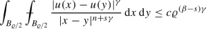  (6.1)

  holds with $c \equiv c (\texttt {data} _{\text {h}}, \texttt {d} ,\beta )$.

• The inequality

  $$\begin{aligned} t^{-\delta }[\texttt {snail} _{\delta }(t)]^{\gamma }\equiv t^{-\delta }[\texttt {snail} _{\delta }(u, B_t(x_0))]^{\gamma } \le c \end{aligned}$$

  (6.2)

  holds whenever $0<t \le \varrho$, where $c \equiv c (\texttt {data} _{\text {h}},\texttt {d} )$.

• If $\lambda >0$, then

  

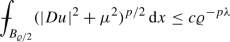  (6.3)

  holds with $c\equiv c(\texttt {data} _{\text {h}}, \texttt {d} ,\lambda )$.

Proof

Estimate in (6.1) follows from Theorem 3 with $\alpha \equiv \beta$. To prove (6.2) we estimate as follows:

$$\begin{aligned} t^{-\delta }[\texttt {snail} _{\delta }(t)]^{\gamma }\le & {} c\int _{{\mathbb {R}}^{n}\setminus B_{\texttt {d}}}\frac{|u(y)-(u)_{B_{t}(x_{0})}|^{\gamma }}{|y-x_{0}|^{n+s\gamma }} \,\textrm{d}y\nonumber \\{} & {} +\,c\int _{B_{\texttt {d} }\setminus B_{t}}\frac{|u(y)-u(x_{0})|^{\gamma }}{|y-x_{0}|^{n+s\gamma }} \,\textrm{d}y\nonumber \\{} & {} +\,c\int _{B_{\texttt {d} }\setminus B_{t}}\frac{|u(x_0)-(u)_{B_{t}(x_{0})}|^{\gamma }}{|y-x_{0}|^{n+s\gamma }} \,\textrm{d}y\nonumber \\\le & {} \frac{c}{\texttt {d} ^{n+s\gamma }}\left( \Vert u\Vert _{L^{\gamma }({\mathbb {R}}^n)}^{\gamma }+\Vert u\Vert _{L^{1}(\Omega _{1})}^{\gamma }\right) \nonumber \\{} & {} +\, c\int _{B_{\texttt {d} }}\frac{\,\textrm{d}y}{|y-x_{0}|^{n+(s-\beta )\gamma } }\, [u]_{0,\beta ;\Omega _1}^{\gamma }\nonumber \\{} & {} +\,ct^{\beta \gamma }\int _{{\mathbb {R}}^n\setminus B_{t}}\frac{\,\textrm{d}y}{|y-x_{0}|^{n+s\gamma }}\, [u]_{0,\beta ;\Omega _1}^{\gamma } \nonumber \\\le & {} c\texttt {d} ^{-n-s\gamma } + c \texttt {d} ^{(\beta -s)\gamma }+ ct^{(\beta -s)\gamma } \le c \,, \end{aligned}$$

(6.4)

where $c\equiv c(\texttt {data} _{\text {h}},\texttt {d} , \beta )$, that is (6.2) if we choose $\beta := (1+s)/2$. Finally, to prove (6.3) we use (4.2) and estimate the various terms stemming from $\texttt {ccp} _{*}(\varrho )\equiv \texttt {ccp} _{*}(u,B_{\varrho }(x_0))$, whose definition is in (3.6). Again by Theorem 3, we have that

$$\begin{aligned} \varrho ^{-p}[\texttt {av} _{p}(\varrho )]^{p}+\varrho ^{-s\gamma }[\texttt {av} _{\gamma }(\varrho )]^{\gamma }\le c\varrho ^{p(\beta -1)}+c\varrho ^{\gamma (\beta -s)}\le c\varrho ^{p(\beta -1)} \end{aligned}$$

holds with $c\equiv c(\texttt {data} _{\text {h}},\texttt {d} ,\beta )$. By (6.2) we instead have

$$\begin{aligned} \varrho ^{-\delta }[\texttt {snail} _{\delta }(\varrho )]^{\gamma }+\Vert f \Vert ^{p/(p-1)}_{L^n(B_{\varrho })}+1\le c\le c\varrho ^{p(\beta -1)}\,. \end{aligned}$$

Choosing $\beta$ such that $1-\beta \le \lambda$, we arrive at (6.3). $\square$

Lemma 6.2

If $h\in u+W^{1,p}_{0}(B_{\varrho /4}(x_{0}))$ is as in (4.6), then

(6.5)

holds where $\sigma _2\equiv \sigma _2(n,p,s,\gamma ,d) \in (0,1)$ and $c\equiv c(\texttt {data} _{\text {h}}, \Vert f\Vert _{L^d(\Omega )},\texttt {d} )$.

Proof

We go back to Lemma 4.2, estimate (4.15), and, adopting the notation introduced there, we improve the estimates for the terms $\text{(I) }$–$\text{(III) }$. As in (4.16) and in Lemma 4.1, we find

(6.6)

for every $\lambda >0$, where $c\equiv c(\texttt {data} _h,\texttt {d} ,\lambda )$. In order to estimate terms (II) and (III), we recall that a basic consequence of the maximum principle is

$$\begin{aligned} \mathop {{{\,\textrm{osc}\,}}}\limits _{B_{\varrho /4}}h\le \mathop {{{\,\textrm{osc}\,}}}\limits _{ B_{\varrho /4}}u\,. \end{aligned}$$

(6.7)

Recall also that u is Hölder continuous; by the Maz’ya-Wiener boundary regularity theory, h is continuous on ${{\bar{B}}}_{\varrho /4}$ and therefore

$$\begin{aligned} \Vert w \Vert _{L^{\infty }(B_{\varrho /4})}= \Vert u-h \Vert _{L^{\infty }(B_{\varrho /4})}{\mathop {\le }\limits ^{(6.7)}} 2\mathop {{{\,\textrm{osc}\,}}}\limits _{\partial B_{\varrho /4}}u \le 4 [u]_{0, \beta ; B_{\varrho /4}}\varrho ^{\beta }\le c\varrho ^{\beta }\,, \end{aligned}$$

(6.8)

where $c\equiv c(\texttt {data} _{\text {h}},\texttt {d} ,\beta )$. For (II), as in (4.17), we have, with $w=u-h$ (defined and extended as in Lemma 4.2, so that $w\equiv 0$ outside $B_{\varrho /4}$)

(6.9)

whenever $s< \beta <1$ and $\lambda >0$, where $c\equiv c(\texttt {data} _n,\texttt {d} ,\beta ,\lambda )$. To estimate $\text{(III) }$ we restart from the fifth line of (4.18), and using also (6.2) and (6.8), we easily find

$$\begin{aligned} |\text{(III) }|\le & {} c\left[ \varrho ^{-s\gamma }[\texttt {av} _{\gamma }(\varrho )]^{\gamma -1}+\varrho ^{-s}\left( \varrho ^{-\delta }[\texttt {snail} _{\delta }(\varrho )]^{\gamma }\right) ^{1-1/\gamma }\right] \Vert w \Vert _{L^{\infty }(B_{\varrho /4})}\nonumber \\\le & {} c\varrho ^{(\beta -s)\gamma }+c\varrho ^{\beta -s}\le c\varrho ^{\beta -s}\,. \end{aligned}$$

(6.10)

In (6.6), (6.9) and (6.10), the numbers $\beta , \lambda$ are arbitrary and such that $s< \beta <1$, $\lambda >0$ and the constants denoted by c depend on $\texttt {data} _{\text {h}},\texttt {d} ,\beta ,\lambda$. We then choose $\beta , \lambda$ such that

$$\begin{aligned} \beta := \frac{1+s}{2}, \qquad 0<\lambda \le \min \left\{ \frac{(1-s)(\gamma -1)}{4}, \frac{1}{2}\left( 1-\frac{n}{d}\right) \right\} \end{aligned}$$

and plug (6.6),(6.9) and (6.10) into (4.15), to obtain

(6.11)

for $c\equiv c(\texttt {data} _{\text {h}}, \Vert f\Vert _{L^d(\Omega )},\texttt {d} )$. Now, we want to finally prove that (6.5) holds with $\sigma _2=\sigma _1$ if $p \ge 2$, and $\sigma _2:=\sigma _1p/4$ if $1<p<2$. Indeed, If $p\ge 2$, then (6.5) follows thanks to (2.9) and (6.11). When $p\in (1,2)$, as in (4.22), and using (4.8), we have

By choosing $\lambda$ such that $\sigma _1p/2-\lambda (1-p/2) > \sigma _1p/4$, we finally conclude with (6.5). $\square$

Once (6.5) is established, we can conclude with the local Hölder continuity of Du by means of a by now classical comparison argument (see for instance [69]). We briefly report it here for the sake of completeness. We recall the following classical decay estimate, which is satisfied by h

(6.12)

that holds whenever $0 < t \le \varrho /8$, where $c \equiv c (n, p, \Lambda )\ge 1$ and $\alpha _0 \equiv \alpha _0(n,p,\Lambda )\in (0,1)$; see [68, 69]. We estimate, also using (3.11)

(6.13)

with $c\equiv c(\texttt {data} _{\text {h}},\texttt {d} ,\lambda )$. In the above inequality, we take $t=\varrho ^{1+\sigma _2p/(2n)}/8$ and choose $\lambda := \sigma _2p\alpha _0/(4n)$ in (6.3). We conclude with

where $c\equiv c(\texttt {data} _{\text {h}},\texttt {d} ,\lambda )$. This holds whenever $B_t\Subset \Omega$ is s ball centred in $\Omega _0$, with $t\le \texttt {d} ^{1+\sigma _2p/(2n)}/c(n,p)$. As the $\Omega _0 \Subset \Omega _1 \Subset \Omega$ are arbitrary, this implies the local $C^{1,\alpha }$-regularity of Du in $\Omega$, via the classical Campanato-Meyers’ integral characterization of Hölder continuity together with the estimate for $[Du]_{0,\alpha ; \Omega _0}$, and the proof is complete.

Remark 5

The content of Remark 3 applies to the above proof as well.

7 Distributional solutions

• In this paper we mainly deal with minimizers. For these the Euler–Lagrange equation (1.11) holds automatically for every $\varphi \in {\mathbb {X}}_{0}(\Omega )$ in the setting of Theorems 3–5 (by the way, notice that no Lipschitz continuity of $\Omega$ is needed for this). This motivates the definition of weak solution in (1.15) with $\varphi \in {\mathbb {X}}_{0}(\Omega )$. One might of course wonder what happens when taking as tests in (1.15) functions $\varphi \in C^{\infty }_{0}(\Omega )$, thereby considering classical distributional solutions. This actually gives rise to the same notion of solution. Indeed, thanks to the Lipschitz regularity of $\partial \Omega$, we can use the argument in [12, Proposition B.1] to deduce that, given $\varphi \in {\mathbb {X}}_{0}(\Omega )$, there exists a sequence $\{\varphi _k\}\subset C^{\infty }_{0}(\Omega )$ such that $\varphi _k\rightarrow \varphi$ in $W^{1,p}(\Omega )$ and $W^{s,\gamma }({\mathbb {R}}^n)$. A standard application of Lebesgue dominated convergence then implies that a distributional solution to (1.15) also satisfies (1.15) for every $\varphi \in {\mathbb {X}}_{0}(\Omega )$.

• The above point is useful if one wants to connect equations of the type in (1.15) with minimizers as considered in Theorems 3–5. Of course, when proving interior regularity, one can also define more local solutions to (1.15) by requiring that (1.15) is satisfied for every $\varphi \in C^{\infty }_{0}(\Omega )$. In this case one can starts by solutions $u\in W^{1,p}_{{\text {loc}}}(\Omega )\cap W^{s,\gamma }({\mathbb {R}}^n)$; no Lipschitz regularity of $\Omega$ is needed in this case. Moreover, one can assume $f \in L^n_{{\text {loc}}}(\Omega )$ and $f \in L^d_{{\text {loc}}}(\Omega )$ in Theorems 3 and 5, respectively.

8 Further directions, open problems

The results of this paper pose several questions and problems. Without pretending to be exhaustive concerning the directions one might take, we give a short list of possible issues here.

8.1 Optimal assumptions on the data and borderline regularity

In Theorem 7 it should be possible to replace the assumption $f\in L^q(\Omega )$ by $f \in {\mathcal {M}}^q(\Omega )$, the Marcinkiwicz space, this meaning that

$$\begin{aligned} \sup _{\lambda>0} \, \lambda ^{q}\, |\{|f|>\lambda \}| < \infty . \end{aligned}$$

As for the borderline regularity in terms of solutions, it is reasonable to conjecture that, under the assumptions of Theorems 4

$$\begin{aligned} {\left\{ \begin{array}{ll} 1<p< n \text{ and } f \in L\left( \frac{n}{p}, \frac{1}{p-1} \right) \Longrightarrow u \text{ is } \text{ continuous }\,.\\ p=n \text{ and } f \in L^1 \Longrightarrow u\in BMO, \text{ locally }\,. \end{array}\right. } \end{aligned}$$

In the first line above there appears the borderline Lorentz space, while in the second we see John–Nirenberg space of functions with bounded mean oscillations. These conjectured facts, are, as Theorem 7, in line with the theory of local operators. We refer to [58, Section 9] for an overview to use as a guide to build parallels with the local theory, and for the definitions of the above spaces. As for the gradient, under the assumptions of Theorem 5 the conjectured borderline regularity claims that if $f \in L(n,1)$, then Du is continuous. This is true in the local case [57], and we expect it to hold in the mixed one too.

8.2 Boundary regularity

The assumptions (1.8)$_{2,3}$ prescribe that the Hölder continuity of g is a consequence of its higher gradient integrability (both in classical and fractional sense) via Sobolev–Morrey embedding. As mentioned in Remark 1, this is a common approach in the literature. It is nevertheless tempting to replace (1.8)$_{2,3}$ via a direct Hölder continuity assumption as $g\in W^{1,p}(\Omega )\cap W^{s,\gamma }({\mathbb {R}}^{n})\cap C^{0, \kappa }(\Omega )$. This brings the problem to the completely different realm of a quantitative Wiener criterion, that already in the local case needs completely different approaches and tools. Some of these, are not yet fully available in the nonlocal case. See for instance the approaches in [65]; se also [53, 72] for references. We leave these questions as an interesting open issue and we anyway note that the usually treated boundary regularity problems in the nonlocal literature deals with the case $g\equiv 0$ [51, 52, 75].

8.3 The case $\gamma >p$ and boundedness of solutions

By looking at Theorems 3, 5 and especially 6, a question naturally arises concerning the possibility of removing, when $\gamma >p$, the (local) boundedness assumption on u, or, equivalently via Proposition 2.1, assumption (1.9). The case $\gamma >p$ is actually the one where the problem in question resembles, and actually shares a few features with, those with nonuniform ellipticity (non-standard growth conditions [70, 71]). In fact, the approach via bounded solutions or boundary data taken here draws a parallel with the situation observed in nonuniformly elliptic problems; see for instance [32] for an overview and the basic definitions. In order to fix the ideas, we consider the double phase integral, that is

$$\begin{aligned} w \mapsto \int _{\Omega } (|Dw|^p+a(x)|Dw|^{q})\, dx\,, \quad C^{0, \alpha }(\Omega ) \ni a(\cdot )\ge 0\,, \quad 1<p \le q\,. \end{aligned}$$

(8.1)

In this case minima are Hölder regular provided the sharp dimensional condition

$$\begin{aligned} \frac{q}{p} \le 1 +\frac{\alpha }{n} \end{aligned}$$

(8.2)

is met. Instead, when minimizers are known to be bounded, condition (8.2) improves in the non-dimensional one

$$\begin{aligned} q \le p +\alpha \,, \end{aligned}$$

(8.3)

which is also sharp (see [26, 30] and related references, and [40] for the sharpness of (8.2) and (8.3)). The improvement goes via interpolation estimates of the type for instance considered in Lemma 2.3 from this paper. The integrand of the functional in (8.1) is built upon two different elliptic terms, whose interaction is anyway problematic as conditions (8.2)-(8.3) are indeed necessary to guarantee regularity. In the present setting the role of the highest exponent q in (8.1) should be played by $\gamma >p$, so that the condition $p>s\gamma$ plays the role of (8.3). Note that such a bound alone does not imply the imbedding $W^{1,p}\subset W^{s,\gamma }$ (this is in fact fixed via interpolation for bounded functions as in Lemma 2.3). Moreover, note that both (8.3) and $p>s\gamma$ are basically capacitary conditions.

Back to the parallel with local nonuniformly elliptic problems, let us note that the boundedness assumption on minima is usually satisfied using the maximum principle in presence of bounded boundary data. This is again in line with what we do in Proposition 2.1. This discussion then leads to think that, in the spirit of (8.2), a condition as

$$\begin{aligned} \frac{\gamma }{p} < 1 + \texttt {o}(n), \qquad \lim _{n\rightarrow \infty } \, \texttt {o}(n)=0 \end{aligned}$$

could be sufficient to establish the local boundedness of solutions and then to conclude with Theorems 3-(6) without assuming (1.9). Such conditions are typical and actually necessary in the setting of nonuniformly elliptic problems with nonstandard growth conditions [71].

References

Adams, R.A., Fournier, J.F.: Sobolev Spaces. Pure and Applied Mathematics (Amsterdam), vol. 140, 2nd edn., p. xiv+305. Elsevier/Academic Press, Amsterdam (2003)
Avelin, B., Kuusi, T., Mingione, G.: Nonlinear Calderön–Zygmund theory in the limiting case. Arch. Ration. Mech. Anal. 227, 663–714 (2018)
Barles, G., Imbert, C.: Second-order elliptic integro-differential equations: viscosity solutions’ theory revisited. Ann. Inst. H. Poincé C Anal. Non Linéaire 25, 567–585 (2008)
Beck, L.: Boundary regularity results for weak solutions of subquadratic elliptic systems. Ph.D. Thesis, Erlangen (2008)
Beck, L.: Boundary regularity for elliptic problems with continuous coefficients. J. Convex Anal. 16, 287–320 (2009)
Biagi, S., Dipierro, S., Valdinoci, E., Vecchi, E.: Mixed local and nonlocal elliptic operators: regularity and maximum principles. Commun. PDE 47, 585–629 (2022)
Biagi, S., Dipierro, S., Valdinoci, E., Vecchi, E.: Semilinear elliptic equations involving mixed local and nonlocal operators. Proc. R. Soc. Edinb. A Math. 151, 1611–1641 (2021)
Biagi, S., Dipierro, S., Valdinoci, E., Vecchi, E.: A Faber–Krahn inequality for mixed local and nonlocal operators. arXiv:2104.00830
Biagi, S., Dipierro, S., Valdinoci, E., Vecchi, E.: A Hong–Krahn–Szegö inequality for mixed local and nonlocal operators. Math. Eng. 5(1), 1–25 (2022)
Brasco, L., Lindgren, E.: Higher Sobolev regularity for the fractional \(p\)-Laplace equation in the superquadratic case. Adv. Math. 304, 300–354 (2017)
Brasco, L., Lindgren, E., Schikorra, A.: Higher Hölder regularity for the fractional \(p\)-Laplacian in the superquadratic case. Adv. Math. 338, 782–846 (2018)
Brasco, L., Parini, E.: The second eigenvalue of the fractional \(p\)-Laplacian. Adv. Calc. Var. 9, 323–355 (2016)
Brasco, L., Parini, E., Squassina, M.: Stability of variational eigenvalues for the fractional \(p\)-Laplacian. Discrete Contin. Dyn. Syst. 36, 1813–1845 (2016)
Brezis, H., Mironescu, P.: Gagliardo–Nirenberg, composition and products in fractional Sobolev spaces. J. Evol. Equ. 1, 387–404 (2001)
Brezis, H., Mironescu, P.: Gagliardo–Nirenberg inequalities and non-inequalities: the full story. Ann. IHP-AN 35, 1355–1376 (2018)
Byun, S.S., Kim, H., Ok, J.: Local Hölder continuity for fractional nonlocal equations with general growth. Math. Ann. (To appear)
Byun, S.S., Ok, J., Song, K.: Hölder regularity for weak solutions to nonlocal double phase problems. arXiv:2108.09623
Chaker, J., Kassmann, M.: Nonlocal operators with singular anisotropic kernels. Commun. PDE 45(1), 1–31 (2020)
Chaker, J., Kim, M.: Regularity estimates for fractional orthotropic \(p\)-Laplacians of mixed order. Adv. Nonlinear Anal. 11, 1307–1331 (2022)
Chaker, J., Kim, M., Weidner, M.: Regularity for nonlocal problems with non-standard growth. arXiv:2111.09182 (2022)
Chan, Y., DiBenedetto, E.: Boundary estimates for solutions of nonlinear degenerate parabolic systems. J. Reine Angew. Math. 395, 102–131 (1989)
Chen, Z.-Q., Kim, P., Song, R., Vondraček, Z.: Sharp Green function estimates for \(\Delta +\Delta ^{\alpha /2}\) in \(C^{1,1}\) open sets and their applications. Ill. J. Math. 54, 981–1024 (2010)
Chen, Z.-Q., Kim, P., Song, R., Vondraček, Z.: Boundary Harnack principle for \(\Delta +\Delta ^{\alpha /2}\). Trans. Am. Math. Soc. 364, 4169–4205 (2012)
Chen, Z.-Q., Kumagai, T.: A priori Hölder estimate, parabolic Harnack principle and heat kernel estimates for diffusions with jumps. Rev. Mat. Iberoam. 26, 551–589 (2010)
Cianchi, A.: Maximizing the \(L^{\infty }\) norm of the gradient of solutions to the Poisson equation. J. Geom. Anal. 2, 499–515 (1992)
Colombo, M., Mingione, G.: Calderón–Zygmund estimates and non-uniformly elliptic operators. J. Funct. Anal. 270, 1416–1478 (2016)
Da Silva, J.V., Salort, A.M.: A limiting problem for local/non-local \(p\)-Laplacians with concave-convex nonlinearities. Z. Angew. Math. Phys. 71(6), 191 (2020)
De Filippis, C.: Quasiconvexity and partial regularity via nonlinear potentials. J. Math. Pures Appl. 9(163), 11–82 (2022)
De Filippis, C., Mingione, G.: On the regularity of minima of non-autonomous functionals. J. Geom. Anal. 30, 1584–1626 (2020)
De Filippis, C., Mingione, G.: Manifold constrained non-uniformly elliptic problems. J. Geom. Anal. 30, 1661–1723 (2020)
De Filippis, C., Mingione, G.: Interpolative gap bounds for nonautonomous integrals. Anal. Math. Phys. 11, 117 (2021)
De Filippis, C., Mingione, G.: Lipschitz bounds and nonautonomous integrals. Arch. Ration. Mech. Anal. 242, 973–1057 (2021)
De Filippis, C., Palatucci, G.: Hölder regularity for nonlocal double phase equations. J. Differ. Equ. 267, 547–586 (2019)
DeVore, R., Sharpley, R.C.: Maximal functions measuring smoothness. Mem. Am. Math. Soc. 47(293) (1984)
Di Castro, A., Kuusi, T., Palatucci, G.: Local behavior of fractional \(p\)-minimizers. Ann. IHP-AN 33, 1279–1299 (2016)
Di Castro, A., Kuusi, T., Palatucci, G.: Nonlocal Harnack inequalities. J. Funct. Anal. 267, 1807–1836 (2014)
Di Nezza, E., Palatucci, G., Valdinoci, E.: Hitchhiker’s guide to the fractional Sobolev spaces. Bull. Sci. Math. 136(5), 521–573 (2012)
Dipierro, S., Lippi, E.P., Valdinoci, E.: (Non)local logistic equations with Neumann conditions. arXiv:2101.02315
Duzaar, F., Grotowski, J., Kronz, M.: Partial and full boundary regularity for minimizers of functionals with nonquadratic growth. J. Convex Anal. 11, 437–476 (2004)
Esposito, L., Leonetti, F., Mingione, G.: Sharp regularity for functionals with \((p, q)\) growth. J. Differ. Equ. 204, 5–55 (2004)
Fang, Y., Shang, B., Zhang, C.: Regularity theory for mixed local and nonlocal parabolic \(p\)-Laplace equations. J. Geom. Anal. 32, 22 (2022)
Fang, Y., Zhang, C.: On Weak and viscosity solutions of nonlocal double phase equations. Int. Math. Res. Not. (2021). https://doi.org/10.1093/imrn/rnab351
Fernández Bonder, J., Salort, A., Vivas, H.: Interior and up to the boundary regularity for the fractional \(g\)-Laplacian: the convex case. Nonlinear Anal. 223, 113060 (2022)
Foondun, M.: Heat kernel estimates and Harnack inequalities for some Dirichlet forms with non-local part. Electron. J. Probab. 14, 314–340 (2009)
Garain, P., Kinnunen, J.: On the regularity theory for mixed local and nonlocal quasilinear elliptic equations. Trans. Am. Math. Soc. 375, 5393–5423 (2022)
Garain, P., Lindgren, E.: Higher Hölder regularity for mixed local and nonlocal degenerate elliptic equations. arXiv:2204.13196v1
Giaquinta, M., Giusti, E.: Differentiability of minima of non-differentiable functionals. Invent. Math. 72, 285–298 (1983)
Giusti, E.: Direct Methods in the Calculus of Variations. World Scientific Publishing Co., Inc, River Edge (2003)
Hamburger, C.: Regularity of differential forms minimizing degenerate elliptic functionals. J. Reine Angew. Math. (Crelles J.) 431, 7–64 (1992)
Hirsch, M.W.: Differential Topology, GMT, No. 33. Springer, New York (1976)
Iannizzotto, A., Mosconi, S., Squassina, M.: Global Hölder regularity for the fractional \(p\)-Laplacian. Rev. Mat. Iberoam. 32, 1353–1392 (2016)
Iannizzotto, A., Mosconi, S., Squassina, M.: Fine boundary regularity for the degenerate fractional \(p\)-Laplacian. J. Funct. Anal. 279, 108659 (2020)
Kim, M., Lee, K.A., Lee, S.C.: The Wiener criterion for nonlocal Dirichlet problems. arXiv:2203.16815
Koch, L.: Global higher integrability for minimisers of convex obstacle problems with \((p, q)\)-growth. Calc. Var. PDE 61, 88 (2022)
Korvenpää, J., Kuusi, T., Lindgren, E.: Equivalence of solutions to fractional \(p\)-Laplace type equations. J. Math. Pures Appl. 9(132), 1–26 (2019)
Korvenpää, J., Kuusi, T., Palatucci, G.: The obstacle problem for nonlinear integro-differential operators. Calc. Var. PDE 55, 63 (2016)
Kuusi, T., Mingione, G.: A nonlinear Stein theorem. Calc. Var. PDE 51, 45–86 (2014)
Kuusi, T., Mingione, G.: Guide to nonlinear potential estimates. Bull. Math. Sci. 4, 1–82 (2014)
Kuusi, T., Mingione, G., Sire, Y.: Nonlocal equations with measure data. Commun. Math. Phys. 337, 1317–1368 (2015)
Kuusi, T., Mingione, G., Sire, Y.: Nonlocal self-improving properties. Anal. PDE 8, 57–114 (2015)
Kristensen, J., Melcher, C.: Regularity in oscillatory nonlinear elliptic systems. Math. Z. 260, 813–847 (2008)
Kronz, M.: Boundary regularity for almost minimizers of quasiconvex variational problems. NoDEA 12, 351–382 (2005)
Ladyzhenskaya, O.A., Ural’tseva, N.N.: Linear and Quasilinear Elliptic Equations. Academic Press Inc., Amsterdam (1968)
Lewis, J.L.: Smoothness of certain degenerate elliptic equations. Proc. Am. Math. Soc. 80, 259–265 (1980)
Lian, Y., Zhang, K., Li, D., Hong, G.: Boundary Hölder regularity for elliptic equations. J. Math. Pures Appl. 143(9), 311–333 (2020)
Lieberman, G.M.: The natural generalization of the natural conditions of Ladyzhenskaya and Ural’tseva for elliptic equations. Commun. PDE 16, 311–361 (1991)
Lindgren, E.: Hölder estimates for viscosity solutions of equations of fractional \(p\)-Laplace type. NoDEA 23(5), 55 (2016)
Manfredi, J.J.: Regularity of the gradient for a class of nonlinear possibly degenerate elliptic equations. Ph.D. Thesis, University of Washington, St. Louis (1986)
Manfredi, J.J.: Regularity for minima of functionals with \(p\)-growth. J. Differ. Equ. 76, 203–212 (1988)
Marcellini, P.: Regularity of minimizers of integrals of the calculus of variations with non standard growth conditions. Arch. Ration. Mech. Anal. 105, 267–284 (1989)
Marcellini, P.: Regularity and existence of solutions of elliptic equations with \(p, q\)-growth conditions. J. Differ. Equ. 90, 1–30 (1991)
Palatucci, G.: The Dirichlet problem for the \(p\)-fractional Laplace equation. Nonlinear Anal. 177, 699–732 (2018)
Scott, J.M., Mengesha, T.: Self-improving inequalities for bounded weak solutions to nonlocal double phase equations. Commun. Pure Appl. Anal. 21, 183–212 (2022)
Soave, N., Tavares, H., Terracini, S., Zilio, A.: Variational problems with long-range interaction. Arch. Ration. Mech. Anal. 228, 743–772 (2018)
Ros-Oton, X., Xavier, J.: Serra: the Dirichlet problem for the fractional Laplacian: regularity up to the boundary. J. Math. Pures Appl. 101(9), 275–302 (2014)
Triebel, H.: Theory of Function Spaces. Birkhäuser, Basel and Boston (1983)
Uhlenbeck, K.: Regularity for a class of non-linear elliptic systems. Acta Math. 138, 219–240 (1977)
Ural’tseva, N.N.: Degenerate quasilinear elliptic systems. Zap. Na. Sem. Leningrad. Otdel. Mat. Inst. Steklov. (LOMI) 7, 184–222 (1968)
Acknowledgements
The present version of the paper has benefited a lot from the inputs received by an anonymous referee, who examined a first draft with extraordinary care and delivered very valuable comments and viewpoints. This work is supported by the University of Parma via the project “Regularity, Nonlinear Potential Theory and related topics”. The first author is supported by the INdAM GNAMPA project “Fenomeni non locali in problemi locali”.
Funding
Open access funding provided by Università degli Studi di Parma within the CRUI-CARE Agreement.
Author information
Authors and Affiliations
Corresponding author
Ethics declarations
Conflict of interest
The authors declare to have no conflict of interests. No data are attached to this paper.
Additional information
Publisher's Note
Springer Nature remains neutral with regard to jurisdictional claims in published maps and institutional affiliations.
Rights and permissions
Open Access This article is licensed under a Creative Commons Attribution 4.0 International License, which permits use, sharing, adaptation, distribution and reproduction in any medium or format, as long as you give appropriate credit to the original author(s) and the source, provide a link to the Creative Commons licence, and indicate if changes were made. The images or other third party material in this article are included in the article’s Creative Commons licence, unless indicated otherwise in a credit line to the material. If material is not included in the article’s Creative Commons licence and your intended use is not permitted by statutory regulation or exceeds the permitted use, you will need to obtain permission directly from the copyright holder. To view a copy of this licence, visit http://creativecommons.org/licenses/by/4.0/.
About this article
Cite this article
De Filippis, C., Mingione, G. Gradient regularity in mixed local and nonlocal problems. Math. Ann. 388, 261–328 (2024). https://doi.org/10.1007/s00208-022-02512-7
Received:
Revised:
Accepted:
Published:
Issue Date:
DOI: https://doi.org/10.1007/s00208-022-02512-7