
Abstract
We discuss a parabolic version of the space of functions of bounded mean oscillation related to a doubly nonlinear parabolic partial differential equation. Parabolic John–Nirenberg inequalities, which give exponential decay estimates for the oscillation of a function, are shown in the natural geometry of the partial differential equation. Chaining arguments are applied to change the time lag in the parabolic John–Nirenberg inequality. We also show that the quasihyperbolic boundary condition is a necessary and sufficient condition for a global parabolic John–Nirenberg inequality. Moreover, we consider John–Nirenberg inequalities with medians instead of integral averages and show that this approach gives the same class of functions as the original definition.
1 Introduction
Functions of bounded mean oscillation (\(\mathrm {BMO}\)) are essential in harmonic analysis and partial differential equations. A particularly useful result is the John–Nirenberg lemma which gives an exponential decay estimate for the mean oscillation of a function in \(\mathrm {BMO}\). Functions of bounded mean oscillation and the John–Nirenberg lemma were first discussed in [11] and the corresponding time-dependent theory was initiated by Moser in [18, 19]. The proof of the parabolic John–Nirenberg lemma requires genuinely new ideas compared to the time independent case. The main challenge is that the definition of parabolic \(\mathrm {BMO}\) consists of two conditions on the mean oscillation of a function, one in the past and the other one in the future with a time lag between the estimates, see Definition 2.4 below. Moreover, Euclidean cubes are replaced by rectangles that respect the natural geometry of the related parabolic partial differential equation. Fabes and Garofalo [6] gave a simpler proof for the parabolic John–Nirenberg lemma and the general approach of Aimar [1] applies in spaces of homogeneous type. Martín-Reyes and de la Torre [17] studied one-sided \(\mathrm {BMO}\) in the one-dimensional case. Berkovits [2, 3] discussed this approach in the higher dimensional case, but the geometry is not related to nonlinear parabolic partial differential equations. In contrast with the extensive literature on the classical \(\mathrm {BMO}\), there are few references to the corresponding parabolic theory.
We discuss a parabolic \(\mathrm {BMO}\) space tailored to a doubly nonlinear equation
For \(p=2\) we have the standard heat equation. Gradient and divergence are taken with respect to the spatial variable only. Observe that a solution to (1.1) can be scaled, but constants cannot be added to a solution. The equation is nonlinear in the sense that the sum of two solutions is not a solution in general. Our discussion applies to more general equations of the type
where A is a Caratheodory function that satisfies the structural conditions
for some positive constants \(C_0\) and \(C_1\). In the natural geometry of (1.1), we consider space-time rectangles where the time variable scales to the power p. This is in accordance with the following scaling property: if u(x, t) is a solution, so does \(u(\alpha x,\alpha ^p t)\) with \(\alpha >0\). Different values of p lead to different p-geometries and different parabolic \(\mathrm {BMO}\) spaces. For recent regularity results for the doubly nonlinear equation, we refer to Bögelein, Duzaar, Kinnunen and Scheven [5], Bögelein, Duzaar and Liao [4], Kuusi, Siljander and Urbano [15] and Kuusi, Laleoglu, Siljander and Urbano [16].
The following scale and location invariant Harnack inequality for positive solutions to (1.1) has been obtained by Moser [18] for \(p=2\) and by Trudinger [26] for \(1<p<\infty \). See also Gianazza and Vespri [8] and Kinnunen and Kuusi [12]. Assume that \(u>0\) is a weak solution to (1.1) in \(\Omega _T=\Omega \times (0,T)\) and let \(0<\gamma <1\) be a time lag. There exist an exponent \(\delta =\delta (n,p,\gamma )>0\) and constants \(c_i=c_i(n,p,\gamma )>0\), \(i=1,2,3\), such that

for every parabolic rectangle with \(2R\subset \Omega _T\). See Definition 2.1 for the parabolic rectangles. Harnack’s inequality gives a scale and location invariant pointwise bound for a positive solution at a given time in terms of its values at later times. This indicates that the parabolic rectangles in the p-geometry respect the natural geometry of the doubly nonlinear equation. The time lag \(\gamma >0\) is an unavoidable feature of the theory rather than a mere technicality. The fact that the result is not true with \(\gamma =0\) can be seen from the heat kernel already when \(p=2\), since Harnack’s inequality does not hold on a given time slice. The first and the last inequalities in (1.2) are based on a successive application of Sobolev’s inequality and energy estimates. The remaining inequality follows from the fact that a logarithm of a positive weak solution belongs to the parabolic \(\mathrm {BMO}\) with a uniform estimate and a parabolic John–Nirenberg lemma as in [18, 26]. The proof in [12] applies an abstract lemma of Bombieri instead of the parabolic John–Nirenberg lemma. See also Kinnunen and Saari [13] and Saari [22]. The parabolic John–Nirenberg lemma with a general parameter p has applications in the theory of parabolic Muckenhoupt weights in Kinnunen and Saari [13, 14].
We discuss several versions of the parabolic John–Nirenberg inequality in the p-geometry with \(1<p<\infty \). Theorem 3.1 gives an exponential bound for the mean oscillation in terms of integral averages. To our knowledge this result is new already for \(p=2\) and generalizes the corresponding result for the standard \(\mathrm {BMO}\) in [11] to the parabolic case. A more common version of the parabolic John–Nirenberg inequality is stated in Corollary 3.2. This generalizes the results of Moser [18, 19] and Fabes and Garofalo [6] to the p-geometry with \(1<p<\infty \). A general approach of Aimar [1] applies in metric measure spaces and also covers the p-geometry with \(1<p<\infty \) by considering the parabolic metric
We prefer giving a direct and transparent proof in the p-geometry that also allows further investigation of the theory of parabolic \(\mathrm {BMO}\). The argument is based on a Calderón–Zygmund decomposition in the p-geometry. The John–Nirenberg inequality implies that a parabolic \(\mathrm {BMO}\) function is locally integrable to any positive power with reverse Hölder-type bounds, see Corollary 3.3. Corollary 5.4 gives a stronger result which states that a parabolic \(\mathrm {BMO}\) function is locally exponentially integrable with uniform estimates on parabolic rectangles. A chaining argument in the proof of Theorem 4.1 shows that the size of the time lag can be changed in parabolic \(\mathrm {BMO}\). Parabolic chaining arguments have been previously studied by Saari [22, 23] and our approach complements these techniques. We also discuss the John–Nirenberg inequality up to the spatial boundary of a space-time cylinder by applying results of Saari [22] and Smith and Stegenga [24]. In particular, we show that the quasihyperbolic boundary condition is a necessary and sufficient condition for a global parabolic John–Nirenberg inequality. This extends some of the results in [24] to the parabolic setting.
John [10] observed that it is possible to relax the a priori local integrability assumption in the definition of \(\mathrm {BMO}\) and to create a theory that applies to measurable functions. We extend this theory to the parabolic context. This approach is based on the notion of median, for example, see Jawerth and Torchinsky [9], Poelhuis and Torchinsky [21] and Strömberg [25]. It is remarkable that the John–Nirenberg inequality can be proved starting from this condition and as a consequence, these functions are locally integrable to any positive power, see Theorem 6.6. Corollary 6.8 shows that the parabolic \(\mathrm {BMO}\) with medians coincides with the original definition of parabolic \(\mathrm {BMO}\).
2 Definition and properties of parabolic \(\mathrm {BMO}\)
The underlying space throughout is \({\mathbb {R}}^{n+1}=\{(x,t):x=(x_1,\dots ,x_n)\in \mathbb R^n,t\in \mathbb R\}\). Unless otherwise stated, constants are positive and the dependencies on parameters are indicated in the brackets. The Lebesgue measure of a measurable subset A of \({\mathbb {R}}^{n+1}\) is denoted by \(|A|\). A cube Q is a bounded interval in \(\mathbb R^n\), with sides parallel to the coordinate axes and equally long, that is, \(Q=Q(x,L)=\{y \in \mathbb R^n: |y_i-x_i|\le L,\,i=1,\dots ,n\}\) with \(x\in \mathbb R^n\) and \(L>0\). The point x is the center of the cube and L is the side length of the cube. Instead of Euclidean cubes, we work with the following collection of parabolic rectangles in \({\mathbb {R}}^{n+1}\).
Definition 2.1
Let \(1<p<\infty \), \(x\in \mathbb R^n\), \(L>0\) and \(t \in {\mathbb {R}}\). A parabolic rectangle centered at (x, t) with side length L is
and its upper and lower parts are
where \(-1< \gamma < 1\) is called the time lag.
Note that \(R^-(\gamma )\) is the reflection of \(R^+(\gamma )\) with respect to the time slice \({\mathbb {R}}^n \times \{t\}\). The spatial side length of a parabolic rectangle R is denoted by \(l_x(R)=L\) and the time length by \(l_t(R)=2L^p\). For short, we write \(R^\pm \) for \(R^{\pm }(0)\). The top of a rectangle \(R = R(x,t,L)\) is \(Q(x,L) \times \{t+L^p\}\) and the bottom is \(Q(x,L) \times \{t-L^p\}\). The \(\lambda \)-dilate of R with \(\lambda >0\) is denoted by \(\lambda R = R(x,t,\lambda L)\). We observe that the Lebesgue differentiation theorem holds on the collection of parabolic rectangles.
Definition 2.2
A sequence \((A_i)_{i\in \mathbb N}\) of measurable sets \(A_i\subset \mathbb R^{n+1}\), \(i\in {\mathbb {N}}\), converges regularly to a point \((x,t) \in {\mathbb {R}}^{n+1}\), if there exist a constant \(c>0\) and a sequence \((R_i)_{i\in \mathbb N}\) of parabolic rectangles \(R_i\), \(i\in {\mathbb {N}}\), such that \(|R_i |\rightarrow 0\) as \(i\rightarrow \infty \), \(A_i \subset R_i\), \((x,t) \in R_i\) and \(|A_i |\le |R_i |\le c |A_i |\) for every \(i \in {\mathbb {N}}\).
The integral average of \(f \in L^1(A)\) in measurable set \(A\subset {\mathbb {R}}^{n+1}\), with \(0<|A|<\infty \), is denoted by

The Lebesgue differentiation theorem below can be proven in a similar way as in the classical case using a covering argument for parabolic rectangles.
Lemma 2.3
Let \(f \in L^1_{\mathrm {loc}}({\mathbb {R}}^{n+1})\). Then

for almost every \((x,t) \in {\mathbb {R}}^{n+1}\), whenever \((A_i)_{i\in \mathbb N}\) is a sequence of measurable sets converging regularly to (x, t).
The positive and the negative parts of a function f are denoted by
Let \(\Omega \subset {\mathbb {R}}^{n}\) be an open set and \(T>0\). A space-time cylinder is denoted by \(\Omega _T=\Omega \times (0,T)\). It is possible to consider space-time cylinders \(\Omega \times (t_1,t_2)\) with \(t_1<t_2\), but we focus on \(\Omega _T\).
This section discusses basic properties of parabolic \(\mathrm {BMO}\). We begin with the definition. The differentials \(\, d x\, d t\) in integrals are omitted in the sequel.
Definition 2.4
Let \(\Omega \subset {\mathbb {R}}^{n}\) be a domain, \(T>0\), \( -1< \gamma < 1\), \( -\gamma \le \delta < 1\) and \(0< q < \infty \). A function \(f \in L_{\mathrm {loc}}^q(\Omega _T)\) belongs to \(\mathrm {PBMO}_{\gamma ,\delta ,q}^{+}(\Omega _T)\) if

If the condition above holds with the time axis reversed, then \(f \in \mathrm {PBMO}_{\gamma ,\delta ,q}^{-}(\Omega _T)\).
For \(0 \le \delta = \gamma < 1\), we abbreviate \(\mathrm {PBMO}_{\gamma ,q}^{+}(\Omega _T) = \mathrm {PBMO}_{\gamma ,\delta ,q}^{+}(\Omega _T)\). In addition, we shall write \(\mathrm {PBMO}^{+}\) and \(\left\Vert {f}\right\Vert \) whenever parameters are clear from the context or are not of importance. Observe that \(f \in L_{\mathrm {loc}}^q(\Omega _T)\) belongs to PBMO\(_{\gamma ,\delta ,q}^{+}(\Omega _T)\) if and only if for every parabolic rectangle R there exists a constant \(c\in \mathbb R\), that may depend on R, with

where \(M\in \mathbb R\) is a constant that is independent of R.
Remark 2.5
Assume that \(u>0\) is a weak solution to the doubly nonlinear equation in \(\Omega _T\) and let \(0<\gamma <1\). By Kinnunen and Saari [13] and Saari [22], we have
with \(q=(p-1)/2\) and
Observe that \(0<q<1\) for \(p<3\). By Hölder’s inequality, we may take \(q=1\) for \(p\ge 3\). Observe that the bound for the \(\mathrm {PBMO}\) norm is independent of the solution.
Example 2.6
Let \(1<p<\infty \) and \(0<\gamma <1\). The function
is a solution of the doubly nonlinear equation in the upper half space \(\mathbb R^n\times (0,\infty )\). By Remark 2.5, we conclude that the function
belongs to \(\mathrm {PBMO}_{\gamma ,q}^{+}(\mathbb R^n\times (0,\infty ))\) with \(q=(p-1)/2\). Corollary 4.2 below implies that f belongs to \(\mathrm {PBMO}_{\gamma ,q}^{+}(\mathbb R^n\times (0,\infty ))\) for every \(0<q<\infty \).
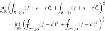
The next lemma shows that for every parabolic rectangle R, there exists a constant \(c_R\), depending on R, for which the infimum in the definition above is attained. In the sequel, this minimal constant is denoted by \(c_R\).
Lemma 2.7
Let \(\Omega _T \subset {\mathbb {R}}^{n+1}\) be a space-time cylinder, \( -1< \gamma < 1\), \( -\gamma \le \delta < 1\) and \(0< q < \infty \). Assume that \(f\in \mathrm {PBMO}_{\gamma ,\delta ,q}^{+}(\Omega _T)\). Then for every parabolic rectangle \(R\subset \Omega _T\), there exists a constant \(c_R\in \mathbb R\), that may depend on R, such that

In particular, it holds that

Proof
Let \(R \subset \Omega _T\) be a parabolic rectangle. Consider a sequence \((c_i)_{i\in \mathbb N}\) of real numbers such that

for every \(i \in {\mathbb {N}}\). Note that

for every \(i \in {\mathbb {N}}\), since \(f \in L_{\mathrm {loc}}^q(\Omega _T)\). If \(0< q \le 1\), then it holds that

This implies

for every \(i \in {\mathbb {N}}\). On the other hand, if \(1< q < \infty \), we have

and thus

for every \(i \in {\mathbb {N}}\). This shows that the sequence \((c_i)_{i\in \mathbb N}\) is bounded. Therefore, there exists a subsequence \((c_{i_k})_{k\in \mathbb N} \) that converges to \(c_R \in {\mathbb {R}}\). Then \((f-c_{i_k})_\pm \) converges uniformly to \((f-c_R)_\pm \) in R as \(k \rightarrow \infty \). This implies the convergence in \(L^q(R)\), and thus

This completes the proof. \(\square \)
We list some properties of parabolic \(\mathrm {BMO}\) below. In particular, parabolic \(\mathrm {BMO}\) is closed under addition and scaling by a positive constant. On the other hand, multiplication by negative constants reverses the time direction.
Lemma 2.8
Let \( -1< \gamma < 1\), \( -\gamma \le \delta < 1\) and \(0< q < \infty \). Assume that f and g belong to \(\mathrm {PBMO}_{\gamma ,\delta ,q}^{+}(\Omega _T)\) and let \(\mathrm {PBMO}^{\pm }=\mathrm {PBMO}_{\gamma ,\delta ,q}^{\pm }(\Omega _T)\). Then the following properties hold true.
-
(i)
\(\left\Vert {f+a}\right\Vert _{\mathrm {PBMO}^{+}} = \left\Vert {f}\right\Vert _{\mathrm {PBMO}^{+}},\, a \in {\mathbb {R}}\).
-
(ii)
\(\left\Vert {f+g}\right\Vert _{\mathrm {PBMO}^{+}} \le \max \{ 2^{\frac{1}{q}-1} , 2^{1-\frac{1}{q}} \} \left( \left\Vert {f}\right\Vert _{\mathrm {PBMO}^{+}} + \left\Vert {g}\right\Vert _{\mathrm {PBMO}^{+}} \right) .\)
-
(iii)
\(\left\Vert {af}\right\Vert _{\mathrm {PBMO}^{+}} = {\left\{ \begin{array}{ll} \displaystyle a \left\Vert {f}\right\Vert _{\mathrm {PBMO}^{+}}, &{}a \ge 0, \\ \displaystyle -a \left\Vert {f}\right\Vert _{\mathrm {PBMO}^{-}}, &{} a < 0. \end{array}\right. }\)
-
(iv)
\(\begin{aligned} \left\Vert {\max \{f,g\}}\right\Vert _{\mathrm {PBMO}^{+}}&\le \max \{1, 2^{\frac{1}{q} -1 }\} \left( \left\Vert {f}\right\Vert _{\mathrm {PBMO}^{+}} + \left\Vert {g}\right\Vert _{\mathrm {PBMO}^{+}} \right) , \\ \left\Vert {\min \{f,g\}}\right\Vert _{\mathrm {PBMO}^{+}}&\le \max \{1, 2^{\frac{1}{q} -1 }\} \left( \left\Vert {f}\right\Vert _{\mathrm {PBMO}^{+}} + \left\Vert {g}\right\Vert _{\mathrm {PBMO}^{+}} \right) . \end{aligned}\)
Remark 2.9
The constants in (ii) and (iv) can be avoided by considering the norm

which is an equivalent norm with our definition. However, the current definition will be convenient in the proof of the John–Nirenberg lemma below.
Proof of Lemma 2.8
-
(i)
We observe that

with \(c' = c - a\). Taking supremum over all parabolic rectangles \(R \subset \Omega _T\) completes the proof.
-
(ii)
We note that


for \(c_R^f, c_R^g \in {\mathbb {R}}\). This implies

By taking supremum over all parabolic rectangles \(R \subset \Omega _T\), we obtain
-
(iii)
Observe that
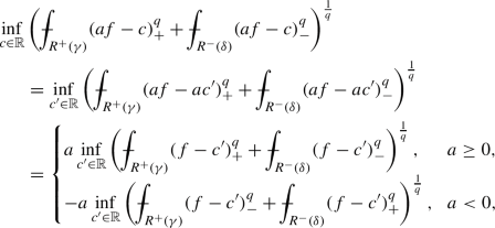

with \(c' =c/a\). The claim follows from this observation.
-
(iv)
For the positive part, we have
$$\begin{aligned}&\int _{R^+(\gamma )} (\max \{f,g\} - \max \{c_R^f,c_R^g\})_+^q \\&\qquad \le \int _{R^+(\gamma ) \cap \{ f \ge g \} } (\max \{f,g\} -c_R^f)_+^q + \int _{R^+(\gamma ) \cap \{ f< g \} } ( \max \{f,g\} -c_R^g)_+^q \\&\qquad = \int _{R^+(\gamma ) \cap \{ f \ge g \} } (f -c_R^f)_+^q + \int _{R^+(\gamma ) \cap \{ f < g \} } ( g -c_R^g)_+^q \\&\qquad \le \int _{R^+(\gamma ) } (f -c_R^f)_+^q + \int _{R^+(\gamma ) } ( g -c_R^g)_+^q . \end{aligned}$$
For the negative part, we have

Hence, we obtain

By taking supremum over all parabolic rectangles \(R \subset \Omega _T\), we conclude that
The claim for \(\min \{f,g\}\) follows similarly. \(\square \)
Remark 2.10
Every function \(f \in \mathrm {PBMO}_{\gamma ,\delta ,q}^{+}(\Omega _T)\) can be approximated pointwise by a sequence of bounded \(\mathrm {PBMO}_{\gamma ,\delta ,q}^{+}(\Omega _T)\) functions, since the truncations
belong to \(\mathrm {PBMO}_{\gamma ,\delta ,q}^{+}(\Omega _T)\) with
for every \(k\in \mathbb N\), see (i) and (iv) of Lemma 2.8, and it holds that \(f_k \rightarrow f\) pointwise and in \(L_{\mathrm {loc}}^q(\Omega _T)\) as \(k \rightarrow \infty \).
3 Parabolic John–Nirenberg inequalities
This section discusses several versions of the John–Nirenberg inequality for parabolic \(\mathrm {BMO}\). We begin with a version where the exponential bound is given in terms of integral averages. For short, we suppress the variables (x, t) in the notation and, for example, write
in the sequel.
Theorem 3.1
Let \(R \subset {\mathbb {R}}^{n+1}\) be a parabolic rectangle, \(0 \le \gamma < 1\), \(\gamma< \alpha < 1\) and \(0 < q \le 1\). Assume that \(f \in \mathrm {PBMO}_{\gamma ,q}^+(R)\) and let \(\left\Vert {f}\right\Vert =\left\Vert {f}\right\Vert _{\mathrm {PBMO}_{\gamma ,q}^{+}(R)}\). Then there exist constants \(c_R\in \mathbb R\), \(A=A(n,p,q,\gamma ,\alpha )\), \(B=B(n,p,q,\gamma ,\alpha )\) and \(C=C(n,p,q,\gamma ,\alpha )\) such that
and
for every \(\lambda \ge C \left\Vert {f}\right\Vert \).
Proof
Let \(R_0=R=R(x_0,t_0,L) = Q(x_0,L) \times (t_0-L^p, t_0+L^p)\). By considering the function \(f(x+x_0,t+t_0)\), we may assume that the center of \(R_0\) is the origin, that is, \(R_0 = Q(0,L) \times (-L^p, L^p)\). By (i) and (iii) of Lemma 2.8, we may assume that \(c_{R_0} = 0\) and \(\left\Vert {f}\right\Vert ^q = \tfrac{1}{2}(1-\alpha )/(1-\gamma )\). We note that it is sufficient to prove the first inequality of the theorem since the second inequality follows from the first one by applying it to the function \(-f(x,-t)\).
We claim that
for every \(\lambda \ge C \left\Vert {f}\right\Vert \). Let m be the smallest integer with \(3 + \alpha \le 2^{pm+1} (\alpha - \gamma )\), that is,
Let \(S^+_0 = R^+_0(\alpha ) = Q(0,L) \times (\alpha L^p,L^p) \). The time length of \(S^+_0\) is \(l_t(S^+_0) = (1-\alpha )L^p\). We partition \(S^+_0\) by dividing each spatial edge \([-L,L]\) into \(2^m\) equally long intervals. If
we divide the time interval of \(S^+_0\) into \(\lfloor 2^{pm} \rfloor \) equally long intervals. Otherwise, we divide the time interval of \(S^+_0\) into \(\lceil 2^{pm} \rceil \) equally long intervals. We obtain subrectangles \(S^+_1\) of \(S^+_0\) with spatial side length \(l_x(S^+_1)=l_x(S^+_0)/2^m = L / 2^m\) and time length either
For every \(S^+_1\), there exists a unique rectangle \(R_1\) with spatial side length \(l_x = L / 2^{m}\) and time length \(l_t = 2 L^p / 2^{mp}\) such that \(R_1\) has the same top as \(S^+_1\). We select those rectangles \(S^+_1\) for which \(\lambda < c_{R_1}\) and denote the obtained collection by \(\{ S^+_{1,j} \}_j\). If \(\lambda \ge c_{R_1}\), we subdivide \(S^+_1\) in the same manner as above and select all those subrectangles \(S^+_2\) for which \(\lambda < c_{R_2}\) to obtain family \(\{ S^+_{2,j} \}_j\). We continue this selection process recursively. At the ith step, we partition unselected rectangles \(S^+_{i-1}\) by dividing each spatial side into \(2^m\) equally long intervals. If
we divide the time interval of \(S^+_{i-1}\) into \(\lfloor 2^{pm} \rfloor \) equally long intervals. If
we divide the time interval of \(S^+_{i-1}\) into \(\lceil 2^{pm} \rceil \) equally long intervals. We obtain subrectangles \(S^+_i\). For every \(S^+_i\), there exists a unique rectangle \(R_i\) with spatial side length \(l_x = L / 2^{mi}\) and time length \(l_t = 2 L^p / 2^{pmi}\) such that \(R_i\) has the same top as \(S^+_i\). Select those \(S^+_i\) for which \(\lambda < c_{R_i}\) and denote the obtained collection by \(\{ S^+_{i,j} \}_j\). If \(\lambda \ge c_{R_i}\), we continue the selection process in \(S^+_i\). In this manner we obtain a collection \(\{S^+_{i,j} \}_{i,j}\) of pairwise disjoint rectangles.
Observe that if (3.1) holds, then we have
On the other hand, if (3.2) holds, then
This gives an upper bound
for every \(S_i^+\).
Suppose that (3.2) is satisfied at the ith step. Then we have a lower bound for the time length of \(S_i^+\), since
On the other hand, if (3.1) is satisfied, then
In this case, (3.2) has been satisfied at an earlier step \(i'\) with \(i'< i\). We obtain
by using the lower bound for \(S_{i'}^+\). Thus, we have
for every \(S^+_i\). By using the lower bound for the time length of \(S^+_i\) and the choice of m, we observe that
This implies
for a fixed rectangle \(S^+_{i-1}\) and for every subrectangle \(S^+_{i} \subset S^+_{i-1}\) (see Fig. 1). By the construction of the subrectangles \(S^+_i\), we have
and

Schematic picture of the decomposition at the ith step
We have a collection \(\{ S^+_{i,j} \}_{i,j}\) of pairwise disjoint rectangles. However, the rectangles in the corresponding collection \(\{ S^-_{i,j} \}_{i,j}\) may overlap. Thus, we replace it by a subfamily \(\{ \widetilde{S}^-_{i,j} \}_{i,j}\) of pairwise disjoint rectangles, which is constructed in the following way. At the first step, choose \(\{ S^-_{1,j} \}_{j}\) and denote it by \(\{ \widetilde{S}^-_{1,j} \}_j\). Then consider the collection \(\{ S^-_{2,j} \}_{j}\) where each \(S^-_{2,j}\) either intersects some \(\widetilde{S}^-_{1,j}\) or does not intersect any \(\widetilde{S}^-_{1,j}\). Select the rectangles \(S^-_{2,j}\) that do not intersect any \(\widetilde{S}^-_{1,j}\), and denote the obtained collection by \(\{ \widetilde{S}^-_{2,j} \}_j\). At the ith step, choose those \(S^-_{i,j}\) that do not intersect any previously selected \(\widetilde{S}^-_{i',j}\), \(i' < i\). Hence, we obtain a collection \(\{ \widetilde{S}^-_{i,j} \}_{i,j}\) of pairwise disjoint rectangles. Observe that for every \(S^-_{i,j}\) there exists \(\widetilde{S}^-_{i',j}\) with \(i' < i\) such that
Here pr\(_x\) denotes the projection to \(\mathbb R^n\) and pr\(_t\) denotes the projection to the time axis.
Rename \(\{ S^+_{i,j} \}_{i,j}\) and \(\{ \widetilde{S}^-_{i,j} \}_{i,j}\) as \(\{ S^+_{i} \}_{i}\) and \(\{ \widetilde{S}^-_{j} \}_j\), respectively. Let \(S(\lambda ) = \bigcup _i S^+_i\). Note that \(S^+_i\) is spatially contained in \(S^-_i\), that is, \(\text {pr}_x S^+_i\subset \text {pr}_x S^-_i\). In the time direction, we have
since
Therefore, by (3.6) and (3.7), it holds that
Let \(\lambda> \delta > 0\) and consider the collection \(\{S^+_k\}_k\) for \(\delta \). Then every \(S^+_i\) is contained in a unique \(S^+_k\). Let \({\mathcal {J}}_k = \{ j \in {\mathbb {N}}: \widetilde{S}^+_j \subset S^+_k \}\). Using (3.5), we have

for every \(\widetilde{S}^-_j\). By summing over j, we obtain
Let \(k \in {\mathbb {N}}\). We have \(\widetilde{S}^+_j \subset S^+_k\) for every \(j \in {\mathcal {J}}_k\), where \(S^+_k\) was obtained by subdividing a previous \(S^+_{k^-}\) for which \(a_{R_{k^-}} \le \delta \). Hence, it holds that \(\widetilde{S}^-_j \subset R_k\) for every \(j \in {\mathcal {J}}_k\). By (3.3), it follows that \(\widetilde{S}^-_j \subset R^+_{k^-}(\gamma )\) for every \(j \in {\mathcal {J}}_k\). Since \(\widetilde{S}^-_j\) are pairwise disjoint, by applying (3.4) together with (3.5), we arrive at
where
By summing over k and applying (3.9), we obtain
Thus, we have
for every \(\lambda ^q > \delta ^q + 1\). By (3.8), we obtain
for every \(\lambda ^q > \delta ^q + 1\). By setting \(a = 2c_1 c_2 + 1\) and replacing \(\lambda ^q\) and \(\delta ^q\) by \(\lambda + a\) and \(\lambda \), respectively, we have
Assume that \(\lambda \ge a\). Then there exists an integer \(N \in {\mathbb {Z}}_+\) such that \(Na \le \lambda < (N+1)a\). By iterating (3.10), we arrive at
Applying (3.8), (3.9) and (3.3), we get
This implies
for every \(\lambda \ge a^\frac{1}{q}\) with
If \((x,t) \in S^+_0 {\setminus } S(\lambda )\), then there exists a sequence \(\{S^+_l\}_{l\in \mathbb N}\) of subrectangles containing (x, t) such that \(c_{R_l} \le \lambda \) and \(|S^+_l |\rightarrow 0\) as \(l \rightarrow \infty \). This implies

The Lebesgue differentiation theorem (Lemma 2.3) implies that \(f(x,t)^q_+ \le 1 + \lambda ^q\) for almost every \((x,t) \in S^+_0 {\setminus } S(\lambda )\). It follows that
up to a set of measure zero. Given \(\lambda \ge 2^\frac{1}{q}\), we have \(\lambda ^q \ge 1 + \frac{\lambda ^q}{2} \). We conclude that
for every \(\lambda \ge (2 a)^\frac{1}{q} = \bigl (4a(1-\gamma )/(1-\alpha )\bigr )^\frac{1}{q} \left\Vert {f}\right\Vert = C \left\Vert {f}\right\Vert \). This completes the proof. \(\square \)
As a corollary of Theorem 3.1, we obtain a more standard version of the parabolic John–Nirenberg inequality.
Corollary 3.2
Let \(R \subset {\mathbb {R}}^{n+1}\) be a parabolic rectangle, \(0 \le \gamma < 1\), \(\gamma< \alpha < 1\) and \(0 < q \le 1\). Assume that \(f \in \mathrm {PBMO}_{\gamma ,q}^+(R)\) and let \(\left\Vert {f}\right\Vert =\left\Vert {f}\right\Vert _{\mathrm {PBMO}_{\gamma ,q}^{+}(R)}\). Then there exist constants \(c_{R}\in \mathbb R\), \(A=A(n,p,q,\gamma ,\alpha )\) and \(B=B(n,p,q,\gamma ,\alpha )\) such that
and
for every \(\lambda > 0\).
Proof
By Theorem 3.1, there exists a constant \(C=C(n,p,q,\gamma ,\alpha )\) such that
for every \(\lambda \ge C \left\Vert {f}\right\Vert \). On the other hand, if \(0<\lambda < C \left\Vert {f}\right\Vert \), then
This proves the first inequality in the theorem. The second inequality follows similarly. \(\square \)
Another consequence of Theorem 3.1 is a weak reverse Hölder inequality for parabolic \(\mathrm {BMO}\). In particular, this implies that a function in parabolic \(\mathrm {BMO}\) is locally integrable to any positive power.
Corollary 3.3
Let \(R \subset {\mathbb {R}}^{n+1}\) be a parabolic rectangle, \(0 \le \gamma < 1\), \(\gamma< \alpha < 1\), \(0 < q \le 1\) and \(q \le r < \infty \). Assume that \(f \in \mathrm {PBMO}_{\gamma ,q}^+(R)\) and let \(\left\Vert {f}\right\Vert =\left\Vert {f}\right\Vert _{\mathrm {PBMO}_{\gamma ,q}^{+}(R)}\). Then there exist constants \(c_{R}\in \mathbb R\) and \(c=c(n,p,q,r,\gamma ,\alpha )\) such that
and
Proof
Let
By using Cavalieri’s principle, we get
where \(C=C(n,p,q,\gamma ,\alpha )\) is the constant in Theorem 3.1. We estimate the obtained integrals separately. For \(0 \le \lambda \le C \left\Vert {f}\right\Vert \), we have \(\lambda ^{r-1} \le (C \left\Vert {f}\right\Vert )^{r-q} \lambda ^{q-1}\), and thus
For the second integral, we apply Theorem 3.1 to obtain
where we applied a change of variables \(s = B\lambda ^q/\left\Vert {f}\right\Vert ^q \). This implies
The second inequality of the theorem follows similarly. \(\square \)
4 Chaining arguments and the time lag
Applying Corollary 3.2 with chaining arguments, we obtain a parabolic John–Nirenberg inequality, which allows us to change the time lag.
Theorem 4.1
Let \(R \subset {\mathbb {R}}^{n+1}\) be a parabolic rectangle, \(0< \gamma <1\), \(-1 < \rho \le \gamma \), \(-\rho < \sigma \le \gamma \) and \(0<q \le 1\). Assume that \(f \in \mathrm {PBMO}_{\gamma ,q}^+(R)\) and let \(\left\Vert {f}\right\Vert =\left\Vert {f}\right\Vert _{\mathrm {PBMO}_{\gamma ,q}^{+}(R)}\). Then there exist constants \(c \in {\mathbb {R}}\), \(A=A(n,p,q,\gamma ,\rho ,\sigma )\) and \(B=B(n,p,q,\gamma ,\rho ,\sigma )\) such that
and
for every \(\lambda > 0\).
Proof
Let \(R_0 = R\). Without loss of generality, we may assume that the center of \(R_0\) is the origin. Since \(f \in \mathrm {PBMO}^+_{\gamma ,q}(R_0)\), Corollary 3.2 holds for any parabolic subrectangle of \(R_0\) and for any \(\gamma< \alpha <1\). Let m be the smallest integer with
Then there exists \(0 \le \varepsilon < 1\) such that
We partition \(R^+_0(\rho ) = Q(0, L) \times (\rho L^p, L^p)\) by dividing each of its spatial edges into \(2^m\) equally long intervals and the time interval into \(\lceil (1-\rho )2^{mp}/(1-\alpha )\rceil \) equally long intervals. Denote the obtained rectangles by \(U^+_{i,j}\) with \(i \in \{1,\dots ,2^{mn}\}\) and \(j \in \{1,\dots ,\lceil (1-\rho )2^{mp}/(1-\alpha )\rceil \}\). The spatial side length of \(U^+_{i,j}\) is \(l = l_x(U^+_{i,j}) =L/2^m\) and the time length is
For every \(U^+_{i,j}\), there exists a unique rectangle \(R_{i,j}\) that has the same top as \(U^+_{i,j}\). Our aim is to construct a chain from each \(U^+_{i,j}\) to a central rectangle which is of the same form as \(R_{i,j}\) and is contained in \(R_0\). This central rectangle will be specified later. First, we construct a chain with respect to the spatial variable. Fix \(U^+_{i,j}\). Let \(P_0 = R_{i,j}\) and
We construct a chain of cubes from \(Q_i\) to the central cube Q(0, l). Let \(Q'_0 = Q_i = Q(x_i, l)\) and set
where \(1 \le \theta \le \sqrt{n}\) depends on the angle between \(x_i\) and the spatial axes and is chosen such that the center of \(Q_k\) is on the boundary of \(Q_{k-1}\) (see Fig. 2). We have
and \(\left|{x_i}\right| = \frac{\theta }{2} (L - bl)\), where \(b \in \{1, \dots , 2^m\}\) depends on the distance of \(Q_i\) to the center of \(Q_0 = Q(0,L)\). The number of cubes in the spatial chain \(\{Q'_k\}_{k=0}^{N_i}\) is

Sketch of a spatial chain of cubes \(Q'_k\)
Next, we also take the time variable into consideration in the construction of the chain. Let
and \(P^-_k = P^+_k - (0, (1+\alpha )l^p)\), for \(k \in \{ 0, \dots , N_i \}\), be the upper and the lower parts of a parabolic rectangle respectively. These will form a chain of parabolic rectangles from \(U^+_{i,j}\) to the eventual central rectangle. Observe that every rectangle \(P_{N_i}\) coincides spatially for all pairs (i, j). Consider \(j=1\) and such i that the boundary of \(Q_i\) intersects the boundary of \(Q_0\). For such a cube \(Q_i\), we have \(b=1\), and thus \(N = N_i = \frac{L}{l} - 1\). In the time variable, we travel from \(t_1\) the distance
We show that the lower part of the final rectangle \(P^-_N\) is contained in \(R_0\). To this end, we subtract the time length of \(U^+_{i,1}\) from the distance above and observe that it is less than half of the time length of \(R_0 {\setminus }(R_0^+(\rho ) \cup R_0^-(\sigma ))\). This follows from the computation
since
This implies that \(P^-_N \subset R_0^+(\rho - (\rho +\sigma )/2)\). Denote this rectangle \(P_N\) by \(\mathfrak {R} = \mathfrak {R}_\rho \). This is the central rectangle where all chains will eventually end.
Let \(j=1\) and assume that i is arbitrary. We extend the chain \(\{P_k\}_{k=0}^{N_i}\) by \(N - N_i\) rectangles into the negative time direction such that the final rectangle coincides with the central rectangle \(\mathfrak {R}\) (see Fig. 3a). More precisely, we consider \(Q'_{k+1} = Q'_{N_i}\),
for \(k \in \{N_i, \dots , N-1\}\). For every \(j \in \{2,\dots ,\lceil (1-\rho )2^{mp}/(1-\alpha )\rceil \}\), we consider a similar extension of the chain. The final rectangles of the chains coincide for fixed j and for every i. Moreover, every chain is of the same length \(N+1\), and it holds that

Schematic pictures of constructed chains
Then we consider an index \(j \in \{2,\dots ,\lceil (1-\rho )2^{mp}/(1-\alpha )\rceil \}\) related to the time variable. The time distance between the current ends of the chains for pairs (i, j) and (i, 1) is
Our objective is to have the final rectangle of the continued chain for (i, j) to coincide with the end of the chain for (i, 1), that is, with the central rectangle \(\mathfrak {R}\). To achieve this, we modify \(2^{m-1}\) intersections of \(P^+_k\) and \(P^-_{k+1}\) by shifting \(P_k\) and also add a chain of \(M_j\) rectangles traveling to the negative time direction into the chain \(\{P_k\}_{k=0}^{N}\). We shift every \(P_k, k \in \{ 1, \dots , 2^{m-1} \}\), by a \(\beta _j\)-portion of their temporal length more than the previous rectangle was shifted, that is, we move each \(P_k\) into the negative time direction a distance of \(k \beta _j (1-\alpha ) l^p\) (see Fig. 3b). The values of \(M_j \in {\mathbb {N}}\) and \(0\le \beta _j <1\) will be chosen later. In other words, modify the definitions of \(P^+_k\) for \( k \in \{ 1, \dots , 2^{m-1} \}\) by
and then add \(M_j\) rectangles defined by
for \(k \in \{N,\dots , N+M_j-1\}\). Note that there exists \(1 \le \tau < 2\) such that
We would like to find such \(0\le \beta _j <1\) and \(M_j \in {\mathbb {N}}\) that
which is equivalent with
With this choice all final rectangles coincide. Choose \(M_j \in {\mathbb {N}}\) such that
that is,
and
By choosing \(0\le \beta _j <1\) such that
we have
Observe that \(0\le \beta _j \le \frac{1}{2}\) for every j. For measures of the intersections of the modified rectangles, it holds that
for \( k \in \{ 1, \dots , 2^{m-1} \}\), and thus
for every \(k \in \{1,\dots , N+M_j\}\). Fix \(U^+_{i,j}\). We conclude that

where
for every j. Hence, we obtain
We observe that
The first sum of the right-hand side can be estimated by Corollary 3.2 as follows
To estimate the second sum above, assume that \(\lambda \ge 2 C \left\Vert {f}\right\Vert \). This implies that
for every i, j. Thus
for every \(\lambda \ge 2 C \left\Vert {f}\right\Vert \). For \(0<\lambda < 2 C \left\Vert {f}\right\Vert \), we have
We can apply a similar chaining argument in the reverse time direction for \(R_0^-(\sigma )\) with the exception that we also extend (and modify if needed) every chain such that the central rectangle \(\mathfrak {R}_\sigma \) coincides with \(\mathfrak {R}=\mathfrak {R}_\rho \). A rough upper bound for the number of rectangles needed for the additional extension is given by
Thus, the constant C above is two times larger in this case. This proves the second inequality of the theorem. \(\square \)
The next corollary of Theorem 4.1 tells that the spaces \(\mathrm {PBMO}_{\gamma ,\delta ,q}^{+}\) coincide for every \(-1<\gamma <1\), \(-\gamma< \delta <1\) and \(0<q<\infty \).
Corollary 4.2
Let \(\Omega _T \subset {\mathbb {R}}^{n+1}\) be a space-time cylinder, \(0<\gamma <1\), \(-1 < \rho \le \gamma \), \(-\rho < \sigma \le \gamma \) and \(0<q \le r<\infty \). Then there exist constants \(c_1=c_1(n,p,q,r,\gamma ,\rho ,\sigma )\) and \(c_2=c_2(n,p,q,r,\gamma ,\rho ,\sigma )\) such that
Proof
Let R be a parabolic subrectangle of \(\Omega _T\). By Hölder’s inequality, we have

where \(c_0 = \max \{1, 2^{\frac{1}{q}-1} \} \max \{1, 2^{1 -\frac{1}{r}} \}\). We observe that

By taking supremum over all parabolic subrectangles \(R \subset \Omega _T\), we arrive at
To show the second inequality, we make the restriction \(0 < q \le 1\) so that we can apply Theorem 4.1. This is not an issue since after establishing the second inequality for \(0 < q \le 1\) we can use the first inequality to obtain the whole range \(0 < q \le r\). Cavalieri’s principle and Theorem 4.1 imply that

where we applied a change of variables \(s = B\lambda ^q\left\Vert {f}\right\Vert _{\mathrm {PBMO}_{\gamma ,q}^{+}(R)}^{-q}\). Similarly, we obtain

By adding up the two estimates above and taking supremum over all parabolic rectangles \(R \subset \Omega _T\), we conclude that
\(\square \)
5 A global parabolic John–Nirenberg inequality
The results in the previous sections are local in the sense that they give estimates on a parabolic rectangle \(R\subset \Omega _T\). Next we discuss the corresponding estimates on the entire domain under the assumption that the domain \(\Omega \subset \mathbb R^n\) satisfies a quasihyperbolic boundary condition.
Definition 5.1
The quasihyperbolic metric in a domain \(\Omega \subset {\mathbb {R}}^n\) is defined by setting, for any \(x_1,x_2\in \Omega \),
where the infimum is taken over all rectifiable paths \(\gamma _{x_1x_2}\) in \(\Omega \) connecting \(x_1\) to \(x_2\).
Definition 5.2
A domain \(\Omega \) is said to satisfy the quasihyperbolic boundary condition if there exist \(x_0 \in \Omega \) and constants \(c_1\) and \(c_2\) such that
for every \(x \in \Omega \).
The class of the domains satisfying the quasihyperbolic boundary condition was first introduced in [7]. Note that a domain satisfying the quasihyperbolic boundary condition is bounded. In [22], a parabolic John–Nirenberg lemma was proven for domains satisfying the quasihyperbolic boundary condition. We state it here in its complete form.
Theorem 5.3
Assume that \(\Omega \subset {\mathbb {R}}^n\) satisfies the quasihyperbolic boundary condition. Let \(0< \gamma <1\), \(0<q \le 1\) and \(0< \tau _1< \tau _2 < T\). Assume that \(f\in \mathrm {PBMO}^+_{\gamma ,q}(\Omega _T)\) and let \(\left\Vert {f}\right\Vert = \left\Vert {f}\right\Vert _{\mathrm {PBMO}_{\gamma ,q}^{+}(\Omega _T)}\). Then there exist constants \(c \in {\mathbb {R}}\), \(A=A(n,p,q,\gamma ,\Omega ,\tau _1,\tau _2)\) and \(B=B(n,p,q,\gamma ,\Omega ,\tau _1,\tau _2)\) such that
and
for every \(\lambda > 0\).
As a corollary of Theorem 5.3, the positive part of a PBMO\(^{+}\) function is exponentially integrable on upper parts of space-time cylinders and the negative part on lower parts.
Corollary 5.4
Assume that \(\Omega \subset {\mathbb {R}}^n\) satisfies the quasihyperbolic boundary condition and let \(0< \tau _1< \tau _2 < T\). Assume that \(f\in \mathrm {PBMO}^+(\Omega _T)\) and let \(\left\Vert {f}\right\Vert = \left\Vert {f}\right\Vert _{\mathrm {PBMO}^{+}(\Omega _T)}\). If \(0<\delta <B/\left\Vert {f}\right\Vert \), then

where B and c are the constants from Theorem 5.3.
Proof
Let \(E = \Omega \times (\tau _2,T)\). Cavalieri’s principle and Theorem 5.3 with \(q=1\) imply
Here we applied a change of variables \(\lambda = e^s\). The second inequality follows in a similar way. \(\square \)
The following theorem gives the characterization of the domains on which the parabolic John–Nirenberg lemma holds globally.
Theorem 5.5
Let \(0< \tau _1< \tau _2 < T\). A domain \(\Omega \) satisfies the quasihyperbolic boundary condition if and only if there exist \(\delta > 0\) and \(c\in {\mathbb {R}}\) such that

for every \(f \in \mathrm {PBMO}^+(\Omega _T)\) with \(\left\Vert {f}\right\Vert = \left\Vert {f}\right\Vert _{\mathrm {PBMO}^{+}(\Omega _T)}\).
Proof
One direction follows from the proof of Corollary 5.4 by choosing \(0<\delta \le \tfrac{B}{1+A} \frac{1}{\left\Vert {f}\right\Vert }\). For the other direction, we consider \(f(x,t) = k(x_0,x)\), where \(k(x_0,x)\) denotes the quasihyperbolic metric in \(\Omega \). We note that
By [24, Theorem A], we conclude that \(f \in \mathrm {BMO}(\Omega )\). Thus, we have \(f \in \mathrm {PBMO}^+(\Omega _T)\) and the parabolic John–Nirenberg inequality of the claim applies for f. Set \(\tilde{\delta } =\delta /4\). By applying Jensen’s inequality twice, Young’s inequality and the parabolic John–Nirenberg inequality, we obtain

By [24, Theorem A], the domain \(\Omega \) satisfies the quasihyperbolic boundary condition. \(\square \)
6 Parabolic \(\mathrm {BMO}\) with medians
This section discusses John–Nirenberg inequalities for the median-type parabolic \(\mathrm {BMO}\). In many cases, it is preferable to consider medians instead of integral averages. Let \(0<s \le 1\). Assume that \(E \subset {\mathbb {R}}^{n+1}\) is a measurable set with \(0<|E|<\infty \) and that \(f:E\rightarrow [-\infty , \infty ]\) is a measurable function. A number \(a\in \mathbb R\) is called an s-median of f over E, if
In general, the s-median is not unique. To obtain a uniquely defined notion, we consider the maximal s-median as in [21].
Definition 6.1
Let \(0<s \le 1\). Assume that \(E \subset {\mathbb {R}}^{n+1}\) is a measurable set with \(0<|E|<\infty \) and that \(f:E\rightarrow [-\infty , \infty ]\) is a measurable function. The maximal s-median of f over E is defined as
The maximal s-median of a function is an s-median [21]. In the next lemma, we list the basic properties of the maximal s-median. We refer to [20, 21] for the proofs of the properties.
Lemma 6.2
Let \(0<s \le 1\). Assume that \(E \subset {\mathbb {R}}^{n+1}\) is a measurable set with \(0<|E|<\infty \) and that \(f,g:E\rightarrow [-\infty , \infty ]\) are measurable functions. The maximal s-median has the following properties.
-
(i)
\(m_f^{s'}(E) \le m_f^s(E)\) for any \(0<s \le s'\le 1\).
-
(ii)
\(m_f^s(E) \le m_g^s(E)\) whenever \(f\le g\) almost everywhere in E.
-
(iii)
If \(E \subset E'\) and \(|E'| \le c |E|\) with some \(c \ge 1\), then \(m_f^s(E) \le m_f^{s/c}(E')\).
-
(iv)
\(m_{\varphi \circ f}^s(E) = \varphi (m_f^s(E))\) for an increasing continuous function \(\varphi : f(E) \rightarrow [-\infty , \infty ]\).
-
(v)
\(m_f^s(E) + c = m_{f+c}^s(E)\) for any \(c \in {\mathbb {R}}\).
-
(vi)
\(m_{cf}^s(E) = c \, m_f^s(E)\) for any \(c > 0\).
-
(vii)
\(|m_{f}^s(E)| \le m_{|f|}^{\min \{s,1-s\}}(E)\).
-
(viii)
\(m_{f+g}^s(E) \le m_f^{t_1}(E) + m_g^{t_2}(E)\) whenever \(t_1 + t_2 \le s\).
-
(ix)
For any \(f \in L^p(E)\) with \(p>0\),
-
(x)
If \(E_i\), \(i \in {\mathbb {N}}\), are pairwise disjoint measurable sets, then
$$\begin{aligned} \inf _{i} m_f^s(E_i) \le m_f^s\Bigl (\bigcup _{i=1}^\infty E_i\Bigr ) \le \sup _{i} m_f^s(E_i) . \end{aligned}$$

Lemma 2.3 can be combined with the proof of the Lebesgue differentiation theorem for medians in [21] to obtain the following lemma.
Lemma 6.3
Let \(f: {\mathbb {R}}^{n+1} \rightarrow [-\infty , \infty ]\) be a measurable function which is finite almost everywhere in \(\mathbb R^{n+1}\) and \(0<s\le 1\). Then
for almost every \((x,t) \in {\mathbb {R}}^{n+1}\), whenever \((A_i)_{i\in \mathbb N}\) is a sequence of measurable sets converging regularly to (x, t).
Definition 6.4
Let \(\Omega \subset {\mathbb {R}}^n\) be a domain and \(T>0\). Given \(0 \le \gamma < 1\) and \(0<s \le 1\), we say that a measurable function \(f:\Omega _T\rightarrow [-\infty ,\infty ]\) belongs to the median-type parabolic \(\mathrm {BMO}\), denoted by \(\mathrm {PBMO}_{\gamma ,0,s}^{+}(\Omega _T)\), if
If the condition above holds with the time axis reversed, then \(f \in \mathrm {PBMO}_{\gamma ,0,s}^{-}(\Omega _T)\).
The next lemma is a counterpart of Lemma 2.7. The proof is similar to that of Lemma 2.7 and thus is omitted here.
Lemma 6.5
Let \(\Omega _T \subset {\mathbb {R}}^{n+1}\) be a space-time cylinder, \(0 \le \gamma < 1\) and \(0<s \le 1\). Assume that \(f:\Omega _T\rightarrow [-\infty ,\infty ]\) is a measurable function. Then for every parabolic rectangle \(R\subset \Omega _T\), there exists a constant \(c_R\in \mathbb R\), that may depend on R, such that
In particular,
The following John–Nirenberg lemma is a counterpart of Corollary 3.2. We apply the same decomposition argument as in the proof of Theorem 3.1.
Theorem 6.6
Let \(R \subset {\mathbb {R}}^{n+1}\) be a parabolic rectangle, \(0 \le \gamma < 1\), \(\gamma< \alpha < 1\) and \(0 < s \le s_0\), where \(s_0\) is a small positive number. Assume that \(f \in \mathrm {PBMO}_{\gamma ,0,s}^+(R)\) and let \(\left\Vert {f}\right\Vert = \left\Vert {f}\right\Vert _{\mathrm {PBMO}_{\gamma ,0,s}^{+}(R)}\). Then there exist constants \(c_R\in \mathbb R\), \(A=A(n,p,\gamma ,\alpha )\) and \(B=B(n,p,\gamma ,\alpha )\) such that
and
for every \(\lambda > 0\).
Proof
We use the same notation as in the proof of Theorem 3.1 until Eq. (3.8) with the exception that we assume \(\left\Vert {f}\right\Vert = 1\). We proceed from there. It holds that
where \(c_1 = 3(7+\alpha )/(1-\alpha )\). Take \(\lambda> \delta > 0\) and form \(\{S^+_k\}_k\) for \(\delta \). Each \(S^+_i\) is contained in a unique \(S^+_k\). Set \({\mathcal {J}}_k = \{ j: \widetilde{S}^+_j \subset S^+_k \}\) and define
By using properties (viii) and (iii) of Lemma 6.2 together with (3.5), we obtain
for every \(\widetilde{S}^-_j\), where \(r=1 - 2s(1-\gamma )/(1-\alpha )\). Since \(\widetilde{S}^-_j\) are pairwise disjoint for \(j \in {\mathcal {J}}_k\), property (x) of Lemma 6.2 implies that
for every \(k \in {\mathbb {N}}\).
Fix \(k \in {\mathcal {K}}\). We have \(\widetilde{S}^+_j \subset S^+_k\) for all \(j \in {\mathcal {J}}_k\), where \(S^+_k\) was obtained by subdividing a previous \(S^+_{k^-}\) for which \(a_{R_{k^-}} \le \delta \). Hence, it holds that \(\widetilde{S}^-_j \subset R_k\) for all \(j \in {\mathcal {J}}_k\). By (3.3), it follows that \(\widetilde{S}^-_j \subset R^+_{k^-}(\gamma )\) for every \(j \in {\mathcal {J}}_k\) and thus also \(\bigcup _{j \in {\mathcal {J}}_k} \widetilde{S}^-_j \subset R^+_{k^-}(\gamma )\). Using (3.4) and (3.5), we get
for every \(k \in {\mathcal {K}}\), where
By applying (iii), (ii) and (v) of Lemma 6.2, we have
for \(k \in {\mathcal {K}}\), where \({\tilde{c}} = 2 c_1 c_2\) and whenever \(s \le r / {\tilde{c}}\). By combining estimates (6.2) and (6.3), we obtain
for \(k \in {\mathcal {K}}\). Thus, whenever \(\lambda > \delta + 1\), we have
On the other hand, if \(k \notin {\mathcal {K}}\), we have
which implies
By combining the cases \(k \in {\mathcal {K}}\) and \(k \notin {\mathcal {K}}\), we obtain
whenever \(\lambda > \delta + 1\). Applying (6.1), we arrive at
whenever \(\lambda > \delta + 1\). Set \(a = 2c_1 c_2 + 1\) and replace \(\lambda \) and \(\delta \) by \(\lambda + a\) and \(\lambda \), respectively. We have
Assume that \(\lambda \ge a\). Then there exists an integer \(N \in {\mathbb {Z}}_+\) such that \(Na \le \lambda < (N+1)a\). A recursive application of (6.4) gives
Hence, we have
for \(\lambda \ge a\), where \(A=4\) and \(B = \frac{1}{2} \log 2/(2 c_1 c_2 + 1)\).
If \((x,t) \in S^+_0 {\setminus } S(\lambda )\), then there exists a sequence \(\{S^+_l\}_{l\in \mathbb N}\) of subrectangles containing (x, t) such that \(c_{R_l} \le \lambda \) and \(|S^+_l |\rightarrow 0\) as \(l \rightarrow \infty \). By (ii) and (v) of Lemma 6.2, we have
Lemma 6.3 then further implies that \(f(x,t)_+ \le 1 + \lambda \) for almost every \((x,t) \in S^+_0 {\setminus } S(\lambda )\). It follows that
up to a set of measure zero. For \(\lambda \ge 2\), we have \(\lambda \ge 1 + \frac{\lambda }{2}\). We conclude that
for every \(\lambda \ge 2a\). If \(0<\lambda < 2a\), the claim follows from the estimate
Finally, we discuss the restriction on the median level parameter s,
The proof is complete. \(\square \)
The following John–Nirenberg inequality is an analogy of Theorem 4.1 and its proof uses the same chaining argument.
Theorem 6.7
Let \(R \subset {\mathbb {R}}^{n+1}\) be a parabolic rectangle, \(0< \gamma <1\), \(-1 < \rho \le \gamma \), \(-\rho < \sigma \le \gamma \) and \(0<s \le s_0\). Assume that \(f \in \mathrm {PBMO}_{\gamma ,0,s}^+(R)\) and let \(\left\Vert {f}\right\Vert = \left\Vert {f}\right\Vert _{\mathrm {PBMO}_{\gamma ,0,s}^{+}(R)}\). Then there exist constants \(c \in {\mathbb {R}}\), \(A=A(n,p,\gamma ,\rho ,\sigma )\) and \(B=B(n,p,\gamma ,\rho ,\sigma )\) such that
and
for every \(\lambda > 0\).
Proof
We use the same notation as in the proof of Theorem 4.1 until the point where \((c_{R_{i,j}} - c_{\mathfrak {R}} )^q_+\) is estimated. By (v), (viii), (iii) and (i) of Lemma 6.2 in this order, we obtain
whenever \(s \le 1/2^{n+2}\). This is satisfied by the assumption \(s \le s_0\). We observe that
for every j. Hence, it holds that \((c_{R_{i,j}} - c_{\mathfrak {R}} )_+ \le C \left\Vert {f}\right\Vert \). The proof now proceeds in the exactly same way as in Theorem 4.1 except applying Theorem 6.6 instead of Corollary 3.2. Thus, we can stop here. \(\square \)
As a corollary of Theorem 6.7, the median-type parabolic \(\mathrm {BMO}\) coincides with the classical integral-type parabolic \(\mathrm {BMO}\), compare with Corollary 4.2. In particular, it follows that all results for the integral-type parabolic \(\mathrm {BMO}\) also hold for the median-type parabolic \(\mathrm {BMO}\) and vice versa.
Corollary 6.8
Let \(\Omega _T \subset {\mathbb {R}}^{n+1}\) be a space-time cylinder, \(0< \gamma <1\), \(0<q<\infty \), \(0< \rho < 1\) and \(0 < s \le s_0 \). Then there exist constants \(c_1=c_1(n,p,q,\gamma ,\rho ,s)\) and \(c_2=c_2(n,p,q,\gamma ,\rho ,s)\) such that
Proof
Fix \(0< \gamma < 1\) and assume that \(0 < \rho \le \gamma \). Let R be a parabolic subrectangle of \(\Omega _T\). By Lemma 6.2 (ix), we have

where \(c_0 = s^{-\frac{1}{q}} \max \{1, 2^{1 -\frac{1}{q}} \}\). We observe that

Taking supremum over all parabolic subrectangles \(R \subset \Omega _T\), we obtain
for \(0 < \rho \le \gamma \).
For the second inequality, Cavalieri’s principle and Theorem 6.7 imply that

where we made a change of variables \(s = B\lambda /\left\Vert {f}\right\Vert _{\mathrm {PBMO}_{\gamma ,0,s}^{+}(R)}\). Similarly, we obtain

By summing the two estimates above and taking supremum over all parabolic rectangles \(R \subset \Omega _T\), we get
for \(0 < \rho \le \gamma \). Applying Corollary 4.2, we obtain the claim for the whole range \(0< \rho < 1\). \(\square \)
References
Aimar, H.: Elliptic and parabolic BMO and Harnack’s inequality. Trans. Am. Math. Soc. 306(1), 265–276 (1988)
Berkovits, L.: Parabolic Muckenhoupt weights in the Euclidean space. J. Math. Anal. Appl. 379(2), 524–537 (2011)
Berkovits, L.: Parabolic John–Nirenberg spaces. J. Funct. Spaces Appl. 2012, 901917, 9 (2012)
Bögelein, V., Duzaar, F., Liao, N.: On the Hölder regularity of signed solutions to a doubly nonlinear equation. J. Funct. Anal. 281(9), 109173 (2021)
Bögelein, V., Duzaar, F., Kinnunen, J., Scheven, C.: Higher integrability for doubly nonlinear parabolic systems. J. Math. Pures Appl. (9) 143, 31–72 (2021)
Fabes, E.B., Garofalo, N.: Parabolic B.M.O. and Harnack’s inequality. Proc. Am. Math. Soc. 95(1), 63–69 (1985)
Gehring, F.W., Martio, O.: Lipschitz classes and quasiconformal mappings. Ann. Acad. Sci. Fenn. Ser. A I Math. 10, 203–219 (1985)
Gianazza, U., Vespri, V.: A Harnack inequality for solutions of doubly nonlinear parabolic equations. J. Appl. Funct. Anal. 1(3), 271–284 (2006)
Jawerth, B., Torchinsky, A.: Local sharp maximal functions. J. Approx. Theory 43(3), 231–270 (1985)
John, F.: Quasi-isometric mappings, Seminari 1962/63 Anal. Alg. Geom. e Topol., vol. 2, Ist. Naz. Alta Mat, Ediz. Cremonese, Rome, pp. 462–473 (1965)
John, F., Nirenberg, L.: On functions of bounded mean oscillation. Commun. Pure Appl. Math. 14, 415–426 (1961)
Kinnunen, J., Kuusi, T.: Local behaviour of solutions to doubly nonlinear parabolic equations. Math. Ann. 337(3), 705–728 (2007)
Kinnunen, J., Saari, O.: On weights satisfying parabolic Muckenhoupt conditions. Nonlinear Anal. 131, 289–299 (2016)
Kinnunen, J., Saari, O.: Parabolic weighted norm inequalities and partial differential equations. Anal. PDE 9(7), 1711–1736 (2016)
Kuusi, T., Siljander, J., Urbano, J.M.: Local Hölder continuity for doubly nonlinear parabolic equations. Indiana Univ. Math. J. 61(1), 399–430 (2012)
Kuusi, T., Laleoglu, R., Siljander, J., Urbano, J.M.: Hölder continuity for Trudinger’s equation in measure spaces. Calc. Var. Partial Differ. Equ. 54(1–2), 193–229 (2012)
Martín-Reyes, F.J., de la Torre, A.: One-sided BMO spaces. J. London Math. Soc. (2) 49(3), 529–542 (1994)
Moser, J.: A Harnack inequality for parabolic differential equations. Commun. Pure Appl. Math. 17, 101–134 (1964)
Moser, J.: Correction to: “A Harnack inequality for parabolic differential equations". Commun. Pure Appl. Math. 20, 231–236 (1967)
Myyryläinen, K.: Median-type John–Nirenberg space in metric measure spaces. J. Geom. Anal. 32(4), 131 (2022)
Poelhuis, J., Torchinsky, A.: Medians, continuity, and vanishing oscillation. Studia Math. 213(3), 227–242 (2012)
Saari, O.: Parabolic BMO and global integrability of supersolutions to doubly nonlinear parabolic equations. Rev. Mat. Iberoam. 32(3), 1001–1018 (2016)
Saari, O.: Parabolic BMO and the forward-in-time maximal operator. Ann. Mat. Pura Appl. (4) 197(5), 1477–1497 (2018)
Smith, W.: Exponential integrability of the quasi-hyperbolic metric on Hölder domains. Ann. Acad. Sci. Fenn. Ser. A I Math. 16(2), 345–360 (1991)
Strömberg, J.-O.: Bounded mean oscillation with Orlicz norms and duality of Hardy spaces. Indiana Univ. Math. J. 28(3), 511–544 (1979)
Trudinger, N.S.: Pointwise estimates and quasilinear parabolic equations. Commun. Pure Appl. Math. 189, 205–226 (1968)
Acknowledgements
The research was supported by the Academy of Finland, the National Key Research and Development Program of China (Grant No. 2020YFA0712900) and the National Natural Science Foundation of China (Grant Nos. 11971058 and 12071197).
Funding
Open Access funding provided by Aalto University.
Author information
Authors and Affiliations
Corresponding author
Ethics declarations
Conflict of interest
The authors declare that they have no conflict of interest.
Additional information
Publisher's Note
Springer Nature remains neutral with regard to jurisdictional claims in published maps and institutional affiliations.
Rights and permissions
Open Access This article is licensed under a Creative Commons Attribution 4.0 International License, which permits use, sharing, adaptation, distribution and reproduction in any medium or format, as long as you give appropriate credit to the original author(s) and the source, provide a link to the Creative Commons licence, and indicate if changes were made. The images or other third party material in this article are included in the article’s Creative Commons licence, unless indicated otherwise in a credit line to the material. If material is not included in the article’s Creative Commons licence and your intended use is not permitted by statutory regulation or exceeds the permitted use, you will need to obtain permission directly from the copyright holder. To view a copy of this licence, visit http://creativecommons.org/licenses/by/4.0/.
About this article

Cite this article
Kinnunen, J., Myyryläinen, K. & Yang, D. John–Nirenberg inequalities for parabolic BMO. Math. Ann. 387, 1125–1162 (2023). https://doi.org/10.1007/s00208-022-02480-y
Received:
Revised:
Accepted:
Published:
Issue Date:
DOI: https://doi.org/10.1007/s00208-022-02480-y