
Abstract
Random noncommutative geometry can be seen as a Euclidean path-integral quantization approach to the theory defined by the Spectral Action in noncommutative geometry (NCG). With the aim of investigating phase transitions in random NCG of arbitrary dimension, we study the nonperturbative Functional Renormalization Group for multimatrix models whose action consists of noncommutative polynomials in Hermitian and anti-Hermitian matrices. Such structure is dictated by the Spectral Action for the Dirac operator in Barrett’s spectral triple formulation of fuzzy spaces. The present mathematically rigorous treatment puts forward “coordinate-free” language that might be useful also elsewhere, all the more so because our approach holds for general multimatrix models. The toolkit is a noncommutative calculus on the free algebra that allows to describe the generator of the renormalization group flow—a noncommutative Laplacian introduced here—in terms of Voiculescu’s cyclic gradient and Rota–Sagan–Stein noncommutative derivative. We explore the algebraic structure of the Functional Renormalization Group equation and, as an application of this formalism, we find the \(\beta \)-functions, identify the fixed points in the large-N limit and obtain the critical exponents of two-dimensional geometries in two different signatures.
1 Introduction
Random Noncommutative Geometry (NCG), initiated by Barrett and Glaser [11], is a path-integral approach to the quantization of noncommutative geometries. This problem is mathematically interesting [20, Sect. 18.4] and has already been addressed by diverse methods in [18, 28, 57]. Also in physics, a satisfactory answer would shed light on the quantum structure of spacetime from a different angle. Namely, what seems to individuate a formulation of quantum of gravity in terms of NCG-structures is that these provide a natural language to treat both pure gravity and gravity coupled with matter at a geometrically indistinguishable footing. This holds for (the classical theory of) established matter sectors like the Standard Model [7, 17] and some theories beyond it [21].
Although the last point evokes rather the mathematical elegance of the NCG-applications, also from a pragmatic viewpoint it is important to stress that the search for a quantum theory of gravity that is capable of incorporating matter is of physical relevance: “matter matters” reads for instance in the asymptotically safe road to quantum gravity [24] (see also [67]). Indeed, a quick argument [31] based on the Renormalization Group (RG) discloses the mutual importance of each sector to the other, concretely
-
gravity loops like
 appear and influence matter and
 -
in a similar way, matter modifies the gravity sector

 appear and influence matter and
in the RG-flow. This suggests that both ought to be simultaneously treated and motivates us to develop, as a first step, the Functional Renormalization Group in random NCG, where potentially both sectors might harmonically coexist.
The Functional Renormalization Group Equation (FRGE; see the comprehensive up-to-date review [23]) is a modern framework describing the Wilsonian RG-flow [78] that governs the change of a quantum theory with scale. From the technical viewpoint, in order to determine the effective action, the FRGE—derived by Wetterich and Morris [55, 77]—offers an alternative to path-integration by replacing that task with a differential equation.
In this paper, the model of space(time) we focus on is an abstraction of fuzzy spaces [27, 30, 71], whose elements were later assembled into a spectral triple (the spin geometry object in NCG) called fuzzy geometry [8, 12]. For the future, in a broader NCG context, it would be desirable to relate the FRGE to the newly investigated truncations in the spectral NCG formalism [22, 42, 43] (see [29] for a preceding related idea), but for initial investigations fuzzy geometries are interesting enough and also in line with them, e.g., for the case of the sphere [76, Sect. 3.3].
One particular advantage of a fuzzy geometry being a spectral triple is the contact with Connes’ NCG formalism, in particular, the ability to encode the geometry in a (Dirac) operator D that serves as path integration variable in the quantum theory. Since fuzzy geometries are finite-dimensional, one can provide a mathematically precise definition of the partition function \({\mathcal {Z}}= \int _{\text {}} \mathrm {e}^{-\mathrm{Tr}f(D)} \mathrm {d}D\) that corresponds to the Spectral Action \(\mathrm{Tr}f(D)\), as far as f is a polynomial, in contrast to the bump function f used originally by Connes–Chamseddine [16]. In fact, this way to quantize fuzzy geometries was shown [8, 11] to lead to a certain class of multimatrix models further characterized in [61].
On the physics side, finite-dimensionality should not be seen as a shortage, as this dimension is related to energy or spatial resolution; in fact, rather it is in line with the existence of a minimal or Planck’s length. This is intuitively clear for the fuzzy sphere [41] on which—being spanned by finitely many spherical harmonics—it is impossible to separate (i.e. to measure) points lying arbitrarily near.
This discrete-dual picture (Fig. 1) can be interpreted as a pre-geometric phase, analogous to having simplices as building blocks of spacetime in discrete approaches to quantum gravity as Group Field Theory [9], Matrix Models [25, 38] or Tensor Models [46]. For those theories, but also for other approaches (e.g., Causal Dynamical Triangulations [2]), it is important [1, 26, 34, 36, 65] to explore phase transition to a manifold-like phase; in analogous way, the study of a condensation of fuzzy geometries to a continuum is physically relevant [40] (also addressed analytically in dimension-1 by [49]). With this picture in mind, we estimate here candidates for such phase transition.

A caricature of selected algebra elements of the fuzzy sphere. The real part of spherical harmonics \(Y^{m=\ell /2}_{\ell }\) for \(\ell =4,10,20,40\)
The largest part of this paper develops the mathematical formalism that allows such exploration. On top of well-known quantum field theory (QFT) techniques, the nonstandard results this paper bases on can be divided into three classes:
-
The models are originated in Random NCG [11]. Barrett’s characterization of Dirac operators makes contact with certain kind of multimatrix models [8]. Their Spectral Action was systematically computed in [61], organized by chord diagrams, which reappear here.
-
The tool is the Functional Renormalization Group. The main idea of the RG-flow parameter being the (logarithm of) the matrix size appeared in [15] and consists in reducing the \(N+1\) square matrix \(\varphi \) to effectively obtain a \(N\times N\) matrix field by integrating out the entries \(\varphi _{a, N+1}, \varphi _{N+1,a}\) (\(a=1,\ldots N+1\)). Eichhorn and Koslowski provided the nonperturbative, modern formulation of the Brezin–Zinn–Justin idea. They put it forward for Hermitian matrix models in [32] (preceded by a similar approach to scalar field theory on Moyal space [70] and followed by an extension to tensor models [34]). They did not present a proof and in fact it will be convenient to prove for multimatrix models the FRGE, as this equation actually dictates us the algebraic structure (needed for the so-called \(FP^{-1}\)-expansion [14, Sect. 2.2.2]) and exonerates us from making any choice.
-
Although the Eichhorn–Koslowski approach orients us to find suitable truncations and their scalings to take the large-N limit were auxiliary, the mathematical structure we deal with here is constructed from scratch and does not rely on theirs (which turns out to be entirely replaced). The language that facilitates this is abstract noncommutative algebra. In order to state the RG-flow in “coordinate-free” fashion, we use Voiculescu’s cyclic derivative [74] and the noncommutative derivative defined by Rota–Sagan–Stein [68].
We do not assume familiarity with any of these references and offer a self-contained approach.
1.1 Organization, Strategy and Results
In Sect. 2 we develop the algebraic language needed for the rest of the paper. We introduce a noncommutative (NC) Hessian and a NC-Laplacian on the free algebra, given in terms of noncommutative differential operators defined by [68, 74, 75]. A graphical method to compute this second-order operator is provided. Section 2 prepares the algebraic structure that will turn out to emerge in the proof of Wetterich–Morris equation for multimatrix models.
Section 3 briefly reviews fuzzy geometries and how their Spectral Action is computed in terms of elements of the free algebra—in mathematics called words or noncommutative polynomials and in QFT-terminology operators—that define a certain class of multimatrix models. For two-dimensional fuzzy geometries, we provide a characterization of allowed terms in the resulting action functional.
In Sect. 4 the FRGE is proven to be governed by the NC-Hessian; in Sect. 5 we introduce truncations and projections in order to compute the \(\beta \)-functions. Also there, the “\(FP^{-1}\) expansion” is developed in the large-N limit, and the tadpole approximation, corresponding to order one in that expansion, is restated as a heat equationFootnote 1 whose Laplacian is noncommutative (the one of Sect. 2).
Once the formalism is ready, we do not directly proceed with fuzzy geometries, but in Sect. 6 we briefly reconsider the treatment of the FRGE for Hermitian matrix models. A couple of points justify this interlude:
-
It serves as a bridge from the index-computations in matrix models to index-free ones proposed in the present paper.
-
By using a well-known result to be reproduced by the FRGE, we calibrate the infrared regulator (IR-regulator) that we shall use for the fuzzy geometry matrix models. With a quadratic, instead of the already studied linear IR-regulator, the fixed point is closer to the exact value \(-1/12\) for gravity coupled with conformal matter.
-
Finally, since the number of flowing operators for the Hermitian matrix model is relatively small, it is helpful for the sake of clearer exposition to present a case whose techniques fit in a couple of pages to prepare the more complex fuzzy two-matrix models.
The actual application of the formalism appears in Sect. 7. We treat there a class of two-matrix models that lies in an orthogonal direction to the well-investigated two-matrix model that describes the Ising model [37, 47, 72], often just referred to as “the two-matrix model”, due to its importance. To wit, whilst in the Ising two-matrix model the (trace of) AB appears as the only interaction mixing the two random matrices, A and B, NCG-models forbid this very operator. Instead, these matrices interact via several elements of the free algebra and its tensor powers, i.e. via (traces of) words
whose exact form has been investigated in [61], also for higher dimensions. The RG-flow we analyze does not take place inside the space of Dirac operators—in which coupling constants of the same polynomial degree are correlated—but we consider the general situation in which the symmetry breaking by the IR-regulator kicks the RG-flow out to (couplings indexed by a larger subspace of tensor products of) the free algebra.
For an arbitrary-dimensional fuzzy geometry the bare action—the starting point of the RG-scale \(t=\log \varLambda \) (or energy scale \(\varLambda \))—is chosen in the space of Dirac operators inside the full theory space, the space of running couplings. The exact RG-path ends at the precise effective action at RG-scaleFootnote 2\(t=-\,\infty \), which is too hard to determine at present. Making the RG-flow computable introduces two types of errors: on the one hand, deviations caused by projections that consider only operators with unbroken symmetries and, on the other hand, errors due to truncations introduced in order to keep the number of flowing parameters finite. This is depicted in Fig. 2 in a pessimistic scenario, later improved in view of the results of Sect. 7.2.
The large number of the NC-polynomial interactions, on top of the ordinary polynomials in each matrix, makes the projected and truncated RG-flow still computationally demandingFootnote 3 and at this stage a further simplification is helpful. Namely, we look for critical exponents corresponding to solutions to the fixed point equations that obey the duality \(A \leftrightarrow B\), whenever the signature allows it. We find those solutions inside a hypercube in theory space (with coordinates \(g_i\) obeying \(|g_i|\le 1\)), which, even if it is not the full exploration, it exhausts the scope of the \(FP^{-1}\)-expansion. Further improvements are discussed in Sect. 8, together with the conclusion. To ease the reading, some oversized expressions involved in proofs are located outside the main text (see Supplementary Material). Also “Appendix A” serves as a glossary and guide on the notation.

Picture of the theory space and two hypersurfaces. The lower one, which considers the modified Ward–Takahashi identity (mWTI), is where the exact flow takes place. The upper one is an approximation with finitely many parameters. If \(\rho \) is small, the approximation ignoring the mWTI, together with the truncation and projection for the approximated RG-flow (\(\approx \) RG-flow) is assumed to not to be far apart from the actual interpolating action
2 Noncommutative Calculus
We address the noncommutative calculus in several (say n) variables. The object of interest is the free algebra spanned by an alphabet of n letters \(x_1,\ldots , x_n\). The elements of the free algebra are the linear span of words in those n letters, the product being concatenation. Although the physical theories we address are well described by the real version \({\mathbb {R}}_{\langle n \rangle }\) of it, we consider the complex free algebra \({\mathbb {C}}_{\langle n\rangle }\). There exists in \({\mathbb {C}}_{\langle n\rangle }\) an empty word, denoted by 1, that behaves as multiplicative neutral. Other than 1, the letters of the alphabet do not commute.
Rather than in the generators \(x_i\) in the abstract free algebra, we are interested in their realization as matrices,Footnote 4\(x_i= X_i\in M_N({\mathbb {C}})\) for each \(i=1,\ldots ,n\). In contrast with the convention of taking self-adjoint generators, we have reasons to allow anti-Hermitian generators and set instead
In this section the signs \(e_i\) are input; later these will be gained from the NCG-structure, which additionally imposes
When the n generators are \(N\times N\) matrices, it will be convenient to denote the free algebra by \({\mathbb {C}}_{\langle n\rangle , N}\). Having fixed signs \(e_i\) (\(i=1,\ldots , n\)), we let
with some abuse of notation concerning the omitted parameters. The tracelessness condition (2.1b) is of no relevance in this section, but important later.
The empty word, which corresponds to the identity matrix \(1_N\in M_N({\mathbb {C}})\), generates the constants. The elements of the free algebra that are not generated by the empty word are referred to as fields:
A similar terminology is employed for the analogous splitting of the tensor product:
whose fields in this case are given by
The free algebra is equipped with the trace of \(M_N({\mathbb {C}})\): \(\mathrm{Tr}_{N}(Q)=\sum _{a=1}^N Q_{aa}\), \(Q\in {\mathbb {C}}_{\langle n\rangle , N}\). Instead of making this trace a state, normalizing it as usual also in probability, \(\mathrm {tr}(1_N)=1\), we still stick to a trace satisfying \(\mathrm{Tr}_{N}(1_N)=N\) in order to make power-counting arguments comparable with other references.
2.1 Differential Operators on the Free Algebra
We now elaborate on the next operators, due to Rota–Sagan–Stein [68] (in one variable to Turnbull [73]) and to Voiculescu [74]. The noncommutative derivative—called also the free difference quotient [44, 75]—with respect to the j-th variable \(x_j\), denoted by \(\partial ^{x_j}\), is defined on generators by
The tensor product keeps track of the spot (in monomial) the derivative acted on. Moreover, the cyclic derivative \({\mathscr {D}}^{x_j}\) with respect to the j-th variable is defined by
Example
In the free algebra generated by the Latin alphabet \(\mathtt {A},\ldots ,\mathtt {Z} \), one has
but notice that (if 1 is the empty word) \(\partial ^{\mathtt {S}} (\mathtt {FREENESS})= \mathtt {FREENE}\otimes \mathtt {S} +\mathtt {FREENES}\otimes 1 \). For the cyclic derivative it holds:
Using the same rules for the abstract derivatives on \({\mathbb {C}}_{\langle n\rangle }\) for \({\mathbb {C}}_{\langle n\rangle , N}\), one can make the following
Proposition 2.1
Let \(Y=X_i\) be any of the generators of \({\mathbb {C}}_{\langle n\rangle , N}\). For any \(Q\in {\mathbb {C}}_{\langle n\rangle , N}\), the derivatives \(\partial ^{Y}\) and \({\mathscr {D}}^Y\) enjoy the following properties:
-
1.
the abstract derivative is realized by the derivative with respect to a matrix:
$$\begin{aligned} \partial ^{Y}_{ab}&= \frac{\delta }{\delta Y_{ba}}, \end{aligned}$$(2.8)that is, letting \((U\otimes V)_{ab;cd}=U_{ab}V_{cd}\) \((U,V\in {\mathbb {C}}_{\langle n\rangle , N})\), one has
$$\begin{aligned} \qquad [(\partial ^{Y } Q)(X)]_{ab; cd} = \frac{\delta }{\delta Y_{bc}}[Q(X)]_{ad} \qquad \text{ for } X=(X_1,\ldots ,X_n) \in {\mathcal {M}}_N. \end{aligned}$$ -
2.
The cyclic derivative equals the noncommutative derivative of the trace:
$$\begin{aligned} \partial ^{Y} \mathrm{Tr}Q&= {\mathscr {D}}^{Y} Q . \end{aligned}$$(2.9)
Proof
Let \(Q \in {\mathbb {C}}_{\langle n\rangle }\). Since the trace is linear, one can verify the property on a monomial \(Q(X)= X_{\ell _1} \cdots X_{\ell _k} \) and then obtain
To obtain the second statement, notice that \(\partial ^{X_i}_{ab} \mathrm{Tr}Q \) is obtained from the last equation by setting \(a=d\) and summing,
where the last line follows just by the definition of cyclic derivative. \(\square \)
Definition 2.2
The noncommutative Hessian (NC-Hessian) is the operator
whose (ij)-entry (\(1\le i,j\le n\)) in the first tensor factor is
Here, \(\mathrm{Tr}_{N}: {\mathbb {C}}_{\langle n\rangle , N}\rightarrow {\mathbb {C}}\) is the ordinary trace of \( M_N({\mathbb {C}}) \supset {\mathbb {C}}_{\langle n\rangle , N}\). Alternatively,
It will be convenient to introduce a closely related Hessian, \(\mathrm{Hess}_g\), modified by theFootnote 5 “signature” \(g=\mathrm {diag}(e_1,\ldots ,e_n)\),
so
Tracing the NC-Hessian \(\mathrm{Hess}_g\) with help of the signature yields the noncommutative Laplacian \(\nabla ^2\), that is the map
We abbreviate \(\partial ^{X_i} \circ \partial ^{X_i}=(\partial ^{X_j})^2=\nabla _j^2\), so \(\nabla ^2=\sum _{j=1}^n e_j\nabla _j^2\).
We remark that the Hessian matrix (of NC-polynomials in \({\mathbb {C}}_{\langle n\rangle }^{\,\otimes \, 2}\)) is not symmetric. Clearly, the NC-Laplacian and the NC-Hessian vanish on degree \(< 2\). On larger words, we compute them with aid of:
Proposition 2.3
Consider a monomial \( Q\in {\mathbb {C}}_{\langle n\rangle , N}\), \(Q= X_{\ell _1}X_{\ell _2} \cdots X_{\ell _{k}} \) with \(k\ge 2\). Then, for \(i,j=1,\ldots ,n\)
where the sum runs over all (directed) pairings \(\pi =(uv)\) between the letters of the word Q distributed on a circle:

In Eq. (2.14), \(\pi _1(Q) \) and \(\pi _2(Q)\) are the words between \( X_{\ell _u} \) and \(X_{\ell _u} \). They fulfill that \(\pi _2(Q) X_{\ell _u} \pi _1(Q) X_{\ell _v}\) matches Q up to cyclic reordering.
As a particular case in that definition: for \(\pi \) matching contiguous letters, that is if \(v=u\pm 1\), one has the empty word in between, \(\pi _{\big \{\begin{array}{c} 1 \\ 2 \end{array}\big \}}(Q)=1_N\).
Proof
Notice that by (2) of Claim 2.1,
\(\square \)
Before we give some examples, notice that since for the NC-Laplacian both pairings \(\pi =(uv) \) and (vu) appear, one can replace the expression \(\nabla ^2 \mathrm{Tr}_{N}Q=\sum _{j=1}^n e_j\sum _{\pi =(uv)} \delta ^{j}_{\ell _v} \delta ^{j}_{\ell _u} \pi _1(Q) \otimes \pi _2(Q) \) by a more symmetric one,
These differential operators can be extended to products of traces using the same formulae that defines them in the single-trace case, but they require additional structure. Namely, the NC-Laplacian satisfies the rule
in terms of a tensor product \(\otimes _\tau \) that does not receive the next natural matrix coordinates for monomials \(U,W\in {\mathbb {C}}_{\langle n\rangle }\),
but twisted ones with respect to the transposition \(\tau =(13)\in \mathrm {Sym}(4)\) of the four indices,
or more clearly
Before seeing how \(\tau \) twists the product on \({\mathbb {C}}_{\langle n\rangle }^{\,\otimes \, 2}\), in the next section, notice how expression (2.17) follows directly from a slightly more general one that we do prove:
Proposition 2.4
The NC-Hessian of a product of traces is
where the last term is the matrix with entries
The matrix just defined satisfies \(\Delta (P,Q)= \Delta (Q,P)\) evidently—which is important since P and Q in \(\mathrm{Hess}(\mathrm{Tr}P \mathrm{Tr}Q)\) are interchangeable—but, like the Hessian, it is not symmetric in general, \([\Delta (P,Q)]_{ij} \ne [\Delta (P,Q)]_{ji}\) .
It is convenient to split \(\mathcal {P}= \partial ^{X_i} \partial ^{X_j} \mathrm{Tr}P \in {\mathbb {C}}_{\langle n\rangle }\otimes {\mathbb {C}}_{\langle n\rangle }\) using (a convenient upper-index version of) Sweedler’s notation \(\mathcal {P}= \sum \mathcal {P}^{(1)} \otimes \mathcal {P}^{(2)} \). The transition to the index notation can be expressed asFootnote 6
which follows by direct computation (and is moreover supported by [44, Eq. 4]).
Proof
The coordinates of the (i, j)-matrix block of a Hessian are \(\mathrm{Hess} (\mathrm{Tr}P)_{ij \mid ab;cd }:= (\mathrm{Hess}(\mathrm{Tr}P)_{ij})_{ ab;cd } \). We compute these for the product of traces:
\(\square \)
From the last proposition, one can easily show a similar rule holds replacing everywhere by its version \(\mathrm{Hess}_\sigma \) modified by \(\sigma =\mathrm {diag}(e_1,\ldots , e_n)\) and the \(\Delta \)-matrix by \(\Delta ^{\sigma }(P,Q)\) which has diagonal entries \(\Delta ^{\sigma }_{ii}(P,Q)=e_i \Delta _{ii}(P,Q)\) and else those of \(\Delta \).
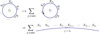
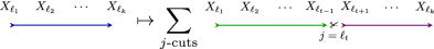
In the following, we sketch the action of the operator \(\partial ^{X_j}\) graphically. The convention is that the first letter of a word is the first after the cut (arrow tail) and the last letter corresponds to the one before the cut (arrow head).
-
One can represent the elements of \(\mathrm {im}\mathrm{Tr}_{N}\) as words on circles. For the NC-derivative \(\partial ^{X_j}: \mathrm {im}\mathrm{Tr}_{N}\rightarrow {\mathbb {C}}_{\langle n\rangle }\) one has
 (2.20)
where the ends of the line in the last figure are joined (multiplied).
-
In the next representation, each arrow belongs to a different tensor factor. Thus, \(\partial ^{X_j}: {\mathbb {C}}_{\langle n\rangle }\rightarrow {\mathbb {C}}_{\langle n\rangle }^{\,\otimes \, 2}\) acts as
Together, the two last pictures give the graphical interpretation of the proof of the proposition above.
-
Similarly, \(\partial ^{X_j}: {\mathbb {C}}_{\langle n\rangle }^{\,\otimes \, k} \rightarrow {\mathbb {C}}_{\langle n\rangle }^{\,\otimes \, k+1}\) j-cuts at all places of each tensor-factor (line):
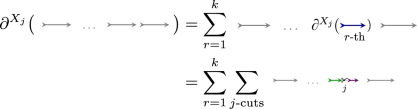 (2.21)


Example
The next examples shall be useful below:
-
On \({\mathbb {C}}_{\langle n\rangle , N}\) it holds \(\nabla ^2 \mathrm{Tr}(X_iX_j)= \sum _{k=1}^n2 e_i \delta _{i}^k \delta _{j}^k1_N\otimes 1_N = 2 e_i \delta _{j}^i 1_N\otimes 1_N \) from the last statement, since only the empty word is between the two letters.
-
On \({\mathbb {C}}_{\langle 1\rangle , N}={\mathbb {C}}\langle X\rangle \) with \(X^*=X\), \(\nabla ^2=( \partial ^X)^2\) and (\(m\ge 2\))
$$\begin{aligned} \nabla ^2 \mathrm{Tr}_{N}\Big (\frac{X^m}{m}\Big )=\sum _{\ell =0}^{m-2} X^\ell \otimes X^{m-2-\ell }. \end{aligned}$$(2.22)Now is evident that, even though \({\mathbb {C}}_{\langle 1\rangle , N}\) consists of ordinary polynomials, NC-derivatives are not ordinary.
Example
We compute a NC-Hessian and a NC-Laplacian on \({\mathbb {C}}_{\langle 2\rangle }= {\mathbb {C}}\langle A,B \rangle \). With aid of Claim 2.3 and setting \(g=\mathrm {diag}(e_1,e_2)= \mathrm {diag}(e_{{\mathsf {a}}},e_{{{\mathsf {b}}}})\):
which also explicitly shows the asymmetry of the Hessian. To compute, say, the entry (12) of this matrix, which corresponds to the operator \( \partial ^A \circ \partial ^B \), one has four matches: distributing the word ABAB on a circle as in 2.15, with the arrow tail at any letter B, the tip of the arrow can pair the A left (or clockwise) to it or the A to its right (counterclockwise). According to Claim 2.3 these contributions are, respectively, \(1\otimes BA\) and \(AB\otimes 1\) for each letter B in the word, hence the factor 2. The Laplacian is the trace of it,
2.2 The Algebraic Structure
We consider sums of monomials which either have the form \(X\otimes Y\) or \(X\otimes _\tau Y\) inside the same algebra:
where the second symbol emphasizes the matrix realization of the free algebra. On \({\mathcal {A}}_{n,N}\) there is a product \(\times \) defined in coordinates by
where \(\vartheta ,\varpi \) represent the twist \(\tau \) or its absence, and the sums are implicit. The twisted structure modifies the product according to:
Proposition 2.5
For monomials \(U,W,P, Q\in {\mathbb {C}}_{\langle n\rangle }\) one has
These rules can be remembered by identifying tensor product of monomials \(U\otimes W\) with the block diagonal element \(\mathrm {diag}(U,W)\in M_2({\mathbb {C}}_{\langle n\rangle })\) and each twisted product \(U\otimes _\tau W \) with the anti-diagonal \(\jmath \, \mathrm {diag}(U,W)=\big ({\begin{matrix} 0&{}W \\ U&{} 0 \end{matrix}}\big )\) for \(\jmath =\big ({\begin{matrix} 0&{}1 \\ 1&{} 0 \end{matrix}}\big )\). Then, the rules (2.5) are just ar restatement of matrix multiplication in \( M_2({\mathbb {C}}_{\langle n\rangle })\), but we do not state it a such since it does not work for polynomials. But in fact Eq. (2.5) can be proven in coordinates:
Proof
We prove the second rule: for \(a,\ldots , d=1,\ldots ,N\), one has
and that rule follows. The first rule (2.5) is obvious, the two left unproven are verified in similar way. \(\square \)
As a caveat, notice that
For monomials \(P,Q, U,W \in {\mathbb {C}}_{\langle n\rangle }\), we let also
where \(\varpi ,\vartheta \) stand for either \(\tau \) or an empty label.
Proposition 2.6
It follows that
Proof
We prove only the first one, the other proofs being similar:
\(\square \)
One can replace the new product by \(\times \), namely using
which holds due to
Notice that in Eq. (2.28) \(\tau \) no longer acts on the matrix indices and it has been transferred to the factors:
Since \(( PU \otimes _\tau WQ )_{ab;cd }=(PU \otimes WQ)_{cb;ad}\), another useful expression for the sequel is
Also, while the product \(\times \) loses the twist, \((1\otimes _\tau 1)^{\times 2} = (1 \otimes 1 )\), the \(\star \) product preserves it \((1\otimes _\tau 1)^{\star 2} = (1\otimes _\tau 1) \) and in fact \((1\otimes _\tau 1)\) is the unit element:
which follows from Proposition 2.6. Although it might be clear from the definition of \(\star \) that on \( {\mathbb {C}}_{\langle n\rangle }^{\otimes _\tau 2}\) it is associative—since there the first factor right multiplication and in the second ordinary matrix multiplication—it is reassuring to see that it is also associative if untwisted elements are implied:
Proposition 2.7
The product \(\star \) is associative on \({\mathcal {A}}_n\).
Proof
Let \(A,B,C,D,U,W,P,Q,T,S,X,Y \in {\mathbb {C}}_{\langle n\rangle }\). Using Proposition 2.6 one verifies straightforwardly that either bracketing,
or
yields due to the cyclicity of the trace the same result, namely:
\(\square \)
For the sequel, more important than the Hessian is its twisted version
Definition 2.8
The twisted NC-Hessian \(\mathrm{Hess}^\tau _\sigma \) is given by
In other words, by Proposition 2.5, \(\mathrm{Hess}^\tau _\sigma \) is obtained from \(\mathrm{Hess}_\sigma \) after exchanging the products \(\otimes _\tau \) and \( \otimes \).
Example
We exemplify computing the product of \(\mathrm{Hess}_\sigma ^\tau ( AABB) \), namely
with \(\mathrm{Hess}_\sigma ^\tau \big [\mathrm{Tr}A \mathrm{Tr}(A B B)\big ]\),
The diagonalFootnote 7 of \(\mathrm{Hess}_\sigma ^\tau [\mathrm{Tr}A \mathrm{Tr}(A B B) ] \star \mathrm{Hess}_\sigma ^\tau ( AABB)= \big ( {\begin{matrix} {\mathcal {P}} &{} * \\ * &{} {\mathcal {Q}} \end{matrix}}\big )\), which is computed entrywise with \(\star \), is given by (recall \(e_{{\mathsf {a}}}^2=e_{{{\mathsf {b}}}}^2=1\))
and
The \(M_n({\mathbb {C}})\)-trace (here for \(n=2\), \({\mathcal {P}} +\mathcal {Q}\)) of products of Hessians—or rather of their anti-commutator—will be shown to be fundamental for the RG-flow. The absolute (not only cyclic) order in the letters of the expressions for the twisted or untwisted Hessians of cyclic NC-polynomials absolutely matters. If one continues taking products of Hessians the order of the matrix factors does matter too (which is why one gets bulky expressions now). Only at the final stage, when we take traces, we can cyclically permute.
3 Random Noncommutative Geometries and Multimatrix Models
We briefly recall the foundations of fuzzy geometries, known to be rephrasable in terms of matrix algebras [66], in Barrett’s matrix geometry setting [8]. The original definition is given in terms of spectral triples, but in that definition the axioms implying the Dirac operator can be directly replaced by a characterization these boil down to.
3.1 Fuzzy Geometries as Spectral Triples
Given a signature \((p,q)\in {\mathbb {Z}}_{\ge 0 }^2\), a fuzzy (p, q)-geometry consists of a quintuple
whose elements we describe next. The inner product space V is given the structure of \(\mathcal {C}\ell (p,q)=\mathcal {C}\ell ({\mathbb {R}}^{(p,q)})\)-module. The action \({{\underline{\mathrm{c}}}}\) of the Clifford algebra on the basis elements \(\theta ^\mu \) of \({\mathbb {R}}^{(p,q)}=({\mathbb {R}}^{p+q},\mathrm {diag}(+_p,-_q))\), where the subindex in each sign means its repetition that many times, yields gamma-matrices \(\gamma ^\mu ={{\underline{\mathrm{c}}}}(\theta ^\mu )\). We assume that they satisfy,
that is, one has Hermitian or anti-Hermitian gamma-matrices according to whether \(\mu \) is a time-like (\(1\le \mu \le p\)) or a spatial index (\(p< \mu \le p+q\)). This in turn yields the chirality \(\gamma =(-\mathrm {i})^{s(s+1)/2} \gamma ^1\cdots \gamma ^{p+q}\), being \(s:=q-p\) the KO-dimension. The inner product of V together with the Hilbert–Schmidt inner product on \(M_N({\mathbb {C}})\) endow \({\mathcal {H}}= V\otimes M_N({\mathbb {C}})\) with the structure of Hilbert space the matrix algebra acts on in the natural way, ignoring V. Moreover, the KO-dimension determines three signs \(\epsilon , \epsilon ',\epsilon ''\in \{-1,+1\}\) via

The operator \(J= C\otimes (\)complex conjugation) on \({\mathcal {H}}\) defines the real structure. Here, \(C:V\rightarrow V\) is anti-unitary and satisfies \(C^2=\epsilon \) and \(C\gamma ^\mu =\epsilon '\gamma ^\mu C\) for each \(\mu =1,\ldots ,p+q\). Last, but most importantly, D, the Dirac operator, is a self-adjoint operator on \({\mathcal {H}}\) that satisfies the order-one condition \([[ D, Y' ], J Y J^{-1}]= 0\) for each \(Y,Y'\in M_N({\mathbb {C}})\). The signs in the table above imply, as part of the definition,
After the axioms are solved [8], for an even dimension \(q+ p\) (thus even KO-dimension), the Dirac operator has the form
where
-
\(\gamma ^\alpha =\gamma ^{\mu _{1}}\gamma ^{\mu _{2}}\cdots \gamma ^{\mu _{i_{2r-1}}}\) means the product of all indices included in an increasingly ordered multi-index \(\alpha =(\mu _{1}\cdots \mu _{i_{2r-1}})\). The hatted indices are those omitted from the list \(\{1,2,\ldots , p+q\}\). Notice that the sum runs only over multi-indices of odd cardinality; and
-
for any \(Y\in M_N({\mathbb {C}})\), \(k_\alpha \) are commutators or anti-commutators determined by \(\alpha \) via \(k_\alpha (Y)= X_\alpha Y + e_\alpha Y X_\alpha \), being \(X_\alpha \in M_N({\mathbb {C}})\) self-adjoint if \(e_\alpha =+1\) and traceless anti-Hermitian if \(e_\alpha =-1\).
For the first \(p+q\) values of i, \(e_i\) can be read off from \(\mathrm {diag}(e_1,\ldots ,e_{p+q})\), the signature; however, if \(p+q\ge 3\), the number n of matrices that parametrize D exceeds \(p+q\). This is also true for odd \(p+q\), for instance, in signature (0, 3) the Dirac operator can be written as

where \(L_i\in \mathfrak {su}(N)\) for each i and  are the quaternion units as a realization of the pertaining gamma-matrices. In odd dimensions, the chirality is trivial, which is why the anti-commutator term with a the Hermitian \(N\times N\) matrix H has a trivial coefficient, instead of a product of three different gammas matrices.
The complete criterion [61, Appendix A] that fully determines the signs in (2.1a) for even-dimensional fuzzy geometries implies multi-indices \(\alpha \), namely
After a signature (p, q) and the matrix size N are chosen, notice that the items \((M_N({\mathbb {C}}), V\otimes M_N({\mathbb {C}}), J, \gamma )\), called also a fermionic system, are fixed.
We let \({\mathcal {M}}_N ^{p,q}\) be the space of all the Dirac operators that complete the four objects into a fuzzy geometry. This spectral triple is finite-dimensional but does not fall into the classification made by Krajewski and Paschke–Sitarz [50, 64]. Using Eqs. (3.2) and (3.3) one can obtain \({\mathcal {M}}_N ^{p,q}\) in terms of \(\mathfrak {su}(N)\) and \({\mathbb {H}}_N\), the Hermitian matrices in \(M_N({\mathbb {C}})\). For instance \({{\mathcal {M}}_N^{0,4}} = {\mathbb {H}}_N^{\times 4} \times \mathfrak {su}(N)^{\times 4} \) for the Riemannian 4-geometry and \({\mathcal {M}}_N^{1,3} = {\mathbb {H}}_N^{\times 2} \times \mathfrak {su}(N)^{\times 6} \) for the Lorentzian case. However, the for formalism below it suffices to know the space of Dirac operators for two-dimensional fuzzy geometries:
When we work in fixed signature, we write \({\mathcal {M}}_N={\mathcal M_N^{p,q}}\), as above in Eq. (2.2).
3.2 The Spectral Action for Fuzzy Geometries
We review how to compute the Spectral Action \(\mathrm{Tr}f(D)\), in order to see its relation with chord diagrams, simultaneously setting the terminology for Sect. 7. We restrict the discussion below to two-dimensional geometry with otherwise arbitrary signature.
As remarked in [11], the computable spectral actions \(\mathrm{Tr}f(D)\) require f, which in the original Connes–Chamseddine formulation is a bump function around the origin, rather to be a polynomial, with \(f(x)\rightarrow +\infty \) as \(|x|\rightarrow \infty \). We thus restrict to positive, even powers of the Dirac operator, \(\mathrm{Tr}D^m\), which according to [61], can be computed from chord diagrams (C.D.) of m points. A chord diagram consists of a circumference with m marked points and m/2 arcs joining them. These diagrams encode traces of products of gamma matrices. For two-dimensional geometries, the description is relative simple, as no multi-indices are required:
where the value \( {\mathfrak {a}}(\chi )\) of the diagram \(\chi \) is defined by
Herein, for an m-point chord diagram and for each \(\mu _1,\ldots ,\mu _m=1,2\), one defines
where \(v\sim _\chi u\) means that the point u and v are joined by a chord of \(\chi \), and \(e_{\mu _v}\) are the signs in the signature \(\mathrm {diag}(e_1,e_2)\) of the fuzzy two-dimensional geometry. The rest of the elements is given by:
-
\({\mathscr {P}}_m\) is the power set of \(\{1,2,\ldots , m\}\)
-
for any \(\varUpsilon =\{i,j,\ldots ,k\} \in {\mathscr {P}}_m\), \(\mu (\varUpsilon )\) is the ordered set \((\mu _i,\mu _j,\ldots , \mu _k) \) and \(\mathrm {sgn}[\mu (\varUpsilon )]= \prod _{r\in \varUpsilon } e_{\mu _r} \), which is a sign
-
\(X_1=A\), \(X_2=B\) are the (random) matrices
-
the arrows on the product indicate the order in which it is performed; the right arrow preserves the order of the set one sums over and the left arrow inverts it.
A quick way to see that the Spectral Action is real, as it should be, bases on the observation that for each word w originated by a chord diagram \(\chi \), its adjoint \(w^*\) is originated by the mirror image of \(\chi \), denoted by \(\chi ^*\). But this being a chord diagram, it also appears summed in Eq. (3.4).

When the running indices in Eq. (3.5) take a particular value, we color the chords of the corresponding chord diagram: green, if at the ends of the chords there is a matrix A and violetFootnote 8 if it is B. To a fixed word, say \(B^4 A B^2 A^3\), generally many diagrams contribute,

and we now show that for certain words their sum cannot vanish. (This will lead to the well-definedness of the chosen truncation schemes in the FRGE.)
Lemma 3.1
Given any word \(w \in {\mathbb {C}}_{\langle 2\rangle }={\mathbb {C}}\langle A,B\rangle \) of even degree in each of its generators, \(\deg _A(w),\deg _B(w)\in 2 {\mathbb {Z}}_{\ge 0}\), it holds
That is, \(\mathrm{Tr}_{N}w\) has nonzero coefficient in the Spectral Action for a suitable power of the Dirac operator D.
Proof
We use a chord diagram argument. The general situation is that not only one chord diagram gives rise to w. Although the existence of such diagram having m chords is trivial to exhibit, there exists the risk that all those diagrams add up to zero. We now verify that this is impossible.
Suppose that \([\mathrm{Tr}_{N}w]\mathfrak a(\chi )\) does not vanish. This does not fix \(\chi \) but leaves still a freedom of exchanging all green chord ends, corresponding to A, among themselves and the same for and all violet ones, which correspond to B. (As a matter of illustration, for the word \(B^4 A B^2 A^3\) above the first line shows such moves among B-chords and the lower the A-chords.) All the diagrams \(\chi '\) with \([\mathrm{Tr}_{N}w]{\mathfrak {a}}(\chi ')\ne 0\) are obtained by either of these moves applied to the initial \(\chi \), hence the number of such \(\chi '\) is
which by assumption is the product of odd numbers, thus itself odd. Notice that the value of the diagrams \(\chi '\) might only differ from \(\chi \) by a sign, which is determined by the crossings of the chords. Indeed, in Eq. (3.5) the terms inside the curly bracket are fixed by hypothesis, and in (3.6) the product \( \prod _{\begin{array}{c} v,u=1;\, v\sim u \end{array} }^{m} \big ( e_{\mu _v}\delta ^{\mu _{v}\mu _{u}}\big )\) is the same. This implies that all the diagrams contributing to w never can cancel, as the sum \(\sum _{r=1}^{2 \ell -1} \varepsilon _r\) never does (for \(\ell \in {\mathbb {N}}, \varepsilon _r\in \{-1,+1\}\)). Therefore, the coefficient \([\mathrm{Tr}_{N}w](\mathrm{Tr}D^m )\) of \(\mathrm{Tr}_{N}w\) in \(\mathrm{Tr}D^m\) is by Eq. (3.4) nonzero. \(\square \)
Given an m-point C.D., a nontrivial partition is a set \(\varUpsilon \in {\mathscr {P}}_m\) which is neither empty, nor is complement is, \(\varUpsilon ^{\mathrm c}\ne \emptyset \). Such an \(\varUpsilon \) splits a diagram into product of traces of two words. These words can be read off from the diagram, according to (3.5) one counterclockwise the other clockwise. For instance,

produces \(\mathrm{Tr}_{N}(BAB^2A) \) from \(\varUpsilon ^{\mathrm c}\) (denoted by a shaded region) and \(\mathrm{Tr}_{N}(BAB^4A^3)\) from \(\varUpsilon \). These nontrivial subsets \(\varUpsilon \) play the main role in the next
Lemma 3.2
Let \({\mathbb {C}}_{\langle 2\rangle }={\mathbb {C}}\langle A,B\rangle \), as before. The coefficient of the double-trace \(\mathrm{Tr}_{N}(w_1) \mathrm{Tr}_{N}(w_2)\) in the Spectral Action is nontrivial for any word \(w=w_1\otimes w_2 \in {\mathbb {C}}_{\langle 2\rangle }\otimes {\mathbb {C}}_{\langle 2\rangle }\) satisfying \(\deg _A(w_1)+\deg _A(w_2),\deg _B(w_1)+\deg _B(w_2)\in 2 {\mathbb {Z}}_{\ge 0}\):
Proof
We use a similar, albeit longer, argument to the single-trace case of Lemma 3.1. Since otherwise the statement reduces to Lemma 3.1 above, we assume that neither \(w_1\) nor \(w_2\) is the trivial word \(1_N\). This means that only nontrivial partitions (\(\varUpsilon , \varUpsilon ^{\mathrm c}\ne \emptyset \)) can generate w, that is, if \({\mathfrak {a}} (\chi )\ne 0\), then w is listed in
with the condition that the first and the second traces yield simultaneously \(\mathrm{Tr}_{N}w_1\) and \(\mathrm{Tr}_{N}w_2\), in either correspondence. To wit, we have the following cases:
-
Case I. If \(\{ \mathrm{Tr}_{N}(w_1^*), \mathrm{Tr}_{N}(w_2^*)\}=\{\mathrm{Tr}_{N}(w_1), \mathrm{Tr}_{N}(w_2)\}\) as sets.
-
Case II. If the trace of both adjoint words are different, that is if \( \mathrm{Tr}_{N}(w_1^*) \ne \mathrm{Tr}_{N}(w_1), \mathrm{Tr}_{N}(w_2)\) as well as \(\mathrm{Tr}_{N}(w_2^*) \ne \mathrm{Tr}_{N}(w_1)\), \(\mathrm{Tr}_{N}(w_2). \)
-
Case III. For \(\{r,l\}=\{1,2\}\), if one coincides, \(\mathrm{Tr}_{N}(w_r^*) = \mathrm{Tr}_{N}(w_v)\), then the other does not, \(\mathrm{Tr}_{N}(w_{l}^*) \ne \mathrm{Tr}_{N}(w_u)\), \(\{u,v\}=\{1,2\}\).
In the first case, if \(\varUpsilon \in {\mathscr {P}}_m\) originates these words, so does \(\varUpsilon ^{\mathrm {c}}\), and their contribution to the previous sum is doubled, for \(\mathrm {sgn}[\mu (\varUpsilon )]=\mathrm {sgn}[\mu (\varUpsilon ^{\mathrm {c}})]\). Hence, in Case I, we can sum over half of the elements encompassed inside the curly brackets in (3.9). Since we excluded the trivial partitions, the total of sets in that sum is \(\#(\mathscr {P}_m)-2=2^m-2= 2\cdot (2^{m-1}-1)\). By hypothesis, the result of (3.9) is twice the sum over half elements, which is \(2^{m-1}-1\). But in Cases II and III, we also can do so, since \(\varUpsilon ^{\mathrm {c}} \) does not reproduce the word \(w_1\otimes w_2\), so we can ignore the half of the sets (3.9). In any case, the sum is a multiple of 2 (Case I) of, or directly (Cases II-III), a sum over \(2^{m-1}-1\) elements, which is an odd number, since \(w_1\otimes w_2\) is not the trivial word and thus \(m > 1\). Since the three cases are the only possibilities given the two words, the partial conclusion is that the set \(\varUpsilon \) in (3.9) runs over an odd number of independent elements.
Again, finding a C.D. \(\chi \) that generates w is not hard: one puts together the letters \(w_1w_2^*\) and joins by chords, matching letters. And again, this diagram is ambiguous up to a factor of \( (\deg _A(w_1w_2^*)-1)!! \times (\deg _B(w_1w_2^*)-1)!!\). Considering the initial paragraph, the total number of terms is
since the sum of all such diagrams is the product of (3.10) with the nonredundant odd number. By the same token as before, the sum over all the signs listed in Eq. (3.10) cannot vanish. \(\square \)
Concrete expressions for \(f(z)=\frac{1}{4}\big (\frac{z^2}{2} + \frac{z^4}{4}+\frac{z^6}{6}\big )\) are given below.Footnote 9 From now on, we agree to write down rather the operators \(\mathrm{Tr}^{\otimes \,2}\) should be applied to, in order to get the actual monomials in the action. As for the signs, it is convenient to set \(e_{{\mathsf {a}}}:=e_1\) and \(e_{{{\mathsf {b}}}}:=e_2\).
-
Quadratic operators:
$$\begin{aligned} 1_N \otimes \Big (\frac{e_{{\mathsf {a}}}}{2} A^2 +\frac{e_{{{\mathsf {b}}}}}{2} B^2 \Big ) + \frac{1}{2} (A \otimes A )+ \frac{1}{2} (B \otimes B ). \end{aligned}$$(3.11) -
Quartic operators:
$$\begin{aligned}&1_N \otimes \Big (\frac{1}{4} A^4+ \frac{1}{4} B^4 +e_{{\mathsf {a}}}e_{{{\mathsf {b}}}}A^2B^2 -\frac{1}{2} e_{{\mathsf {a}}}e_{{{\mathsf {b}}}}ABAB \Big ) \nonumber \\&\quad + AB \otimes AB +2e_{{\mathsf {a}}}e_{{{\mathsf {b}}}}A^2 \otimes B^2 + (e_{{\mathsf {a}}}A^3 + e_{{{\mathsf {b}}}}AB^2 ) \otimes A \nonumber \\&\quad +(e_{{\mathsf {a}}}A^2B + e_{{{\mathsf {b}}}}B^3 ) \otimes B +3 A^2\otimes A^2 + 3 B^2\otimes B^2 . \end{aligned}$$(3.12) -
Sextic operators: The part bearing a \(1_N\) factor is:
$$\begin{aligned}&1_N\otimes \big \{ e_{{\mathsf {a}}}A^6+ 6e_{{{\mathsf {b}}}}A^4 B^2-6 e_{{{\mathsf {b}}}}A^2(AB)^2+3e_{{{\mathsf {b}}}}(A^2B)^2 \nonumber \\&\quad + e_{{{\mathsf {b}}}}B^6+ 6e_{{\mathsf {a}}}A^2 B^4 - 6 e_{{\mathsf {a}}}B^2(BA)^2 + 3e_{{\mathsf {a}}}(B^2A)^2 \big \} , \end{aligned}$$(3.13a)and bi-trace terms are:
$$\begin{aligned}&A \otimes ( 2 A^5 +2 A B^4 +6 e_{{\mathsf {a}}}e_{{{\mathsf {b}}}}A^3B^2 -2 e_{{\mathsf {a}}}e_{{{\mathsf {b}}}}A^2BAB) \nonumber \\&\quad + B \otimes ( 2 B^5 +2 B A^4 +6 e_{{{\mathsf {b}}}}e_{{\mathsf {a}}}B^3A^2 -2 e_{{{\mathsf {b}}}}e_{{\mathsf {a}}}B^2ABA) \nonumber \\&\quad + 8 A B \otimes [ e_{{\mathsf {a}}}A^3B+ e_{{{\mathsf {b}}}}B ^3 A ] \nonumber \\&\quad + A^2 \otimes \big \{e_{{{\mathsf {b}}}}[8 A ^2 B ^2 -2 B A B A ] + e_{{\mathsf {a}}}[5 A ^4 + B ^4 ] \big \}\nonumber \\&\quad + B^2 \otimes \big \{e_{{\mathsf {a}}}[8 B ^2 A ^2 -2 A B A B ] + e_{{{\mathsf {b}}}}[5 B ^4 + A ^4 ] \big \}\nonumber \\&\quad + \frac{10}{3} (A^3 \otimes A^3 ) + 4 e_{{\mathsf {a}}}e_{{{\mathsf {b}}}}(A B^2 \otimes A^3) + 6 (A^2 B \otimes A^2 B) \nonumber \\&\quad + \frac{10}{3} (B^3 \otimes B^3 ) +4 e_{{{\mathsf {b}}}}e_{{\mathsf {a}}}(B A^2 \otimes B^3) +6 (B^2 A \otimes B^2 A) . \end{aligned}$$(3.13b)
Notice that neither
nor their cyclic permutations are allowed. The same holds for any nontrivial partition of these into two tensor factors (e.g., \(A\cdot A \otimes A\cdot A\cdot A\cdot B\)), as they are not compatible with chord diagrams, in the sense mentioned at the beginning of this subsection. We also remark that \(\otimes _\tau \)-products do not appear in the Spectral Action.
4 Deriving the Functional Renormalization Group Equation
We are interested in a nonperturbative approach and pursue the RG-flow governed by Wetterich–Morris equation (or FRGE). Polchinski equationFootnote 10 [62, Eq. 27] can be more suitable in a perturbative approach.
We start with the bare action \(S[\varPhi ]\) that describes the model at an “energy” scale \(\varLambda \in {\mathbb {N}}\) (ultraviolet cutoff). Let \(\varPhi \) be an n-tuple of matrices \(\varPhi = (\varphi _1,\ldots , \varphi _n) \in {\mathcal {M}}_{\varLambda }\), but the following discussion can be easily be made more general taking \(\varPhi \in M_N({\mathbb {C}})^{n}\). Motivated by fuzzy geometries, the bare action S is assumed to be a functional of the form
being P and each \(\varPsi _\alpha \) and \(\varUpsilon _\alpha \) in the finite sum a noncommutative polynomial in the n matrices, \(P, \varPsi _\alpha , \varUpsilon _\alpha \in {\mathbb {R}}_{\langle n \rangle }={\mathbb {R}}\langle \varphi _1,\ldots ,\varphi _n\rangle \). The trace \(\mathrm{Tr}=\mathrm{Tr}_ \varLambda \) is that of \(M_\varLambda ({\mathbb {C}})\).
Our derivation of Wetterich–Morris equation for multimatrix models is inspired by the ordinary QFT-derivation (e.g., [39]) for the first steps. Let
being \(J=(J^1,\ldots ,J^n) \in {\mathcal {M}}_N\) an n-tuple of matrix sources \(J^i\), and \(J\cdot \varPhi = \sum _{i=1}^n J^i \varphi _i \) the sum of the n matrix products. Here, \( \mathrm {d}\mu _\varLambda (\varPhi )\) is the product Lebesgue measure on \({\mathcal {M}}_\varLambda \), for which the notations \(\int _\varLambda [\mathrm {d}\varphi ] (\cdot )\) and \(\int _\varLambda {\mathcal {D}}\varphi (\cdot ) \) are also common, mostly in physics.
The fundamental object is the effective action \(\varGamma \), obtained by the Legendre transform of the free energy \(\mathcal {W}[J]\),
Here, X denotes the n-tuple \(X=(X_1,\ldots ,X_n)\) of classical fields \(X_i:=\partial ^{J^i} {\mathcal {W}}[J] = \langle \varphi _i\rangle \). The supremum creates the dependence \(J=J[X]\) and yields a functional depending only on X. Notice that since \(J\in {\mathcal {M}}_N\), each source obeys the same (anti)-Hermiticity relation \((J^i)^*=e_iJ^i\) as \(\varphi _i\), for each \(i=1,\ldots ,n\). As a consequence, \((J\cdot \varPhi )^*=(\varPhi \cdot J)\) and the classical fields obey the expected rules:
The effective action \(\varGamma [X]\) contains all the quantum fluctuations at all energy scales. In practice, one uses an interpolating average effective action that incorporates only the fluctuations that are stepwise integrated out; the average effective action \(\varGamma _N[X]\) results after integration of the modes having an energy larger than N (i.e. matrix indices larger than N), while lower degrees of freedom not yet integrated. The parameter N serves as a threshold splitting the modes in high and low; the latter sit in the \(N \times N\) block. Lowering N makes \(\varGamma _N[X]\) to approximate the full effective action \(\varGamma \).
The progressive elimination of degrees of freedom is obtained by adding a mass-like term
This regulator has been adapted from that of Eichhorn–Koslowski to the multimatrix case.Footnote 11 Typically the function \(R_N^\tau :\{1,\ldots ,\varLambda \}^4\rightarrow {\mathbb {R}}\) restricts the sum to some N-dependent region, but the sum limits in Eq. (4.4) allow for a freedom of regulators \(R_N^\tau \). Here, \(R_N^\tau \) is not meant as a matrix: in particular its k-th power \((R_N^\tau )^k\) does not imply \(k-1\) sums but rather the k-th power pointwise. This can be guaranteed by assuming
for a \({\mathbb {R}}\)-valued function \(r_N\), and to satisfy
which hold by imposing \(r_N(a,c)=r_N(c,a)\) for all a, c. Since \(\tau \) implies a twist in the product, we stress that \(R_N^\tau \) is not a multiple of the identity, only
is. The choice of \(R_N\) is arbitrary up to the following three conditionsFootnote 12:
-
1.
\((R_N)_{ab;cd} > 0\) for low modes, i.e. \(\max \{a,b,c,d\}/N\rightarrow 0\)
-
2.
\((R_N)_{ab;cd} \rightarrow 0\) for high modes, i.e. \(N/\min \{a,b,c,d\}\rightarrow 0\)
-
3.
\((R_N)_{ab;cd} \rightarrow \infty \) as \(N\rightarrow \varLambda \rightarrow \infty \)
which have the following effect, respectively:
-
1.
the infrared (IR) regulator suppresses low modes: as a result these are not integrated out, unlike high modes, which do contribute to the average effective action \(\varGamma _N\)
-
2.
is an initial condition for low N, i.e. ensures that one eventually recovers the full quantum effective action by lowering N
-
3.
is an initial condition for large N and ensures that one can recover the bare action S as \(N\rightarrow \varLambda \rightarrow \infty \) via the saddle-point approximation.

The idea behind the regulator \(R_N\) and its logarithmic derivative, here illustrated with a ‘bump function’: \(R_N\) protects the IR degrees of freedom, while those higher than N are integrated out. Thus, N is the “momentum threshold” that splits modes into high- and low-momenta
Thus, incorporating \(\Delta S_N\) to the action IR-regulates the functional
in terms of which one can obtain the interpolating average effective action
In practice, one uses the FRGE in order to determine it, instead of performing the path-integral. This equation is usually displayed in physics in terms of a supertrace \(\mathrm{STr}\) we next define on the superspace \(M_n({\mathbb {C}})\otimes {\mathcal {A}}_{n,\varLambda }=M_n({\mathcal {A}}_{n,\varLambda })\). Typical elements there form an \(n\times n\) matrix \({\mathcal {T}} \) with entries
for some matrices \({\mathcal {T}}^{(1)}_{ij}, {\mathcal {T}}^{(2)}_{ij} \in {\mathbb {C}}_{\langle n \rangle ,\varLambda }\), whose four remaining entries we separate using a vertical bar, to avoid confusion:
We let also \({\mathbf {1}}= 1_n\otimes 1_\varLambda \otimes 1_\varLambda \), lest our notation becomes very loaded (which is a neutral element if \({\mathcal {A}}_n\) is endowed with \(\times \)) but also notice that according to Eq. (2.30) only \({\mathbf {1}}_\tau = 1_n\otimes 1_\varLambda \otimes _\tau 1_\varLambda \) acts as a unit with respect to the \(\star \)-product. The supertrace is given by
Since knowing the matrix size will be useful, we use \(\mathrm{Tr}_{\varLambda }^{\otimes 2}\) sometimes instead of \(\mathrm{Tr}_{{\mathcal {A}}_2}\), but as the next \(n=2\) example shows, it is important to be careful with twisted products whose factors are merged inside a same trace:
Proposition 4.1
The interpolating effective action \(\varGamma _N\) of a matrix model with \(X=(X_1,\ldots , X_n)\in {\mathcal {M}}_N^{p,q}\) satisfies for each \(N\le \varLambda \) Wetterich–Morris equation, which reads

being \(t=\log N\) the RG-flow parameter and \(\sigma =\mathrm {diag}(e_1,\ldots ,e_n)\) with \( X^*_{i}=\pm X_i\,\) iff \(e_i=\pm 1\). These signs are determined by the signature (p, q) of the fuzzy geometry that originates the matrix model—which for dimensions \(p+q \le 2\) coincides with \(g=\mathrm {diag}(e_1,\ldots , e_{p+q})\)—and else are given by Eq. (3.3). The quotient of operators is meant with respect to the \(\times \) product.
Also \(n=2\) if \(p+q=2\) and \(n=8\) if \(p+q=4\), with general rule \(n=2^{p+q-1}\) as far as \(p+q\) is even [61] and \(R_N\) is economic notation for \(1_n\otimes R_N \). After the proof, we provide the strategy to compute the RHS. The quantity in the “denominator” of the FRGE requires some care; its well-definedness is addressed in Sect. 5.2.
Proof
Directly from the definition of the interpolating action one has
Recalling that \(X_i= {\mathcal {Z}}_N^{-1}\partial ^{J^i}{\mathcal {Z}}_N \), one can use
in order to re-express \(\partial _t(\Delta S_N)\) appearing in the integrand in the first term, \({\mathcal {Z}}_N[J]^{-1}\int (-\partial _t \Delta S_N) \mathrm {e}^{-S-\Delta S_N+\mathrm{Tr}(J \cdot \varphi )} \mathrm {d}\mu _\varLambda (\varPhi ) \), of Eq. (4.10) to obtain
The rest relies on the use of the superspace chain rule
Passing from the first to the second line is implied by taking the derivative with respect to \(X_j\) of the IR-regulated quantum equation of motion, that is of
In the second line \(\partial ^{X_k}_{ab} J\) is a matrix (for fixed a, b) and the trace \(\mathrm{Tr}( X \cdot \partial ^{X_k}_{ab} J )\), which equals \(\partial ^{X_k}_{ab} {\mathcal {W}}_N[J]\) by the chain rule, is taken with respect to those tacit indices of J. In the other trace-term, the shown indices a, b are excluded, so traces are taken for the remaining ones (the dots in \(R_N^\tau \)); the symmetries (4.5) of \(R_N^\tau \) have been used too. Hence, indeed
after Eq. (4.6) and the index symmetries implied by it. Denoting by \(\cdot _n\) the product in the \(M_n({\mathbb {C}})\) tensor factor (of the superspace), one can moreover replace \((\mathrm{Hess}^J \mathcal W_N)_{ki}= \partial ^{J^k} \partial ^{J^i} {\mathcal {W}}_N[J]\) by the inverseFootnote 13 of
after using \(\sigma =\mathrm {diag}(e_1,\ldots ,e_n)\) and the fact that \(1/e_i =e_i\) (since \(e_i=\pm \)). One has
The result follows from Eq. (4.11), after realizing that the LHS of (4.12) is \( \delta _{ij}\delta _{ux} \delta _{vy}=(1_n\otimes 1 \otimes _\tau 1 )_{ij|yx;uv}=(\mathbf{1}_\tau )_{ij|yx;uv}\). In order to invertFootnote 14 the Hessian of \({\mathcal {W}}\), we use
where the \(\star \) product and the twisted Hessian can now be recognized. Therefore,
We renamed indices and we used the symmetry \((R_N^\tau )_{ab;cd} = (R_N^\tau )_{ba;cd}\). \(\square \)
The RHS of the FRGE is usually interpreted in terms of a ribbon loop  , the thick ribbon being the full propagator. For the present FRGE this picture is obtained by interpreting the ribbon as the supertrace \(\mathrm{Tr}_n\otimes \mathrm{Tr}_{\varLambda }^{\otimes 2}\),

The source marked with a crossed circle is the RG-time derivative term. In order to stress the meaning of the last equation, we consider an ordinary Hermitian n-matrix model. Proposition 4.1 then restricts to signature (n, 0), so each \(e_i=1\), \(i=1,\ldots ,n\).
Corollary 4.2
(FRGE for Hermitian multimatrix models). Wetterich–Morris equation for Hermitian n-matrix models is given by
Proof
It is immediate from Proposition 4.1, since for Hermitian matrices one has \(\sigma =1_n\). \(\square \)
5 Techniques to Compute the Renormalization Group Flow
The next sections explain how to compute the RHS of the FRGE.
5.1 Projection and Truncations
The RG-flow generates the infinitely many operators that the symmetries allow. Feasibility forces us first to project each matrix \(X_i\) to a \(N\times N\) matrix \(X_i^{(N)}\) and then truncate \(\varGamma _N[X^{(N)}]\) to Ansätze implying finitely many operators \(\mathcal {O}_I\) indexed by words I of the free algebra. Since this projection will be assumed for the rest of this paper, for the sake of lightness we agree to write \(X^{(N)}\) as X. Some truncation schemes are:
-
Single trace truncation:
$$\begin{aligned} \varGamma _N[X]= N \sum _I \bar{{\mathsf {g}}}_I(N)\mathrm{Tr}_{N}({\mathcal {O}}_I(X)). \end{aligned}$$ -
Bi-tracial truncation:
$$\begin{aligned} \varGamma _N[X]&= N \sum _I\bar{{\mathsf {g}}}_I(N)\mathrm{Tr}_{N}({\mathcal {O}}_I(X)) \end{aligned}$$(5.1)$$\begin{aligned}&\quad + \sum _{I,I'} \bar{{\mathsf {g}}}_{I|I'}(N)(\mathrm{Tr}_{N}\otimes \mathrm{Tr}_{N})(\overbrace{{\mathcal {O}}_I(X)\otimes {\mathcal {O}}_{I'}(X)}^{\mathcal O_{I|I'}(X)}). \end{aligned}$$(5.2) -
Degree-k truncation:
$$\begin{aligned} \varGamma _N[X]= \sum _{\begin{array}{c} I_1,\ldots , I_{\alpha } \\ \sum _\nu \mathrm {deg } {\mathcal {O}}_{I_\nu }(X)\le k \end{array} } \frac{(\bar{{\mathsf {g}}}_{I_1|I_2|\ldots | I_\alpha })(N)}{N^{k-1}} \mathrm{Tr}_{N}^{\otimes j} \bigg ( \bigotimes _{\nu =1}^\alpha {\mathcal {O}}_{ I_\nu } (X) \bigg ), \end{aligned}$$
where \(\bar{{\mathsf {g}}}_{\ldots }(N)\) are the coupling constant, to be later renormalized to \({{\mathsf {g}}}_{\ldots }(N)\), the physical value.
We warn that this choice will be taken together with the assumption of N being large. The price to be paid is the un ability to recover the full effective action (which otherwise would be obtained by \(\lim _{N\rightarrow 1} \varGamma _N \)) not only because N is large, but also because we compute in a projection.
5.2 The \(FP^{-1}\) Expansion in the Large-N Limit
Based on the procedure introduced in [32] for Hermitian matrix models—which soon will be modified—we split the full propagator, for us \( \mathrm{Hess}_\sigma \varGamma _N[X] + R_N =P \oplus F[X]\), into field-dependent and field-independent parts. In our multimatrix case, with signs \(\sigma =\mathrm {diag}(e_1,\ldots , e_n)\) given by Eq. (2.1a), we get \( F[X]:=\mathrm{Hess}_\sigma \varGamma _N [X] -(\mathrm{Hess}_\sigma \varGamma _N\big |_{X=0}) \) and \(P:= R_N +(\mathrm{Hess}_\sigma \varGamma _N\big |_{X=0})\). We now simplify the treatment assuming that
for the rest of the paper. This is not the most general case and particularly excludes for the time being mixed signatures left for later study; however, this simplification has the advantage of leading to a P that is the identity matrix multiplied by a function \( \{1,\ldots ,\varLambda \}^4\rightarrow {\mathbb {C}}\) denoted by the same letter, \(P= (e^2 Z+R_N ) {\mathbf {1}}=(Z+R_N ) {\mathbf {1}}\) since \(e^2=1\). Notice that both Z and \(R_N\) being always positive P is invertible. In particular, powers \(P^\ell \) of P are meant pointwise (not as a matrix or tensor). One therefore has the commutation of P with the field part F[X],
It is important to realize in which sense the regulated Hessian of the interpolating action is an inverse of the Hessian of \(\mathcal W_N\) in source space, as this defines the way we have to take the Neumann series to invert \(\mathrm{Hess}_\sigma ^\tau \varGamma + R_N^\tau \). Although in the \(M_n({\mathbb {C}})\) factor of superspace this is an ordinary matrix product—see the groupoid property in the indices i, j, k inside the proof of the FRGE, \(\{\mathrm{Hess}_\sigma \varGamma _N [X] + R_N \}_{ij\mid xb;ay} (\mathrm{Hess}^J_{\sigma }{\mathcal {W}}[J])_{jk\mid cx;yd } =(1_n \otimes 1 \otimes _\tau 1 )_{ik \mid ab;cd}\)—each entry of that matrix is multiplied according the product \(\star \); this product is easier to recognize in Eq. (2.29). That is to say, the way to invert in FRGE the regulated Hessian as dictated by the proof of the FRGE, is the algebra \(M_n({\mathcal {A}}_n,\star )\) and not \(M_n({\mathcal {A}}_n,\times )\). The commutation Eq. (5.3) can be replaced by
since for \(({\mathcal {A}}_{n},\star ) \) the unit is \(1\otimes _\tau 1\) and \(P_\tau \) can be treated as a scalar function. We take the Neumann series of the twisted version \((\mathrm{Hess}_\sigma ^\tau \varGamma _N[X]+R_N^\tau )^{-1}\). Namely by Eq. (5.3b),
Underlying this structure is the independence of P from the matrices \(X=\{X_j\}\). Thus, when evaluated, \((P_{\tau })^\ell \) sits in the constant part of \({\mathcal {A}}_{n,\varLambda }\), so powers of \(P_\tau \) act on the field part by scalar multiplication. On the other hand, \((F_\tau [X]) ^{\star k}\) does mean the matrix product in the field part (2.5) of \({\mathcal {A}}_{n,\varLambda }\). Then, using the associativity of \(\star \) (Proposition 2.7), it is routine to check that the series (5.4) serves as inverse of \(P_\tau \oplus F_\tau [X]\) in the sense that their product in either order yields \({\mathbf {1}}_\tau =1_n\otimes 1_\varLambda \otimes _\tau 1_\varLambda \). Therefore,
Assuming a truncation necessitates a compatible supertrace, \(\mathrm{STr}_{N}\). Since functions \(G:\{1,\ldots ,\varLambda \}^4 \rightarrow {\mathbb {C}}\) act multiplicatively on the fields, we let
for W a field (\(\deg W\ne 0\)) in \(M_n({\mathbb {C}})\otimes {\mathcal {A}}_{n,\varLambda }\). Here, \(W_N\) is the same matrix of words W projected to \(M_n({\mathbb {C}})\otimes {\mathcal {A}}_{n,N}\). Also, \(\mathrm{STr}\) is defined to be identically zero on the ‘constants’ of the free algebra (in the terminology of Sect. 2), or
This follows from any of the previous Ansätze for \(\varGamma _N\), but it holds in general on physical grounds, since that constant part in the action corresponds to the vacuum energy [55]. However, the constant part of the algebra cannot be fully ignored since is the one that regulates the RG-flow and that part appears multiplying the fields.
Remark 5.1
It would be interesting to answer whether the vanishing of \(\mathrm{STr}_{N}(L)\) (here and in the physics literature, as part of the definition) yields constraints on the IR-regulator. Namely, to explore the conditions that the equation \(\mathrm{STr}_{N}(P^{-1}1_N\otimes 1_N)=0\) imposes on \(R_N\), if one does not automatically include in the definition the condition (5.7).
Proposition 5.2
The RG-flow is generated by the noncommutative Laplacian scaled by \(\varrho := \sum _{a,b,c,d} (\partial _t R_N \cdot P^{-2})_{ab;cd}\). That is, in the ‘tadpole approximation’, the FRGE is given by
Proof
The tadpole approximation means to cut Eq. (5.5) to \(k=1\). It is immediate that one can undo the twists from the Hessian and \(R_N^\tau \) altogether, with that of \(\partial _t R_N^\tau \) since in this simple case \(\star \) is not implied. By Eq. (5.6) this means that
were Eq. (5.7) has been used from the first to the second line, and from there to the third too. Now, \( F[X] + F[0] = \mathrm{Hess}_\sigma \varGamma _N[X] \), which traced over the first \(M_n({\mathbb {C}})\) factor, is by definition the NC-Laplacian. \(\square \)
We next justify the approximation given in Eqs. (5.6)–(5.7) and relate it with the definition of \(\mathrm{STr}\). Notice that the support of the function \(G^{(N)}_k:\{1,\ldots ,\varLambda \} ^ 4 \rightarrow {\mathbb {R}}\) given by \(G^{(N)}_k=(\partial _t R_N) \cdot P^{-(k+1)}\) becomes an N-dependent region of \(\{1,\ldots ,\varLambda \} ^ 4\). Generally, one cannot find a function \(f_n(N)\) such that \(\mathrm{STr}(G_k^{(N)}\cdot W[X])=f_k(N) \cdot \mathrm{Tr}_n\otimes \mathrm{Tr}_{{\mathcal {A}}_{n,N}}(W_N[X])\), or explicitly such that
holds for a \(W[X] \in M_n({\mathcal {A}}_{n,\varLambda }) \) in the field part of the free algebra, with \(W_N[X] \in M_n({\mathcal {A}}_{n,N})\). What is done in practice is to assume this replacement, but in return to let the function \(f_k(N)\) be governed by the FRGE. We moreover use a regulator \(R_N\) whose support is inside \(\{1,\ldots ,N\} ^ 4\).
In order to exploit the FRGE, one needs to compute the first powers of the expansion (5.4). Defining \(\tilde{h}_k(N)=\sum _{a,b,c,d}^\varLambda (G^{(N)}_k)_{ab;cd}\), which, since neither \(\partial _t R_N\) nor \(P^{-(k+1)}\) have field dependence, equals
one obtains after projecting
where \(\mathrm{Tr}_{N}\otimes _\tau \mathrm{Tr}_{N}({\mathcal {Q}})= \mathrm{Tr}_{{\mathcal {A}}_n}((1_N\otimes _\tau 1_N) \times {\mathcal {Q}})\) in terms of which we \(\mathrm{STr}_{N}^\tau \). That twist comes from \(R_N^\tau \), whose untwisted part was absorbed in the functions \(G^{(N)}_k\). We remark that Eq. (5.6) does not take into account the symmetry breaking caused by the regulator \(R_N\), which is related to ignoring the modified Ward–TakahashiFootnote 15 identity [54] caused by \(R_N\).

6 “Coordinate-Free” Matrix Models
We cross-check that, notwithstanding the somewhat different statements, our purely algebraic approach yields, for the Hermitian case with \(n=1\), the results that [32] presented in “coordinates” (that is, written with matrix entries). Here, we also calibrate the IR-regulator for later use in Sect. 7.
The interpolating action \(\varGamma _N[X]\) is given by (applying \(\mathrm{Tr}_{N}^{\otimes 2}\) to) the next operators that define our truncation: [1]
Since \(n=1\), the NC-Laplacian equals the NC-Hessian \(\partial ^2\), which on \(\mathrm{Tr}{\mathcal {O}}\) for an operator \({\mathcal {O}}\in {\mathbb {C}}_{\langle 1\rangle } \) equals \((\partial \circ {\mathscr {D}}) {\mathcal {O}}(X)\) by Claim 2.1. So, by Claim 2.3 and Eq. (2.17) one gets
One now “twists” these equations. The expression for \(F[X]=\mathrm{Hess}^\tau \varGamma [X] - Z (1_N\otimes _\tau 1_N )\) follows from the first equation in this list (after exchange of the tensor product with the twisted version). We keep odd-degree operators in F, even if we first included even-degree ones, since we need powers of F and even-degree operators are generated from odd-degree ones.
By neglecting odd-degree after taking the \(\star \)-powers of F[X], as well as truncating them to degree-six operators, the \(FP^{-1}\) expansion (5.10) in this setting reads:
up to the third nontrivial term (\(h_r=0\) for \(r\ge 4\)) in the \(FP^{-1}\)-expansion. This equation was obtained using the product rules of Proposition 2.5: For instance, the cubic term in \(\bar{{\mathsf {g}}}_4\) in the fifth line of (6.1) comes from \(P^{-4}F^{\star 3}\), more concretely from
where the dots omit other terms in the cube of F. Graphically, the \(\bar{{\mathsf {g}}}_4^3\)-contribution to \(\bar{{\mathsf {g}}}_6\) is (cf. Eq. (4.16) too)

We let \(h_k=\lim _{N\rightarrow \infty }Z^k{{\tilde{h}}}_k(N)/N^2 \), which due to Eq. (5.9) is independent of Z, and choose later an explicit regulator \(R_N\) that makes \(h_k\) only dependent on k in the large-N limit. Thereafter, the contributions to the \(\beta \)-functions coming from quantum fluctuationsFootnote 16 can be read off from Eq. (6.1). To state the quantum fluctuations in terms of the renormalized quantities (without bar), one needs to find the way these scale with Z and N. We let \(\bar{{\mathsf {g}}}_{2k}=Z^{a_k} N^{-b_k} {\mathsf {g}}_{2k}\) and \(\bar{{\mathsf {g}}}_{u|2k-u}=Z^{j_k} N^{-i_k} {\mathsf {g}}_{u|2k-u}\) (for even u, with \(0<u<2k \)).
To solve for \(a_k,b_k,i_k,j_k\), one asks the equation \(\beta _{I} = \partial _t {\mathsf {g}}_{I} \) to remain finite for each operator \({\mathcal {O}}_I\) as \(N\rightarrow \infty \). This leads to
These scalings, together with the quantum fluctuations from Eq. (6.1), yield for the anomalous dimension \(\eta =-\partial _t \log Z\) and the \(\beta \)-functions in the large-N limit:
We only are in debt with the explicit regulator \((R_N^\tau )_{ab;cd}=r_N(a,c)\delta _{a}^d\delta _{c}^b\) for \(r_N\) defined on \(\{1,\ldots , \varLambda \}^2\) and given by
being \(\varTheta _{{\mathbb {D}}_N}(a,b)\) the indicator function in the disc \(a^{2}+b^{2}\le N^{2}\).

The plot shows the support of the chosen IR-regulator \(r_N(a,b)\), contained in the square \({\mathbb {R}}^+_{\le N} \times {\mathbb {R}}^+_{\le N} \). (The white quarter of disk means a truncation of the graph around the origin.)
It turns out that for this regulator, \(Z^k{{\tilde{h}}}_k/N^2\) indeed converges to a number \(h_k\) independent of N, when this parameter is large. The first values are in fact
Inserting the four fixed point equations, i.e.  for \(I=2,4,2|2 \) and 2|4, one finds, on top of the Gaussian trivial fixed point (\({\mathsf {g}}_I=0\) for each I), several fixed points, tagged here with a little black diamond. The interesting one to be reproduced is expected be \(-1/12\), the critical value of \({\mathsf {g}}_4\) for gravity coupled to conformal matter [25]. The latter has been identified in [32], who report
  using the very same truncation.Footnote 17 In contrast, we get

This fixed point, obtained with the IR-regulator \(r_N\) of Eq. (6.4) gets far closer ( ) to the exact value \({\mathsf {g}}_{\mathrm {c}}=-1/12=-0.083\bar{3} \), which suggests that we should stick to our \(r_N\) for the two-matrix models treated next.
7 Two-Matrix Models from Noncommutative Geometries
7.1 Theory Space
The conventions for the coupling constants are the following, with numerical factors incorporated later. For
we associate with each operator the following coupling constants:
Notice the alternating convention in the letters. For coupling constants of type \({{\mathsf {c}}}\) and \({{\mathsf {d}}}\) (mnemonics: ‘combined’ and ‘disconnected’) some care is needed. Operators can always begin with the highest power of A, which for \({{\mathsf {c}}}\) is never zero—otherwise the respective operator is a pure power of either A or of B—in order to reduce the number of constants. This is due to the possibility to cyclicly reorder (\(\sim \)) the words, as these appear inside a trace. Only the first and last parameters can be zero for \({{\mathsf {d}}}\)-constants. In order to include an odd number of powers of the letters, the last integer is allowed to be zero. If this is so, we agree to omit the rightmost zero.
Both conventions are illustrated with \(ABA\otimes BAB \sim ABAB^0\otimes AB^2 \), whose coupling constant is \({{\mathsf {d}}}_{1110|12}={{\mathsf {d}}}_{111|12}\). On the other hand a leftmost zero is important: from the definition \({{\mathsf {d}}}_{l_1l_2\cdots l_t|I } \ne {{\mathsf {d}}}_{0l_1 l_2\cdots l_t| I}\), since \(A^{l_1}B^{l_2} \cdots B^{l_{2t}} \ne A^{0} B^{l_1} A^{l_2} \cdots A^{l_{2t}} \). Notice that \({{\mathsf {d}}}\) has to satisfy a symmetry condition: \({{\mathsf {d}}}_{I|I'}={{\mathsf {d}}}_{I'|I}\) for any integer multi-indices \(I,I'\) (since the respective operators do), so we only keep one of the two.
As before, a bar on a coupling constant, \({\bar{{{\mathsf {a}}}}},\ldots ,{\bar{{{\mathsf {d}}}}}\), denotes its unrenormalized value, whose N-dependence we do not show, for the sake of keeping the notation compact.
7.2 Compatibility of the RG-Flow with the Spectral Action
We now prove that in the double-trace truncation the RG-flow does not generate more operators than those allowed by the NCG-structure.
Proposition 7.1
Pick a two-matrix model that includes finitely many single-trace operators \(\mathrm{Tr}_{N}Q\), \( Q\in {\mathbb {C}}_{\langle n\rangle , N}\), and assume that each of them appears (probably with other coefficient) in the Spectral Action for certain fuzzy two-dimensional geometry. Then, the RG-flow generates at any order in the \(FP^{-1}\)-expansion exclusively operators that appear again, generally with a different nonzero coefficient, in the Spectral Action \(\mathrm{Tr}f(D)\), which in the worst case would require a suitable (generally higher-degree) polynomial f.
Proof
Suppose that \(\mathrm{Tr}_{N}Q\), with \(Q\in {\mathbb {C}}_{\langle n\rangle , N}\), features in the Spectral Action for a fuzzy geometry. First, we show that the NC-polynomial \((\partial ^A \circ \partial ^A \mathrm{Tr}_{N}Q )^{\star k} \in {\mathcal {A}}_2\) appears for each \(k\in {\mathbb {Z}}_{\ge 1 }\) in the Spectral Action for the same fuzzy geometry—we argue later for the most general case containing mixed derivatives. From (2.16), \(\partial ^A \circ \partial ^A \mathrm{Tr}_{N}Q \) contains two powers of A less than the original NC-polynomial Q, which, since it appears in the Spectral Action, has an even degree \(\deg _A(Q),\deg _B(Q) \in 2 {\mathbb {Z}}_{\ge 0}\). Therefore, so does the double derivative, and by Lemmas 3.1 and 3.2, \(\partial ^A \circ \partial ^A \mathrm{Tr}_{N}Q \) appears in the Spectral Action. The condition holds for any power \((\partial ^A \circ \partial ^A \mathrm{Tr}_{N}Q )^{\star k}\) since the even-degree conditions are still satisfied and therefore each monomial \(w_1\otimes w_2\) or \(w_1\otimes _\tau w_2\) in \((\partial ^A \circ \partial ^A \mathrm{Tr}_{N}Q )^{\star k}\) appears in the Spectral Action \(\mathrm{Tr}f(D)\) for a polynomial f with nonzero coefficient in degree m, being \(m=m(w_1,w_2)\) given by Lemma 3.2.
The argument is still true for different NC-polynomials \(Q_i\) appearing in the original Spectral Action and the even-degree argument holds not only for powers of double derivatives of these, but can be clearly extended to
since in the product the same derivative \(\partial ^{X_k}\) (\(X_k \in \{A,B\}\)) appears an even number of times. All the NC-polynomials generated by the supertrace in the FRGE are of this form, and having even degree in both matrices, the argument above leads in this case to the result. \(\square \)
Proposition 7.1 says that if the bare action would contain only single-trace operators, then all the operators that the RG-flow generates, including double-trace operators, are compatible with the structure of fuzzy geometries. This implies that for a realistic bare action, which includes only double-trace operators as dictated by the Spectral Action for a fuzzy two-dimensional geometry, the RG-flow generates (up to triple traces excluded in the truncation) exclusively NCG-compatible operators. Both structures can therefore be seen as highly compatible.
7.3 The Truncated Effective Action
The model we adopt includes all the operators appearing in the Spectral Action for fuzzy geometries computed in [61] up to the sixth degree. For two-dimensional fuzzy geometries,
where \( P, \varPsi _\alpha ,\varUpsilon _\alpha \in {\mathbb {C}}_{\langle 2\rangle } ={\mathbb {C}}\langle A,B\rangle \) are given, degree by degree by Tables 1 and 2. There, a dot means the usual matrix product. The number of running coupling constants turns out to depend not only on the dimension, but also on the signature of the fuzzy geometry, see Table 3. We stress that for the quartic and quadratic operators we do take the coupling constants with the symmetry factors and signs present in the NCG-action. For the sextic operators we drop the numerical normalization factors, in order to avoid rational coefficients.
7.4 The \(\beta \)-Functions
We present now the set of equations satisfied by the fixed points  , determined by the vanishing of all \(\beta \)-functions \(\beta _{\!\cdot \!\!\!}=\partial _t {\mathsf {g}}_{\!\cdot \!\!}\). We recall that
which are real numbers in the case of the quadratic regulator of Sect. 6 and whose values are given by Eq. (6.5). The next result is more transparent if one does not specify these coefficients yet (and holds for any \(R_N\) verifying that these \(h_k\) are all independent of N).
Theorem 7.2
Assuming \(Z_{{{\mathsf {a}}}}=Z_{{{\mathsf {b}}}}=:Z\), to the second order in the \(FP^{-1}\) expansion \((h_r=0, r\ge 3)\), in the double-trace and sixth-degree truncation, the \(\beta \)-functions of the two-matrix model corresponding to a two-dimensional fuzzy geometry with signature \(\mathrm {diag}(e_{{\mathsf {a}}},e_{{{\mathsf {b}}}})\) are given in the large-N limit by the following blocks of equations:
First, the degree-2 operators yield the anomalous dimension and following relations:
The next block encompasses the connected quartic couplings:
The \(\beta \)-functions for the connected sextic couplings are
And a last block of \(\beta \)-functions for the disconnected couplings is located in Section III of Supplementary Material.
Proof
We address first the first order in the \(FP^{-1}\)-expansion. This part of the proof consists of the following steps:
-
Step 1. The computation of the second-order derivatives of all the operators, determine the NC-Hessians to insert in the \(FP^{-1}\)-expansion. We now give the NC-Hessians computed using Claim 2.3 as well as their trace, the NC-Laplacian using Eq. (2.17). We write some of them down up in Table 4 to quartic operators; those omitted might be obtained by the exchange \(A\leftrightarrow B, e_{{\mathsf {a}}}\leftrightarrow e_{{{\mathsf {b}}}}\) (and adjusting the matrix structure). The expressions for \(\mathrm{Hess}_\sigma \mathrm{Tr}(A A B B)\) and \( \mathrm{Hess}_\sigma \{\mathrm{Tr}(A) \mathrm{Tr}(A B B)\}\), the quartic operators missing in Table 4 were already given in Example 2.2 and show that the complexity rapidly grows. For the sake of readability, the bulkier sixth-degree operators completing the running 34 or 48 involved in the flow, are located in Section II of Supplementary Material.
-
Step 2. To the first order, one computes the regularized NC-Laplacian \(F = e_{{\mathsf {a}}}F_{{\mathsf {aa}}}+ e_{{{\mathsf {b}}}}F_{{\mathsf {bb}}}\) of the effective action in terms of
$$\begin{aligned} F_{{\mathsf {aa}}}=(\partial ^A \circ \partial ^A) \varGamma _N [A,B]-(\partial ^A \circ \partial ^A) \varGamma _N [A,B]\big |_{A=B=0} \end{aligned}$$and of
$$\begin{aligned} F_{{\mathsf {bb}}}=(\partial ^B \circ \partial ^B) \varGamma _N [A,B]-(\partial ^B \circ \partial ^B) \varGamma _N [A,B]\big |_{A=B=0}. \end{aligned}$$ -
Step 3. One takes the double traces of the resulting expression. The \(h_1\)-terms, i.e. the trace \(\mathrm{Tr}_{N}^{\otimes 2}\) of the NC-Laplacian, read as in Section IV of the Supplementary Material. From that expression one can deduce some of the quantum fluctuations. In the large-N limit, according to the scalings given in Tables 1 and 2, the matching of the \(h_1\) coefficients in the fixed point equations given in the statement can be verified. The scaling \(N^{-m(Q)}\) of the coupling constant \({\mathsf {g}}_{Q}\) that corresponds with the operator \(Q\in {\mathbb {C}}_{\langle 2\rangle }\otimes {\mathbb {C}}_{\langle 2\rangle }\) determines the coefficient of the form
$$\begin{aligned} \left( \frac{\deg _A (Q)+\deg _B(Q)}{2}\eta + m(Q)\right) \times {\mathsf {g}}_{Q}, \end{aligned}$$appearing in the \(\beta _Q\)-function.
We now sketch the second order: Having computed in Step 1 the 48 NC-Hessians, one \(\star \)-squares the \((48-2)\) Hessians appearing in F (the two subtracted operators are \(A^2\) and \(B^2\) whose Hessian is absorbed in P). The \(\sim \,10^3\) matrices of size \(2\times 2\) with NC-polynomial entries are omitted, but each of these was computed as in Example 2.2. Then, one traces \(F^{\star 2}\) in superspace to collect quantum fluctuations for each operator. Taking the large-N limit of these leads to the results. \(\square \)
7.5 Dualities
It is convenient to look for dual solutions while aiming at determining the fixed points from the vanishing \(\beta \)-functions. The duality is meant in the following sense. To reduce the number of fixed-point equations, one makes some of them redundant by imposing the \(A \leftrightarrow B\) duality for couples of operators that allow it. Thus, e.g.,
is reflected in the duality \( {{\mathsf {c}}}_{1311} \leftrightarrow {{\mathsf {c}}}_{3111}\). Imposing dualities does not halve the number of running constants, since some operators, e.g., \(\mathrm{Tr}_{N}(ABAB)\), are invariant under the \(A\leftrightarrow B\) exchange (self-dual). With this in mind, we have the following list:
Remark 7.3
For the geometries (2, 0) and (0, 2) a duality in the effective action is manifest. Therefore, the \(\beta \)-functions together with the equations for the anomalous dimensions \(\eta _{{{\mathsf {b}}}}\) and \(\eta _{{{\mathsf {a}}}}\) are invariant under the following exchange for the (2,0)-geometry:
For the (0,2)-geometry, one excludes from this list the exchanges implying
Proof
For both geometries \(e_{{\mathsf {a}}}=e_{{{\mathsf {b}}}}\) holds. The duality is straightforwardly verified by inspecting the 48 equations. For the (0, 2)-geometry, \(\mathrm{Tr}_{N}B=0\) which means that we make \({{\mathsf {d}}}_{01|I}\equiv 0\), where I stands for any index combination, which is the list (7.2). (Also \(\mathrm{Tr}_{N}A=0\) but excluding all \({{\mathsf {d}}}_{01|\!\cdot \!\!}\)’s automatically excludes all \({{\mathsf {d}}}_{1|\!\cdot \!\!} \)’s.) \(\square \)
7.6 Methods and Results for the Geometry (0, 2), or \((-,-)\)
The fixed-point equations are the simultaneous zeros of all the \(\beta \)-functions listed in Theorem 7.2 (and the two first equations there for the anomalous dimension). These are the eigenvalues of the stability matrix

where \(I,I'\) run over the flowing coupling constants. While analyzing the solutions:
-
We exclude the Gaussian fixed point
 with critical exponents determined by the scalings.
 -
We report fixed points with at least one nonvanishing connected coupling (\({{\mathsf {a}}},{{\mathsf {b}}},{{\mathsf {c}}}\) types; but solutions with only nonvanishing \({{\mathsf {d}}}\)-type do exist).
-
We do not report solutions that lead to imaginary critical exponents. That is, the reported solutions correspond all to solely real eigenvalues of the stability matrix Eq. (7.3).
-
We only report solutions with coupling constants inside the \(|{\mathsf {g}}_{\!\!\cdot \!\!}|\le 1\) hypercube. This restriction is due to our approach, which uses the \(FP^{-1}\)-expansion. Without this restriction, the operators kept in the truncation would be less important than those we dropped.
 with critical exponents determined by the scalings.
Under these criteria, from the \(\sim 600\) fixed point solutions for the (0, 2) geometry, we obtain a unique solution with a single positive eigenvalue, or in other words, a single relevant direction:
The values of the coupling constants corresponding to it read

7.7 Results for the Geometry (2, 0), or \((+,+)\)
We report now the fixed points under the same criteria listed for the (0, 2) geometry (Sect. 7.6), which restricts the \(\sim 600\) real solutions to a few we now describe. If we further impose that the solution has precisely one relevant direction, then that critical exponent is unique and given by
and the corresponding fixed point has the coupling constants:

Solutions with more connected nonvanishing coupling constants exist (e.g., \({{\mathsf {c}}}_{1111}\ne 0\) relevant for the ABAB-model [3, 4, 36, 48]), but they require two relevant directions (in this truncation). These are located in Table A and B of the Supplementary Material . In particular, the agreement with the result of [48] for the \(A^4\)-coupling is remarkable:

if one takes into account the flipped sign convention for  (called \(-\alpha \) there). Also notice that

8 Conclusion and Discussion
Fuzzy geometry has elsewhere [10, 40] motivated intrinsically random noncommutative geometric, numerical methods and statistical tools. Here, we use the fact that random NCG is in line with (Euclidean) QFT in order to explore fuzzy geometries via the Functional Renormalization Group for the multimatrix models these boil down to.
Using differential operators based on abstract algebra, noncommutative calculus was useful to describe the Functional Renormalization Group for general multimatrix models. This paper focused on those derived from fuzzy spectral triples, which therefore allow both Hermitian and anti-Hermitian random matrices. We introduced a NC-Hessian—a nonsymmetric(!) matrix of noncommutative derivatives—and a NC-LaplacianFootnote 18 on the free algebra. The latter is given by
wherein the noncommutative divergence is the operator
and the cyclic gradient \({\mathscr {D}}\, \varPhi = ({\mathscr {D}}^{X_1} \varPhi ,\ldots , {\mathscr {D}}^{X_n} \varPhi )\) for \(\varPhi \in {\mathbb {C}}_{\langle n\rangle }={\mathbb {C}}\langle X_1,\ldots ,X_n \rangle \). The NC-Hessian governs the exact Wetterich–Morris FRGE and \(\nabla ^2\) does so in the tadpole approximation, where it has the form of a noncommutative heat equation (Proposition 5.2). One advantage of the present analysis is the ability to drop the assumption made by [32] that P commutes with F[X]—supposed there to hold in a certain approximation scheme. This turns out to be a consequence of the structure of the free algebra.
The coordinate-free setting common to algebrists speeds up computations and facilitates writing proofs, which can be taken as a tool for more mathematical works implying the functional RG. Introducing that elegant language was “priced” at introducing \(\otimes _\tau \), a new (twisted) product additional to Kronecker’s. In fact,
the RG-flow for n-matrix models takes place in the algebra \(M_n( {\mathcal {A}}_{n,N} )\) of matrices over \({\mathcal {A}}_n = ({\mathbb {C}}_{\langle n\rangle , N})^{\otimes 2} \oplus ({\mathbb {C}}_{\langle n\rangle , N})^{\otimes _\tau 2}\) with \(\star \)-productFootnote 19 given by Proposition 2.6,
where \({\mathbb {C}}_{\langle n\rangle , N}\) is the free algebra generated by n matrices of size \(N\times N\), and the RG-timeFootnote 20 is \(\log N\). Importantly, this \(\star \)-multiplication is not chosen by us here just because it satisfies nice mathematical properties, rather the FRGE dictates it. In that sense, to present the proof of a “standard result” sometimes pays off. Since many of the operators that appear in free algebra were originated in matrix theory (see [44, 68, 75]), we remark that the \(\star \)-product given in Proposition 2.6 (which, concretely for matrices had to be proven here) can be taken as a definition in abstract algebra, as no reference to matrix size or entries is made, replacing the trace \(\mathrm{Tr}_{N}\) by a state \(\varphi :{\mathcal {A}}_n\rightarrow {\mathbb {C}}\), whose cyclicity renders \(\star \) associative (by Proposition 2.7):
Similarly, the “obvious” product in Proposition 2.5, which resembles (only for monomials though) matrix multiplication on \(M_2({\mathbb {C}}_{\langle n\rangle })\), suggests that the algebra \(M_n ( M_2( {\mathbb {C}}_{\langle n\rangle }))\) could be relevantFootnote 21 for an additional description of the FRGE, if one trades the product \(\star \) by \(\times \) using relations like Eq. (2.28).
Most of our findings rely on the algebraic structure of the RG-flow but important part of the conclusion are the critical exponents for each geometry. For matrix models corresponding to two-dimensional fuzzy geometries, the \(\beta \)-functions were extracted (Theorem 7.2) and the fixed point equations were numerically solved. The critical exponents found here—for the (0, 2) and (2, 0) geometries \(\theta =+0.27491 \)—were obtained from all the fixed point solutions as the unique solution that featured a single relevant direction. The fixed-point coupling constants do require a matrix mix, e.g., the coupling \({{\mathsf {c}}}_{22}\) corresponding to the operator ABBA is nonvanishing (see Sect. I in Supplementary Material, where we report fixed points with two relevant directions for where more nonvanishing mixed operators in the flow, e.g., ABAB).
It is also remarkable that the operators that appear here in the (2, 0) geometry (of \((+,+)\) signature) are all generated by the RG-flow of the Hermitian two-matrix ABAB-model, whose exact solution by Kazakov–Zinn–Justin [48] predicts a critical value \(1/4\pi \) for the common coupling constant of the operatorsFootnote 22\(-\frac{1}{4}\mathrm{Tr}(A^4+B^4)\) and \(-\frac{1}{2}\mathrm{Tr}(ABAB)\). In view of Eq. (7.7), we obtained for the coupling of \(A^4\) and \(B^4\) a strikingly close value
However, the prediction of the other coupling does not enjoy the same success.
Concerning the NCG-structure, we showed in Sect. 7.2 that a truncation by operator-degree and by number of traces was consistent with the structure of the Spectral Action for fuzzy two-dimensional geometries. Due the complexityFootnote 23 of the free algebra \({\mathbb {C}}_{\langle 2\rangle }\), it is not obvious that the RG-flow should respect this structure. For example, recall that in the Hermitian random matrix model the operators \(X^{m}\otimes X^{l}\), with m and l odd, are generated by the RG-flow; these are removed by hand (in the truncations used in Sect. 6 and [32]). In contrast, truncations for fuzzy geometries do not require to drop other operators than triple traces and operators that exceed a maximum degree. Notwithstanding this high compatibility, as perspective, it remains to improve the precision of the present results. We identify possible error sources in the computation of the fixed points as well as improvements to our approach:
-
Extending the exploration from the examined hypercubes to a larger region and estimation of residues in order to look for fixed points that correspond to Dirac operators (i.e. obey a relation between the coefficients similar to that of Tables 1, 2). This would allow to compare with Monte-Carlo simulations for the true Dirac operator of fuzzy geometries [40].
-
The exact RG-flow should consider operators that are not pure traces of elements in the free algebra, but that are smeared with functions resulting from the IR-regulator.
-
Addressing the solution removing the duality imposed here; otherwise we might miss important fixed points for which the \(A\leftrightarrow B\) symmetry is broken.
-
Another improvement that might lead to accuracy is to consider more terms (\(h_3\ne 0\)) in the \(FP^{-1}\)-expansion. With 48 running operators, this analysis requires time.
-
The arbitrariness in the definition of the IR-regulator \(R_N\) might affect the numerical results. For this paper, this regulator has been calibrated by imposing on it to lead to a good approximation to the expected solution for Hermitian matrix models, but the lack of “uniqueness” of \(R_N\) is unsatisfying. More constrictions on \(R_N\) should be thoroughly investigated. An important guideFootnote 24 in order to achieve the optimization of the matrix IR-regulator is [53]. The adaptation of that idea from the bosonic QFT-case to the matrix case might be might sound straightforward , but the different sort of propagators should be taken into account—this actually requires some care.)
Further related directions are:
-
The NC-differential operators that we employed here govern also the Schwinger–Dyson of entirely general multimatrix models [45, 56]. Based on it, one can continue the investigations using Topological Recursion [19, 35] to address a solution of the models treated here. For one-dimensional geometries [5] report progress in this topic, using different analytic methods. Also, multimatrix models are known to be related to free probability whose tools might be helpful for this task. This paper puts a common language forward, at least.
-
In order to obtain the present results, we studied geometries whose effective action was manifestly symmetric in both random matrices and for which the theory space was reducible to nonredundant couplings. The search for fixed points in the absence of the dualities, which for instance for the (1, 1)-geometry means 41 flowing operators in the present truncation, was postponed. However, the formalism is appropriate for these and higher-dimensional ones.
-
Adding matter fields to these models can be accomplished by random almost-commutative geometries (in progress [63]). With the FRGE developed here, one has a tool to delve into fuzzy geometries coupled to simplified matter sectors, e.g., Maxwell or Yang–Mills(–Higgs) theories. This brings us even closer to the original motivation (Sect. 1).
Notes
That a Laplacian plays a role in the Functional Renormalization Group and that this has the form of is not a surprise [69, Sect. 3.3].
Actually, it since \(\varLambda \) will be identified with the matrix size the lowest value for the RG-time t is \(0=\log 1=\log \varLambda _0\). But at this point “we do not know this yet”.
For instance, at the sixth order the NCG-matrix model includes up to 48 operators in a double-trace even-degree truncation. In contrast, in the same truncation, the Ising two-matrix model would include at most 19 operators, but the RG-flow does not combine letters in the latter case.
This section is the mathematical background of the FRGE. So far, N is still fixed.
Later it will be clear this terminology—by now we use quotation marks.
Other choices are possible. However, if one applies these operators to products of traces, as is the case treated here, at least one of the products will show this braiding.
The \(*\) entries of products of two Hessians are uninteresting in this paper (unless one wants to compute the third order the RG-flow).
In the printed version green is just light gray and violet is black.
The common 1/4 factor results from removing redundant partitions by a set \( \varUpsilon \) and its complement \(\varUpsilon \) in Eq. (3.5), and from \(1/\dim _{\mathbb {C}}(V)=1/2\).
For Polchinski equation, a review [51] on tensor models might include complex matrix models as a rank-2 case. This can be used as starting point for a perturbative approach for these multimatrix models.
The next treatment holds for \(1_n\otimes R_N \rightarrow \omega \otimes (1\otimes _\tau 1)\) with \(\omega \in M_n({\mathbb {C}})\) diagonal, but we stay with the easiest choice.
This is customary to state in FRGE-papers. This condition deserves a mathematical study itself, in order to find a precise characterization. This is left as a perspective and commented on later.
See discussion after the proof.
One could feel tempted to state
$$\begin{aligned} \big \{\partial ^{X_j}_{ab}\partial ^{X_k}_{xy} \varGamma _N[X]+ e_{j}\delta _{jk} (R_N)_{ab;xy}\big \}^{-1}{\mathop {=}\limits ^{!}} \partial ^{J^k}_{yx} \partial ^{J^i}_{cd} {\mathcal {W}}_N[J ] . \end{aligned}$$Although this expression is probably clearer than Eq. (4.14), first one has to invert in superspace, and only thereafter, take the matrix entries.
These are the coefficients of a \(\partial _t \varGamma _N[X]\) in the operator in question.
The same authors report the possibility to obtain the exact solution in [33] by imposing it and then solving for the regulator (in the tadpole approximation); but our aim here is to compare regulators in the same truncation.
These differential operators are treated more in detail in a companion paper [58].
This similar notation is otherwise, also in noncommutative field theory, a known product. But our here does not refer to Moyal product.
If the FRGE were not a second-order NC-differential equation, the number 2 would not appear in \(M_n ( M_2( {\mathbb {C}}_{\langle n\rangle }))\). The number 2 should not be confused with the two of two-matrix models, or the number of products of traces allowed here, which is also two.
Mind the flipped sign convention. Also that the couplings of the operators \(A^4\) and \(B^4\) have to coincide.
Thinking of words in \({\mathbb {C}}_{\langle 2\rangle }\) as sequences of 0’s and 1’s, this algebra has enough “memory space” for any digitizable data.
I thank an anonymous referee for this reference
References
Ambjørn, J., Jordan, S., Jurkiewicz, J., Loll, R.: Second- and first-order phase transitions in CDT. Phys. Rev. D 85, 124044 (2012)
Ambjorn, J., Jurkiewicz, J., Loll, R.: A nonperturbative Lorentzian path integral for gravity. Phys. Rev. Lett. 85, 924–927 (2000)
Ambjorn, J., Jurkiewicz, J., Loll, R.: Renormalization of 3-D quantum gravity from matrix models. Phys. Lett. B 581, 255–262 (2004)
Ambjorn, J., Jurkiewicz, J., Loll, R., Vernizzi, G.: 3-D Lorentzian quantum gravity from the asymmetric ABAB matrix model. Acta Phys. Polon. B 34, 4667–4688 (2003)
Azarfar, S., Khalkhali, M.: Random finite noncommutative geometries and topological recursion (2019). arXiv:1906.09362
Ayala, C.: Renormalization group approach to matrix models in two-dimensional quantum gravity. Phys. Lett. B 311(1), 55–63 (1993)
Barrett, J.W.: A Lorentzian version of the non-commutative geometry of the standard model of particle physics. J. Math. Phys. 48, 012303 (2007)
Barrett, J.W.: Matrix geometries and fuzzy spaces as finite spectral triples. J. Math. Phys. 56(8), 082301 (2015)
Baratin, A., Carrozza, S., Oriti, D., Ryan, J., Smerlak, M.: Melonic phase transition in group field theory. Lett. Math. Phys. 104, 1003–1017 (2014)
Barrett, J.W., Druce, P., Glaser, L.: Spectral estimators for finite non-commutative geometries. J. Phys. A 52(27), 275203 (2019)
Barrett, J.W., Glaser, L.: Monte Carlo simulations of random non-commutative geometries. J. Phys. A 49(24), 245001 (2016)
Barrett, J.W., Gaunt, J.: Finite spectral triples for the fuzzy torus (2019). arXiv:1908.06796
Baloitcha, E., Lahoche, V., Samary, D.O.: Flowing in discrete gravity models and Ward identities: a review (2020). arXiv:2001.02631
Benedetti, D., Groh, K., Machado, P.F., Saueressig, F.: The universal RG machine. JHEP 06, 079 (2011)
Brezin, E., Zinn-Justin, J.: Renormalization group approach to matrix models. Phys. Lett. B 288, 54–58 (1992)
Chamseddine, A.H., Connes, A.: The spectral action principle. Commun. Math. Phys. 186, 731–750 (1997)
Chamseddine, A.H., Connes, A., Marcolli, M.: Gravity and the standard model with neutrino mixing. Adv. Theor. Math. Phys. 11(6), 991–1089 (2007)
Chamseddine, A.H., Connes, A., van Suijlekom, W.D.: Entropy and the spectral action. Commun. Math. Phys. 373(2), 457–471 (2019)
Chekhov, L., Eynard, B., Orantin, N.: Free energy topological expansion for the 2-matrix model. JHEP 12, 053 (2006)
Connes, A., Marcolli, M.: Noncommutative Geometry, Quantum Fields and Motives. American Mathematical Society, London (2007)
Chamseddine, A.H., van Suijlekom, W.D.: A survey of spectral models of gravity coupled to matter (2019). arXiv:1904.12392
Connes, A., van Suijlekom, W.D.: Spectral truncations in noncommutative geometry and operator systems. Commun. Math. Phys. (2020). arXiv:2004.14115
Dupuis, N., Canet, L., Eichhorn, A., Metzner, W., Pawlowski, J.M., Tissier, M., Wschebor, N.: The nonperturbative functional renormalization group and its applications (2020). arXiv:2006.04853
Donà, P., Eichhorn, A., Percacci, R.: Matter matters in asymptotically safe quantum gravity. Phys. Rev. D 89(8), 084035 (2014)
Di Francesco, P., Ginsparg, P.H., Zinn-Justin, J.: 2-D gravity and random matrices. Phys. Rept. 254, 1–133 (1995). arXiv:hep-th/9306153
Delepouve, T., Gurău, R.: Phase transition in tensor models. JHEP 06, 178 (2015)
Dolan, B.P., Huet, I., Murray, S., O’Connor, D.: A universal Dirac operator and noncommutative spin bundles over fuzzy complex projective spaces. JHEP 03, 029 (2008)
Dong, R., Khalkhali, M.: Second quantization and the spectral action (2019). arXiv:1903.09624
D’Andrea, F., Lizzi, F., Martinetti, P.: Spectral geometry with a cut-off: topological and metric aspects. J. Geom. Phys. 82, 18–45 (2014)
Dolan, B.P., O’Connor, D.: A fuzzy three sphere and fuzzy tori. JHEP 10, 060 (2003)
Eichhorn, A.: Why matter matters in asymptotically safe quantum gravity (talk). http://pirsa.org/displayFlash.php?id=14040109 (2014)
Eichhorn, A., Koslowski, T.: Continuum limit in matrix models for quantum gravity from the Functional Renormalization Group. Phys. Rev. D 88, 084016 (2013)
Eichhorn, A., Koslowski, T.: Towards phase transitions between discrete and continuum quantum spacetime from the Renormalization Group. Phys. Rev. D 90(10), 104039 (2014)
Eichhorn, A., Koslowski, T., Pereira, A.D.: Status of background-independent coarse-graining in tensor models for quantum gravity. Universe 5(2), 53 (2019)
Eynard, B., Orantin, N.: Invariants of algebraic curves and topological expansion. Commun. Numer. Theor. Phys. 1, 347–452 (2007)
Eichhorn, A., Pereira, A.D., Pithis, A.G.A.: The phase diagram of the multi-matrix model with ABAB-interaction from functional renormalization (2020). arXiv:2009.051119
Eynard, B.: Large N expansion of the 2 matrix model. JHEP 01, 051 (2003)
Eynard, B.: Counting Surfaces, Volume 70 of Progress in Mathematical Physics. Springer, London (2016)
Gies, H.: Introduction to the functional RG and applications to gauge theories. Lect. Notes Phys. 852, 287–348 (2012)
Glaser, L.: Scaling behaviour in random non-commutative geometries. J. Phys. A 50(27), 275201 (2017). arXiv:1612.00713
Grosse, H., Prešnajder, P.: The Dirac operator on the fuzzy sphere. Lett. Math. Phys. 33, 171–182 (1995)
Glaser, L., Stern, A.B.: Understanding truncated non-commutative geometries through computer simulations J. Math. Phys. 61(3), 033507 (2020)
Glaser, L., Stern, A.B.: Reconstructing manifolds from truncated spectral triples J. Geom. Phys. 159, 103921 (2021)
Guionnet, A.: Free analysis and random matrices. Jpn. J. Math. (3) 11(1), 33–68 (2016)
Guionnet, A., Jones, V.F.R., Shlyakhtenko, D., Zinn-Justin, P.: Loop models, random matrices and planar algebras. Commun. Math. Phys. 316, 45–97 (2012)
Gurau, R.: Invitation to random tensors. SIGMA 12, 094 (2016)
Kazakov, V.A.: Ising model on a dynamical planar random lattice: exact solution. Phys. Lett. A 119, 140–144 (1986)
Kazakov, V.A., Zinn-Justin, P.: Two matrix model with ABAB interaction. Nucl. Phys. B 546, 647–668 (1999)
Khalkhali, M., Pagliaroli, N.: Phase transition in random noncommutative geometries (2020). arXiv:2006.02891
Krajewski, T.: Classification of finite spectral triples. J. Geom. Phys. 28, 1–30 (1998)
Krajewski, T., Toriumi, R.: Exact renormalisation group equations and loop equations for tensor models. SIGMA 12, 068 (2016). arXiv:1603.00172
Vincent, L., Samary, D.O.: Revisited functional renormalization group approach for random matrices in the large-\(N\) limit. Phys. Rev. D 101(10), 106015 (2020)
Litim, D.F.: Mind the gap. Int. J. Mod. Phys. A 16, 2081–2088 (2001)
Litim, D.F., Pawlowski, J.M.: On gauge invariant Wilsonian flows. In: Workshop on the exact renormalization group, pp 168–185 (1998)
Morris, T.R.: The exact renormalization group and approximate solutions. Int. J. Mod. Phys. A 9, 2411–2450 (1994)
Mingo, J.A., Speicher, R.: Schwinger–Dyson equations: classical and quantum. Probab. Math. Stat. 33(2), 275–285 (2013)
Marcolli, M., van Suijlekom, W.D.: Gauge networks in noncommutative geometry. J. Geom. Phys. 75, 71–91 (2014). arXiv:1301.3480 [math-ph]
Pérez-Sánchez, C.I.: On free multimatrix models motivated by random noncommutative geometry II.
Pérez-Sánchez, C.I.: The full Ward–Takahashi identity for colored tensor models. Commun. Math. Phys. 358(2), 589–632 (2018). arXiv:1608.08134
Pérez-Sánchez, C.I.: Correction to: The full Ward–Takahashi identity for colored tensor models. Commun. Math. Phys. 376, 747–751 (2020)
Pérez-Sánchez, C.I.: Computing the spectral action for fuzzy geometries: from random noncommutative geometry to bi-tracial multimatrix models (2019). arXiv:1912.13288
Polchinski, J.: Renormalization and effective Lagrangians. Nucl. Phys. B 231, 269–295 (1984)
Pérez-Sánchez, C.I., Sitarz, A.: Random almost commutative fuzzy geometries
Paschke, M., Sitarz, A.: Discrete sprectral triples and their symmetries. J. Math. Phys. 39, 6191–6205 (1998)
Pithis, A.G.A., Thürigen, J.: (No) phase transition in tensorial field theory (2020). arXiv:2007.08982
Ramgoolam, S.: On spherical harmonics for fuzzy spheres in diverse dimensions. Nucl. Phys. B 610, 461–488 (2001)
Reuter, M., Saueressig, F.: Quantum Gravity and the Functional Renormalization Group: The Road towards Asymptotic Safety, vol. 1. Cambridge University Press, Cambridge (2019)
Rota, G.-C., Sagan, B., Stein, P.R.: A cyclic derivative in noncommutative algebra. J. Algebra 64(1), 54–75 (1980)
Salmhofer, M.: Renormalization: An Introduction. Texts and Monographs in Physics. Springer, Berlin (1999)
Sfondrini, A., Koslowski, T.A.: Functional renormalization of noncommutative scalar field theory. Int. J. Mod. Phys. A 26, 4009–4051 (2011)
Schreivogl, P., Steinacker, H.: Generalized fuzzy torus and its modular properties. SIGMA 9, 060 (2013)
Staudacher, M.: Combinatorial solution of the two matrix model. Phys. Lett. B 305, 332–338 (1993)
Turnbull, H.W.: On differentiating a matrix. Proc. Edinb. Math. Soc. 1(2), 111–128 (1928)
Voiculescu, D.: A note on cyclic gradients. Indiana Univ. Math. J. 49(3), 837–841 (2000)
Voiculescu, D.: Aspects of free analysis. Jpn. J. Math. 3, 163 (2008)
van Suijlekom, W.D.: Gromov–Hausdorff convergence of state spaces for spectral truncations (2020). arXiv:2005.08544
Wetterich, C.: Exact evolution equation for the effective potential. Phys. Lett. B 301, 90–94 (1993)
Wilson, K.G.: The renormalization group: critical phenomena and the Kondo problem. Rev. Mod. Phys. 47, 773 (1975)
Acknowledgements
I thank Astrid Eichhorn for providing further details on [32], which positively impacted the present work. I was benefited by a discussion with Antônio Duarte Pereira, without which I would not have discovered an error in previous versions. For comments that were helpful to improve the exposition and be more specific, I thank an anonymous referee. The author was supported by the TEAM programme of the Foundation for Polish Science co-financed by the European Union under the European Regional Development Fund (POIR.04.04.00-00-5C55/17-00).
Author information
Authors and Affiliations
Corresponding author
Additional information
Communicated by Carlo Rovelli.
Publisher's Note
Springer Nature remains neutral with regard to jurisdictional claims in published maps and institutional affiliations.
Supplementary Information
Below is the link to the electronic supplementary material.
Appendix A. Glossary, Conventions, Other Notations
Appendix A. Glossary, Conventions, Other Notations
- \(1_N\) :
-
Identity matrix in \(M_N({\mathbb {C}})\), corresponding to the empty word of \({\mathbb {C}}_{\langle n\rangle , N}\)
- \(\cdot \) :
-
Sum of matrix products \(X\cdot J=\sum _{i=1}^n X_i J^i\); also sometimes an ordinary matrix product
- \(\blacklozenge \) :
-
Tags a fixed point (RG-context)
- \(\blacklozenge _k\) :
-
k-th fixed point
- \(\star \) :
-
Product on \({\mathcal {A}}_n\)
- \(\times \) :
-
(When not applied to scalars) is obvious product on \({\mathcal {A}}_n\) \( (A\otimes B)\times (C\otimes D)=AC\times BD \) (see Proposition 2.5)
- \(\otimes _\tau \) :
-
Twisted tensor product
- \(* \) :
-
Adjoint of a matrix, i.e. mainly dagger in physics
- \(\nabla ^2\) :
-
Noncommutative Laplacian
- \(\nabla ^2_\tau \) :
-
Twisted NC-Laplacian (trace of the twisted NC-Hessian)
- \(\nabla ^2_i\) :
-
Abbreviates \(\partial ^{X_i}\circ \partial ^{X_i}\)
\(\diamondsuit \)
- A, B:
-
random matrices in the two-dimensional fuzzy geometries
- a, b, c, d:
-
indices corresponding to matrix entries
- \({\mathcal {A}}_n\) :
-
\({\mathbb {C}}_{\langle n\rangle }^{\otimes 2}\oplus {\mathbb {C}}_{\langle n\rangle }^{\otimes _\tau 2}\)
- \({{\mathsf {a}}}_I\) :
-
renormalized coupling constant associated with an operator \({\mathcal {O}}_I(A)\)
- \({{\mathsf {b}}}_I\) :
-
coupling constant associated with \({\mathcal {O}}_I(B)\)
- \({{\mathsf {c}}}_I\) :
-
coupling constant associated with \({\mathcal {O}}_I(A,B)\)
- \({{\mathsf {d}}}_{I|I'}\) :
-
coupling constant associated a disconnected operator \({\mathcal {O}}_I(A,B)\otimes \mathcal {O}_{I'}(A,B)\) on either matrix
- \({\mathbb {C}}_{\langle n\rangle }\) :
-
free algebra in n generators
- \({\mathbb {C}}_{\langle n\rangle , N}\) :
-
free algebra in n generators in \(M_N({\mathbb {C}})\)
- D :
-
Dirac operator
- \({\mathscr {D}}^j, {\mathscr {D}}^{X_j}\) :
-
cyclic derivative with respect to \(X_j\)
- \(\partial ^j, \partial ^{X_j}\) :
-
noncommutative derivative with respect to \(X_j\)
- \(e_i\) :
-
signs; \(e_i=+1\) if \(X_i\) is Hermitian, and \(e_i=-1\) if it is anti-Hermitian
- field:
-
a nontrivial word in the free algebra, or in \({\mathbb {C}}_{\langle n\rangle , N}^{\,\otimes \, k}\)
- \(\bar{{\mathsf {g}}}_I,\bar{{\mathsf {g}}}_{\!\!\cdot }\) :
-
coupling constants (not yet renormalized)
- \({\mathsf {g}}_I, {\mathsf {g}}_{\!\!\cdot }\) :
-
renormalized coupling constants
- \({{\tilde{h}}}_k(N)\) :
-
corresponds with \([\dot{R}P^{k+1}]\) of [32] only before an IR-regulator is specified (mind the shift)
- \(\mathrm{Hess}_\sigma \) :
-
noncommutative Hessian with diagonal entries scaled by \(\sigma =\mathrm {diag}(e_1,\cdots ,e_n)\)
- \(\mathrm{Hess}_\sigma ^\tau \) :
-
twisted NC-Hessian
- \(h_k(N)\) :
-
corresponds to \({{\tilde{h}}}_k(N) /N^2 =[\dot{R}P^{k+1}]/N^2\) (cf [32])
- I :
-
generic index corresponding to (allowed) elements of \({\mathbb {C}}_{\langle n\rangle }\)
- i, j:
-
indices corresponding typically to \(i,j=1,\ldots ,n\)
- J :
-
sources (QFT-context)
- \(\varLambda \) :
-
is a large integer that serves as (globally in this paper, absolute) UV-cutoff that verifies \( \varLambda \ge N \) (\(\varLambda \) corresponds to \(N'\) in [33])
- \({\mathcal {M}}_N\) :
-
the space of matrices parametrizing the space of Dirac operators, shorthand for \({\mathcal {M}}^{p,q}_N\)
- n :
-
the number of (random) matrices; number of generators of the free algebra. Caveat: in general n does not coincide with the dimension \(p+q\) of the fuzzy geometry that originates the matrix model
- N :
-
is the “energy scale”, here an integer that verifies \( \varLambda \ge N \). Often here, N is assumed also large
- operator:
-
in QFT-slang for monomial in the effective/bare action. Thus, in our setting, an operator is a NC-polynomial
- \({\mathcal {O}}_I(X)\) :
-
operator in the random matrix (or matrices) X
- p :
-
number of \(+\) signs in the signature of a fuzzy geometry
- q :
-
number of minus signs in the same context
- \(q \pm p \) :
-
dimension \(\diagup \) KO-dimension of a fuzzy geometry
- \(R_N\) :
-
IR-regulator (cutoff function)
- \(\mathrm{STr}\) :
-
supertrace (no reference to supersymmetry)
- \(\mathrm{STr}_{N}\) :
-
supertrace in the truncation scheme
- t :
-
t is the logarithm of the scale, here \(t=\log N\)
- \(\mathrm{Tr}, \mathrm{Tr}_{N}\) :
-
traces on \(M_\varLambda ({\mathbb {C}})\) and \(M_N({\mathbb {C}})\) respectively
- \(\mathrm{Tr}_{N}^k Q \) :
-
bracket-saving notation for \([\mathrm{Tr}_{N}(Q)]^k\)
- \(\tau \) :
-
permutation \(\tau = (13)\in \mathrm {Sym}(4)\) or “twist”
- \(\Delta S_N\) :
-
mass-like (quadratic in the fields) IR-regulator term
- \(\mathcal {W}{[}J{]}, \mathcal {W}_N{[}J{]}\) :
-
free energy (logarithm of the partition function)
- X :
-
n-tuple of matrices, \(X=(X_1,\ldots ,X_n)\)
- \(X_i\) :
-
random matrix obtained by \(X_i=\langle \varphi _i \rangle \); the averaged field \(\varphi _i\), Sect. 4
- Z :
-
wave function renormalization constant
- \(\mathcal {Z}, \mathcal {Z}_N\) :
-
partition functions; the second one IR-regulated
Rights and permissions
Open Access This article is licensed under a Creative Commons Attribution 4.0 International License, which permits use, sharing, adaptation, distribution and reproduction in any medium or format, as long as you give appropriate credit to the original author(s) and the source, provide a link to the Creative Commons licence, and indicate if changes were made. The images or other third party material in this article are included in the article’s Creative Commons licence, unless indicated otherwise in a credit line to the material. If material is not included in the article’s Creative Commons licence and your intended use is not permitted by statutory regulation or exceeds the permitted use, you will need to obtain permission directly from the copyright holder. To view a copy of this licence, visit http://creativecommons.org/licenses/by/4.0/.
About this article

Cite this article
Pérez-Sánchez, C.I. On Multimatrix Models Motivated by Random Noncommutative Geometry I: The Functional Renormalization Group as a Flow in the Free Algebra. Ann. Henri Poincaré 22, 3095–3148 (2021). https://doi.org/10.1007/s00023-021-01025-4
Received:
Accepted:
Published:
Issue Date:
DOI: https://doi.org/10.1007/s00023-021-01025-4