The Brain in Space

Abstract

Recent connectomic tract tracing reveals that, contrary to what was previously thought, the cortical inter-areal network has high density. This finding leads to a necessary revision of the relevance of some of the graph theoretical notions, such as the small-world property, hubs and rich-clubs that have been claimed to characterize the inter-areal cortical network. Weight and projection distance relationships of inter-areal connections inferred from consistent tract tracing data have recently led to the definition of a novel network model, the exponential distance rule (EDR) model, that predicts many observed local and global features of the cortex. The EDR model is a spatially embedded network whose properties are determined by the physical constraints on wiring and geometry, in sharp contrast with the purely topological graph models used heretofore in the description of the cortex. We speculate that, when diving down to finer levels of the embedded cortical network, similar, physically constrained descriptions of connectivity may prove to be equally important for understanding cortical function.

These keywords were added by machine and not by the authors. This process is experimental and the keywords may be updated as the learning algorithm improves.

Introduction

There has been a recent upsurge of interest in the connectome, leading to three major tract-tracing studies of cortical connectivity in the mouse and macaque that have important implications for understanding the human brain (Markov et al. 2014b; Oh et al. 2014; Zingg et al. 2014). These studies are unique as they provide weighted and directed matrices of the cortex. They differ from previous anatomical work in that they are specifically aimed at providing spatial and strength/weight characteristics of the connections between areas, as well as providing a complete picture of connectivity based on consistent data bases rather than the fragmented investigations of earlier studies (Kennedy et al. 2013). The novel approach of these studies leads to capturing many weaker but consistent, long-range connections, resulting in a larger number of inputs to a given area and consequently a much denser cortical graph (i.e., density in terms of connections expressed as a percentage of the maximum possible connections). Such high-density graphs have important implications for the models that can be considered representative of the cortex. These studies collectively reinforce an emerging viewpoint of cortical connectivity in which principles of organization are constrained by distance and weight and which deeply contrasts with prevailing models that are purely topological and binary (i.e., connections expressed as existing or not) in nature. The high-density graph suggests that the specificity of the connectivity of cortical areas will be found in differences in the weights of individual links, or within sparse subsets (subgraphs) of the network distinguished by specific properties such as projection lengths. Indeed, it has been recently shown that weight heterogeneity is a salient feature of cortical connectivity and that it ranges over five orders of magnitude in strength (Markov et al. 2011b, 2014b; Oh et al. 2014). Earlier studies suggested that the functionality of an area was defined by a characteristic connectivity profile or fingerprint (Felleman and Van Essen 1991). This intuition proved to be correct but, given that cortical areas project to or receive input from between 30 and 90 % of all areas (Markov et al. 2014b; Oh et al. 2014; Zingg et al. 2014), it turns out that the specificity of the connectivity profile largely depends on the differences in weight values (Markov et al. 2011b).

The Promise of Network Theory

Over the last 15 years, advances in our characterization of connectivity across the cerebral cortex have greatly benefitted from exploiting developments in network science, an application of the mathematical theory of graphs to complex real world, natural and man-made networks (Newman 2010), permitting us to consider cortical structure in the light of canonical network (graph) theoretical models.

Although graph theory can be dated back to the solution of the Königsberg Bridges puzzle by Leonhard Euler in 1736, its applications to real-world phenomena started to take off only about two decades ago, mainly due to advancements in digital data recording and computation. A graph is a mathematical representation of the relationships/interactions within a set of objects (of any nature) called “nodes” (drawn as points), with the relationship between two nodes symbolized by a line segment called an “edge” or “link” connecting the nodes. If two nodes are not in interaction, the edge between them is missing. Prior to the “big data” revolution in networks, graph theory evolved on purely mathematical grounds, focusing on either small or regular graphs, or purely random graphs, such as binomial random graphs, often referred to as Erdős-Rényi (ER) random graphs. In an ER random graph, every pair of nodes is connected with a given constant probability p, independently of other connections, and thus it is a homogeneous random structure. In the late 1990s, scientists started looking at graph representations of real-world networks and found that, in general, these did not conform to the types of graphs studied earlier by mathematicians, which were primarily introduced for reasons of mathematical tractability rather than in an effort to describe real-world systems. It is important to mention, however, that the language of graph theory , its mathematical tools and methods are still applicable; only the models have to be changed to describe real-world networks. There have been thousands of real-world networks studied with graph theory methods, such as various social networks, communication networks, including networks of computers (Internet) and of linked web pages (www), and networks in biology, including gene transcription, cell signaling, metabolism, neuronal networks and networks of trophic interactions. These have led to two main and influential schools of observations regarding real-world networks and the subsequent surge of graph theoretical models conforming to those observations. One of them, originating from social networks, is the so-called small-world (SW) property , introduced by Watts and Strogatz (1998); the other, mainly originating from technological and biological networks, is the so-called scale-free (SF) property introduced by Barabasi and Albert (1999).

The SW Property

A network or graph is said to have the SW property if it has high clustering and a small average path length. Path length between two nodes in the graph is measured as the smallest number of edges (number of hops) necessary to go from one node to the other, and the average shortest path length is simply an average of such shortest paths over all node pairs that can be reached from one another in the graph. It is a purely topological measure in a given graph; it is independent of physical characteristics (such as physical distances or actual spatial positioning). The word “small” in the SW property comes from the fact that the average shortest path length is scaling only logarithmically with the number of nodes, i.e., almost all pairs of nodes are separated by a very small number of hops along edges (inspiring the “six degrees of separation” phrase in popular parlance). This short-path length property also holds for ER random graphs. What is drastically different from the ER graph, however, is that the SW property implies high clustering (which is vanishingly small in large ER graphs). Clustering refers to the level of incidence of connectivity among the members of a node’s network neighborhood (measured by the frequency of triangles). A typical network with the SW property is the social network, where paths are short and clustering is high, simply because the acquaintances of a person tend to also become acquainted over time. Note that the SW property is only a property; it does not define a graph or a model. Watts and Strogatz (1998) introduced a simple method to test whether a network has the SW property: given a real-world network, one randomly rewires its edges (i.e., the total number of edges is held constant, only the connectivity is randomized) and measures the average path length and the clustering coefficient in the randomized network. If the average path length does not change significantly, but the clustering coefficient drops significantly in the randomized network (which is essentially an ER graph), the original network has the SW property.

The SW property provides a potentially attractive feature of how the brain may support high modularity for functionally specialized computations while maintaining efficient communication across the brain for global integration. Interest in the SW property has led to the search for other features in the cortical circuitry that could be present in other real-world network models, such as the SF property, the presence of hubs (areas with significantly many more incident connections than others) and, more recently, preferential connectivity among hubs, referred to as a rich-club .

The SF Property

A network is said to have the SF property if the histogram of the number of connections (called degree) of its nodes is heavily skewed (has a heavy right tail), well approximated by a power law. Such networks are characterized by the existence of a small number of hubs, which are nodes that connect to a significant fraction of all the other nodes (they are high degree nodes). Networks with SF property have been found in communications (Internet, www), citation networks, sexual interactions, metabolism, electronic circuits, and subroutine calls in large software packages. Network hubs channel many pathways between the nodes and thus they have a heightened importance and control over the rest of the network. It then becomes an interesting question whether these hubs are preferentially interconnected (more than just by random chance), forming a so-called rich-club, or, on the contrary, whether hubs are separated by lower degree nodes.

It is important to note that the SW and the SF properties are independent. There are networks in which one is present but not the other, or both, or none. While networks with the SF property have short (or ultra-short) average path length, they may have very low clustering (even zero), thus not qualifying as SW, and networks with the SW property can have arbitrary degree distributions, thus not qualifying as SF. One common feature for all the networks in which these properties were studied is that they were all sparse networks. A network is sparse when its density is very low. The density of a graph is measured as the ratio ρ between the number of edges M found in the network and the maximum number of edges it could have, which in directed networks is N(N−1), where N is the number of nodes. In a sparse but connected network, M is on the order of N and thus ρ is on the order of a very small number for large networks. For the whole social network, this is 10⁻⁷ or 10⁻⁵ % density! For dense networks, however, their graph theoretical properties are entirely different from those in sparse graphs and they need other approaches for their study, as discussed below.

Finally, while properties such as SW, SF, and the presence of hubs or a rich-club have functional implications for the networks, they do not constitute network models, i.e., they do not provide falsifiable predictions about other properties (as discussed just above, the SW character says nothing about the SF character, etc.). Moreover, these features are at the binary/topological level, but we should not forget that brain networks are physical networks embedded in space and obeying physical and physiological constraints needed for functioning. While there is a natural temptation to believe that brains may follow the same design principles as other functional complex networks in nature, or man-made networks, such claims need to be firmly rooted in empirical evidence. Unfortunately, the existence or absence of binary properties, as those discussed above, does not uniquely select for such principles, as these properties may occur as a result of many different mechanisms. Further, we believe that network models based on first principles invoking physical and geometrical constraints have a better chance of describing cortical networks than a small set of inferred binary features based on apparent similarity to other complex networks.

Empirical Evidence for a Principled Model of Cortical Connectivity: The EDR Model

Initially, the principle data sets from which the binary features of SW, hubs and rich-clubs were derived came from tract tracing experiments collated from the literature, using a variety of biological markers, and in which connectivity is indicated by the presence/absence of connections, i.e., binary connectivity. Nevertheless, connection strengths vary enormously depending on the projection, and it would seem probable that bringing on board this characteristic would importantly inform our understanding of the cortical network. More recently, these data sets have been supplemented by results from cerebral imaging experiments, using diffusion tensor imaging techniques (dMRI) or functional association through correlation measures from resting state MRI (rMRI). Currently, however, such techniques provide no information on the directionality of connections and yield only probabilistic, and as yet unvalidated, evidence for connections.

Interestingly, two landmark studies that predate the formulation of the SW property of the cortex stressed two important features of cortical organization not inherent in that framework. First, Van Essen et al. (1990) and Felleman and Van Essen (1991) built an extensive network of the visual system based on known principles of cortical hierarchy . The hierarchical relationship of two areas was derived from the laminar distribution of the projections between cortical areas. The projection from area A to B defines a feedforward projection if it originates from the upper cortical layers (supragranular layers 1–3) and targets the granular layer 4; conversely, if the projection originates from the deeper, infragranular layers and avoids layer 4, it is termed feedback. This system defines a binary order relation on cortical projections that can be used to define a hierarchy among cortical areas (Markov et al. 2014a). Second, using multidimensional scaling, Young (1992) showed that the spatial layout of cortical areas was consistent with their binary connectivity. Importantly, this finding also implied that spatial relations between areas might play an important role in cortical connectivity. In fact, the high clustering that occurs in the cortical network is dependent on the spatial separation between areas (Markov et al. 2013b), suggesting that physical separation distance and clustering are tightly interconnected features. This finding shows that, for the brain, its binary connectivity may be rooted in physical and geometrical properties. Network models that are based on purely topological connectivity rules, such as many simple SW graph models, do not necessarily take into account such empirical facts.

Our initial work focused on quantifying laminar relations between cortical areas in the macaque (Barone et al. 2000; Markov et al. 2014a) to address the claim that the Felleman and Van Essen hierarchy is indeterminate (Hilgetag et al. 1996). This led us to invest a considerable effort in creating a consistent and weighted database of inter-areal connectivity in the macaque cortex. To obtain these data, we injected retrograde tracers in cortical areas and counted the number of labeled cell bodies in each area (from a segmented atlas of 91 areas) projecting onto the injection site. We exploited two measures of connectivity: the fraction of labeled neurons (FLN) in an area with respect to the total labeled in the cortex and the proportion of supragranular labelled neurons (SLN) in an area with respect to the total number of neurons marked in the area. The FLN is taken as a measure of projection strength whereas the SLN characterizes the laminar order relations between two areas. Currently, our published database consists of the results from injections in 29 areas distributed across the macaque cortex (Markov et al. 2011b, 2014b). These data provide a weighted and directed graph, termed G_29 × 91 to indicate the dimensions of the adjacency matrix, that is a subset of the full graph G_91 × 91 that would be obtained if we had data from injections in all 91 areas of our atlas. In addition, from the G_29 × 91 graph, we obtain the edge-complete subset, G_29 × 29, in which the status of connectivity among all pairs of injection sites is known. As the 29 areas sampled are distributed across the whole cortex, it is to be expected that many of the properties of this edge-complete graph will generalize to the full cortical graph.

One of our first observations on this data set was its high density. Sixty-six percent of all the possible connections were present (at 100 % each area would be connected to all other areas), which is considerably higher than that of the collated data sets used in previous analyses (Fig. 1a). In our exhaustive enumeration of neurons across the cortex, we uncovered many (36 %) projections that had not been previously described. While some of these connections were weak, they nevertheless overlapped in terms of weight with many known connections and were found to be largely consistent across individuals (Markov et al. 2014b). It is this large number of newly found projections that leads to the very high density of the cortical matrix.

Fig. 1

Effects of density and network properties. (a) High density of the cortical graph. Comparison of the average shortest path length and density of the G _29 × 29 subgraph with the graphs of previous studies. Sequential removal of weak connections causes an increase in the characteristic path length. Black triangle: G _29 × 29 ; gray area: 95 % confidence interval following random removal of connections from G _29 × 29 . Dotted horizontal lines indicate the 5–95 % interval with at least one unreachable node (following repeated and graded, random edge removal). Note that the three least dense graphs are near their 5 % unreachability levels. Data incompleteness meant that some of the initial networks have unreachable nodes; the latter are removed and not considered here, 14 unreachable nodes from Modha and Singh (2010), one unreachable node from Young (1993) and two unreachable nodes from Felleman and Van Essen (1991). Modha and Singh 2010: (Modha and Singh 2010); Young 1993: (Young 1993); Honey et al. 2007: (Honey et al. 2007); Felleman and Van Essen 1991: (Felleman and Van Essen 1991); Jouve et al. 1998: (Jouve et al. 1998); Markov et al. 2014b: (Markov et al. 2014b). “Jouve et al. (1998) predicted” indicates values of the graph inferred using the published algorithm (Jouve et al. 1998). (b) Effect of density on Watts and Strogatz’s formalization of the SW. Clustering and average path-length variations generated by edge rewiring with probability range indicated on the “x” axis applied to regular lattices [of 1000 nodes in a 1D ring, as in Watts and Strogatz (1998)] of increasingly higher densities. The pie charts show graph density encoded via colors for path length (L) and clustering (C). On the y axis, we indicate the average path length ratio (Lp/Lo) and clustering ratio (Cp/Co) of the randomly rewired network, where Lo and Co are the path length (Lo) and clustering (Co) of the regular lattice, respectively. Lp and Cp are the same quantities measured for the network rewired with probability (p). Hence, for each density value indicated in the L and C pie charts, the corresponding Lp/Lo and Cp/Co curves can be identified. Three diagrams below the x axis indicate the lattice (left), sparsely rewired (middle) and randomized (right) networks. Dashed lines in (b) indicate 42 % and 48 % density levels

The density of the matrix has a powerful influence on the properties of the network, and its increase with respect to earlier reports has far-reaching consequences, as we shall later demonstrate when discussing the SW property and rich-clubs . To explore how our results compare to earlier claims, we have sequentially removed connections, starting with the weakest (Fig. 1a). This process predictably leads to an increase in the average (shortest) path length, which is shown as a 95 % confidence interval (gray shading). As shown, the data from earlier reports fall on or near the 95 % confidence interval but at much smaller densities, consistent with the fact that the earlier studies were missing the weak connections. The original database found its origin in the seminal work of Felleman and Van Essen (1991). These authors reported a density of 32 % but remarked that, if those connections that had not been tested were to be investigated, they would expect a density of 45 %. Subsequently, Jouve and colleagues (1998) updated the database with connections reported between 1991 and 1998, leading to a density of 37 %. This study then used second order connections to infer the connectivity of untested connections, leading to a prediction of 58 % [in Fig. 1a, indicated as Jouve et al. (1998) predicted], which is not very different from the 66 % we reported (Markov et al. 2014b). All of the other studies appear in Fig. 1 to the left of the Felleman and Van Essen study, and they report densities significantly lower than that of these authors, ranging from 25 % (Honey et al. 2007), to 15 % (Young 1993) to 7 % (Modha and Singh 2010). These three modeling studies arrived at such low densities because they deemed that untested connections were absent and because they added additional areas to the original Felleman and Van Essen data set from the CoCoMac public source. Besides their artificially low density, these unreliable databases have two other consequences. Firstly, they contain variable unreachable nodes, as many as 14 in the case of Modha and Singh (2010). Secondly, repeated, graded and random removal of edges very rapidly leads to the break-up of these graphs into several components, as indicated by the 90 % confidence shown as dotted lines. In contrast, the graphs of Markov et al. (2014b) Jouve et al. (1998) and Felleman and Van Essen (1991) do not begin to break up until the removal of a large number of connections.

The high density raises difficulties for claiming that the inter-areal network at this level has the SW property. Recall that SW graphs are characterized by high clustering with low average path length between graph nodes, contrasting with the simplest model of random graphs, namely the ER random graphs, that, while having low average path length, have low clustering. High-density graphs, however, trivially, are highly clustered with low average path length (Humphries and Gurney 2008; Markov et al. 2013a). This is simply a consequence of the fact that, due to the large number of edges, there will be short paths between any two nodes, and triangles will occur frequently (high clustering). This is not an independent feature of the network (as it is in other, sparse real-world networks) but simply a consequence of density. As we show next, a simple calculation demonstrates that the cortical inter-areal network does not have the SW property. The procedure for determining whether the SW property is present was introduced by Watts and Strogatz (1998; Fig. 1b). First we determine the average path length and the clustering coefficient in the network of interest. Then we perform a rewiring of the edges so as to keep the average degree (thus the network density) constant. This produces an ER random graph as a null model, in which we measure again the average path length and the clustering coefficient. If the original network has the SW property, then rewiring causes the clustering coefficient to drop drastically, by as many as several orders of magnitude. Usually, the average path length changes as well, but only slightly. For example, in the Watts-Strogatz paper, for the network of film actors (a social network) the clustering coefficient drops from 0.79 to 0.00027, almost 3000-fold! For the power-grid the clustering coefficient drops 16-fold, whereas for the C. elegans neuronal network it drops 5.6-fold. In the G_29 × 29 graph, there are 322 node pairs with connections (ignoring directionality) between them. The average degree of this undirected network is $\left\langle k\right\rangle =2\times \frac{322}{29}=22.2$. In the corresponding ER random graph with the same number of nodes and edges (thus average degree as well), the clustering coefficient is $C=\frac{\left\langle k\right\rangle }{N-1}=\frac{22.2}{28}=0.79$ (Newman 2010). In the undirected form of the G_29 × 29 we measured C = 0.84, a change of only 1.06-fold!

Figure 1b shows for the Watts-Strogatz model with the SW property (a ring lattice with partially rewired edges) a comparison of clustering coefficients and path lengths specified relative to those expected from a random graph plotted as a function of the percentage of randomly rewired lattice edges for increasing graph density (Markov et al. 2013a). By about 45 % density, there is very little wiggle room between the model graph and the rewired random graphs, which means that topological models like the Watts-Strogatz SW model (Watts and Strogatz 1998) cannot provide a good description of the inter-areal network.

Another regularity that we observed in our database is that the distribution of FLN values follows a log normal distribution (Markov et al. 2011b, 2014b). Similar behavior has since been reported in the mouse cortex as well (Wang et al. 2012; Oh et al. 2014), and a log normal distribution appears to be a characteristic at multiple physiological and anatomical levels in the brain (Buzsaki and Mizuseki 2014). Log normal distributions are positively (right) skewed and long-tailed, so that they contain many weak connections as well as a few very strong ones. It is important to note that, in evaluating a power law fit to cortical network data, in many instances the weakest connections are thresholded. In fact, if the weak connections were ignored, then our data might be attributed to a power law distribution. Ironically, extrapolation of such a truncated power law would imply an even larger number of weak connections than we actually observe. Note that these are weight distributions (fraction of node pairs connected by links with given weights), not degree distributions (number of neighbors). The few strong connections are always the nearest neighbors, implying a relation of distance to connectivity strength. In fact, we observe that the FLN is exponentially related to distance, as has also been recently confirmed in the mouse (Oh et al. 2014).

The observed weight-distance relations are described by an EDR that accounts for a surprising number of characteristics of the cortical network (Ercsey-Ravasz et al. 2013). First, given that the observed inter-areal distances are normally distributed, the EDR predicts that FLN will follow a log normal distribution. Second, random graphs of the same density as our edge-complete graph generated from the EDR model match our data in the numbers of bi-directional and uni-directional projections and in the distributions of triadic motifs of connectivity. This is not true for random graphs in which the probability of connection is constant as a function of distance (CDR graphs) and, in fact, the good agreement that we observe in the EDR-generated networks is sensitive to the value of the exponential space constant. This finding warrants defining both the generated graphs and the observed cortical graph as an EDR graph or network.

The above findings show that the EDR model captures local features of the cortical network. However, we found that this graph category also captures global properties. Firstly, the average distribution of eigenvalues of random EDR graphs (the graph spectrum) matches more closely the spectrum of our edge-complete graph than does the CDR (note, graphs with the same eigenvalue spectra share many structural properties). Secondly, our cortical data show a large number (13 of them) of cliques of size 10 (complete subgraphs) that are highly inter-connected, forming a dense core (92 % connectivity). EDR graphs display this structure whereas CDR graphs do not. This behavior is reminiscent of the rich-club behavior observed in low-density networks but, in fact, on our dense graph, the rich-club index is barely significant (demonstrated below). Thirdly, EDR graphs display local and global communication efficiencies (measured as network conductances; see Ercsey-Ravasz et al. 2013) similar to those computed on our edge-complete graph G_29 × 29. We computed these efficiencies for our G_29 × 29 and evaluated their evolution as a function of the removal of weak and strong edges, respectively. The behavior observed was qualitatively similar to that obtained from EDR graphs but not CDR graphs. Fourthly, we found that the EDR model positions areas in a way that minimize total wire length whereas CDR graphs do not (Ercsey-Ravasz et al. 2013). Thus, the EDR and the spatial positioning of the areas appear to represent two fundamental constraints on cortical connectivity.

To emphasize that the EDR and binary graph models with SW property (such as the Watts-Strogatz model) are fundamentally different models of cortical organization, we summarize here some of the differences that we developed above. (1) Firstly, the node relations in the definition of the SW property are fundamentally topological, meaning that they are not spatially constrained. Secondly, these graphs are based on binary connectivity (connected/not connected), meaning that they are not weighted. Such networks are highly abstract and thus are far removed from real world networks (Boccaletti et al. 2006). In sharp contrast, the EDR graph is spatially embedded (i.e., laid out in space with distance values) and weighted, meaning that the connections have different strengths or weights. (2) In the SW property, clustering results because of the friend-of-my friend-is-my friend effect. In the modern world, friends are not confined to a specific location and can be scattered around the globe; thus clustering does not imply spatial proximity. Clustering is very high in the EDR model but is mediated by physical distance, so an analogous social network would correspond to a primitive tribal society where social groups are spatially located (Markov et al. 2011a). In the EDR graph, if a pair of areas are close in distance, then they are more likely to be connected and will have similar connectivity profiles (Markov et al. 2013b). Thus, clustering is inherently linked to space, as we have observed empirically. (3) The EDR has a heavy-tail log normal distribution, whereas binary SW models have constant weights on edges (of unity). (4) While many complex networks have the SF property with several orders for the range of variation for nodal degrees, the degree distributions in the G_29 × 29, or EDR vary less than threefold and do not conform to a power law. (5) Instead, the dense EDR graph exhibits a significant number of cliques, sets of areas that are completely inter-connected. Our edge-complete cortical graph contains 13 cliques of size 10, a remarkably improbable event if connectivity were independent of distance. (6) In several complex networks (and primarily those with the SF property), hubs are statistically more highly interconnected than expected, leading to a rich-club phenomenon. The EDR graph shows only weak evidence for a rich-club organization in terms of the indices used to measure this tendency in SF networks. Instead, the cliques are highly connected, forming a dense core surrounded by a less dense periphery.

The EDR is a network model, not a property, and it is derived by the analysis of FLN values that characterize the strength of projection. Nevertheless, analysis of the distribution of SLN values reveals additional structure in the cortex, similar to a bowtie, based on the feedback/feedforward nature of the connections between the nodes in the periphery and the core. Below, we develop some of these ideas in more detail.

The Cortical Core-Periphery Structure

Complex networks that occur in nature as part of functional systems (natural or man-made) have been observed to have heterogeneous structure and behavior. Signatures of structural heterogeneity may appear as non-Poisson degree distributions, in deviations of motifs distributions from those in random graphs and in many cases in core-periphery structures. The latter observation, namely the existence of a denser interconnected core of nodes surrounded by a less dense periphery, is a hallmark of many information-processing networks (Csermely et al. 2013), and they have received considerable attention in the analysis of cortical networks as well. They were introduced for the first time by Zhou and Mondragon (2004) to test for the core-periphery properties of sparse SF networks such as the internet and the worldwide web. The existence of a rich-club has been defined informally as the tendency of hub nodes (nodes with the highest degrees) to form tightly interconnected communities. Its quantitative definition was later refined by Colizza et al. (2006) and applied to many real-world SF network datasets. For completeness, here we provide the standard definition by Colizza et al. (2006) and then discuss its applications by other authors to cortical inter-areal networks. We will then show that this definition is not suited for the detection of core-periphery structures in dense networks.

For now, let us consider undirected networks. We rank order the nodes by their degrees and consider the set of nodes with degrees larger than some given value k. Let us denote their number by ${N}_{>k}$ and by ${M}_{>k}$ the number of edges found between these ${N}_{>k}$ nodes only. The topological (based on binary connections only) rich-club coefficient for a degree value k is defined by the ratio:

$$ \varphi (k)=\frac{2{M}_{>k}}{N_{>k}\left({N}_{>k}-1\right)} $$

(1)

This ratio expresses the fraction of existing edges between nodes of degree larger than a given minimum degree and the maximum number of edges that could exist among them, i.e., the density of the subgraph between all nodes with degree larger than k. However, there is also the effect that higher degree nodes will be more likely to be connected to one another by chance only, because they have many more edges incident on them than an average node. To remove this degree-induced bias, φ(k) is compared to a properly defined null model. Typically, the null model is generated from the studied network by random rewiring of its edges, preserving its degree sequence (which can be done by edge swaps). Let us denote the corresponding quantity (1) for this randomized null-model network by φ _rand (k). Then the corresponding normalized rich-club measure of Colizza et al. is defined via:

$$ {\varphi}_{norm}(k)=\frac{\varphi (k)}{\varphi_{rand}(k)}=\frac{M_{>k}}{M_{>k}^{rand}} $$

(2)

where ${M}_{>k}^{rand}$ is the number of edges found among all nodes with degree higher than k after randomizing. Accordingly, the set of nodes for which ${\varphi}_{norm}(k)>1$ over some range of k values is called a rich-club, and it expresses the fact that these hub nodes have more connections between themselves than by pure chance. The extension of the above expressions is straightforward for directed networks, in which case we may also talk about an out-degree k _out based rich-club measure φ ^out(k) and an in-degree k _in based rich-club measure φ ⁱⁿ(k) and their normalized versions.

The above rich-club detection method has been defined with sparse graphs and heterogeneous degree distributions in mind and, in particular, for SF networks. This measure, works well, indeed, for these types of networks. However, as we show next, it fails for dense networks, in spite of the fact that they may have a clear-cut core-periphery structure, as indeed is the case for our cortical network G _29 × 29 . Figure 2 shows the rich-club measures φ(k) and φ _norm (k) for the G _29 × 29 graph. The first observation is that, although there is a range of degree values for which the normalized coefficient φ _norm (k) is larger than unity, it is only slightly larger (less than 1.06), for the directed versions and less than 1.1 for the total degree based measure. In other words, the rich-club measure is not strongly selective for the core-periphery structure.

Fig. 2

Rich-club coefficients as function of degree. In (a), the green symbols show the normalized coefficient as function of in-degree, whereas blue shows the normalized coefficient as function of out-degree. In (b), we show the same as in (a), but for the total degree $\left({k}_{tot} = {k}_{in} + {k}_{out}\right)$. Neither of the curves climbs significantly above unity to indicate a rich-club structure

The G _29 × 29 graph has a density of 66 % and it does not have a SF (power law) degree distribution, neither for the in- nor the out-degrees (see Fig. 3; a SF degree distribution falls as a power law as a function of the degree). Thus, for dense networks, alternative methods are needed to detect their core-periphery structure.

Fig. 3

Degree distributions. For the G _29 × 29 cortical graph, expressed as the number of nodes with a given degree. (a), in-degree distribution and (b), out-degree distribution. In scale-free (SF) networks, this histogram would be a power law decay as function of degree

We introduced a novel method to detect core-periphery structures in dense graphs based on a clique distribution analysis (Ercsey-Ravasz et al. 2013). A clique is a subset of nodes that have all the possible connections between them. The largest clique in the G _29 × 29 has ten nodes, and there are 13 such cliques of 10 in G _29 × 29 , all involving only 17 nodes, forming the core of G _29 × 29 with a very high density of 92 %. The rest of the nodes form the periphery with a 49 % density of connections and a density of 54 % of connections between core and periphery nodes (Ercsey-Ravasz et al. 2013). This is a clear-cut core-periphery structure with a core of 92 % density surrounded by the rest of the graph having roughly 50 % density. The probability for seeing such a core-periphery structure in a random graph with the same number of nodes and edges is 10⁻¹⁷, infinitesimally small. So why doesn’t the rich-club measure (2) pick out this structure? The explanation lies with the second expression in Eq. (2), which shows that the normalized measure is simply the fraction of edges between the larger-than-k degree nodes and the same quantity for the randomly rewired network. Thus, this rich-club coefficient will be large only if the randomized network has a significantly reduced density between the same set of nodes. That can only happen in a sparse network and if the degree distribution is heterogeneous as well. In our network, due to its high density, even by random rewiring we cannot reduce significantly the density of connections between these particular nodes. Additionally, the network’s degree distribution is not very heterogeneous; Table 1 and Figs. 3 and 4 show that most of the nodes are high-degree nodes. In particular, area 8l has an in-degree of 28, thus receiving connections from all the others within G _29 × 29 . There are 12 nodes with in-degree 20 or larger, meaning that 41.3 % of all nodes receive connections from at least 20/29 ≅ 69 % of all nodes. When randomizing such networks, it is impossible to disconnect high degree nodes from one another.

Table 1 Degrees of nodes in the 17-node core of the edge-complete inter-areal network G _29 × 29

Fig. 4

Degree distribution of nodes in the 17-node core of G _29 × 29 . k _core is the total (tot) degree (the in-degree plus the out-degree) within the core

In an earlier publication, Harriger et al. (2012) presented a rich-club analysis of the macaque cortical network using data extracted by Modha and Singh (2010) from the CoCoMac data base, which is an online collation of tract tracing studies from various sources. This inter-cortical connectivity matrix included 242 regions (nodes) and 4090 directed links, providing a directed binary graph of 7 % density. As discussed above, unfortunately, this database does not report the status of all the connections between the nodes and it is, therefore, largely incomplete. The corresponding matrix contains links, non-links and entries that are simply unknown (i.e., it is not known if the connection is present or absent between the two nodes). The Harriger et al. study (and several others) treated the unknown connections as absent (non-existing), resulting in a sparse network. Unfortunately, this incompleteness strongly biases the graph theoretical conclusions drawn from such graphs, as seen previously in the case of the SW analysis. Harriger et al. (2012) reported on the existence of a rich-club structure, formed by several nested layers of node groups; however, no rich-club coefficient curves were shown (normalized or otherwise) to help assess the degree to which the rich-clubs emerged.

Failure of the Rich-Club

One of the arguments one could bring into the rich-club study of G _29 × 29 is that the binary level analysis misses the fact that the cortical graph is weighted, showing strong heterogeneity in link-strength values spanning five orders of magnitude. However, once we have weights on links, the notion of the rich-club becomes more elusive as it can be defined in many different ways, providing answers that sometimes are in stark contrast with one another, as we show below. Here we use the variants introduced by Opsahl et al. (2008), which were also adopted for cortical network analysis by van den Heuvel et al. (2012). In this definition, first we choose a quantity, the so-called “richness-parameter” r, by which we rank-order all the nodes. This parameter could be node degree, node in-degree, out-degree, total incoming weight of links to a node, average of incoming link weights, etc. We denote by M _>r the number of edges found between all the nodes that have a richness parameter larger than r. Let W _>r denote the sum of weights on these edges. For example, if this richness parameter is the in-degree of the nodes, we then sum the FLN weights of the edges that are incident on all the nodes with an in-degree larger than a given value (k _in ). Next we rank-order all the links in the network by their weight (FLN) and then we sum the weights for the edges with the top weights, i.e., ${\displaystyle {\sum}_{l=1}^{M_{>r}}{w}_l^{rank}}$. We then form the weighted rich-club parameter φ ^w(r), via:

$$ {\varphi}^w(r)=\frac{W_{>r}}{{\displaystyle {\sum}_{l=1}^{M_{>r}}{w}_l^{rank}}}. $$

(3)

To eliminate effects coming from heterogeneity of weights or the richness parameter, we normalize (3) by the corresponding quantity in a null-model network. This is typically taken as a randomized version of the original network. However, here too, there are several choices. One can randomly rewire the edges along with their weights or keep the edges where they are and shuffle around randomly only the weights associated with them, etc. Here we randomly reshuffle the edges along with their weights. In Fig. 5 we show the resulting weighted rich-club coefficients.

Fig. 5

Weighted rich-club measures. (a), Ranking is based on degrees. By out-degree, the weighted rich-club is formed by six nodes (group 3): 7A, STPc, STPi, STPr, 8m, F5. This can be decomposed into groups 2 and 1 of increasing rich-club measures. Group 2: 7A, STPc, STPi, STPr and Group 1: 7A, STPc, STPi. By in-degree, the weighted rich-club is formed by the six areas (group 3): 8l, 8m, 9/46d, 7m, 7A, F5. Group 2: 8l, 8m, 9/46d, 7m, and Group 1: 8l, 8m, 9/46d. (b), Ranking is based on FLN weights (within the 29 × 29 matrix). Based on total incoming weight (blue), the weighted rich-club in this case is formed by 11 areas (group 3): V1, V2, V4, 46d, DP, 9/46d, 5, F1, 8m, 8l, STPi. Within this are nested Group 2: V1, V2, V4, 46d, DP, 9/46d, 5, F1 and Group 1: V1, V2, V4, 46d, DP. By total outgoing weight (red), the weighted rich-club is formed by 9 areas: V2, V4, STPi, 8m, 9/46d, 7A, V1, F2, 46d (Group 2). Within this is nested Group 1: V2, V4, STPi, 8m, 9/46d, 7A, V1, F2

In Fig. 5a, the ranking is done by $r = {k}_{in}$ (blue) and $r = {k}_{out}$ (red). The weights in both cases are the FLN weights of the edges. In Fig. 5b, the ranking of the nodes is done by the sum of the FLN weights for the incoming edges to that node. Since there is now a large heterogeneity between the link weights, φ ^w _norm (k) can take significantly larger values. Accordingly, all nodes with degrees (in- or out-) of 19 or larger are part of the corresponding (in- or out-) rich-club. For out-degrees based ranking, we obtain a nested structure with the largest out-degrees being the most interconnected among them. Based on in-degrees, it is a bit more difficult to make conclusive statements. When looking at ranking based on total incoming weight to a node (Fig. 5b), it shows a very different picture from what is presented in Fig. 5a. It shows rich-club ordering for the visual areas (which are mostly in the periphery, not core), because there is a lot of FLN concentrated among the neighboring visual areas, with strong connections between them.

Why the apparent arbitrariness in the identified rich-clubs using weighted measures? The weighted rich-club definition tries to detect correlations between a richness measure/parameter r and the weights on the links. The idea behind this is as follows. Weights on links usually represent strength of interaction/relationship. For example, in a social network, a large number of phone-calls going back-and-forth regularly between two people is a proxy for a strong social-tie, or interdependence. Given an empirical network, the strongest weights show the strongest interactions present in that network. Now let us assume we are interested in finding out if there is a correlation between tie strength and some other nodal property, such as personal wealth. We may look at the top 100 wealthiest people, find the connections between them, and sum the strengths of the connections running between them, representing the overall communication strength within this group. Is this communication strength as large as it could be, that is, would this sum equal the sum of the 100 largest edge strength found in the network, irrespective of any other property? This ratio is the weighted, but non-normalized rich-club measure. The larger this ratio, the more there seems to be a connection between tie/link weight and the richness parameter r. However, such observations need to be interpreted carefully. In any finite, and relatively small, dataset, such apparent correlations might also be the result of variability and signal neither correlations nor causations. A large richness value r might be the result of an extraneous factor that is not contained in the analyzed data but happens to correlate with tie strength. For example, the incidence of hair loss/baldness among congressional members (the richness parameter r) might appear correlated by this method with the number of times two members have publicly supported one-another on some issue. This can certainly appear so, because hair loss has a tendency to increase with age, and more senior members have a tendency to share similar/perhaps more conservative views on issues. However, clearly the two variables (number of agreements and amount of hair) are not causally related in any significant way.

The Promise of the Bowtie

Complex networks with directed edges may have a core-periphery organization that resembles a bowtie structure . In this case, the links between periphery nodes and nodes in the core can be divided into two classes forming the “wings” of a bowtie: a fan-in (left) wing and a fan-out (right) wing (Fig. 6). The nodes in the fan-in wing are sources of flow into the core, whereas the nodes in the fan-out wing, also called sinks, receive flow from the core. Bowtie topologies have been observed to occur both in man-made networks such as the worldwide web (Broder et al. 2000; Kleinberg and Lawrence 2001), the Internet (Tauro et al. 2001; Siganos et al. 2006), manufacturing processes (Csete and Doyle 2004) and biological systems (Csete and Doyle 2004; Kitano 2004), including metabolism (Ma and Zeng 2003; Ma et al. 2007), the immune system (Kitano and Oda 2006) and cell signaling (Natarajan et al. 2006; Supper et al. 2009). The reason for the widespread occurrence of this type of structural organization is possibly due to the fact that highly functional systems are also non-equilibrium systems (in a thermodynamic sense) and, as such, they have to maintain energy and matter flow through the system to optimize their functionality. In Markov et al. (2013a), we have shown that the cortical G _29 × 29 network exhibits a bowtie core-periphery organization. However, a naive interpretation of the links between the core and periphery will not lead to a bowtie organization, as almost all areas in the periphery have both incoming and outgoing pathways to the core. This organization emerges very clearly once we take into account the counter-stream hierarchical organization of the directed pathways between the core and periphery. Long-range inter-areal projections were observed to present a strong laminar asymmetry, which in turn can be used to define a hierarchical distance and reveal cortical hierarchies. As discussed in the introduction, pathways that originate mainly from supragranular layers and terminate in layer 4 qualify as feedforward (FF) pathways whereas pathways that originate mainly from infragranular layers and avoid layer 4 in lower areas qualify as feedback (FB) pathways. The corresponding SLN index provides a continuous measure that can be used to quantify hierarchical distances through the cortical network. In Markov et al. (2013a), we classified the links between the periphery and core into four classes corresponding to whether they fed into or from the core and were FF or FB. Using their SLN values and the FLN strengths of the connections, the periphery nodes clearly separate into a fan-in and fan-out wing surrounding the core of the bowtie (see Fig. 6). It is important to emphasize that this bowtie was not inferred from analogies with other networks. It was derived from empirical data.

Fig. 6

Bowtie organization of the core-periphery. This organization is obtained from taking into account both the laminar asymmetry (SLN index) of the projections between the core and periphery nodes and their strength [FLN; see Markov et al. (2013a) for derivation details]. FF feedforward, FB feedback

Perhaps the most relevant finding to come out of the network analysis with respect to cortical function is the heterogeneity of the cortical graph. Here the bowtie topology (Markov et al. 2013a) is particularly interesting because it is based on cortical hierarchy and therefore is relevant to predictive coding theory (Clark 2013). Predictive coding, arguably a general computational theory of brain function, finds its roots in statistical physics and machine learning and proposes that hierarchical processing leads to ascending prediction errors and descending predictions in perception, motor control and learning networks. The integration of local and global processes involves interactions of the long-distance inter-areal pathways in to the local circuitry that makes up 80 % of the cortical machinery (Markov et al. 2011b; Bastos et al. 2012). This means that the bowtie structure implies definable functional roles in terms of predictive coding but also cognitive function. The distributed nature of the core of the bowtie, spanning prefrontal, frontal and parietal areas, corresponds to the requirements for the global neuronal work space, a cognitive architecture that, along with divergence convergence zones, could play an important role in consciousness and multimodal convergence (Man et al. 2013; Dehaene et al. 2014).

Biology, Clustering and the Importance of Weak Links

In this short review of the cortical network, we have emphasized the distinction to be made between topological networks with the SW property and the spatially embedded EDR network. The first sums up the properties of a category of sparse complex graphs that are commonly found but which, we find, are not descriptive of the inter-areal network. While the SW property has been claimed by numerous studies, they have invariably employed data seemingly indicating a low density cortical network (see Bullmore and Sporns (2012)).

In contrast to the topological SW network, the EDR graph is anchored in the high spatial clustering and geometrical positioning of the nodes of the inter-areal network. Because the EDR predicts so many of the observed properties of the cortical network, we believe that it is likely to be a characteristic feature of the cortical networks found throughout all mammals. A strong argument in support of this position is the importance of spatial clustering of functionally related cortical areas. The layout of primary cortical areas across placental mammals is highly conserved, as shown in Fig. 7. In this figure the primary visual (dark blue), auditory (yellow), and somatosensory areas (red) exhibit stereotypic locations in all mammals. Surrounding the primary areas are the higher order association areas, which integrate information from the primary areas and generate complex behavior. In this figure, the association cortex is mostly shown in white, with the exception of two high-order visual areas (area V2 light blue; area MT green). Figure 7 shows that, during phylogenesis, there is an expansion of the cortical mantle and the association cortex so that, in the highly evolved primate brains, the association cortex is the major component, in contrast to the more primitive brains where the primary areas dominate. Van Essen and colleagues identified homologous areas in macaque and human, enabling them to quantify differential regional expansion in the two species (Van Essen and Dierker 2007; Hill et al. 2010). This shows an expansion of the association cortex located in temporal, parietal and frontal lobes. Comparison between human and chimp shows that the near threefold increase in size of the human brain is almost entirely due to a disproportional increase in human association cortex (Preuss 2011; Sherwood et al. 2012). The expansion of the association cortex during phylogenesis is speculated to be genetically driven by duplication of cortical areas, leading, for example, in the visual cortex to topographically defined areas sharing common borders defined with respect to the visual field (Allman and Kaas 1971). This is partially illustrated in Fig. 7, where the primary visual area, area V1 is bordered by area V2, indicated in light blue. This duplication leads to areas V1 and V2 sharing a common border that represents the vertical meridian. Rosa and Tweedale (2005) speculated that this duplication process led to the observed mosaic of extrastriate visual areas sharing well-defined maps of the visual field, where the primary visual area V1 and the higher order area MT act as anchors, a concept that has been generalized recently to a tethering hypothesis where conserved, regionally localized patterning centers ensure the observed stereotypic localization of primary areas during the massive cortical expansion that accompanies phylogenesis (Buckner and Krienen 2013). The tethering hypothesis speculates that the primary cortical areas would be integrated into the cortical network in a very different fashion from the association cortex, the latter being characterized by a greater abundance of long-distance connections. Our results do not support this speculation, but they do suggest a major difference. Whereas the primary cortical areas are located in the fans of the bowtie, the association cortex is part of the high-density cortical core and is part of the knot of the bowtie (Ercsey-Ravasz et al. 2013).

Fig. 7

Phylogeny of the neocortical sheet. Schema showing the layout of cortical areas in different classes of mammals. This figure shows that, during phylogenesis, the positions and dimensions of conserved primary areas (colored) are conserved, which contrasts with the progressive increase of the surrounding association cortex, indicated in white. The expansion of the association cortex is thought to accommodate the increase in the number of areas, possibly via a process of genetically driven duplication of areas. This can be seen for area V2 (light blue), a second-order visual area that surrounds the primary visual area, area V1 (dark blue). Note the highly consistent location in primates of MT (green), a higher-order visual area, with respect to areas V1 and V2. Throughout the phylogenetic tree, there is a remarkable consistency between the positions of the visual areas and the primary auditory area (yellow), somatosensory area (red) and secondary somatosensory cortex (orange). Top left, representation of common mammalian ancestor; lower right, common primate ancestor (Buckner and Krienen 2013)

The above considerations go some way in explaining the developmental and phylogenetic basis of the high functional clustering of areas, thereby forming distinct constellations of areas centered on visual, auditory, somatosensory, motor and cognitive functions. The recent tract tracing data in both macaque and mouse and the network analysis of inter-areal connectivity begin to provide a coherent picture of the high-density cortical network. The anatomy tells us that there are many more connections than previously suspected, including numerous low-weight long-distance connections that can only be detected by connectomic approaches (Markov et al. 2014b; Oh et al. 2014; Zingg et al. 2014). It would be wise to resist the temptation to ignore such connections. The variables of functional and structural parameters, including synaptic weights and transmission probability, EPSPs, spine sizes, firing rates, correlations of population synchrony and axon diameters, show skewed log normal distributions (Buzsaki and Mizuseki 2014). Hence, at multiple levels, assemblies of many weak and few strong elements seem to be a characteristic feature of what makes brains work. With regards to the weak inter-areal connections, while their band-width will exclude dense information transfer, there is ample possibility for them to play a role in contraction dynamics of oscillatory coherence (Wang and Slotine 2005) and hence in shaping communication across the cortex (Fries 2005). The potential importance of the long-distance weak connection in the cortex, at least superficially, echoes that of the strength of weak ties in social networks, reputed to be important in integrating the individual into the social fabric (Granovetter 1973).

Conclusion and Perspectives

Structural heterogeneity in a network is thought to be a necessary condition for high functionality. In the inter-areal cortical network there are two propositions concerning heterogeneity: one is the linking of high-degree nodes or hubs to form a rich-club topology (van den Heuvel et al. 2012) and the other is the existence of maximally interconnected subgraphs or cliques (Ercsey-Ravasz et al. 2013).

The rich-club is solidly based on the concepts of hubs forming a means of efficient routing of information through the cortex. But to what extent is the notion of a hub allowing dynamic switching and relaying messages relevant to present-day understanding of brain function? While there are instances where neurons have been thought to play the role of a relay, careful scrutiny of such claims show that this is rarely or never the case. A case in point is the so-called relay neurons of the lateral geniculate nucleus (LGN), which receive input from the retinal ganglion cells and project to layer 4 of the primary visual cortex, area V1. It was the similarity of the receptive field of the LGN neuron and the retinal ganglion cell that partially fueled the notion of a relay function. However, even in this system it turns out that the LGN relay neurons receive large number of inputs from the thalamic reticular formation as well as feedback projections from the cortex, such feedback connectivity being characteristic of the visual pathway (Gilbert and Li 2013). Recent evidence shows that the layer 6 cortico-thalamic neurons of area V1 and extrastriate cortex projections to LGN relay neurons and via their interactions with the thalamic reticular nucleus ensure a complex spatial and cross-modal attentional modulation of LGN neurons (McAlonan et al. 2006, 2008; Jones et al. 2013) requiring a sophisticated alignment of the receptive fields of the cortical and thalamic neurons (Wang et al. 2006). The point we want to make here is that neurons do not passively relay messages and the cortical network should not be viewed as an elaborate system of switches. Instead, signals undergo an extensive integration, and this is particularly true in the cortex, where single neurons receive the inputs from hundreds of afferent neurons.

In the present review, we have argued that the topological SW property is not relevant to the inter-areal network. This contrasts with the EDR network, which is embedded in space and therefore considerably less abstract. Whereas the SW is only a property, the EDR model is a full-blown network model with the power to predict many features of network organization. While the predictability of the EDR graph speaks strongly in its favor, would a much lower density change our outlook? What would the cortical graph look like at a much finer granularity, such as the level of voxels? This indeed would cause a drop in density, so that the SW property might hold for the cortical network. But, more importantly, would the EDR network still be valid after the drop in density? Would it continue to predict global and local properties? We are at present addressing this issue by creating a fine-grained 2D surface map of inter-areal connection density. However, this will not address the question at the single neuron level. In the EDR network, connection weight is a proxy for probability, so that at a single neuron level this would amount to looking at the decrease in probability of interconnections between pairs of neurons at increasing distances. The probability of finding a connected pair is so low, even at short distances (Braitenberg and Schüz 1998), that existing electrophysiological techniques would seem to be inappropriate for searching for interconnected pairs at larger distances. One possibility is the recently proposed BOINC barcoding of individual neuron connectivity (Zador et al. 2012). Going down these avenues may be worth the effort in order to understand the brain in space at multiple scales.

Box 1—Glossary

Bowtie:

a core-periphery organization of nodes and edges in a directed graph, as defined in the main text.

Clique:

a subgraph (subset of nodes) of a graph for which all possible edges between the nodes are present.

Clustering:

an index representing the fraction of edges present among the neighbors of a node and the maximum number of edges that could exist between these nodes.

Degree:

the number of edges to which a node is connected. In a directed graph, the in-degree refers to the number of incoming edges and the out-degree to the number of outgoing edges.

Edge:

a connected pair of points or nodes. The edge denotes a connection between the nodes. For example, a projection between two cortical areas constitutes an edge between the two areas, each considered as a node.

Edge-complete subgraph:

a subgraph that has exactly the same connections between its nodes as the connections between the same nodes in the larger graph that this subgraph is part of (in mathematics this is called a vertex-induced subgraph).

EDR network:

a category of random graphs constrained by the observed exponential decrease in weight, which represents probability of connection with physical distance. Because the graphs generated in this manner capture numerous features of the cortical network, the EDR graph is also representative of the cortical network.

Graph:

mathematical structure consisting of two sets, a set of objects/entities represented as points that are termed nodes and a set of pairs of points that constitute the edges of the graph. If the points of an edge are ordered, i.e., the edge (a, b) between points a and b is considered to be different from the edge (b, a), the graph is termed directed. If a third set of values taken as weights are associated with the edges, then the graph is termed weighted.

Graph theory:

the mathematical treatment of graphs as abstract objects, i.e., the sets of nodes and edges.

Hub:

nodes of the highest degrees that are connected to a significant fraction of other nodes.

Log normal law:

here used as a probability law for which the frequency of an event is distributed normally as a function of the log of its size. In the cortex, the log normal distribution describes the distribution of strengths of connections of areas projecting onto a given area. The plots below (Fig. 8) display examples of log normal (solid) and power law (dashed) distributions as a function of a linear variable (left) and the same variable scaled logarithmically (right).

Fig. 8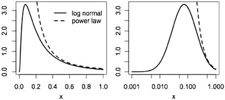

Log normal and power laws

Neighborhood:

the set of nodes to which a node is connected by an edge.

Node:

a point used to identify an object/entity in a graph. For example, we could consider individual areas of the brain as nodes. On a finer scale, we could consider individual neurons as nodes.

Path length:

the number of connected edges that must be traversed to travel between two nodes in a graph.

Power law:

used here as a probability law for which the frequency of an event declines as a power of its size. In graph theory, a power law may be used to define the degree distribution of a graph in which the frequency of nodes with a given degree falls off as a power function of the degree. This results in many nodes with a small degree and a few nodes with a very large degree (hubs).

Rich-club:

a higher-than-expected incidence of edges between hubs than between other nodes.

Small world graph:

a topological graph with high clustering and low average path length.

Spatially embedded graph:

a graph in which the spatial positions of the nodes (and, thus, the distances between them) are defined.

Topological or binary graph:

a graph defined solely in terms of the relations implied by its nodes and edges but with no additional attributes, such as a metric distance or spatial position, weights or any other measures. It can be represented by a simple connectivity matrix, with 0’s and 1’s for its entries, indicating non-connections or connections, respectively.

Box 2—Network Structure: Topological Versus Spatial Clustering

We distinguish between network properties that are purely topological, i.e., expressed only in terms of whether and what nodes are connected and perhaps their strength of connection, and those that depend also on other attributes, such as physical distance. To make the distinction clear, in the simple four node graph in Fig. 9, node b is equidistant topologically from nodes a and c since it is connected to each through a single edge. It is spatially closer to nodes c and d, however, even though d is further topologically from b (two edges distant). It is important to distinguish whether the connections between nodes in a graph depend only on topological considerations or whether spatial factors come into play, as well. Whether or not spatial or simply topological distance is related to the probability of a connection between nodes in a graph is an interesting question, because the answer can be informative as to the processes that generated the connections and thereby created the graph or variants with similar properties.

Fig. 9

A four-node graph in which nodes a and c are topologically equidistant from node b but nodes c and d are physically closer to node b

Spatial clustering is a notion expressing the fact that objects tend to bunch together in a limited region of space (and are perhaps also connected to one another), whereas network (or topological clustering) refers to the density of triangles in a network, without any reference to spatial embedding or positioning. In the definition of the SW, clustering is meant exclusively as network clustering, that is, as the density of the triangles, and has no relation to spatial clustering. Next we illustrate using simple examples that the two notions are entirely disconnected, i.e., high spatial clustering does not imply high network clustering and vice-versa. In Fig. 10a, we show a regular network embedded in space, which in this case is a simple ring. Every node is connected to the two closest nodes to their right and to their left. This is a network that is clearly clustered spatially (nodes connecting to their four closest neighbors). It has a network clustering coefficient C = 0.5. In Fig. 10b, we show exactly the same network (the same connectivity matrix), but the connected nodes are physically far apart in distance along the ring. Because the connectivity matrix has not changed, the network-clustering coefficient stays the same; however, the connected nodes are no longer clustered spatially. Thus, just because in a SW network we have large clustering, it does not imply that the nodes connected into triangles have to also be physically close to one another. The SW definition is simply topological; it does not imply any spatial embedding.

Fig. 10

Network clustering does not imply spatial clustering. A simple, regular network of 16 nodes embedded on a ring. In (a) the nodes are connected to their (spatially closest) four neighbors, whereas (b) shows the same network, therefore with identical network clustering, but without spatial clustering (the four neighbors of a node are at large distances from the node). (c) shows the US roadway (highway) network, in which nodes are spatially clustered (especially in densely populated areas), whereas (d) shows the United/Continental airline network, which has large network clustering but all triangles are between far-apart nodes. The SW property definition does not discriminate between (a) and (b) or (c) and (d)

Another, more realistic example comes from comparing the roadway network with the airline network. While both networks are embedded in space, they are drastically different. In the roadway network (formed by intersections of highways as nodes and edges as highway segments between intersections), there is strong spatial clustering (see Fig. 10c). Since there are no shortcuts in the roadway network, all network triangles are formed by nodes that are also physically close to one another, connected by road segments. By contrast, in the airline network (nodes are airports, edges are flights, Fig. 10d), which has a large network clustering coefficient (C = 0.34), the triangles are formed between physically distant nodes. There are typically no direct flights between physically close airports; instead we have to fly through network hubs to reach them.

The brain has some of both aspects: there is strong spatial and local network clustering between neighboring areas in the network, but there are also long-range links contributing to global clustering. Thus network clustering in this case is composed of both types of clustering: on one hand there are many triangles between closely spaced areas and, on the other, there are also many triangles in which at least two sides of the triangles are made of long-range connections.

References

Allman JM, Kaas JH (1971) Representation of the visual field in striate and adjoining cortex of the owl monkey (Aotus trivirgatus). Brain Res 35:89–106
Barabasi AL, Albert R (1999) Emergence of scaling in random networks. Science 286:509–512
Barone P, Batardiere A, Knoblauch K, Kennedy H (2000) Laminar distribution of neurons in extrastriate areas projecting to visual areas V1 and V4 correlates with the hierarchical rank and indicates the operation of a distance rule. J Neurosci 20:3263–3281
Bastos AM, Usrey WM, Adams RA, Mangun GR, Fries P, Friston KJ (2012) Canonical microcircuits for predictive coding. Neuron 76:695–711
Boccaletti S, Latora V, Moreno Y, Chavez M, Hwang DU (2006) Complex networks: structure and dynamics. Phys Rep 424:175–308
Braitenberg V, Schüz A (1998) Cortex: statistics and geometry of neuronal connectivity, 2nd edn. Springer, Berlin
Broder A, Kumar R, Maghoul F, Raghavan P, Rajagopalan S, Stata R, Tomkins A, Wiener J (2000) Graph structure in the web. Comput Netw 33:309–320
Buckner RL, Krienen FM (2013) The evolution of distributed association networks in the human brain. Trends Cogn Sci 17:648–665
Bullmore E, Sporns O (2012) The economy of brain network organization. Nat Rev Neurosci 13:336–349
Buzsaki G, Mizuseki K (2014) The log-dynamic brain: how skewed distributions affect network operations. Nat Rev Neurosci 15:264–278
Clark A (2013) Whatever next? Predictive brains, situated agents, and the future of cognitive science. Behav Brain Sci 36:181–204
Colizza V, Flammini A, Serrano MA, Vespignani A (2006) Detecting rich-club ordering in complex networks. Nat Phys 2:110–115
Csermely P, London A, Wu L-Y, Uzzi B (2013) Structure and dynamics of core/periphery networks. J Complex Netw 1:93–123
Csete M, Doyle J (2004) Bow ties, metabolism and disease. Trends Biotechnol 22:446–450
Dehaene S, Charles L, King JR, Marti S (2014) Toward a computational theory of conscious processing. Curr Opin Neurobiol 25C:76–84
Ercsey-Ravasz M, Markov NT, Lamy C, Van Essen DC, Knoblauch K, Toroczkai Z, Kennedy H (2013) A predictive network model of cerebral cortical connectivity based on a distance rule. Neuron 80:184–197
Felleman DJ, Van Essen DC (1991) Distributed hierarchical processing in the primate cerebral cortex. Cereb Cortex 1:1–47
Fries P (2005) A mechanism for cognitive dynamics: neuronal communication through neuronal coherence. Trends Cogn Sci 9:474–480
Gilbert CD, Li W (2013) Top-down influences on visual processing. Nat Rev Neurosci 14:350–363
Granovetter MS (1973) The strength of weak ties. Am J Sociol 78:1360–1380
Harriger L, van den Heuvel MP, Sporns O (2012) Rich club organization of macaque cerebral cortex and its role in network communication. PLoS One 7:e46497
Hilgetag CC, O’Neill MA, Young MP (1996) Indeterminate organization of the visual system. Science 271:776–777
Hill J, Inder T, Neil J, Dierker D, Harwell J, Van Essen D (2010) Similar patterns of cortical expansion during human development and evolution. Proc Natl Acad Sci USA 107:13135–13140
Honey CJ, Kotter R, Breakspear M, Sporns O (2007) Network structure of cerebral cortex shapes functional connectivity on multiple time scales. Proc Natl Acad Sci USA 104:10240–10245
Humphries MD, Gurney K (2008) Network ‘small-world-ness’: a quantitative method for determining canonical network equivalence. PLoS One 3:e0002051
Jones HE, Andolina IM, Grieve KL, Wang W, Salt TE, Cudeiro J, Sillito AM (2013) Responses of primate LGN cells to moving stimuli involve a constant background modulation by feedback from area MT. Neuroscience 246:254–264
Jouve B, Rosenstiehl P, Imbert M (1998) A mathematical approach to the connectivity between the cortical visual areas of the macaque monkey. Cereb Cortex 8:28–39
Kennedy H, Knoblauch K, Toroczkai Z (2013) Why data coherence and quality is critical for understanding interareal cortical networks. Neuroimage 80:37–45
Kitano H (2004) Biological robustness. Nat Rev Genet 5:826–837
Kitano H, Oda K (2006) Robustness trade-offs and host-microbial symbiosis in the immune system. Mol Syst Biol 2:2006 0022
Kleinberg J, Lawrence S (2001) Network analysis. The structure of the web. Science 294:1849–1850
Ma H, Zeng AP (2003) Reconstruction of metabolic networks from genome data and analysis of their global structure for various organisms. Bioinformatics 19:270–277
Ma H, Sorokin A, Mazein A, Selkov A, Selkov E, Demin O, Goryanin I (2007) The Edinburgh human metabolic network reconstruction and its functional analysis. Mol Syst Biol 3:135
Man K, Kaplan J, Damasio H, Damasio A (2013) Neural convergence and divergence in the mammalian cerebral cortex: from experimental neuroanatomy to functional neuroimaging. J Comp Neurol 521:4097–4111
Markov NT, Ercsey-Ravasz MM, Gariel MA, Dehay C, Knoblauch A, Toroczkai Z, Kennedy H (2011a) The tribal networks of the cerebral cortex. In: Chalupa LM, Berardi N, Caleo M, Galli-Resta L, Pizzorusso T (eds) Cerebral plasticity. MIT Press, Cambridge, MA, pp 275–290
Markov NT, Misery P, Falchier A, Lamy C, Vezoli J, Quilodran R, Gariel MA, Giroud P, Ercsey-Ravasz M, Pilaz LJ, Huissoud C, Barone P, Dehay C, Toroczkai Z, Van Essen DC, Kennedy H, Knoblauch K (2011b) Weight consistency specifies regularities of macaque cortical networks. Cereb Cortex 21:1254–1272
Markov NT, Ercsey-Ravasz M, Van Essen DC, Knoblauch K, Toroczkai Z, Kennedy H (2013a) Cortical high-density counter-stream architectures. Science 342:1238406
Markov NT, Ercsey-Ravasz MM, Lamy C, Ribeiro Gomes AR, Magrou L, Misery P, Giroud P, Barone P, Dehay C, Toroczkai Z, Knoblauch K, Van Essen DC, Kennedy H (2013b) The role of long-range connections on the specificity of the macaque interareal cortical network. Proc Nat Acad Sci USA 110:5187–5192
Markov NT, Vezoli J, Chameau P, Falchier A, Quilodran R, Huissoud C, Lamy C, Misery P, Giroud P, Barone P, Dehay C, Ullman S, Knoblauch K, Kennedy H (2014a) The anatomy of hierarchy: feedforward and feedback pathways in macaque visual cortex. J Comp Neurol 522:225–259
Markov NT, Ercsey-Ravasz MM, Ribeiro Gomes AR, Lamy C, Magrou L, Vezoli J, Misery P, Falchier A, Quilodran R, Gariel MA, Sallet J, Gamanut R, Huissoud C, Clavagnier S, Giroud P, Sappey-Marinier D, Barone P, Dehay C, Toroczkai Z, Knoblauch K, Van Essen DC, Kennedy H (2014b) A weighted and directed interareal connectivity matrix for macaque cerebral cortex. Cereb Cortex 24:17–36
McAlonan K, Cavanaugh J, Wurtz RH (2006) Attentional modulation of thalamic reticular neurons. J Neurosci 26:4444–4450
McAlonan K, Cavanaugh J, Wurtz RH (2008) Guarding the gateway to cortex with attention in visual thalamus. Nature 456:391–394
Modha DS, Singh R (2010) Network architecture of the long-distance pathways in the macaque brain. Proc Natl Acad Sci USA 107:13485–13490
Natarajan M, Lin KM, Hsueh RC, Sternweis PC, Ranganathan R (2006) A global analysis of cross-talk in a mammalian cellular signalling network. Nat Cell Biol 8:571–580
Newman MEJ (2010) Networks: an introduction. Oxford University Press, Oxford
Oh SW, Harris JA, Ng L, Winslow B, Cain N, Mihalas S, Wang Q, Lau C, Kuan L, Henry AM, Mortrud MT, Ouellette B, Nguyen TN, Sorensen SA, Slaughterbeck CR, Wakeman W, Li Y, Feng D, Ho A, Nicholas E, Hirokawa KE, Bohn P, Joines KM, Peng H, Hawrylycz MJ, Phillips JW, Hohmann JG, Wohnoutka P, Gerfen CR, Koch C, Bernard A, Dang C, Jones AR, Zeng H (2014) A mesoscale connectome of the mouse brain. Nature 508:207–214
Opsahl T, Colizza V, Panzarasa P, Ramasco JJ (2008) Prominence and control: the weighted rich-club effect. Phys Rev Lett 101:168702
Preuss TM (2011) The human brain: rewired and running hot. Ann N Y Acad Sci 1225(Suppl 1):E182–E191
Rosa MG, Tweedale R (2005) Brain maps, great and small: lessons from comparative studies of primate visual cortical organization. Philos Trans R Soc Lond B Biol Sci 360:665–691
Sherwood CC, Bauernfeind AL, Bianchi S, Raghanti MA, Hof PR (2012) Human brain evolution writ large and small. Prog Brain Res 195:237–254
Siganos G, Tauro SL, Faloutsos M (2006) Jellyfish: a conceptual model for the as internet topology. J Commun Netw 8:339–350
Supper J, Spangenberg L, Planatscher H, Drager A, Schroder A, Zell A (2009) BowTieBuilder: modeling signal transduction pathways. BMC Syst Biol 3:67
Tauro SL, Palmer C, Siganos G, Faloutsos M (2001) A simple conceptual model for the Internet topology. In: Global Telecommunications Conference, 2001. GLOBECOM’01. IEEE, pp 1667–1671
van den Heuvel MP, Kahn RS, Goni J, Sporns O (2012) High-cost, high-capacity backbone for global brain communication. Proc Natl Acad Sci USA 109:11372–11377
Van Essen DC, Dierker DL (2007) Surface-based and probabilistic atlases of primate cerebral cortex. Neuron 56:209–225
Van Essen DC, Felleman DJ, DeYoe EA, Olavarria J, Knierim J (1990) Modular and hierarchical organization of extrastriate visual cortex in the macaque monkey. Cold Spring Harb Symp Quant Biol 55:679–696
Wang W, Slotine JJ (2005) On partial contraction analysis for coupled nonlinear oscillators. Biol Cybern 92:38–53
Wang W, Jones HE, Andolina IM, Salt TE, Sillito AM (2006) Functional alignment of feedback effects from visual cortex to thalamus. Nat Neurosci 9:1330–1336
Wang Q, Sporns O, Burkhalter A (2012) Network analysis of corticocortical connections reveals ventral and dorsal processing streams in mouse visual cortex. J Neurosci 32:4386–4399
Watts DJ, Strogatz SH (1998) Collective dynamics of ‘small-world’ networks. Nature 393:440–442
Young MP (1992) Objective analysis of the topological organization of the primate cortical visual system. Nature 358:152–155
Young MP (1993) The organization of neural systems in the primate cerebral cortex. Proc R Soc Lond B Biol Sci 252:13–18
Zador AM, Dubnau J, Oyibo HK, Zhan H, Cao G, Peikon ID (2012) Sequencing the connectome. PLoS Biol 10:e1001411
Zhou S, Mondragon RJ (2004) The rich-club phenomenon in the internet topology. IEEE Commun Lett 8:180–182
Zingg B, Hintiryan H, Gou L, Song MY, Bay M, Bienkowski MS, Foster NN, Yamashita S, Bowman I, Toga AW, Dong HW (2014) Neural networks of the mouse neocortex. Cell 156:1096–1111
Acknowledgments
This work was supported by FP6-2005 IST-1583 (HK); FP7-2007 ICT-216593 (HK); ANR-11-BSV4-501 (HK); LABEX CORTEX (ANR-11-LABX-0042) of Université de Lyon, within the program “Investissements d’Avenir” (ANR-11-IDEX-0007) operated by the French National Research Agency (ANR) (HK); PN-II-RU-TE-2011-3-0121, FP7-PEOPLE-2011-IIF-299915 (MER); in part, by grant FA9550-12-1-0405 from the U.S. Air Force Office of Scientific Research and Defense Advanced Research Projects Agency (ZT).
Author information
Authors and Affiliations
Corresponding author
Editor information
Editors and Affiliations
Rights and permissions
Open Access This chapter is distributed under the terms of the Creative Commons Attribution-Noncommercial 2.5 License (http://creativecommons.org/licenses/by-nc/2.5/) which permits any noncommercial use, distribution, and reproduction in any medium, provided the original author(s) and source are credited.
The images or other third party material in this chapter are included in the work’s Creative Commons license, unless indicated otherwise in the credit line; if such material is not included in the work’s Creative Commons license and the respective action is not permitted by statutory regulation, users will need to obtain permission from the license holder to duplicate, adapt or reproduce the material.
Copyright information
© 2016 The Author(s)
About this chapter
Cite this chapter
Knoblauch, K., Ercsey-Ravasz, M., Kennedy, H., Toroczkai, Z. (2016). The Brain in Space. In: Kennedy, H., Van Essen, D., Christen, Y. (eds) Micro-, Meso- and Macro-Connectomics of the Brain. Research and Perspectives in Neurosciences. Springer, Cham. https://doi.org/10.1007/978-3-319-27777-6_5
Download citation
DOI: https://doi.org/10.1007/978-3-319-27777-6_5
Published:
Publisher Name: Springer, Cham
Print ISBN: 978-3-319-27776-9
Online ISBN: 978-3-319-27777-6
eBook Packages: Biomedical and Life SciencesBiomedical and Life Sciences (R0)