LS-RAPID Manual with Video Tutorials

Abstract

LS-RAPID is an integrated simulation model capable of capturing the entire landslide process starting from a state of stability to landslide initiation and movement to the mass deposition. This paper provides an overview of the use of LS-RAPID to simulate landslide case histories around the world, provides a manual for readers to begin using the program for simulations, and describes the use of the program for several models. Specific steps to use the basic and advanced features in LS-RAPID are provided within the paper. Additionally, video tutorials are provided to supplement the descriptive steps provided in this paper. These tutorials are developed to focus on individual aspects of the program. The paper concludes with three tutorials that provide a complete walk-through of the use of the program from start to finish. These tutorials are for (1) an example of a rainfall-induced failure, (2) an example of an earthquake-induced failure, and (3) the case study of the Atami debris flow. The Atami debris flow illustrates the ability of LS-RAPID to reproduce reliable results associated with the initiation and runout motions of the observed failure.

1 Chapter 1: Introduction

LS-RAPID was developed by Sassa et al. (2010) as an integrated landslide simulation model that aims to model the whole process of a landslide including the stable state, failure stage, post-failure shear strength reduction, landslide motion, steady state condition and the mass deposition stage. This model is an upgrade to a numerical simulation model for landslides proposed by Sassa (1988).

In principle, the LS-RAPID model is intended to integrate the initiation mechanism and the behavior motion of a landslide from the initial failure of the slope (stability analysis) to the mobilization and expansion of landslide materials (dynamic analysis) to the deposition stage. The user can also perform partial analysis for a landslide model, for example, only simulate the motion simulation, or conduct full mode simulation that includes initiation, motion and expansion. Within the LS-RAPID model, changes in the behavior of the landslide can be captured when the triggering factors are initiated.

The LS-RAPID model can accommodate landslide simulations for failures induced by rainfall as well as earthquakes, For rainfall-induced landslides, simulations can be undertaken by inputting either the pore water pressure ratio or using hourly rainfall data time series. For earthquake-induced landslides, the simulation can be conducted using the static mode with a seismic coefficient, cyclic loading or seismic loading provided from an earthquake peak ground acceleration time series record. The program can also consider combined triggering factors, that involve both rainfall and earthquake conditions applied simultaneously. The application is based on the data that is inputted into the simulation.

1.1 Example Case Studies

LS-RAPID has been applied in the study of numerous landslide cases around the world. The use of LS-RAPID in some case studies was integrated with laboratory tests through undrained dynamic loading ring shear apparatus to obtain the dynamic and residual shear strength of soils, i.e., post-failure state during large shear displacements and the pore-water pressure conditions as input parameters. Meanwhile, other studies have used approximate parameters estimated from back analysis, results of peak shear strength and static geotechnical tests.

Table 1 present a list of case studies in which LS-RAPID models were utilized. These case studies involve landslides triggered by rainfall or earthquake and have already been published in journals, chapter books and conference proceedings. The relevant references for additional information about the case study are also provided.

Table 1 Application of LS-RAPID in landslide case studies around the world

2 Theoretical Background

2.1 Basic Principle and Governing Equations

The concept of the LS-RAPID model was established by considering that the unstable slope consists of the landslide mass and stable ground in a form of a vertical imaginary column (Fig. 1). The forces acting within this moving landslide mass include the weight of the column (W), the vertical seismic force (F_v), horizontal seismic forces in the x- and y-directions (F_x and F_y, respectively), lateral pressure acting both on side walls (P), shear resistance acting on the bottom and interface with the stable ground (R), the normal stress acting on the bottom (N) from the stable ground as a reaction to the normal component of the self-weight, and the pore pressure acting on the bottom (U).

Fig. 1

Column element within a moving landslide mass as basis of the LS-RAPID model (Sassa et al. 2010)

Following Newton’s laws of motion, the acceleration (a) of the landslide mass (m) will be the result of the sum of driving forces (self-weight and seismic force), shear resistance (R) and the change in lateral pressure (P), denoted as:

$$a\cdot m=\left(W+{F}_{v}+{F}_{x}+{F}_{y}\right)+\left(\frac{\partial {P}_{x}}{{\partial }_{x}}\Delta x+\frac{\partial {P}_{x}}{{\partial }_{y}}\Delta y\right)+R$$

(1)

However, the effects of forces N and U that are projected in the upward direction of the maximum slope line contribute before the motion and work during the motion against the direction of the landslide mass movement. All stresses and displacements are projected and calculated in to the horizontal plane (Sassa 1988).

The left side of Eq. (1) is then projected in to the x-, y- and z-directions by considering the flows in and out of the column element with constant average velocity as shown below:

$${a}_{x}=\frac{\partial {u}_{0}}{\partial t}+{u}_{0}\frac{\partial {u}_{0}}{\partial x}+{v}_{0}\frac{\partial {u}_{0}}{\partial y}+{w}_{0}\frac{\partial {u}_{0}}{\partial z}$$

(2)

$${a}_{y}=\frac{\partial {v}_{0}}{\partial t}+{u}_{0}\frac{\partial {v}_{0}}{\partial x}+{v}_{0}\frac{\partial {v}_{0}}{\partial y}+{w}_{0}\frac{\partial {v}_{0}}{\partial z}$$

(3)

The velocity along z-direction is neglected since the simulation is typically conducted to understand the mechanism and motion behavior of the moving landslide mass in area.

To represent the moving landslide mass, the LS-RAPID model uses the soil flow to x-direction per unit width as flux M and the soil flow to y-direction per unit width as flux N, that are both associated with the velocities and the height of soil column (h). They are expressed as:

$$M = u_{0} \cdot h\;{\text{and}}\;N = v_{0} \cdot h$$

(4)

Therefore, the left side of Eq. (1) will become Eqs. (5) and (6) below:

$$\frac{1}{h}\left\{\frac{\partial M}{\partial t}+\frac{\partial }{\partial x}\left({u}_{o}M\right)+\frac{\partial }{\partial y}\left({v}_{o}M\right)\right\}=\left(W+{F}_{v}+{F}_{x}+{F}_{y}\right)+\left(\frac{\partial {P}_{x}}{{\partial }_{x}}\Delta x+\frac{\partial {P}_{y}}{\partial y}\Delta y\right)+R$$

(5)

$$\frac{1}{h}\left\{\frac{\partial N}{\partial t}+\frac{\partial }{\partial x}\left({u}_{o}N\right)+\frac{\partial }{\partial y}\left({v}_{o}N\right)\right\}=\left(W+{F}_{v}+{F}_{x}+{F}_{y}\right)+\left(\frac{\partial {P}_{x}}{{\partial }_{x}}\Delta x+\frac{\partial {P}_{y}}{\partial y}\Delta y\right)+R$$

(6)

As a result of the moving landslide mass, the right side of Eq. (1) consists of:

• the gravity term, $\left(W+{F}_{v}+{F}_{x}+{F}_{y}\right)$

• the pressure term, $\frac{\partial {P}_{x}}{{\partial }_{x}}\Delta x+\frac{\partial {P}_{x}}{{\partial }_{y}}\Delta y$, and

• the shear resistance per unit area on x–y plane, R.

The gravity term, by including the seismic acceleration, is projected to x- and y-directions and associated with the vertical seismic acceleration (g × K_v) and horizontal seismic acceleration acting on x- (g × K_x) and y-directions (g × K_y), as stated below (Fig. 2):

Fig. 2

Projection of (left) gravity and vertical seismic force and (right) gravity and horizontal seismic force

$$1 + {\rm{K}}_{{\rm{v}}} \;{\rm{works}}\;{\rm{in}}\;{\rm{the}}\;{\rm{x - direction:}}\;g\frac{{{\rm{tan}}{\alpha} }}{{q + 1}}\left( {1 + K_{v} } \right)$$

(7)

$$1 + {\rm{K}}_{{\rm{v}}} \;{\rm{works}}\;{\rm{in}}\;{\rm{the}}\;{\rm{y - direction:}}\;g\frac{{{\rm{tan}}{\beta} }}{{q + 1}}\left( {1 + K_{v} } \right)$$

(8)

$${\rm{For}}\;{\rm{horizontal}}\;{\rm{acceleration}}\;{\rm{along}}\;{\rm{x:}}\;g\;K_{x} \;cos^{2} \;\alpha$$

(9)

$${\rm{For}}\;{\rm{horizontal}}\;{\rm{acceleration}}\;{\rm{along}}\;{\rm{y:}}\;g\;K_{y} \;cos^{2} \;\alpha $$

(10)

The pressure term is the difference of the lateral pressure acting on both sides of columns in the x- and y-directions (Fig. 3), where the lateral pressure is expressed using the lateral earth pressure ratio (k), as shown in Eqs. (11) and (12).

Fig. 3

Lateral pressure acting on a soil column

$$\left(1+{K}_{v}\right)\cdot k\cdot g\cdot \frac{\partial h}{\partial x}(\mathrm{x}-\mathrm{ direction})$$

(11)

$$\left(1+{K}_{v}\right)\cdot k\cdot g\cdot \frac{\partial h}{\partial y}(\mathrm{y}-\mathrm{ direction})$$

(12)

According to Sassa (1988), shear resistance per unit area on the x–y plane is acting in the direction opposite to the direction of the movement of the landslide mass. The components of shear resistance in the x- and y- directions are given by Eqs. (13) and (14), respectively:

$$\frac{g}{{\left(q+1\right)}^{1/2}}\,\cdot \,\frac{{u}_{o}}{{\left({u}_{o}^{2}+{v}_{o}^{2}+{w}_{o}^{2}\right)}^{1/2}}\,\left\{{h}_{c}\left(q+1\right)+\left(1-{r}_{u}\right)\,h\mathrm{tan}{\varphi }_{a}\right\}$$

(13)

$$\frac{g}{{\left(q+1\right)}^{1/2}}\,\cdot \,\frac{{v}_{o}}{{\left({u}_{o}^{2}+{v}_{o}^{2}+{w}_{o}^{2}\right)}^\frac{1}{2}}\,\left\{{h}_{c}\left(q+1\right)+\left(1-{r}_{u}\right)\,h\mathrm{tan}{\mathrm{\varphi }}_{\mathrm{a}}\right\}$$

(14)

where w_o = −(u_o tan$\alpha$ + v_o tan$\beta$), while the effect of the apparent friction coefficient (tan$\phi_{\rm{a}}$), the pore pressure ratio (r_u) and cohesion in the unit of height (h_c) are dependent on the shear strength reduction stages.

Based on the deductions provided above, Eq. (1) can be completely expressed into the x- and y-directions as given by Eqs. (15) and (16), respectively below:

$$\frac{\partial M}{\partial t}+\frac{\partial }{\partial x}\left({u}_{o}M\right)+\frac{\partial }{\partial y}\left({v}_{o}M\right)=g\,h\,\left\{\frac{\mathrm{tan}\alpha }{q+1}\left(1+{K}_{v}\right)+{K}_{x}\,{\mathit{cos}}^{2}\alpha \right\}-\left(1+{K}_{v}\right)\,k\,g\,h\,\frac{\partial h}{\partial x}-\frac{g}{{\left(q+1\right)}^{1/2}}\,\cdot \,\frac{{u}_{o}}{{\left({u}_{o}^{2}+{v}_{o}^{2}+{w}_{o}^{2}\right)}^{1/2}}\,\left\{{h}_{c}\left(q+1\right)+\left(1-{r}_{u}\right)\,h\mathrm{tan}{\varphi }_{a}\right\}$$

(15)

$$\frac{\partial N}{\partial t}+\frac{\partial }{\partial x}\left({u}_{o}N\right)+\frac{\partial }{\partial y}\left({v}_{o}N\right)=g\,h\,\left\{\frac{\mathrm{tan}\beta }{q+1}\left(1+{K}_{v}\right)+{K}_{x}\,{\mathit{cos}}^{2}\beta \right\}-\left(1+{K}_{v}\right)\,k\,g\,h\,\frac{\partial h}{\partial y}-\frac{g}{{\left(q+1\right)}^{1/2}}\,\cdot \,\frac{{v}_{o}}{{\left({u}_{o}^{2}+{v}_{o}^{2}+{w}_{o}^{2}\right)}^{1/2}}\,\left\{{h}_{c}\left(q+1\right)+\left(1-{r}_{u}\right)\,h\mathrm{tan}{\varphi }_{a}\right\}$$

(16)

If it is assumed that the total density of the landslide mass does not change during motion, i.e., the sum of landslide mass flowing into a column (M, N) is balanced by the change in the height of the soil column, then:

$$\frac{\partial h}{\partial t}+\frac{\partial M}{\partial x}+\frac{\partial N}{\partial y}= 0$$

(17)

Equations (15) to (17) were generated for both the processes of the landslide initiation and its motion. The variables in these equations are provided in Table 2.

Table 2 Variables in the equations for LS-RAPID

The values of $\phi_{\rm{a}}$, h_c, and r_u vary across three conditions: (i) pre-failure state before shear displacement (start of shear reduction), (ii) transient state after failure up to a steady state, and (iii) steady state (residual state) after the end of strength reduction. The lateral earth pressure ratio in Eqs. (15) and (16) is expressed using Jaky’s equation (Sassa 1988) as follows:

$$k=1-\mathrm{sin}{\phi }_{ia}$$

(18)

$$\mathrm{tan}{\varphi }_{ia}= \frac{\left(c+\left(\sigma -u\right)\mathrm{tan}{\phi }_{i}\right)}{\sigma }$$

(19)

where tan $\phi_{\rm{ia}}$ is the apparent friction coefficient within the landslide mass and tan $\phi_{\rm{i}}$ is the effective friction coefficient within the landslide mass, which is not always the same as the effective friction coefficient during motion on the sliding surface ($\phi_{\rm{m}}$).

The value of k differs depending on whether the sample is in the liquefied state or in the rigid state. It can be expressed as follows:

• Liquefied state, $\sigma$ = u, c = 0, sin$\phi_{\rm{ia}}$ = 0 and k = 1.0

• Rigid state, c is significant, sin$\phi_{\rm{ia}}$ = 1.0 and k = 0

An increase in the pore water pressure within a slope due to rainfall, rises of the groundwater table, and/or earthquakes may affect stresses, particularly along the susceptible sliding (slip) surface of a slope. A landslide occurs when the effective stress path in the stress-shear graph moves from the initial stress condition and reaches the peak failure line ($\phi$_p). Volume reduction will take place as shear displacement progresses in saturated soils after failure as a result of grain crushing/soil particle breakage and the generation of excess pore water pressures.

The stress path will travel down along the failure line during motion of the landslide mass with certain friction ($\phi$_m) angle until it reaches the steady (residual) state condition. The steady-state condition describes failure of the sample when there is no further grain crushing occurring at a constant value of pore water pressure with unchanged volume of the samples. Under this condition, only shear displacement occurs under a condition of constant shear resistance, which is known as the steady-state shear resistance. It is described by the following formula:

$${\tau }_{ss}= {\sigma }_{ss}\mathrm{tan}{\phi }_{m}= {\sigma }_{0} \mathrm{tan}{\phi }_{a(ss)}$$

(20)

where $\tau$_ss and $\sigma$_ss are the shear and normal stresses, respectively, at the steady-state condition and tan$\phi$_a(ss) is the associated apparent friction coefficient. Thus, the apparent friction coefficient can be expressed as the ratio of steady-state shear resistance ($\tau$_ss) and the initial normal stress acting on the sliding surface ($\sigma$₀), which corresponds to the total normal stress ($\sigma$) due to the in-situ soil weight in the simulation.

$$\mathrm{tan}{\phi }_{a(ss)}= \frac{{\tau }_{ss}}{\sigma }$$

(21)

Ideally, from the ring shear tests, the apparent friction coefficient (tan $\phi$_a(ss)) can be obtained by knowing the steady-state shear resistance ($\tau$_ss) and the normal stress ($\sigma$). In addition, the concept of shear strength reduction during the progression of shear displacement from the pre-failure state to steady-state motion is shown in Fig. 4 (Sassa et al. 2010). The transient state from the peak state to the steady-state was observed when conducting ring shear tests (Sassa and Dang 2018). As an example of this shear-displacement relationship, Fig. 5 shows the shear strength reduction in terms of shear resistance (in kPa) with respect to the shear displacement (in mm, plotted in logarithmic scale) within a sample during a undrained cyclic loading test using a ring shear apparatus.

Fig. 4

Shear strength reduction during the progression of shear displacement (Sassa et al. 2010)

Fig. 5

Shear stress and shear displacement relationship in an undrained cyclic loading test on the Tertiary Sand (Sassa and Dang 2018)

The shear strength reduction within the landslide mass consists of four stages, which are: (i) initial state, (ii) pre-failure state, (iii) transient state, and (iv) steady-state. In the initial state, soil stability is obtained under the peak friction coefficient (tan ϕ_p). The pre-failure state occurs when shear resistance reaches the peak friction coefficient due to rainfall, rises in the groundwater table, earthquakes or the combination of these factors. The critical shear displacement in the pre-failure state (stated as DL) indicates failure of soils and the occurrence of landslide. The transient state take place during the transition from failure point to the steady-state condition (Fig. 4). Pore pressure generation and shear strength reduction will occur during the transient state as a result of grain crushing, landslide mass mobilization and shear strength reduction. The critical shear displacement from the transition state to steady state condition is indicated by the end of shear reduction (stated as DU; Fig. 5). The friction coefficient represents the shear resistance during shear loading in the constant normal stress (Δ$\sigma$ = 0).

According to the description of the shear strength reduction stages above, the shear displacement (D), the friction coefficient (tan $\phi$), and the effect of pore pressure ratio (r_u) can be expressed in each stage as follows:

• Initial deformation stage before failure (D < DL):

tan $\phi_{\rm{a}}$ = tan $\phi_{\text{p}}$

c = c_p

r_u = c_u

• Transient state after failure (DL ≤ D ≤ DU):

  $$ \tan \varphi_{a} = \tan \varphi_{p} - \frac{\log D - \log DL}{{\log DU - \log DL}}\left( {\tan \varphi_{p} - \tan \varphi_{a(ss)} } \right) $$
  $$ c = c_{p} \;\left( {1 - \frac{\log D - \log DL}{{\log DU - \log DL}}} \right) $$
  $$ r_{u} = r_{u} \; \cdot \;\frac{\log DU - \log D}{{\log DU - \log DL}} $$

• Steady-state motion (D > DU):

tan $\phi_{\text{a}}$ = tan $\phi_{{\rm{a}}({\rm{ss}})}$

c = 0

r_u = 0

3 User Manual

3.1 Simulation Overview

The steps involved in simulating a landslide using LS-RAPID are summarized in Fig. 6. The simulation begins with the establishment of settings that will allow viewing of the topography being modeled. Data related to the topography is then inputted into the program. There are two paths that can be taken to do so. In the first, a topography control point is established using which the topography is estimated. Alternatively, the mesh data for the topography is directly inputted and the control point is then established.

A process similar to the topography mesh and control point may be used to simulate the sliding surface and its associated control point. However, if a sliding surface mesh and/or control point are not available, the sliding surface for the landslide may be determined through several other means within LS-RAPID. Specifically, the sliding surface can be established using the ellipsoidal parameters or by modeling the filling and excavation processes. This information can be then be converted into mesh data that establishes the sliding surface for the simulation.

The final steps before the start of the simulation will involve the configuration of various settings within LS-RAPID. In particular, it will be necessary to input the triggering factors (rainfall events, earthquake events or both), properties of the soils present in the landslide mass and sliding surface and properties of water. This chapter will contain detailed information about the specific steps necessary to simulate a landslide using LS-RAPID. Figure 6 also indicates video tutorials that are available for the simulation process. It is noted that depending on the available information and specific details of the landslide being simulated, several of the steps provided here may not be applicable. Interested users may also need to perform additional steps, not necessarily described in this section, to collect and format the data available for the purposes of their simulations.

Fig. 6

Flowchart containing steps for simulation using LS-RAPID

3.2 Preparation of the Digital Elevation Data Using DEMmake

Digital elevation models (DEMs) generally provide latitude, longitude and elevation information in an (x,y,z) format within a text file. Before this information can be used in simulations in LS-RAPID, it will be necessary to convert the text file into elevation mesh data. LS-RAPID is accompanied by a software, an Excel Spreadsheet titled, “DEMmake,” that allows the user to easily convert the DEM text file into the required elevation mesh data for the LS-RAPID input. A tutorial of the use of the DEMmake program, is titled, “1. Preparation of DEM Data.” A brief summary of the steps is provided below:

• 1. Open the DEMmake Excel program. The use of DEMmake will require that use of macros within Excel is enabled. If this is disabled, the setting can be changed by allowing content in the warning that appears at the top of the Excel file when DEMmake is opened. Macros can also be enabled by going to the “File” menu in Excel and selecting “Options.” From the dialog box titled, “Excel Options,” select “Trust Center” and then click the button for “Trust Center Settings” on the right. In the options on the left side, select “Marco settings” and then select the “Enable all macros (not recommended; potential dangerous code can run)” option. The opened DEMmake program will resemble the contents in Fig. 7.

  Fig. 7

  

  Screenshot of DEMmake program when opened with macros enabled

• 2. Using the “Select Text-file” button at the top left of the DEMmake program, the text file containing the (x,y,z) coordinates should be selected. The data in the text file should be delineated (or separated) by commas or spaces for its use in the DEMmake program.

• 3. Automatically compute the range (minimum and maximum values) of the x-, y- and z-coordinates using the “Get Coordinate range information” button in the bottom right. The ranges for the x- and y-coordinates will be necessary in Step 4.

• 4. Transfer the ranges for the x- and y-coordinates (from Step 3) into the green “Grid” cells in the center of the DEMmake program. The interval of the x- and y- coordinates will then need to be specified in the “Pitch” column. Specifically, a pitch of 5.0 in the row containing x-coordinate information and a pitch of 10.0 in the row containing y-coordinate information would indicate that the difference between adjacent x-coordinates will be equal to 5.0, while the distance between adjacent y-coordinates is equal to 10.0. Based on the range of the coordinates and the pitch used, the number of grids will be automatically calculated. The user is cautioned against inputting any numbers in the grayed cells indicating the number of grids.

• 5. Now that all of the input information has been entered into the DEMmake program, it will be possible to generate the DEM data needed for the LS-RAPID simulation. To do so, click on the “Generate DEM” button. The DEM data that is generated will be stored in a separate Worksheet of the DEMmake Excel file. Specifically, the data will be found in the sheet titled, “DEMdata,” as shown in the screenshot in Fig. 8. In the cases when the control point was located at distance greater than the value specified in Step 5 from the grid point, the elevation (z-coordinate) information will not be provided in the DEM data generated. If an elevation value is necessary at a particular point, but not available in the DEMdata sheet, it may be necessary to make adjustments in Step 5 (by increasing the distance specified) and repeat this step.

  Fig. 8

  

  Screenshot of the DEMdata worksheet of the DEMmake program

The DEM data associated with the simulation area of interest for the LS-RAPID model should then be selected from the DEMdata sheet. When determining the Calculation Area for the LS-RAPID (as will be discussed later in this section), it will be necessary to know the number of mesh. This is equal to one less than the number of grids for the selected area. It is also possible to set-up the Simulation Area prior to generating the DEM data using DEMmake, as will be explained in the “Initial Topography” subsection later in this chapter. If this process is adapted, the number of grids will be automatically calculated by LS-RAPID.

3.3 Preparation of the Digital Elevation Data Using DEMmake

When LS-RAPID is first opened, there will be no information regarding the topography or details about the settings for the simulation. In this section, details regarding inputting this information to the program will be provided.

3.3.1 Simulation Area

The steps to establish the simulation area within LS-RAPID are provided below. A video tutorial titled, “2. Initial Setting of Topography 1” also describes this steps for interested users to follow.

• 1. Locate the “Flow” panel on the left side of the LS-RAPID program, as shown in Fig. 9. Within this panel, expand Section “1: Mesh” and click on the “Simulation area” button. A window titled, “Setting of simulation area and input-data type” will open and look similar to that shown in Fig. 10.

  Fig. 9

  

  Screenshot of the flow panel (in red box) in LS-RAPID

  Fig. 10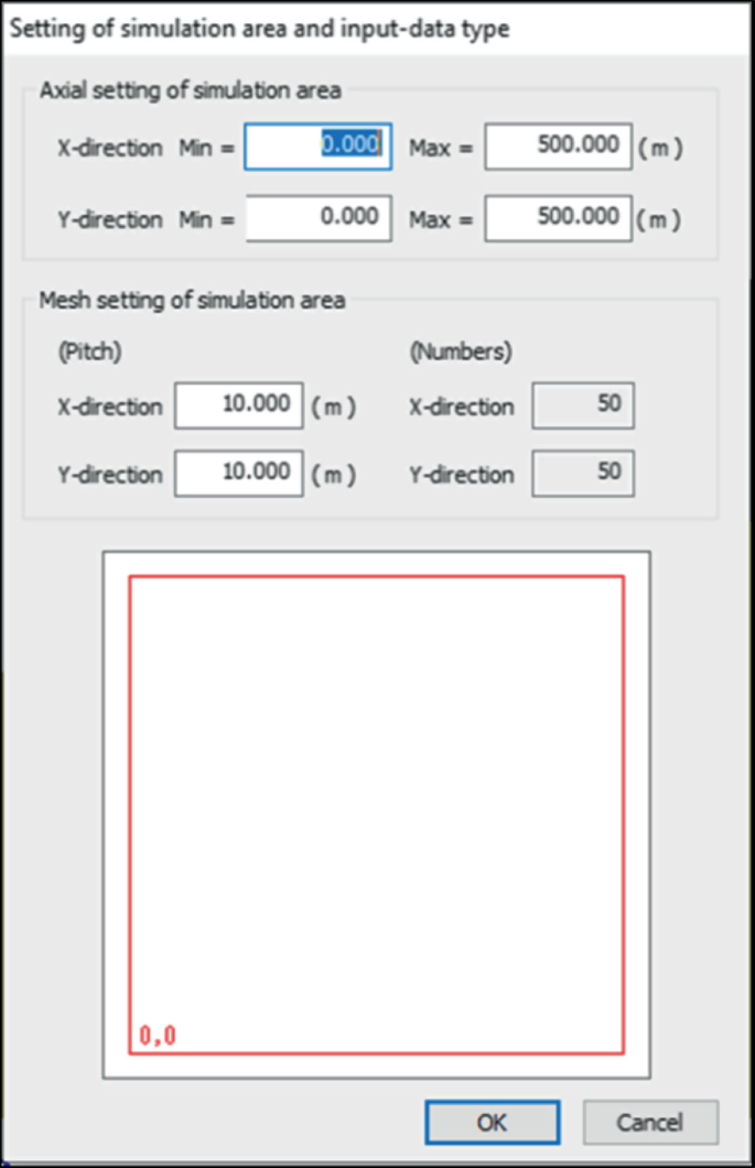

  

  Screenshot of the setting of simulation area and input-data type window

• 2. The minimum and maximum values of the x- and y-coordinates associated with the calculation area should be inputted in the top section titled, “Axial Setting of Calculation Area,” as shown in Fig. 10. LS-RAPID will allow inputs between −999,999.999 and +999,999.999 m.

• 3. The second component of this window is the “Mesh Setting of Calculation Area” section. This section is used to input the pitch for the x- and y-directions. As with the DEMmake program, LS-RAPID will then automatically calculate the number of grids in both directions using the ranges from Step 2 and the input pitch values. LS-RAPID allows between 2 and 9999 numbers of mesh and pitch values between 0.001 and 999,999.99.

• 4. The simulation area along with the grid developed will be illustrated in the bottom part of the Setting of Simulation Area and Input-Data Type Window. In particular, the red box will delineate the extents of the calculation area, while the gray lines will indicate the location of the grid lines.

• 5. Upon clicking “Ok,” the calculation area will be displayed in the right panel of the LS-RAPID program, as shown in Fig. 11.

  Fig. 11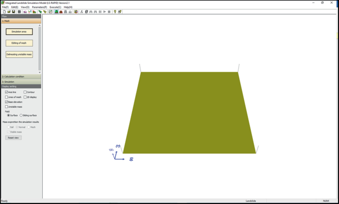

  

  Screenshot of calculation area

3.3.2 Editing Mesh

3.3.2.1 Slope Surface

As noted in the flow chart in Fig. 6, the topography can be established in LS-RAPID using one of two different approaches. In the first approach, the topography control points are added and a mesh is generated while in the second, the mesh is directly added into the program. The steps to generate a mesh from the topography control points are summarized below:

• 1. From the “Edit” menu in the toolbar at the top of the program, select the “Editing of Control Point” option, as illustrated in the screenshot in Fig. 12.

  Fig. 12

  

  Screenshot of edit menu in toolbar

• 2. The control points can then be manually entered into the appropriate tab in the window that opens titled, “Editing of Control Point.” This window is presented in Fig. 13. For this section, the control points would be entered into the “Slope Surface Elevation” tab. Once the data has been entered into the tab, Click “Ok.”

  Fig. 13

  

  Screenshot of the editing control point window

• 3. In lieu of manual entry as described in Step 2, a text file containing the control point data may be imported into LS-RAPID. To do this, from the “File” menu in the Toolbar, select the “Read text data file” option. Next, click on the “Read (Ground Elevation) Control Point” to select the text file that contains the appropriate control point data. The options available in the “File” menu are shown in Figure 14. It is noted that the text file containing the control point data should be in a CSV format and separated by either a space, tab or comma to be properly read by LS-RAPID.

  Fig. 14

  

  File menu options for inputting control point data text file

• 4. Once the control points have been inputted as described in Step 2 or have been imported following the instructions in Step 3, the results in the viewing panel will be similar to that shown in Fig. 15.

  Fig. 15

  

  Viewing panel with topography control point data

• 5. The control points will now need to be converted into a mesh. This is accomplished by selecting the “Transfer control point data to mesh data” option in the “Edit” menu from the toolbar. This is shown in Fig. 12. The mesh topography based on the control point data will then be displayed in the viewing panel. An example is shown in Fig. 16. If necessary, control points can be edited using either Step 2 or Step 3 before.

  Fig. 16

  

  Example of topography mesh in viewing panel

Topography mesh data can also be directly added to LS-RAPID without the use of the control points using one of two different methods. The steps to both methods are summarized below:

Method 1: Importing Mesh Data into LS-RAPID.

• 1. The mesh data can be imported into LS-RAPID if a text file containing the data is available. To do so, select the “Read text data file” option from the “File” menu shown in Fig. 14. Next, click on the “Read (ground elevation) mesh data” option.

• 2. The text file containing the topography mesh data should be selected and the window closed. The result will be a topography mesh similar to that shown in Fig. 16.

Method 2: Inputting Mesh Data into LS-RAPID.

The steps for this process are summarized below, but can also be found in the video tutorial titled, “3. Initial Setting of Topography 2.”

• 1. Mesh data is added into the calculation area using the “Editing of Mesh” button in the “Flow” Panel under Section “1:Mesh,” as seen in Fig. 9.

• 2. A window titled, “Editing of mesh” will open containing several sections and tabs to input data. This window is shown in Fig. 17. The “Change header” section should be used to select the type of mesh representation provided in the rows and columns where data will be inputted. Specifically, when “Index” is selected, the mesh is represented with the numbers associated with the grid lines in the calculation area. Alternatively, the “Position” option will give the x- and y-coordinates of the calculation area where elevation data will be inputted. The one most appropriate for the simulation at hand should be selected.

  Fig. 17

  

  Screenshot of the editing of mesh window

• 3. The “Selection of input-data type” section will allow the users to select how the sliding mass will be defined. In particular, users may choose to provide the slope surface elevation and the sliding surface elevation using the “Slope/Sliding Elev.” option. In this case, the thickness of the sliding mass will be automatically calculated. When the “Slope Elev./Mass Thickness” option is selected, the user must define the elevation of the slope surface and the thickness of the sliding mass. Using this information, LS-RAPID will automatically determine the elevations of the sliding surface. The final option available is “Sliding Elev./Mass Thickness” in which the slope surface elevation is automatically computed based on the inputted values of the sliding surface elevations and the thicknesses of the sliding mass.

• 4. The tabs that will allow data input will vary based on the option selected in Step 3. Data can be inputted into these tabs in one of three ways: (a) manually entering the data corresponding to the x- and y-coordinates shown in the table, (b) copy and pasting data from DEMmake, and (c) by adding a specific value to several selected cells using the “Set in selected rectangle” button.

• 5. The “Polygon Area” on/off toggle button in the top right corner of this window is another useful function. When this option is on, any shape can be creating in the topography with the left click of the mouse while simultaneously pressing the Ctrl and Shift keys on the keyboard. It is then possible to edit/add elevation information within the selected area.

3.3.2.2 Sliding Surface

The sliding surface for the landslide can be created in multiple ways. If information about the sliding surface is known, it can be inputted or imported into the LS-RAPID calculation area using steps that are analogous to those described above for the slope surface. In the cases when this information is not known, possible sliding surfaces can be created within LS-RAPID. These options are described in more detail in the next section.

3.4 Creating Possible Sliding Surfaces

When sliding surface elevation or sliding mass information is not available, there are several ways to establish potential sliding surfaces within LS-RAPID. This section will highlight two of those methods.

3.4.1 Ellipsoidal

In order to determine the possible sliding surface using the ellipsoidal parameters, it will be necessary to have the mesh data for the slope surface, for which the procedures were described previously. Thus, only the steps involved in the building of the sliding surface using this method are summarized below. Please note that users may also opt to follow the instructions in the video tutorial titled, “4. Ellipsoidal Sliding Surface.”

• 1. There are three different ways to reach the window in Fig. 18 to begin creating the ellipsoidal sliding surface.

  Fig. 18

  

  Screenshot of the select profiles for drawing of ellipsoidal sliding surface window

  • a. Select the “Ellipsoid Sliding Surface setting” option from the “Edit” Menu (Fig. 12). Or,

  • b. From the Toolbar, select “Ellipsoid Sliding Surface setting” button. Or,

  • c. Open the “Editing of mesh” window in Fig. 17 by clicking the “Editing of mesh” button in Section “1: Mesh” from the “Flow” panel. Click the “Creation of sliding surface” button and select the “Create sliding surface section with section profile of ellipsoid (for new landslides)” before clicking “Ok.”

• 2. The process will begin with the selection of a longitudinal section. The section can be defined by either inputting the x- and y-coordinates corresponding to the start and end points of the section in the table on the top left side of the window or by checking the “Input with a mouse” option and clicking the start and end points in the topographic map. The longitudinal section will be displayed in the figure on the right side of the window in Fig. 18.

• 3. Locations through which the sliding surface will pass and the center of the ellipsoid will need to be inputted in the top part on the right side of the window. Specifically, the coordinates of two points through which the sliding surface passes should be entered into the table. As this information is entered, the points will be identified in the topographic map on the left side of the window.

• 4. The coordinates for the center of the ellipsoid should be entered into the third row in the table in the top part on the right side of the window. Once these coordinates are entered, the ellipsoid will be displayed in the figure just beneath the table.

• 5. In Steps 3 and 4, the coordinates were manually entered into the table on the top part of the right side of the window. In lieu of this, the locations for the points through which the ellipsoid passes along with the center of ellipsoid may also be inputted using the mouse. To do this, check the “Input with a mouse” box beneath the table and then click the locations of the two points through which ellipsoid passes and its center.

• 6. The points through which the ellipsoid passes along the cross-section will need to be specified in the bottom part of the right side of the window in Fig. 18. Analogous to the procedures described in Steps 3 to 5, the point through which the ellipsoid passes along the cross-section and the x-coordinate of the center of the ellipsoid can be entered manually in the bottom table or using a mouse after checking the “Input with a mouse” option. It is noted that prior information in this process will allow LS-RAPID to automatically determine the coordinates for Point D and z-coordinate for the center of the ellipsoid.

• 7. A sub-section can be created or edited using the radial buttons in “The current editing section” options at the top of the left side of the “Select profiles for drawing ellipsoidal sliding surface” window. The procedure is identical to that described above for the main section, except the locations will need to be adjusted to correspond to the sub-section.

• 8. Finally, the section at the top right of the window allows the user to re-size the images shown in the window. It also allows to user to determine if the section scales should be the same in the sections displayed in the window.

The ellipsoidal sliding surface generated using this procedure will then be displayed in the viewing panel in LS-RAPID. A dialog box will contain the characteristics of the ellipsoid.

3.4.2 Unstable/Bedrock Surface

The second method, described in this section, is used when the unstable/bedrock surface is known. When a landslide has occurred, the pre- and post-failure topography of the landslide area can be obtained and can be inputted as the slope and the sliding surface elevations. The steps are summarized below:

• 1. Input Slope Surface Elevation: The pre-failure topography is used to create the “Slope Surface Elevation” in the Section “1: Mesh.” The steps for inputting data were described in Sect. 3.3.2.

• 2. Input Sliding Surface Elevation: The post-failure topography is used to make the “Sliding Surface Elevation” in the Section “1: Mesh”. The method for entering this data is the same as that described in Step 1 above.

• 3. Determine the Source Area: The thickness of the sliding mass will be automatically computed based on the inputted value of the “Slope Surface Elevation” and “Sliding Surface Elevation.” This is shown in Fig. 19. To set the source area, in Section “1: Mesh” of the “Flow” Panel, choose the “Delineating unstable mass” button (shown in Fig. 9). From the “Editing of mesh” window, clicking “Set landslide source area (red)” button for the cells that belong to the source area. An example of the result that will be obtained is shown in Fig. 19.

  Fig. 19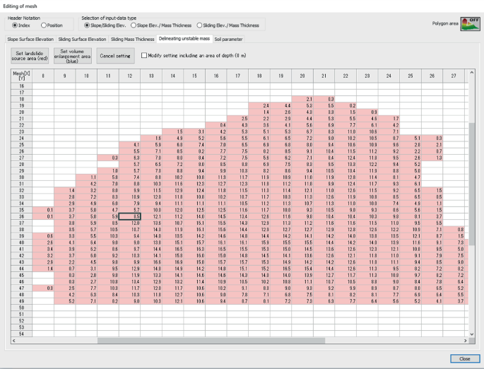

  

  Screenshot of the delineating unstable mass tab of the editing of mesh window

3.5 Fill and Excavate Topography

The sliding surface and original topography of the ground can be created using the fill and excavate options in LS-RAPID. The use of these options will require that the mesh data of the slope surface be inputted. The procedures are provided in the video tutorial titled, “5. Filling and Excavation,” while a brief summary of the steps is provided below:

• 1. To use the fill and excavate options in LS-RAPID, the “Filling and Excavating the Current Topography to Estimate Pre-failure Topography” window will be needed. This window, shown in Fig. 20, can be opened using one of the following three methods:

  Fig. 20

  

  Delineating unstable mass tab in the editing of mesh window

  • a. From the “Edit” menu in Fig. 12, select the “Recover (Source area/Deposition area)” option. Or,

  • b. Click the “Recover (Source area/Deposition area)” icon in the Toolbar. Or,

  • c. From the “Flow” panel, click on the “Editing of mesh” button in Section “1:Mesh” to get the “Editing of mesh” window in Fig. 17. After clicking on the “Creating of sliding surface” button, select, “Create sliding surface section with recovery setting (for previous landslides)” option and click “Ok.”

• 2. Landslides will cause differing changes to the topography that depend on the locations of the source and depositional areas. These zones should be delineated using the options in the “Delineate an area for modifying geographical features” section (Fig. 20). Specifically,

  • a. Source areas will be those that have experienced a reduction in the elevation as a result of the landslide. Therefore, the filling of these areas will be necessary to return to the original ground surface. These areas are defined by selecting the “Recovery of Source area by filling (Yellow)”. The source locations should then be selected in the “Input parameters on the mesh chart (Input depth of mass)” section in the window. Using the “Set for all” button, the selected cells or highlighted region will be set as the source area that needs to be filled to obtain the original ground surface.

  • b. On the other hand, deposition areas will have experienced an increase in the elevation from the landslide and will need to be excavated to reach to the original ground surface. The definition of the depositional area is very similar to the delineation of the source area. The radial button for “Recovery of Deposition area by excavation (Green)” should be selected. The cells for the depositional area should be selected in the “Input parameters on the mesh chart (Input depth of mass)” section. Finally, click on “Set for all” to assign the highlighted cells or section as the deposition area.

  • c. If an error occurs, the “Undo of setting (White)” option can be used. Like the other options, the associated radial button should be selected, the cell/s that needs to be cleared should be selected from the “Input parameters on the mesh chart (Input depth of mass)” section and the “Set for all” button should be clicked.

  • d. The source and deposition areas or removal of these areas can also be selected using a mouse by checking the “Input with a mouse” box in the top left part of the window and then left clicking while pressing down the “Shift” key on the contour map. The “Set for all” button still needs to be clicked once the user is ready to assign the modification to the selected area/s.

• 3. Once the filling and excavation areas have been defined, it will be time to start the recovery of the original ground surface. This will be done through the “Start recovery (Source area/Deposition area)” section in the window. Once the direction of smoothing for the recovery is selected, click on the “Recalculation” button. The changes in the depth of the sliding mass will be tabulated in the “Input parameters on the mesh chart (Input depth of mass)” section once the recalculation is complete.

• 4. Upon completion of the modifications to the topography to obtain the original ground surface, click “Ok (Reflection topographical recovery)” button. This will yield a confirmation message. To confirm that the recovered topography be added to the LS-RAPID model, click “Ok.” Otherwise, click “Cancel.”

  • a. When “Ok” is clicked, the slope surface inputted in LS-RAPID (that is, the slope surface prior to recovery) will be taken as the sliding surface. The new slope surface will be the source area that was created by filling. However, if only excavation was applied to the model, the sliding surface and slope surface will coincide and the original slope surface data will be deleted in these deposition area.

  • b. If “Cancel” is clicked, the confirmation window will disappear and the “Filling and Excavating the Current Topography to Estimate Pre-failure Topography” opened before (Fig. 20) will return.

In the fill regions, the recalculation process finds a standard line that best fits the current slope surface topography. If the elevation of the mesh is less than that of the standard line, the value is increased until the elevation of the mesh is equal to the elevation of the standard line. In the case, when the elevation of the mesh is greater than the elevation of the standard line, the recalculation process will not adjust the elevation. In contract, in excavate regions, the elevation of those regions where the mesh elevation is less than that of the standard line will be increased to the elevation of the standard line. For all other mesh locations, the elevation remains unchanged.

Rather than using the automatic recalculation process described above, it is also possible to fill and excavate the source and deposition areas manually. To do so, the changes in the elevation (or the depth of the mass) should be entered into the “Input parameters on the mesh chart (Input depth of mass)” section in the “Filling and Excavating the Current Topography to Estimate Pre-failure Topography.” If manual inputs are entered, the input data will remain valid (or will be what is used in the computations) until the “Recalculation” button is clicked.

3.6 Determine Source and Enlargement Areas

After the slope and sliding surfaces have been modeled in LS-RAPID, it is possible to visualize the distribution of the unstable mass in the calculation area. Using this information, the landslide source area and the volume enlargement areas can be specified. The procedures to specify these areas are available in the video tutorial titled, “6. Delinating Unstable Mass.” The steps are also summarized below:

• 1. Open the “Editing of mesh” window from Fig. 17. As a reminder, this can be done in one of two different ways: (a) By selecting “Delineation of unstable mass” from the “Edit” menu, or (b) Clicking the “Delineating unstable mass” button in Section “1: Mesh” of the “Flow” Panel (Fig. 9).

• 2. In the “Editing of mesh” window, select the “Delineating unstable mass” tab to get to window in Fig. 21.

  Fig. 21

  

  Delineating unstable mass tab in the editing of mesh window

• 3. The cells corresponding to the source area or the volume enlargement area can now be assigned. To do this, the cells that belong to the source area should be selected and the “Set landslide source area (red)” button should be clicked. Similarly, by selecting the cells corresponding to the volume enlargement areas and clicking the “Set volume enlargement area (blue)” button, the selected cells will be said to belong the volume enlargement area. The color of the cells will change to red if they have been assigned to the source area or blue if they have been assigned to the volume enlargement area. Unassigned cells will remain white.

• 4. If an error is made, the cell/s with errors can be selected and “Cancel setting” button can be clicked to remove the assignment of those cells to either the source area or the volume enlargement area.

• 5. Once the assignments have been made, click the “Set Completed” button.

3.7 Input Soil Properties

Before the soil properties are inputted in to the LS-RAPID simulation, it is important to understand what soil properties will be needed and some of the ways that they can be obtained. Specifically, the following parameters will be needed for simulations in LS-RAPID:

• Lateral pressure ratio,

• Friction coefficient inside landslide mass,

• Friction coefficient during motion at sliding surface,

• Steady state shear resistance at sliding surface,

• Rate of excess pore-pressure generation, and

• Unit weight of mass.

In addition to the above parameters, the peak friction coefficient at sliding surface and the peak cohesion at sliding surface will be needed in simulations that consider strength reduction in full simulations.

The techniques to measure these parameters are provided in many geotechnical engineering textbooks with specific procedures in testing standards such as those by the American Society of Testing and Materials (ASTM). In addition, Tiwari and Ajmera (2018) describes all of the basic laboratory tests in a living document. Therefore, specific details regarding the measurement of these parameters is not provided here.

3.7.1 Typical Ranges

Typical ranges for the different soil properties are provided in this paper. Engineering judgement should be utilized if parameters are selected from the typical ranges provided here. Furthermore, it is noted that the information presented here is not a substitute for high quality sampling and testing, which, when appropriately applied, provides the best estimations of the field conditions.

Some typical values for the soil properties are summarized below:

• Lateral pressure ratio: 0.30–0.50

• Friction coefficient inside landslide mass: 0.36–0.58

• Friction coefficient during motion at sliding surface: 0.46–0.70

• Steady state shear resistance at sliding surface: 5–50 kPa

• Peak friction coefficient at sliding surface: 0.65–0.78

• Peak cohesion at sliding surface: 10–100 kPa.

The rate of excess pore pressure generation will have a value between 0 and 1.

3.7.2 Correlations

There are a number of correlations available in the literature to estimate the residual shear strengths of soils. Some of the available relationships at the time of publication are summarized in this section. More details are available in Tiwari and Ajmera (2020). Table 3 presents a summary of correlations for the residual shear strength available in the literature. Several relevant relationships are provided in Figs. 22, 23 and 24.

Table 3 Summary of available residual shear strength correlations

Fig. 22

Relationship from Tiwari and Marui (2003) for the residual friction angle in terms of the liquid limit and clay mineralogy

Fig. 23

Relationship from Tiwari and Marui (2003) for the residual friction angle in terms of the plasticity index and the clay mineralogy

Fig. 24

Triangular correlation chart for clay mineralogy to estimate the residual friction angle developed by Tiwari and Marui (2003)

3.7.3 Inputting Soil Properties in LS-RAPID

The procedures for inputting the soil properties in the LS-RAPID simulation are summarized below:

• 1. In the “Flow” panel, click on the “Soil parameters” button from Section “2: Calculation condition.” This section is shown in Fig. 25. The “Editing of Mesh” window from Fig. 17 will be displayed.

  Fig. 25

  

  Screenshot of section 2: calculation condition of the flow panel

• 2. In the “Editing of Mesh” window, select the “Soil parameter” tab, as shown in Fig. 25.

• 3. The values of the parameter being edited should be entered. This can be done manually by entering the data corresponding to the x- and y-coordinates shown in the table if the “Position” radial button in selected under “Header” or to the x- and y- mesh indices if the “Index” radial button is selected. Alternatively, a specific value can added to several selected cells using the “Set in selected rectangle” button.

• 4. These steps should be repeated until the values of eight different parameters are entered in the “SoilParameter” tab. These parameters are: (1) lateral pressure ratio, (2) friction coefficient inside landslide mass, (3) friction coefficient during motion at sliding surface, (4) steady state shear resistance at sliding surface, (5) rate of excess pore pressure generation, (6) peak friction coefficient at sliding surface, (7) peak cohesion at sliding surface, and (8) unit weight of mass. A description of the soil parameters can be obtained in LS-RAPID by clicking the “About parameters of soil characteristics” button. It is noted that except parameters 6 and 7 (peak friction angle and cohesion at sliding surface), all of the other parameters are required for the simulation. The parameter that is being edited will be indicted in the “Editing of Mesh” window with an asterisk (*) in the “Edit” column of the table. For example, in Fig. 26, the lateral pressure ratio is being edited.

  Fig. 26

  

  Soil parameter tab in the editing of mesh window

The procedures for inputting soil properties are also illustrated in the video tutorial titled, “7. Soil Parameters.”

3.8 Simulation Conditions

There are several different modes to simulate landslides in LS-RAPID. The procedures for performing these simulations are described below:

• 1. Open the “Set condition for calculation (Landslide)” window shown in Fig. 27 by clicking the “Conditions for calculation” button from Section “2:Calculation condition” in the “Flow” Panel on the left side of the program.

• 2. The type of simulation that will be performed is selected from the “Condition of simulation” section in the “Set condition for calculation (Landslide)” window.

  • a. If only the motion needs to be determined, the “Motion simulation” radial button should selected from the “Motion simulation” subsection.

  • b. Otherwise, a full mode simulation will need to be selected from the “Fullmode simulation (Initiation + Motion + Expansion)” subsection. Three radial buttons present the options available for the simulation type, namely, normal simulation, seismic simulation and rainfall simulation. Depending on the radial button selected, different options and parameter requirements will be made available on the “Set condition for calculation (Landslide)” window shown in Fig. 27.

    Fig. 27

    

    Set condition for calculation (landslide) window

    • i. Selection of the “Normal simulation” or “Seismic simulation” radial buttons will make available a check box for “With pore pressure.” This option allows pore water pressure to be considered as the trigger for the landslide. To use this option, rainfall data will be necessary.

    • ii. Details of normal and rainfall simulations procedures are provided in the video tutorial titled, “8. Setting for Rainfall Induced Landslide,” whereas, the seismic simulation procedures are in the video tutorial titled, “9. Settings for Earthquake Induced Landslide.”

• 3. To perform a normal simulation with pore pressure, the following steps will need to be followed:

  • a. In the “Method to give a graph of pore pressure ratio (ru)” section shown in Fig. 27, enter the time at which the rainfall begins in the “Time to start” box.

  • b. The pore water pressure condition will then need to be specified by selecting either the “Static” or “Survey” radial buttons.

    • i. If the “Static” radial button is selected, the pore pressure ratio will remain constant at the “Ru” value specified for the “Duration” provided in the data entry boxes.

    • ii. Selection of the “Static” radial button will also provide an option to fluctuate the pore pressure value by checking the “Fluctuate a value” box. Checking this box will yield four locations requiring parameters. The user should enter the minimum pore pressure ratio in the “Min” box and the maximum value that the pore pressure ratio reaches in the “Max” box. The time required to reach this maximum pore pressure ratio should be entered in the “Max Time” box. In other words, at the start of the rainfall simulation, the pore pressure ratio will then begin at the value entered in the “Min” increasing to the value in the “Max” box over the duration noted in the “Max Time” box. This maximum value will then remain constant for the duration provided in the “Duration” data entry box.

    • iii. If the “Survey” radial button is selected, the rainfall will vary according to the pore pressure ratios provided at different time intervals. This pore pressure ratio as a function of time is specified by clicking the “Edition of ru” button, which will yield the “Pore pressure ratio” window shown in Fig. 28.

    • iv. The “Pore pressure ratio” will also contain a table in which the pore pressure ratios should be entered at different times of the rainfall event being simulated.

    • v. Once the rainfall data has been entered, Click “Ok” to return back to the “Set condition for simulation (Landslide)” window in Fig. 27.

    • vi. Visualization of the rainfall data can be obtained by clicking the “Graph preview” button in the bottom left corner of the Set condition for calculation (Landslide)” window in Fig. 27.

• 4. A rainfall simulation can be performed by selecting the “Rainfall simulation” radial button. The associated steps for this simulation are:

  • a. Click on the “Edition of rainfall” button to open the “Rainfall Data” window shown in Fig. 29.

    Fig. 28

    

    Pore pressure ratio window obtained by clicking the edition of ru button in the set condition for calculation (landslide) window

  • b. The ten-minute rainfall intensities should be entered at different times of the rainfall event being simulated in the window in Fig. 29.

    Fig. 29

    

    Rainfall Data Window Opened when Edition of Rainfall Button in Clicked

  • c. Once the data has been entered, click “Ok.”

  • d. As before, visualization of the rainfall data can be obtained by clicking the “Graph preview” button in the bottom left corner of the Set condition for calculation (Landslide)” window in Fig. 27.

• 5. Procedures associated with the seismic simulations are described below. Note that the seismic waveforms can be visualized by clicking the “Graph preview” button in the bottom left corner of the Set condition for calculation (Landslide)” window in Fig. 27.

  • a. If pore pressure is also considered as part of the triggering mechanism, the “With pore pressure” box should be checked. This will require information to be entered into the “Method to give a graph of the pore pressure ratio (ru) section.” The procedures for this entering the relevant information for this triggering mechanism have been explained in Step 3.

  • b. The “Method to give a graph of seismic coefficient” section of the “Set condition for calculation (Landslide)” window will allow the user to input data related to the seismic excitation at the landslide location. The beginning of the seismic load will correspond to the time entered in the “Time to start” box.

  • c. The user then has three options to apply the cyclic loads. These are given by the radial buttons labeled, “Static,” “Cyclic,” and “Seismic.” The options selected will determine whether the cyclic loads remain constant or fluctuate with time. Specifically, when “Static” is selected, the seismic coefficient will experience a linear variation with time. Data corresponding to the seismic coefficients should be entered into the “Static/Cyclic parameter setting” subsection. The selection of “Cyclic” will cause the seismic coefficient to fluctuate following a sine waveform. Furthermore, the amplitude of the seismic coefficient will experience a linear change. Finally, seismic wave form data from an actual ground motion may be entered into the simulation when the “Seismic” option is selected. Thus, the seismic coefficient will vary based on the data inputted into the program.

• a. For the “Static” option,

  • i. Horizontal seismic coefficients will be entered by checking the “Horizontal seismic coefficient (Kh)” box. This coefficient can be entered in one of two ways: (1) Directional coefficients corresponding to the x- and y-directions can be entered in the boxes for the “X-direction coefficient Kx” and the “Y-direction coefficient Ky,” respectively, when the “Direction coefficient” radial button is selected, or (2) The horizontal coefficient can be entered directly by clicking the “Horizontal coefficient” radial button. In this option, the value of the horizontal coefficient and the corresponding seismic direction should be entered into the “Kh” and “Seismic direction θs” boxes, respectively.

  • ii. If a vertical seismic coefficient is needed, the “Vertical seismic coefficient (Kv)” box should be checked and the corresponding seismic coefficient should be entered into the data box.

  • iii. Clicking the “Substitute the direction of landslide profile” will cause the direction of the longitudinal landslide section to be set as the direction of the seismic coefficient if an ellipsoidal sliding surface was created.

  • iv. In the “Frequency/MaxTime/Duration” subsection, enter the “Duration” of the seismic load.

  • v. If the “Fluctuate a value” box is checked in the “Frequency/MaxTime/Duration” subsection of Fig. 27, the static seismic coefficient will begin at zero and linearly increase to the values of the seismic coefficients over the time specified in the “Max Time” box. The seismic coefficient will then remain constant before linearly decreasing from the maximum value to zero over the same “Max Time” duration. The total duration of the seismic load including the linear increase at the start and the linear decrease at the end will still correspond to the “Duration” value provided.

• b. For the “Cyclic” option,

  • i. Follow the steps in given in Step 5.d.i to 5.d.iii.

  • ii. In the “Frequency/ MaxTime/ Duration” subsection, the frequency of the sinusoidal waveform should be entered in the “Hz” box and the number of cycles of loading in the “Total Cycle (N)” box.

  • iii. Checking the “Fluctuate a value” box will yield some additional options. Specifically, the number of cycles required to reach the maximum seismic coefficient should be entered in the “Kmax Cycle (N)” box. This will indicate the number of cycles over which the amplitude of the sine wave is increased to the maximum value specified. This increase will occur in a linear fashion. It also corresponds to the number of cycles at the end of the seismic waveform over which the maximum seismic coefficient is decreased to zero.

• c. For the “Seismic” option,

  • i. Seismic coefficient data is entered by clicking on the “Edition of seismic waveform” button. This will open the “Data registration of seismic waveform” window. Figure 30 contains a screenshot of this window.

    Fig. 30

    

    Data registration of seismic waveform window screenshot

  • ii. A name for the waveform should be entered in the text box just beneath the text, “Case 1 Seismic Waveform.”

  • iii. In the table just beneath the name, the user should enter the time and corresponding values of the acceleration for the east-west, north-south and up-down directions. This information should inputted into the corresponding columns titled, “Time,” “EW-Acc,” “NS-Acc,” and “UD-Acc,” respectively. When entering the data, the time must be entered in chronological order with the corresponding acceleration values in the associated row.

  • iv. Up to three different seismic waveforms may be entered into the program. The steps for entering the data are the same, except the data will be entered to correspond to the seismic waveform case as shown in Fig. 30.

  • v. Once the seismic wave form data has been entered, click “Ok” to return to the “Set condition for calculation (Landslide)” window from Fig. 27.

  • vi. In the “Seismic parameter setting” subsection, the maximum seismic coefficients in the x-, y-, and vertical directions will be displayed in the “Kx max,” Ky max,” and Kv max” boxes, respectively. The amplitude of these waveforms can be scaled using the factors entered in the “EW Acc (gal)/980x,” “NS Acc (gal)/980x,” and “UD Acc (gal)/980x,” boxes, respectively.

• 6. Once the required data for the simulation have been entered using the procedures described above, the next section that will require user input will be the “Parameters for condition for strength reduction” in the “Set condition for calculation (Landslide)” window in Fig. 27. In the full mode simulations, the peak values of the friction coefficient and the cohesion are reduced to the normal motion values in the unstable mass. In other words, tan φ_p and c_p will reduce to tan φ_m and c_m, respectively.

  • a. The reduction in the friction coefficient and the cohesion will commence when the travel length of the landslide reaches the distance specified in the “From (DL)” box and continue until the distance specified in the “To (DU)” box. Once the travel length exceeds the value in the “To (DU)” box, normal simulation will begin.

  • b. In the “Except source area (by depth of mass)” box, the user should specify the depth of the sliding mass (Δh_cr), which when reached will also trigger the start of the normal motion simulation signifying the completion of the reduction of the friction coefficient and cohesion.

    • i. Buoyancy can be incorporated into the simulation by checking the “Calculate submergence” in the “Setting of the submergence calculation” section. Doing so will allow the user to enter the depth of the ground water table (or the interface between the submerged and unsubmerged soil) in the box for the “Level of the water surface.” The “unit weight of water (γ w)” box should be used to specific the unit weight of water or the weight of water in a unit volume.

• 7. Once all of the simulation information has been entered, click the “Set Parameters” button in the bottom right corner of the “Set condition for calculation (Landslide)” window in Fig. 27.

• 8. The “Graph Preview” button in the bottom left corner of “Set condition for calculation (Landslide)” window will allow the user to view the ground motion that will be applied in the simulation based on the parameters entered in the steps described above.

3.9 Setting Time Steps

The degree by which the motion proceeds in the simulation can be adjusted by using a time step. The video tutorial titled, “10. Setting Time Step,” explains the procedure, which is also summarized below:

• 1. Open the “Setting time step” window presented in Fig. 31. This window can be obtained through the “Flow” panel on the left side of the LS-RAPID program. Under Section “2: Calculation condition,” click on the “Setting time step” button.

  Fig. 31

  

  Setting time step window

• 2. The time step can be set to remain constant throughout the simulation by checking the “Calculate with a definite time step in the whole process” box. Otherwise, the parameters in the “Set general time step” section should be edited.

• 3. The time step for the first step in the simulation should be specified in the “Initial time step (DT1)” box.

• 4. The next time step will be calculated from the average maximum velocity. In the event that this time step exceeds the value in the box labeled, “Upper bound value of time step,” the next time step will be value provided in this box.

• 5. The number of calculations per mesh at which the next time step should be calculated should be provided in the next box.

• 6. In the subsection titled, “Time step for simulating initiation process,” the time step used in the initial simulation will be terminated as the reduction in the shear resistance will be complete. After reaching this distance, the simulation will use the time step corresponding to the motion simulation.

3.9.1 Setting of Other Conditions

There are several simulation settings that are not used very frequently. This section will quickly summarize those settings. To obtain these settings, click on the “Setting other conditions” button from Section “2: Calculation condition” in the “Flow” panel. The “Setting other conditions” window, displayed in Fig. 32, will open. The video tutorial describing these additional conditions is titled, “11. Setting Other Conditions.”

Fig. 32

Setting other conditions window screenshot

3.9.2 Non-frictional Energy Consumption

Checking the “Trigger non-frictional energy loss function” in the “Non-frictional energy consumption” section will cause this energy consumption to be considered in the simulation. It will be necessary to specify the coefficient, α, at which the non-frictional energy function is triggered. Two additional options also exist in this section, which allow the non-frictional energy loss function to be triggered when the specified velocity or specified depth of mass is reached, when the corresponding boxes are checked.

3.9.3 Other Settings

Under the “Set for” subsection, several other setting options are present. These are as summarized below:

• The “Threshold of flow rate (neglected below this value)” setting allows the user to specify the minimum amount of soil in the calculated mesh that is moving within a unit of time. When the flow is less than the value specified, the mesh rejects the flow. This value will depend on the size of the landslide, but a good initial estimate is 0.01 m³/sec.

• Landslide movements down a torrent will be concentrated along the torrent. However, some of the upper part of the landslide may cross over the ridge when it is higher than the ridge. Checking the “Calculate the case of crossing over a ridge” option will consider this effect.

• Increases in the lateral pressure are expected when the vertical stress increases. These increases depend on the lateral earth pressure coefficient. When the “Calculate increased lateral pressure at vertical earthquake loading” box is checked, this effect will be considered in the simulation.

• A cohesion value can be assigned to all of the geographical features of the landslide mass with the use of the “Cohesion inside mass” data box. Similarly, the cohesion along the entire sliding surface during landslide motion can be assigned using the “Cohesion at sliding surface during motion” box.

• During the simulation, the total volume of the soil mass should not change. However, in unsteady conditions, this volume may increase and the effect can be adjusted by increasing the velocity by a certain percentage before the simulation begins in the “Calibration parameter of calculated landslide mass” subsection.

3.9.4 Output Settings

The settings associated with the outputs from the simulation should be configured next. The following steps will describe how this configurations can be applied in LS-RAPID. Users may also refer to the video tutorial, titled “13. Output Setting for Landslide Simulation.” These settings can be accessed through the “Flow” Panel in Section “3: Simulation” by clicking the “Set calculation output” button. The “Output setting” window pictured in Fig. 33 will open. The options available in each section of this window will be discussed in this section.

Fig. 33

Output setting window screenshot

3.9.5 Calculation Step Numbers (for Result Saving)

In the “Calculation step numbers (for result saving)” section of the “Output setting” window in Fig. 33, the value entered in the “Maximum step” data box will indicate the number of steps after which the results are drawn in the topographical display in LS-RAPID and when the results are saved. The “Drawing interval” represents the time (or step) interval at which the geographical features are updated during the simulation. Additionally, it also indicates the interval at which intermediate simulation results are saved.

The maximum x- and y- velocities will be obtained as an average of the corresponding results at a number of sample locations in each mesh. The number of samples that should be used for this average can be specified in the box labeled, “Necessary number of samplings to display Umax, Vmax” in the “Calculation step numbers (for result saving)” section.

The LS-RAPID simulation terminates when all solid features have stopped moving. A user may specify that the simulation continue beyond this point by specifying the “Minimum time for simulation.” This will cause the simulation to continue to run even after the all the solid features have stopped until the time entered is reached.

3.9.6 Output of Altitude Information

The “Output of altitude simulation” section primarily contains the settings to save output files. Specifically, when the “Output the altitude calculation result data” box is checked, elevation data after the simulation will be saved into the same folder as the project file. If a different location is desired, the user may specify the preferred location by using the open folder icon in the “Folder for output files” subsection. This location can be removed from the simulation by clicking the delete folder icon.

The three-dimensional view in the LS-RAPID display panel will not be updated when the “No refresh view during calculation” box is checked. It is should be noted that the computations will be performed faster if the display does not need to be periodically updated during the simulation process. Settings associated with the display during the simulation are set in the “Drawing” section of the “Output setting” window in Fig. 33. Details regarding these settings are provided next.

3.9.7 Drawing

During the simulation, the calculation time can be displayed in either seconds or hours by selecting the radial button next to “How to display calculation time” in the “Drawing” section. Any comments that should be displayed during the simulation should be provided in the text box under the “Comments field.”

When drawings are being periodically generated during the simulation, the “Waiting time for drawing result data” will indicate the time at which the output files for the altitude will be read and displayed. In the display, it may be of value to display the seismic and/or rainfall functions as the simulation progress. The length of the horizontal (or time) axis for these landslide triggers can be specified in the “Drawing period of landslide trigger” data box.

3.9.8 Output Options

The last section in the “Output settings” window shown in Fig. 33 is “Output settings.” Under the “Assign the head words for output files,” the word(s) that will proceed the names for all files and folders generated during the simulation can be specified. This is done by clicking the open folder icon and selecting the location at which the output files will be stored and typing the word(s) that should be used as a prefix in all of the output files and folders. It is noted that by default, the location shown in the window that opens when the open folder icon is clicked corresponds to the location specified in the “Folder for output files” entry in the “Output of altitude information” section. These word(s) that serve as a prefix to the file and folder names can be deleted by clicking the delete folder icon.

By default, all of the data from the beginning of the simulation will be exported and saved. However, the user may also specify the range of steps across which the data should be saved if all of the data is not necessary. This can be done by entering the desired range values in the data boxes in “Step range to output calculation range.”

The text files that will be generated in the simulation can be formatted in the “<Text files>” subsection. Users have the choice between the use “Space” or “Comma” delimiters between data in the text files. The “Output Digit” will specify the number of decimal places that are provided for the depth of the soil mass in the text files, while “Output form” indicates how these data will be displayed. In particular, if “Matrix” is selected, the output data will be formatted in a matrix, whereas, the selection of “Control point form” will format the text files to have rows containing the mesh ID and the depth of soil mass.

The data that can be exported in the output files during the simulation can be selected from the check boxes at the bottom of the “<Text files>” subsection. When “‘VALUE’” is selected, the depth of the unstable soil mass for each mesh will be saved, while “’GRAPH’” will display the depth of the unstable mass for each mesh graphically. The velocity of the soil mass can be outputted by checking the “’U’,” “’V’,” and/or “’UV Bar’” boxes. U and V represent the velocities in the x- and y-directions, respectively. The mean value of the velocity will be given by UV option.

The images generated during the simulation can be formatted using the options in the “<Picture files>” subsection. Images can be saved as “’JPEG’ Files” and/or “’AVI’ File” by checking the appropriate box(es). The number of images to be saved per second of the simulation should be specified in the box for “(frames/sec).” The area that will be included in the images is specified by the settings in the “Picture clipping area” subsection. Selection of “Application area” will focus on images associated with the regions with movement in a two-dimension plan view of the failure. By contrast, the selection of “3D-View area” will result in images containing three-dimension views of the simulation area based on the display in the viewing panel in the LS-RAPID program.

3.9.9 Background Images in Simulation

Users may find it valuable to have an image of the topography from Google Earth or other sources as the background for the simulation area. Steps to insert and display this image can be found in the “12. Setting Background Image for Topography” video tutorial. Additionally, the steps are briefly summarized in this section.

• 1. As shown in Fig. 34, select “Setting background image file (R)” from the “File(F)” menu. This will open in the “Setting background image file” window shown in Fig. 35.

  Fig. 34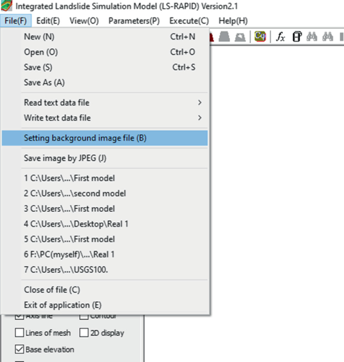

  

  Screenshot of file menu in LS-RAPID

  Fig. 35

  

  Setting background image file window

• 2. Use the “Select File” button from the “Background image file” section to navigate to the location and select the file associated with the background image. Please note that only BMP and JPEG files can be used for this setting. Once the file has been selected, click the button labeled, “Open.”

• 3. The selected image will be displayed in the “(Image Preview)” section in the “Setting background image file” window shown in Fig. 35.

• 4. In the “Coordinate relation” section, specify the coordinates of the corners of the images. The labeling of these corners is identified in the “(Relation with simulation area)” section.

  Specifically, “Pos. A” refers to the bottom left corner of the images while “Pos. B” is the bottom right corner. Similarly, “Pos. C” and “Pos. D” correspond to the top right and top left corners, respectively. The x-coordinate should be entered in the cells under the “PX” column heading, whereas, the y-coordinates should to be entered in the “PY” column.

• 5. Click “Ok.” This will result in the background of the topography being replaced by the image selected based on the coordinates provided.

3.9.10 Starting a Simulation and Displaying the Results

To begin the simulation, the user should click on the “Start simulation” button in Section “3: Simulation” of the “Flow” panel. Users may also refer to the video tutorial, titled “14. Start Simulation.” This will result in a notification, like that shown in Fig. 36, asking the user to confirm that the simulation should be started. When “Ok” is clicked, the simulation will begin. The pause, play and stop icons in the toolbar can used to temporarily pause, restart and stop the simulation, respectively.

Fig. 36

Notification confirming the start of simulation when start simulation button is clicked

There are several options that can be used during the simulation. Clicking the black binoculars icon in the toolbar will open the “Mesh value monitor” window, similar to that pictured in Fig. 37. This window will display the mesh ID and associated values of various different parameters at the time step corresponding to when the black binoculars icon was clicked. The drop down menu at the top of this window will allow the user to select which of the various parameters used and/or generated at that specific time step should be displayed. Specifically, the following nine options are available: (1) friction coefficient at sliding surface, (2) cohesion at sliding surface, (3) present mass distribution, (4) velocity along x-axis, (5) velocity along y-axis, (6) flow rate along x-axis, (7) flow rate along y-axis, (8) accumulated mass displacement, and (9) maximum velocity record.

Fig. 37

Mesh value monitor window opened by black binocular icon

The green binoculars icon can be used to display the triggering factors in the simulation. Figure 38 contains the “Monitor value” window that is opened when the green binoculars icon is clicked. In this window, both the rainfall and earthquake loading information will be displayed.

Fig. 38

Monitor value window opened by green binoculars icon

Upon the completion of the simulation, the simulation results can be displayed using the “Result of simulation” button. This button is located in Section “3: Simulation” in the Flow panel.

4 Examples and Tutorials

4.1 Generated Simple Slope with an Ellipsoidal Sliding Surface

Interested users may also follow a video tutorial with this example, titled, “15. Rainfall-Induced Simple Slope Landslide Tutorial.”

4.1.1 Initial Topography

4.1.1.1 Simulation Area

To create a simulation area within LS-RAPID for a simple slope, click on the “Simulation area” button in the Section “1: Mesh” within the “Flow” panel located on the left side of the program. This will result in the image in Fig. 9.

In the “Setting of simulation area and input-data type”, input values of the x- and y-coordinates, as indicated in Fig. 9. The simulation area will be 350 m in x-direction and 440 m in y-direction. The pitches for x- and y-directions are set as 10 m each in the second component of “Mesh setting of simulation area.” The numbers of grids are automatically calculated based on the inputted values of x- and y- coordinates and pitches. The simulation area is illustrated in the bottom part of the window. Click “OK” to complete setting of simulation area.

4.1.1.2 Editing Mesh

The second step is to establish the topography of the simple slope. In this example, the mesh data for the topography of the slope is estimated in an Excel file (as shown in Fig. 39) and then is inputted into LS-RAPID. Mesh data is added into the calculation area using “Editing of mesh” button of the Section “1: Mesh” in the “Flow” panel (Fig. 9).

In the “Editing of mesh” window, select the “Index” option for the “Header Notation” section, select “Slope Elev./Mass Thickness” option in the “Selection of input-data type” section. In this case, the mesh is represented with the numbers associated with the grid lines in the calculation area and the slope surface elevation and the sliding mass thickness will be defined.

Fig. 39

Cross section of the simple slope

Topography data is inputted into the “Slope Surface Elevation” tab by copy-pasting from the Excel file. This step is illustrated in Fig. 40. The topography mesh of the simple slope will then be displayed in the viewing panel as shown in Fig. 41.

Fig. 40

Input topography mesh data into the calculation area using “editing of mesh”

Fig. 41

Topography mesh of the simple slope example

4.1.2 Creating Sliding Surface

The potential sliding surface is created using ellipsoidal parameters. As described previously in Sect. 3.4.1, the user can use one of the three different ways to begin creating the ellipsoidal sliding surface.

In this example, the longitudinal section is defined by inputting start (180, 450) and end (180, 150) points in the “Selection longitudinal section” table. The locations of passing points A, B, and the center of ellipsoid on the longitudinal section of the sliding surface are selected as (35, 110), (165, 50), and (200, 160), respectively. The locations of passing points C and the center of ellipsoid on the crossing section are (120, 95), (180, 160), respectively. The location of passing point D is automatically calculated. The parameters used in this example for this paper are shown in the screenshot in Fig. 42.

Fig. 42

Select profile to draw ellipsoidal sliding surface for the simple slope

4.1.3 Delineating Unstable Mass

The delineating unstable mass step is used to specify the landslide source and enlargement areas. In Section “1: Mesh” of the “Flow” panel (Fig. 9), click the “Delineating unstable mass” button. Select all the cells corresponding to the source area and then click “Set landslide source area (red).” The color of the cells should change to red. The depth of unstable mass in the enlargement area is set to 5 m. Select the cells corresponding to the volume enlargement areas and click the “Set volume enlargement area (blue)” button. The color of the cells of the volume enlargement area will become blue. This is illustrated in Fig. 43.

Fig. 43

Assignment of source and volume enlargement areas of the simple slope landslide example

4.1.4 Input Soil Properties

In Section “2: Calculation condition” of the “Flow” panel, click on the “Soil parameter” button to input soil properties. Values of the parameters for this example are selected as approximately the average of the typical values suggested in the program and are specified in Table 4. Figure 44 shows the lateral earth pressures entered in the model.

Table 4 Soil parameter used in the simulation of the simple slope landslide

4.1.5 Simulation of a Rainfall-Induced Landslide on Simple Slope

First, a rainfall-induced landslide simulation is performed on the geometry of the simple slope described previously in this chapter. The triggering factor of the landslide is considered to be a high-intensity or/and long-term rainfall, which causes a rise in level of the groundwater table. This will subsequently cause an increase in the pore water pressure and an associated decrease in the shear strength on the sliding surface. The heavy rainfall used in the simulation occurred from 14 to 18 May 2016 which triggered the Aranayake catastrophic landslide in Sri Lanka (Dang et al. 2019). The observed rainfall data associated with this event is provided in Table 5. From the observed rainfall, the water pressure ratio (r_u) was calculated using a SLIDE model (Liao et al. 2010). The simulation is set to 80 h corresponding to the more than three days of the rainfall event.

Table 5 Data of Aranayake rainfall and pore pressure ratios used in the simulation

Fig. 44

Setting soil parameters (lateral pressure ratios) for the simple slope example

4.1.5.1 Setting Simulation Conditions

In LS-RAPID, click on the “Conditions for calculation” button from Section “2: Calculation condition” in the “Flow” Panel to open the “Set condition for calculation (Landslide)” window. Figure 45 shows the window that will be open when these steps are followed.

Fig. 45

Set conditions for rainfall-induced landslide simulation

Select the “Rainfall simulation” radial button to conduct a rainfall-induced landslide simulation. Click on the “Edition of rainfall” button to input the rainfall intensities (Fig. 46). For the “Method to give a graph of pore pressure ratio (ru),” select the “Survey” radial button and click on the “Edition of ru” button to input the pore pressure ratio data in the “Pore pressure ratio” window, as shown in Fig. 47. To reduce the computation time for the landslide simulation, the “Calculation pitch” and the “Velocity limit” are set as 36,000 times and 0.10 m/s, respectively. The pore pressure ratios estimated in Table 5 are entered into the “Pore pressure ratio” window. Once the rainfall and pore pressure ratio data have been entered, their graphs can be previewed, as shown in Fig. 48. Click the “Set Parameters” button in the bottom right corner of the “Set condition for calculation (Landslide)” window (Fig. 45) to complete this step.

Fig. 46

“Rainfall data” window with data from Aranayake rainfall provided in Table 5

Fig. 47

“Pore pressure ratio” window with pore pressure ratio data from simple slope example

Fig. 48

(Bottom) Rainfall and (top) pore pressure ratio used as triggering factor for rainfall-induced landslide simulation

4.1.5.2 Setting Time Steps and Other Conditions

For the example simple slope simulation, time steps and other conditions are set as illustrated in Figs. 49 and 50.

Fig. 49

Screenshot of setting time step window

Fig. 50

Screenshot of setting other conditions window for rainfall-induced landslide simulation

Fig. 51

Output settings for rainfall-induced landslide on the simple slope

4.1.5.3 Output Settings

The simulation of the rainfall-induced simple slope landslide described in this section is long (80 h). The output settings selected for this example are shown in Fig. 51. The “Maximum step” is set to 20,000, the “Minimum time for simulation” and the “Drawing period of landslide trigger” are set to 57 h and 10 steps, respectively. The calculation time is set to display in hours. Other items were kept as default values.

Fig. 52

Results of the simulation of the rainfall-induced landslide on the simple slope at a 7 h 30 m 00 s, b 58 h 30 m 00 s, c 68 h 15 m 08 s, and d 68 h 15 m 42 s from the start of rainfall

4.1.5.4 Starting the Simulation and Displaying the Results

The results of the simulation of the rainfall-induced landslide on the simple slope are shown on Fig. 52. The cyan line represents the landslide mass in the source area, while the pink line shows the calculated sliding mass distribution area. When the pore pressure ratio reaches 0.36 at 58 h 30 m 00 s, the failure initiates from the middle of the landslide source area. When the pore pressure ratio reaches 0.42 at 68 h 15 m 08 s, the entire landslide mass has formed and starts to move down at a speed of 20.6 m/s. At 68 h 15 m 42 s, the landslide mass has stopped moving and is completely deposited.

4.1.6 Simulation of an Earthquake-Induced Landslide on the Simple Slope

The second example is to simulate an earthquake-induced landslide on the designed simple slope. Since the slope geometry is the same as the rainfall-induced landslide simulation discussed previously, the steps associated with the creation of the geometry, entering soil properties, and other parameters are not described again. The reader is referred to previous sections in Sect. 4.

The 2008 Iwate-Miyagi earthquake record (MYG004), which triggered the Aratozawa landslides (Sassa 2014a; b) is used as the triggering factor for this example. The earthquake record is illustrated in Fig. 53.

Fig. 53

2008 Iwate-Miyagi earthquake record (MYG004) used as the triggering seismic parameter

A tutorial of the steps involved in preforming this simulation is also included with this paper. This video tutorial is titled, “16. Earthquake-Induced Simple Slope Landslide Tutorial.” Interested users may opt to follow the steps in that video in lieu of the instructions provided below.

4.1.6.1 Setting Simulation Conditions

In LS-RAPID, click on the “Conditions for calculation” button from Section “2: Calculation condition” in the “Flow” Panel. This will open the “Set condition for calculation (Landslide)” window. A screenshot of this window was provided in Fig. 45.

Select the “Seismic simulation” radial button in the “Fullmode simulation (Initiation + Motion + Expansion)” section to conduct the earthquake-induced landslide simulation on the simple slope geometry, as shown in Fig. 54. In this example, pore pressure is not considered as part of the triggering mechanism. Click on the “Edition of seismic waveform” button in the “Method to give a graph of seismic coefficient” section to input the seismic data including name, time and corresponding values of the acceleration for three directions, as illustrated in Fig. 55. In the “Seismic parameter setting” subsection (Fig. 54), the maximum seismic coefficients in the x-, y-, and vertical directions are kept the same as the values in the 2008 Iwate-Miyagi earthquake record (Fig. 53).

Fig. 54

Set conditions for earthquake-induced landslide simulation

Fig. 55

Seismic data of the 2008 Iwate-Miyagi earthquake as Inputted into the “data registration of seismic waveform” window

Once the seismic parameters for the simulation have been entered, their graphs can be previewed as shown in Fig. 56. Click the “Set Parameters” button in the bottom right corner of the “Set condition for calculation (Landslide)” window (Fig. 54) to complete this step.

Fig. 56

Graph of seismic coefficient used as the triggering factor for earthquake-induced landslide simulation

4.1.6.2 Setting Time Steps and Other Conditions

The time steps and other conditions of the earthquake-induced landslide simulation are set similar to the case of the rainfall-induced landslide simulation described earlier in this chapter. The values in this simulation can be found in Figs. 49 and 50.

4.1.6.3 Output Settings

Since the duration of the seismic waveform is about 300 s and the main shock occurs around 10 s, the output settings are selected to clearly show and cover the entire simulation process. As shown in Fig. 57, the “Maximum step” is set to 20,000, the “Drawing interval” is 0.1 s, and the “Minimum time for simulation” is 300 s. The “Drawing period of landslide trigger” is set to 10 s, which corresponds to the period of the main shock. The calculation time is select to display in seconds. All other items are kept at their default values.

Fig. 57

Output settings for earthquake-induced landslide on the simple slope

4.1.6.4 Starting the Simulation and Displaying the Results

The results from the simulation of the earthquake-induced landslide on the simple slope are shown in Fig. 58. When the main shock of the earthquake strikes the slope at 4.3 s, failure initiates in the middle part of the source area. At 11.3 s, the entire landslide mass has formed and begins moving downward at a velocity of 12.7 m/s during the earthquake shaking. At 56.4 s, the landslide mass has stopped moving. As before, in Fig. 58, the cyan line represents the landslide mass in the source area, while the red line shows the area of sliding mass distribution.

Fig. 58

Simulation results for earthquake-induced landslide on the simple slope at a 0.4 s, b 4.3 s, c 11.3 s, and d 56.4 s from the start of earthquake

4.2 Application of LS-RAPID to Rain-Induced Landslides: A Case Study of Atami Debris Flow

From 1 to 3 July 2021, extreme rainfall occurred in the Atami District, Shizuoka Prefecture, Japan causing a catastrophic debris flow on 3 July 2021. A geological map with the debris flow is shown in Fig. 59. The Atami debris flow claimed 27 lives with one missing, three injuries and destroyed 54 houses, as of 10 February 2022 (Shizuoka Prefecture 2022). On 17 January 2022, International Consortium on Landslides (ICL) researchers investigated the landslide area. A sample was taken from immediately behind the exposed scar as shown in Fig. 59 and sent to the Kyoto ICL-SATREPS office for ring shear tests. As shown in Fig. 59, the underlying geology of the source area is andesite to basaltic andesite lava and pyroclastic deposits, which are products of Hakone Volcano (Oikawa and Ishizuka 2011).

Fig. 59

Geological map of study area (this map is made based on the data from the geological survey of Japan and the geospatial information authority of Japan)

4.2.1 Ring-Shear Simulator

Speed control test is used as a basic soil test to obtain soil parameters. In undrained speed control tests, normal and shear stresses in the steady-state condition can be obtained as the mobilized and peak friction angles.

Slow shear speeds should be used in the tests on the fine-grained materials that have low coefficients of permeability and generate pore pressures slowly. The normal and shear stresses acting on the potential sliding surface were reproduced in the shear box. An undrained speed control test was conducted at a normal stress of 200 kPa, which corresponded to the landslide initiation in the field. Normal stress was increased to 200 kPa at a rate of Δσ = 0.5 kPa/s in the drained condition. After consolidation, the shear box was then changed into the undrained condition and shear displacement was increased at a rate of 0.01 mm/s.

Figure 60 presents the stress paths and time series data for the Atami sample. The measured steady-state shear resistance was 30 kPa. The friction angle of the peak failure line and friction during motion were 30.5° and 16.4°, respectively.

Fig. 60

Undrained speed stress-controlled test on the Atami sample: a time series data, b stress path and c relationship between shear stress and shear displacement

4.2.2 SLIDE Model

To simulate the landslides caused by rainfall, the pore-water pressure ratio needs to be calculated. Based on the research of Montarasio and Valentino (2008) and Liao et al. (2010), the SLIDE model can be used to calculate the pore water pressure from the rainfall intensity using Eq. 22:

$${r}_{u}=\frac{\Delta U}{\sigma }=\frac{m\,H\,{\gamma }_{n}\,{cos}^{2}\beta }{H\,{\gamma }_{s}\,{cos}^{2}\beta }=\frac{m\,{\gamma }_{n}}{{\gamma }_{s}}$$

(22)

Changes in the ratio of the groundwater layer to the soil layer pressure (m) is calculated by:

$$ \left\{ \begin{gathered} m_{1} = 0 \hfill \\ O_{t} = K_{t} \, (\sin \beta) \, m_{t} \, H \, (\cos \beta) \, \Delta t \hfill \\ \Delta m_{t} = \frac{{(I_{t} - O_{t} )}}{{n \, H \, (1 - S_{r} )}} \hfill \\ m_{t + 1} = m_{t} + \Delta m_{t} \hfill \\ \end{gathered} \right. $$

(23)

where t is time, Δt is the time interval, m₁ is the initial value of m, m_t is calculated at each time-step, O_t represents the water outlet of a finite portion of a slope of finite length L, I_t is rainfall intensity, K_t is the significance of a global drainage capability due to both the intrinsic soil permeability and the presence of numerous preferential down-flow ways, H is the landslide depth, n is porosity, β is the slope angle and S_r is the degree of saturation. These variables are schematically shown in Fig. 61 for the infiltration of water into an infinite slope model.

Fig. 61

Schematic illustration of water infiltration in an infinite slope (from Liao et al. 2010)

4.2.3 Application of LS-RAPID and SLIDE Model to the Atami Debris Flow

The pre-failure and post-failure digital elevation models, ortho-photos were published by Geospatial Information Authority of Japan and the Shizuoka Prefecture. The option “Slope/Sliding Elev.” is used to provide the slope surface elevation and the sliding surface elevation in this example. The steps to establish the simulation area of Atami debris flow are provided below and in the video titled, “17. Atami Debris Flow.”

4.2.3.1 Simulation Area

Click the “Simulation area” button in Section “1: Mesh” on the left side of LS-RAPID “Flow” panel, shown in Fig. 9. The minimum and maximum values of the x- and y- coordinates associated with the calculation area as shown in Fig. 62. The pitches for both the x- and y-direction were set to 5 m. Click the “OK” button to complete the settings for the simulation area.

Fig. 62

Setting of simulation area for Atami debris flow

4.2.3.2 Editing Mesh

In this step, the pre- and post-failure digital elevation models from Shizuoka Prefecture are exported to mesh data and inputted in LS-RAPID. The details of the steps are provided below:

• 1. Slope Surface Elevation

  • a. Click the “Editing of mesh” button in the “Flow” panel and select the select the “Slope/Sliding option in the “Selection of input-data type” section and chose the “Slope Surface Elevation” tab as illustrated in Fig. 63.

    Fig. 63

    

    Inputting pre-failure digital elevation model (slope surface elevation)

  • b. Once the pre-failure elevation data has been copied into to “Slope Surface Elevation” tab, the simulation area will be displayed in the viewing pane of LS-RAPID, as shown in Fig. 64.

    Fig. 64

    

    Atami topography (before the landslide) with contours

• 2. Sliding Surface Elevation

  • a. The same steps used for the slope surface elevation are used for “Sliding Surface Elevation.” Specifically, click the “Editing of mesh” button in the “Flow” panel and chose the “Sliding Surface Elevation” tab in Fig. 65.

    Fig. 65

    

    Inputting post-failure digital elevation model (sliding surface elevation)

  • b. Copy the post-failure elevation data into to “Sliding Surface Elevation” tab. The simulation area (after the landslide) will be displayed in LS-RAPID, as shown in Fig. 66.

    Fig. 66

    

    Atami topography (after the landslide) with contours

4.2.3.3 Background Images in Simulation

To easily identify the landslide source area, an ortho-photo obtained from an unmanned aerial vehicle (UAV) is set as the background image. The steps to set this background image are presented below.

• 1. From the “File(F)” menu, click “Setting background image file” (Fig. 34). The “Setting background image file” window shown in the Fig. 67 will open.

  Fig. 67

  

  Setting of an ortho-photo for the Atami debris flow

• 2. Click the “Select file” button from the “Background image file” section to select the ortho-photo. In this example, the coordinate of ortho-photo is the same as the simulation area. Therefore, the “Coordinates relation” are defined by Pos. A at (0,0), Pos. B at (1024,0), Pos. C at (1024,1024) and Pos. D at (0,1024) as shown in Fig. 67.

• 3. Click “Ok.” The result with the ortho-photo as the background in the topography is shown in Fig. 68.

  Fig. 68

  

  Topography with background image file

4.2.3.4 Delineating Unstable Mass

Based on the elevation change, the Atami debris flow consists of a source area, an enlargement area and a flow area. The steps to set these areas are summarized below:

• 1. Selecting the “Delineating unstable mass” button in Section “1: Mesh” in the “Flow” panel. Click the “Polygon area” to draw the source area. The source area is shown in yellow in Fig. 69. After selecting the source area, click the “Set landslide source area (red).” This will cause the color of the cells is change to red as shown in Fig. 69.

  Fig. 69

  

  Setting landslide source area

• 2. Select the “Add” button to create area 2 representing the enlargement area from the toe of source area to the residential area. After selecting the enlargement area, click the “Set enlargement volume source area (blue).” The color of the cells will change to blue, as shown in Fig. 70.

  Fig. 70

  

  Setting enlargement area

• 3. Select the “Add” button to create area 3 for the flow area from the toe of enlargement area to the Atami Sea. This is based on the Atami flow path shown in Fig. 59.

4.2.3.5 Input Soil Parameters

The parameters used in the computer simulation are listed in Table 6. These are based on the ring shear test results when available. Otherwise, the parameters are based on assumptions by the authors.

Table 6 Input soil parameters for Atami debris flow

As shown in Fig. 25, click on the “Soil parameters” button from Section “2: Calculation condition” of the “Flow” panel. The “Editing of mesh” window from Fig. 71 will be displayed. Figure 71 shows an example input for the lateral pressure ratio.

4.2.4 Triggering Factors

The amount of heavy rainfall needed to trigger the Atami debris flow was calculated using a SLIDE model. This pore-water pressure ratio was then inputted into LS-RAPID as a graph of the triggering factor. The rainfall data and pore water pressure ratio from SLIDE model is shown in Fig. 72.

Fig. 71

Inputting lateral pressure ratios for Atami debris flow

Fig. 72

Rainfall intensity and pore water pressure ratio

In the LS-RAPID program, to open the “Set condition for calculation (Landslide)” window, click the “Conditions for calculation” button from Section “2: Calculation condition” in the “Flow” Panel (Fig. 45). Next, select the “Rainfall simulation” radial button to conduct a rainfall-induced landslide simulation and click on the “Edition of rainfall” button to input the rainfall intensities.

The input of the rainfall intensities used in this example is shown in Fig. 73. For the “Method to give a graph of pore pressure ratio (ru),” select the “Survey” radial button and click on the “Edition of ru” button to input the pore water pressure data in the “Pore pressure ratio” window, as depicted in Fig. 74. To reduce the computation time for the landslide simulation, the “Calculation pitch” and the “Velocity limit” are set as 120,000 times and 0.01 m/s, respectively. The pore pressure ratios from the SLIDE model are entered into the “Pore pressure ratio” window. After entering the rainfall data and pore water pressure ratios, their corresponding graphs could be previewed, as shown in Fig. 75. Click the “Set Parameters” button in the bottom right corner of the “Set condition for calculation (Landslide)” window from Fig. 45 to complete this step.

Fig. 73

Inputting rainfall data

Fig. 74

Inputting pore water pressure ratio

Fig. 75

Graph of rainfall data and pore water pressure in LS-RAPID for Atami debris flow simulation

4.2.5 Setting Time Steps and Other Conditions

The settings for the time steps and other conditions are the same as those described previously in Sect. 4.1.5.

4.2.5.1 Output Settings

A long simulation containing 72 h of rainfall is conducted for this rainfall-induced landslide. Thus, the output settings are selected as those shown in Fig. 51. Specifically, the “Maximum step” is set to 1,000,000, the “Minimum time for simulation” and the “Drawing period of landslide trigger” are set to 72 h and 1 s, respectively. The calculation time is selected to display in hours. All other settings are kept at their default values.

4.2.6 Starting the Simulation and Displaying the Results

The results from simulation of the Atami debris flow from LS-RAPID are displayed in Fig. 76. The aqua polygon represents the source area, while the pink area represents the moving mass. When the pore pressure ratio reaches 0.25 at 58 h 40 m 00 s (10:40:00 am on 3 July 2021), failure starts from the top of the landslide source area. After 13 s, at 58 h 40 m 13 s, the entire landslide mass is formed and starts to move downwards towards the residential area reaching this area at 58 h 41 m 27 s. The landslide mass stops moving and is completely deposited at 58 h 43 m 00 s.

Fig. 76

Simulation results of Atami debris flow at a 58 h 40 m 00 s, b 58 h 40 m 13 s, c 58 h 41 m 27 s, and d 58 h 43 m 00 s from the start of rainfall

5 Conclusions

As an integrated simulation model, LS-RAPID is capable of reproducing the entirety of a landslide process of a slope from a stable condition to movement and deposition of the slope materials. The program is able to simulate both rainfall- and earthquake- induced landslides as well as landslides triggered under the influence of both factors. A review of the recent applications of LS-RAPID program showed its widespread use around the world to evaluate various case studies. This paper presented a detailed manual allowing interested users to quickly and efficiently use the program for their own case studies. The user manual provided in this paper was further supplemented by video tutorials that broke each step into quick visual representations of the process. The paper concluded with three examples and tutorials presented in both written and visual formats. In particular, a simple slope geometry was developed. Failure of this geometry was first triggered by a rainfall time history and second, by a recorded earthquake motion. The third and final tutorial provided in this paper was for the Atami debris flow, which was a real-world example of a rainfall-induced slope failure.

References

Borden RH, Putrich SF (1986) Drained-strength parameters from direct shear tests for slope stability analyses in overconsolidated fissured residual soils. Transp Res Rec 1089:102–113
Cancelli A (1977) Residual shear strength and stability analysis of a landslide in fissured overconsolidated clays. Bull Int Assoc Eng Geol 16:193–197
Collotta T, Cantoni R, Pavesi U, Ruberl E, Moretti PC (1989) A correlation between residual friction angle, gradation and the index properties of cohesive soils. Géotechnique 39(2):343–346
Dang K, Sassa K, Fukuoka H et al (2016) Mechanism of two rapid and long-runout landslides in the 16 April 2016 Kumamoto earthquake using a ring-shear apparatus and computer simulation (LS-RAPID). Landslides 13:1525–1534. https://doi.org/10.1007/s10346-016-0748-9
Dang K, Sassa K, Konagai K et al (2019) Recent rainfall-induced rapid and long-traveling landslide on 17 May 2016 in Aranayaka, Kagelle District, Sri Lanka. Landslides 16:155–164. https://doi.org/10.1007/s10346-018-1089-7
Duc DM, Khang DQ, Duc DM et al (2020) Analysis and modeling of a landslide-induced tsunami-like wave across the Truong River in Quang Nam province, Vietnam. Landslides 17:2329–2341. https://doi.org/10.1007/s10346-020-01434-2
Eid HT (1996) Drained shear strength of stiff clays for slope stability analyses. Ph.D. Dissertation, University of Illinois at Urbana-Champaign
Eid HT, Rabie KH, Wijewickreme D (2016) Drained residual shear strength at effective normal stresses relevant to soil slope stability analyses. Eng Geol 204:94–107
Gibo S (1985) The ring shear behavior and residual strength. In: Proceedings of the 4th international conference and field workshop on landslides, pp 283–288
Geological Survey of Japan, https://gbank.gsj.jp/geonavi/geonavi.php#13,35.10501,139.09065. Accessed on 25 Jan 2022
Geospatial Information Authority of Japan (https://fgd.gsi.go.jp/download/menu.php). Accessed on 6 Jan 2022
Gradiški K, Sassa K, He B, Arbanas Ž, Arbanas S M, Krkač M, Kvasnička P, Oštrić M (2018) TXT-tool 3.385-1.1: application of integrated landslide simulation model LS-rapid to the Kostanjek landslide, Zagreb, Croatia. In: Sassa K et al (eds) Landslide dynamics: ISDR-ICL landslide interactive teaching tools, vol 2, Testing, risk management and country practices. Springer, Cham, pp 101–109. https://doi.org/10.1007/978-3-319-57777-7_3
Ha ND, Sayama T, Sassa K et al (2020) A coupled hydrological-geotechnical framework for forecasting shallow landslide hazard—a case study in Halong City, Vietnam. Landslides 17:1619–1634. https://doi.org/10.1007/s10346-020-01385-8
Hawkins AB, Privett KD (1985) Measurement and use of residual shear strength of cohesive soils. Ground Eng 22–29
Huy LD, Sassa K, Fukuoka H, Sato Y, Takara K, Setiawan H, Tien PV, Dang K (2018) TXT-tool 3.081–1.4: initiation mechanism of rapid and long run-out landslide and simulation of Hiroshima landslide disasters using the integrated simulation model (LS-RAPID). In: Sassa K et al (eds) Landslide dynamics: ISDR-ICL landslide interactive teaching tools, vol 2: testing, risk management and country practices. Springer, Cham, pp 149–168. https://doi.org/10.1007/978-3-319-57777-7_6
Jovančević SD, Nagai O, Sassa K, Arbanas Ž (2018) TXT-tool 3.385-1.2: deterministic landslide susceptibility analyses using LS-rapid software. In: Sassa K et al (eds) Landslide dynamics: ISDR-ICL landslide interactive teaching tools, vol 2: testing, risk management and country practices. Springer, Cham, pp 169–179. https://doi.org/10.1007/978-3-319-57777-7_7
Kanji MA (1974) The relationship between drained friction angles and atterberg limits of natural soils. Géotechnique 24(4):671–674
Kanji MA, Wolle CM (1977) Residual strength—new testing and microstructure. In: Proceedings of the 9th international conference on soil mechanics, vol 1, pp 153–154
Liao ZH, Yang H, Wang J, Fukuoka H, Sassa K, Karnawati D, Fathani F (2010) Prototyping an experimental early warning system for rainfall-induced landslides in Indonesia using satellite remote sensing and geospatial datasets. Landslides 7(3):317–324
Loi DH, Quang LH, Sassa K et al (2017) The 28 July 2015 rapid landslide at Ha Long City, Quang Ninh, Vietnam. Landslides 14:1207–1215. https://doi.org/10.1007/s10346-017-0814-y
Lupini JF, Skinner AE, Vaughan PR (1981) The drained residual strength of cohesive soils. Géotechnique 31(2):181–213
Mesri G, Cepeda-Diaz AF (1986) Residual shear strength of clays and shales. Géotechnique 36(2):269–274
Montarasio L, Valentino R (2008) A model for triggering mechanisms of shallow landslides. Natural Hazards Earth Sci 8:1149–1159
Müller-Vonmoss M, Løken T (1989) The shearing behavior of clays. Appl Clay Sci 4:125–141
Prodan MV, Jovančević SD, Arbanas A (2018) TXT-tool 3.385-1.3: landslide occurrence prediction in the Rječina river valley as a base for an early warning system. In: Sassa K et al (eds) Landslide dynamics: ISDR-ICL landslide interactive teaching tools, vol 2: testing, risk management and country practices. Springer, Cham, pp 263–275. https://doi.org/10.1007/978-3-319-57777-7_13
Sassa K (1988) Geotechnical model for the motion of landslides. In: Proceedings 5th international symposium on landslides, “landslides”. Balkema, Rotterdam, pp 37–56
Sassa K, Fukuoka H, Wang G, Ishikawa N (2004) Undrained dynamic-loading ring-shear apparatus and its application to landslide dynamics. Landslides 1(1):7–19
Sassa K, Fukuoka H, Sato Y, Takara K, Huy LD, Setiawan H, Tien PV, Khang DQ (2014a) Initiation mechanism of rapid and long runout landslide and simulation of Hiroshima landslide disasters using the integrated simulation model (LS-RAPID). In: Proceeding of international forum “urbanization and landslide disaster”, Kyoto, Japan, 8 October 2014a, pp 85–112
Sassa K, He B, Miyagi T, Strasser M, Konagai K, Ostric M, Setiawan H, Takara K, Nagai O, Yamashiki Y, Tutumi S (2012) A hypothesis of the Senoumi submarine megaslide in Suruga Bay in Japan—based on the undrained dynamic-loading ring shear tests and computer simulation. Landslides 9:439–455. https://doi.org/10.1007/s10346-012-0356-2
Sassa K, Nagai O, Solidum R, Yamazaki Y, Ohta H (2010) An integrated model simulating the initiation and motion of earthquake and rain induced rapid landslides and its application to the 2006 Leyte landslide. Landslides 7:219–236. https://doi.org/10.1007/s10346-010-0230-z
Sassa K, Dang K, He B et al (2014b) A new high-stress undrained ring-shear apparatus and its application to the 1792 Unzen–Mayuyama megaslide in Japan. Landslides 11:827–842. https://doi.org/10.1007/s10346-014-0501-1
Sassa K, Dang K, Yanagisawa H et al (2016) A new landslide-induced tsunami simulation model and its application to the 1792 Unzen-Mayuyama landslide-and-tsunami disaster. Landslides 13:1405–1419. https://doi.org/10.1007/s10346-016-0691-9
Sassa K., Dang K (2018) Text Tool 0.081-1.1 Landslide dynamics for risk assessment. In: Sassa K, Tiwari B, Liu K, McSaveney M, Strom A, Setiawan H (eds) Landslide dynamics-ISDR-ICL landslide interactive teaching tools. Springer, pp 1–79
Senthilkumar V, Chandrasekaran S, Maji V (2017) Geotechnical characterization and analysis of rainfall—induced 2009 landslide at Marappalam area of Nilgiris district, Tamil Nadu state, India. Landslides 14:1803–1814. https://doi.org/10.1007/s10346-017-0839-2
Setiawan H, Fathani TF, Wilopo W, Karnawati D (2019a) Analysis of potential landslide and its motion behavior in Salem District, Brebes Regency, Central Java of Indonesia by using the LS-RAPID numerical simulation. In: Proceedings international conference on landslide and slope stability SLOPE 2019a. Bali, Indonesia, pp E3(1–12)
Setiawan H, Sassa K, He B (2018a) TXT-tool 3.081-1.3: a hypothesis of the Senoumi submarine megaslide in Suruga Bay in Japan—based on the undrained dynamic-loading ring shear tests and computer simulation. In: Sassa K et al (eds) Landslide dynamics: ISDR-icl landslide interactive teaching tools, vol 2: testing, risk management and country practices. Springer, Cham, pp 131–147. https://doi.org/10.1007/978-3-319-57777-7_5
Setiawan H, Sassa K, Takara K, Fukuoka H (2017) Detail study of the Aratozawa large-scale landslide in Miyagi Prefecture, Japan. In: Mikoš M, Vilímek V, Yin Y, Sassa K (eds) Advancing culture of living with landslides. WLF2017. Springer, Cham, pp 473–480. https://doi.org/10.1007/978-3-319-53483-1_56
Setiawan H, Sassa K, Takara K, Ostric M, Miyagi T, Fukuoka H (2018b) TXT-tool 4.081-1.2: mechanism of the Aratozawa large-scale landslide induced by the 2008 Iwate-Miyagi earthquake. In: Sassa K et al (eds) Landslide dynamics: ISDR-icl landslide interactive teaching tools, vol 2: testing, risk management and country practices. Springer, Cham, pp 819–831. https://doi.org/10.1007/978-3-319-57777-7_54
Setiawan H, Wilopo W, Wiyoso T, Fathani TF, Karnawati D (2019b) Investigation and numerical simulation of the 22 February 2018 landslide-triggered long-traveling debris flow at Pasir Panjang Village, Brebes Regency of Central Java, Indonesia. Landslides 16(11):2219–2232. First Online 5 August 2019b. https://doi.org/10.1007/s10346-019-01245-0
Shizuoka Prefecture (2022) About the occurrence of debris flow in the Atami Izusan area. https://www.pref.shizuoka.jp/kinkyu/r3_atami_dosyasaigai.html. Accessed on 25 Apr 2022
Skempton AW (1964) Long-term stability of clay slopes. Géotechnique 14(2):77–102
Stark TD, Eid HT (1994) Drained residual strength of cohesive soils. J Geotech Eng 120(5):856–871
Stark TD, Hussain M (2015) Empirical correlations: drained shear strength for slope stability analyses. J Geotech Geoenviron Eng 139(6):853–862
Tan Q, Sassa K, Dang K et al (2020) Estimation of the past and future landslide hazards in the neighboring slopes of the 2016 Aranayake landslide, Sri Lanka. Landslides 17:1727–1738. https://doi.org/10.1007/s10346-020-01419-1
Tien P V, Sassa K, Khang D (2018a) TXT-tool 3.081-1.1: an integrated model simulating the initiation and motion of earthquake and rain induced rapid landslides and its application to the 2006 Leyte landslide. In: Sassa K et al (eds) Landslide dynamics: ISDR-ICL landslide interactive teaching tools, vol 2: testing, risk management and country practices. Springer, Cham, pp 83–99. https://doi.org/10.1007/978-3-319-57777-7_2
Tika TE, Hutchinson JN (1999) Ring shear tests on soil from the Vaiont landslide slip surface. Géotechnique 49(1):59–74
Tiwari B, Ajmera B (2011) A new correlation relating the shear strength of reconstituted soil to the proportions of clay minerals and plasticity characteristics. Appl Clay Sci 53(1):48–57
Tiwari B, Ajmera B (2018) Soil laboratory tests. Encyclopedia Eng Geol 1–20. https://doi.org/10.1007/978-3-319-12127-7_304-1
Tiwari B, Ajmera B (2020) “Keynote lecture—recent developments in the evaluation and application of residual and fully softened shear strengths for stability analyses of landslides”, understanding and reducing landslide disaster risk. WLF2020. ICL Contribution Landslide Disaster Risk Reduction, Kyoto, Japan 4:11–45
Tiwari B, Marui H (2003) Estimation of residual shear strength for bentonite-kaolin-toyoura sand mixture. J Japan Landslide Soc 40(2):124–133
Toyota H, Nakamura K, Sugimoto M, Sakai N (2009) Ring shear tests to evaluate strength parameters in various remoulded soils. Géotechnique 59(8):649–659
Van Tien P, Sassa K, Takara K, Fukuoka H, Dang K, Shibasaki T, Ha ND, Setiawan H, Loi DH (2018b) Formation process of two massive dams following rainfall-induced deep-seated rapid landslide failures in the Kii Peninsula of Japan. Landslides 15:1761–1778. https://doi.org/10.1007/s10346-018-0988-y
Van Tien P, Luong LH, Sassa K, Takara K, Sumit M, Thanh Nhan T, Dang K, Minh Duc D (2021) Mechanisms and modeling of the catastrophic landslide dam at Jure Village, Nepal. J Geotech Geoenviron Eng 147(11):05021010. https://doi.org/10.1061/(ASCE)GT.1943-5606.0002637
Voight B (1973) Correlation between Atterberg plasticity limits and residual shear strength of natural soils. Géotechnique 23(2):265–267
Yin Y, Li B, Wang W, Zhan L, Xue Q, Gao Y, Zhang N, Chen H, Liu T, Li A (2016) Mechanism of the December 2015 catastrophic landslide at the Shenzhen landfill and controlling geotechnical risks of urbanization. Engineering 2(2):230–249. https://doi.org/10.1016/J.ENG.2016.02.005
Acknowledgements
The authors acknowledge support from a Japan-Sri Lanka bilateral SATREPS (Science and Technology Research Partnership for Sustainable Development) project titled, “Development of early warning technology of Rain-induced Rapid and Long-travelling Landslides joint programme from 2019 to 2025.” The project is implemented by the International Consortium on Landslides (ICL) and the National Building Research Organization, Sri Lanka (NBRO). Prof. Kazuo Konagai and Mr. Sanchita Sharendra are thanked for their support in the investigation of the Atami debris flow and associated testing.
Author information
Authors and Affiliations
Corresponding author
Editor information
Editors and Affiliations
1 Electronic supplementary material
Below is the link to the electronic supplementary material.
Supplementary file1 (MP4 52612 kb)
Supplementary file2 (MP4 8753 kb)
Supplementary file3 (MP4 13471 kb)
Supplementary file4 (MP4 11119 kb)
Supplementary file5 (MP4 23809 kb)
Supplementary file6 (MP4 19250 kb)
Supplementary file7 (MP4 88811 kb)
Supplementary file8 (MP4 85537 kb)
Supplementary file9 (MP4 54167 kb)
Supplementary file10 (MP4 3861 kb)
Supplementary file11 (MP4 38158 kb)
Supplementary file12 (MP4 72600 kb)
Supplementary file13 (MP4 40038 kb)
Supplementary file14 (MP4 22844 kb)
Supplementary file15 (MP4 84360 kb)
Supplementary file16 (MP4 41697 kb)
Supplementary file17 (MP4 39925 kb)
An artcile note for the Electronic Supplementary Material to this chapter Beena Ajmera