Existence of Global Solutions for 2D Fluid–Elastic Interaction with Small Data

Abstract

In this chapter, we show global existence of strong solutions for a non-linear system modelling the dynamics of a linearly elastic body immersed in an incompressible viscous fluid. We consider a fixed-domain system, or geometric linearization, that corresponds to the assumption of linear elasticity. The key ingredients of the proof are an approximation argument that transfers recent results on regularity-preserving strong solutions to a weaker functional analytic setting and energy and higher order estimates that globally bound corresponding norms.

Appendix

The Appendix contains the proof of several auxiliary estimates and an approximation argument.

1.1 Definition of Spaces and Auxiliary Estimates

Given a Banach space X, T > 0 and 0 < s < 1, for $f\in \operatorname {\mathrm {L}}^{2}(0,T;X)$, we define

$$\displaystyle \begin{aligned} \left[f\right]_{s,(0,T),X}:=\left(\int_{0}^{T}\int_{0}^{T}\frac{\Vert f(t_{1},\cdot)-f(t_{2},\cdot)\Vert_{X}^{2}}{\vert t_{1}-t_{2}\vert^{2s+1}}\,\mbox{d}t_{1}\mbox{d}t_{2}\right)^{1/2}. \end{aligned}$$

We denote by $\operatorname {\mathrm {H}}^{s}(0,T;X)$ the Sobolev–Slobodeckii spaces with norms

$$\displaystyle \begin{aligned} \begin{array}{rcl} \Vert f\Vert_{\operatorname{\mathrm{H}}^{s}(0,T;X)} & :=\begin{cases} \left(\Vert f\Vert_{\operatorname{\mathrm{L}}^{2}(0,T;X)}^{2}+\left[f\right]_{s,(0,T),X}^{2}\right)^{1/2} &\displaystyle \text{if }0<s<1,\\ \left(\Vert f\Vert_{\operatorname{\mathrm{H}}^{1}(0,T;X)}^{2}+\left[\dot{f}\right]_{s,(0,T),X}^{2}\right)^{1/2} & \text{if }1<s<2. \end{cases}\\ \end{array} \end{aligned} $$

Lemma 2 ([4, Corollary A.3])

Let $\frac {1}{2}<\sigma \leq 1$ and 0 < s < σ. Then, there exists a constant C > 0 independent of T such that

$$\displaystyle \begin{aligned} \Vert f\Vert_{\operatorname{\mathrm{H}}^{s}(0,T;X)}\leq CT^{\sigma-s}\Vert f\Vert_{\operatorname{\mathrm{H}}^{\sigma}(0,T;X)} \end{aligned}$$

holds for all $f\in \operatorname {\mathrm {H}}^{\sigma }(0,T;X)$ with f(0, ⋅) = 0.

For general $f\in \operatorname {\mathrm {H}}^{\sigma }(0,T;X)$, the preceding lemma implies that

$$\displaystyle \begin{aligned} \begin{array}{rcl} {} & \Vert f\Vert_{\operatorname{\mathrm{H}}^{s}(0,T;X)} &\displaystyle \leq\Vert f-f(0,\cdot)\Vert_{\operatorname{\mathrm{H}}^{s}(0,T;X)}+\Vert f(0,\cdot)\Vert_{\operatorname{\mathrm{H}}^{s}(0,T;X)} \\ & &\displaystyle \leq CT^{\sigma-s}\Vert f-f(0,\cdot)\Vert_{\operatorname{\mathrm{H}}^{\sigma}(0,T;X)}+T^{1/2}\Vert f(0,\cdot)\Vert_{X}\\ & &\displaystyle \leq CT^{\sigma-s}\Vert f\Vert_{\operatorname{\mathrm{H}}^{\sigma}(0,T;X)}+\left(CT^{1/2+\sigma-s}+T^{1/2}\right)\Vert f(0,\cdot)\Vert_{X}. \end{array} \end{aligned} $$

(A.1)

Lemma 3 ([4, Lemma A.5])

• (a) Let 0 ≤ s ≤ 1, σ ₁, σ ₂ ≥ 0, and set σ := sσ ₁ + (1 − s)σ ₂ . Then,

  $$\displaystyle \begin{aligned} \operatorname{\mathrm{H}}^1(\operatorname{\mathrm{H}}^{\sigma_1}(\Omega_{\mathrm F})) \cap \operatorname{\mathrm{L}}^2(\operatorname{\mathrm{H}}^{\sigma_2}(\Omega_{\mathrm F})) \hookrightarrow \operatorname{\mathrm{H}}^s(\operatorname{\mathrm{H}}^{\sigma}(\Omega_{\mathrm F})), \end{aligned}$$

  and there exists a constant C > 0 independent of T such that

  $$\displaystyle \begin{aligned} \Vert v \Vert_{\operatorname{\mathrm{H}}^s(\operatorname{\mathrm{H}}^{\sigma}(\Omega_{\mathrm F}))} \leq C \Vert v \Vert_{\operatorname{\mathrm{H}}^1(\operatorname{\mathrm{H}}^{\sigma_1}(\Omega_{\mathrm F}))}^s\Vert v \Vert_{\operatorname{\mathrm{L}}^2(\operatorname{\mathrm{H}}^{\sigma_2}(\Omega_{\mathrm F}))}^{1-s} \end{aligned}$$

  for all $v \in \operatorname {\mathrm {H}}^1( \operatorname {\mathrm {H}}^{\sigma _1}(\Omega _{\mathrm F})) \cap \operatorname {\mathrm {L}}^2( \operatorname {\mathrm {H}}^{\sigma _2}(\Omega _{\mathrm F}))$.

• (b) Let 1 ≤ s ≤ 2, σ ₁, σ ₂ ≥ 0, and set σ := (s − 1)σ ₁ + (2 − s)σ ₂ . Then,

  $$\displaystyle \begin{aligned} \operatorname{\mathrm{H}}^2(\operatorname{\mathrm{H}}^{\sigma_1}(\Omega_{\mathrm F})) \cap \operatorname{\mathrm{H}}^1(\operatorname{\mathrm{H}}^{\sigma_2}(\Omega_{\mathrm F})) \hookrightarrow \operatorname{\mathrm{H}}^s(\operatorname{\mathrm{H}}^{\sigma}(\Omega_{\mathrm F})), \end{aligned}$$

  and there exists a constant C > 0 independent of T such that

  $$\displaystyle \begin{aligned} \Vert v \Vert_{\operatorname{\mathrm{H}}^s(\operatorname{\mathrm{H}}^{\sigma}(\Omega_{\mathrm F}))} \leq C \Vert v \Vert_{\operatorname{\mathrm{H}}^2(\operatorname{\mathrm{H}}^{\sigma_1}(\Omega_{\mathrm F}))}^s\Vert v \Vert_{\operatorname{\mathrm{H}}^1(\operatorname{\mathrm{H}}^{\sigma_2}(\Omega_{\mathrm F}))}^{1-s} \end{aligned}$$

  for all $v \in \operatorname {\mathrm {H}}^2( \operatorname {\mathrm {H}}^{\sigma _1}(\Omega _{\mathrm F})) \cap \operatorname {\mathrm {H}}^1( \operatorname {\mathrm {H}}^{\sigma _2}(\Omega _{\mathrm F}))$.

We recall some Sobolev embeddings on the interval (0, T) to clarify the dependence of the appearing constants on the interval length T > 0.

Lemma 4

• (a) Let s ∈ (0, 1∕2), and set $q:= \frac {2}{1-2s}$ . Then, $\operatorname {\mathrm {H}}^s(0,T) \hookrightarrow \operatorname {\mathrm {L}}^q(0,T)$ , and there exists a constant C > 0 independent of T such that

  $$\displaystyle \begin{aligned} \Vert f \Vert_{\operatorname{\mathrm{L}}^q(0,T)} \leq C\left(T^{-s} \Vert f \Vert_{\operatorname{\mathrm{L}}^2(0,T)} + \Vert f \Vert_{\operatorname{\mathrm{H}}^s(0,T)}\right) \end{aligned}$$

  holds for all $f \in \operatorname {\mathrm {H}}^s(0,T)$.

• (b) Let s ∈ (1∕2, 1). Then, $\operatorname {\mathrm {H}}^s(0,T) \hookrightarrow \operatorname {\mathrm {C}}^0(0,T)$ , and there exists a constant C > 0 independent of T such that

  $$\displaystyle \begin{aligned} \Vert f \Vert_{\operatorname{\mathrm{C}}^0(0,T)} \leq C\left(T^{-1/2} \Vert f \Vert_{\operatorname{\mathrm{L}}^2(0,T)} +T^{s-1/2} \Vert f \Vert_{\operatorname{\mathrm{H}}^s(0,T)}\right) \end{aligned}$$

  holds for all $f \in \operatorname {\mathrm {H}}^s(0,T)$.

Proof

After rescaling a given function $f \in \operatorname {\mathrm {H}}^s(0,T)$ to

the estimates in (a) and (b) can be shown to follow from the corresponding embeddings on the interval (0, 1), cf. [7, Theorem 5.4], [7, Theorem 6.7] and [7, Theorem 8.2]. □

In the sequel, we will often use an estimate obtained by combining (A.1) and Lemma 4 (a). To avoid repetition and to shorten the following proofs, we will now once explain this procedure in detail.

Let s ∈ (0, 1∕2), σ ∈ (1∕2, 1) and $f \in \operatorname {\mathrm {H}}^{\sigma }(0,T;X)$ for some Banach space X. Then, for $q:=\frac {2}{1-2s}$, Lemma 4 (a) implies that

$$\displaystyle \begin{aligned} \left\Vert \Vert f \Vert_X \right\Vert {}_{\operatorname{\mathrm{L}}^q(0,T)} \leq C\left(T^{-s}\left\Vert \Vert f \Vert_X \right\Vert {}_{\operatorname{\mathrm{L}}^2(0,T)} + \left\Vert \Vert f \Vert_X \right\Vert {}_{\operatorname{\mathrm{H}}^s(0,T)} \right). \end{aligned}$$

Now, we apply (A.1) to both terms on the right-hand side to obtain

$$\displaystyle \begin{aligned} T^{-s} \left\Vert \Vert f \Vert_X \right\Vert {}_{\operatorname{\mathrm{L}}^2(0,T)} \leq C\left( T^{\sigma-s} \Vert f \Vert_{\operatorname{\mathrm{H}}^{\sigma}(0,T;X)} + (T^{1/2+\sigma-s} + T^{1/2 -s}) \Vert f(0) \Vert_{X}\right) \end{aligned}$$

and

$$\displaystyle \begin{aligned} \left\Vert \Vert f \Vert_X \right\Vert {}_{\operatorname{\mathrm{H}}^s(0,T)} \leq C\left( T^{\sigma-s} \Vert f \Vert_{\operatorname{\mathrm{H}}^{\sigma}(0,T;X)} + (T^{1/2+\sigma-s} + T^{1/2}) \Vert f(0) \Vert_{X}\right). \end{aligned}$$

Note that every appearing exponent of T is positive. Consequently, we can choose α > 0 such that

$$\displaystyle \begin{aligned} \left\Vert \Vert f \Vert_X \right\Vert {}_{\operatorname{\mathrm{L}}^q(0,T)} \leq CT^{\alpha} \left( \Vert f \Vert_{\operatorname{\mathrm{H}}^{\sigma}(0,T;X)} + \Vert f(0) \Vert_{X}\right). \end{aligned} $$

(A.2)

1.2 Estimates on (u ⋅∇)u

We provide estimates on the non-linear term u ⋅∇u in some detail as the choice of norms for our arguments is special and the time dependence of embedding constants is non-trivial.

Lemma 5

Let u, v ∈ X _T.

• (a) Then,

  $$\displaystyle \begin{aligned} (u\cdot \nabla) u \in \operatorname{\mathrm{L}}^2(\operatorname{\mathrm{H}}^{3/4}(\Omega_{\mathrm F}))\cap \operatorname{\mathrm{H}}^1(\operatorname{\mathrm{H}}^{-1/4}(\Omega_{\mathrm F})). \end{aligned}$$

• (b) There exist some C, α > 0 such that

  

Proof

• (a) To show $(u\cdot \nabla ) u \in \operatorname {\mathrm {L}}^2( \operatorname {\mathrm {H}}^{3/4}(\Omega _{\mathrm F}))$, first we use interpolation to estimate

  $$\displaystyle \begin{aligned} \begin{array}{rcl} & &\displaystyle \Vert (u \cdot \nabla)u\Vert_{\operatorname{\mathrm{H}}^{3/4}(\Omega_{\mathrm F})} \\ & \leq \, &\displaystyle C \Vert (u \cdot \nabla)u\Vert_{\operatorname{\mathrm{H}}^1(\Omega_{\mathrm F})}^{3/4}\Vert (u \cdot \nabla)u\Vert_{\operatorname{\mathrm{L}}^2(\Omega_{\mathrm F})}^{1/4} \\ & \leq \, &\displaystyle C \Vert (u \cdot \nabla)u\Vert_{\operatorname{\mathrm{L}}^2(\Omega_{\mathrm F})} +C \Vert \vert \nabla u\vert \vert \nabla u \vert\Vert_{\operatorname{\mathrm{L}}^2(\Omega_{\mathrm F})}^{3/4}\Vert (u \cdot \nabla)u\Vert_{\operatorname{\mathrm{L}}^2(\Omega_{\mathrm F})}^{1/4} \\ & &\displaystyle +C \Vert \vert u\vert \vert \nabla^2 u \vert\Vert_{\operatorname{\mathrm{L}}^2(\Omega_{\mathrm F})}^{3/4}\Vert (u \cdot \nabla)u\Vert_{\operatorname{\mathrm{L}}^2(\Omega_{\mathrm F})}^{1/4}. \end{array} \end{aligned} $$

  Now, Hölder’s inequality together with the embeddings $\operatorname {\mathrm {H}}^{1/2}(\Omega _{\mathrm F})\hookrightarrow \operatorname {\mathrm {L}}^4(\Omega _{\mathrm F})$ and $\operatorname {\mathrm {H}}^{9/8}(\Omega _{\mathrm F})\hookrightarrow \operatorname {\mathrm {L}}^{\infty }(\Omega _{\mathrm F})$ and interpolation yields

  $$\displaystyle \begin{aligned} \begin{array}{rcl} & &\displaystyle \Vert \vert \nabla u\vert \vert \nabla u \vert\Vert_{\operatorname{\mathrm{L}}^2(\Omega_{\mathrm F})}^{3/4}\Vert (u \cdot \nabla)u\Vert_{\operatorname{\mathrm{L}}^2(\Omega_{\mathrm F})}^{1/4} +C \Vert \vert u\vert \vert \nabla^2 u \vert\Vert_{\operatorname{\mathrm{L}}^2(\Omega_{\mathrm F})}^{3/4}\Vert (u \cdot \nabla)u\Vert_{\operatorname{\mathrm{L}}^2(\Omega_{\mathrm F})}^{1/4} \\ & \leq \, &\displaystyle C \Vert \nabla u \Vert_{\operatorname{\mathrm{L}}^4(\Omega_{\mathrm F})}^{3/2}\Vert u \Vert_{\operatorname{\mathrm{L}}^4(\Omega_{\mathrm F})}^{1/4} \Vert \nabla u\Vert_{\operatorname{\mathrm{L}}^4(\Omega_{\mathrm F})}^{1/4} \\ & &\displaystyle +C \Vert u \Vert_{\operatorname{\mathrm{L}}^{\infty}(\Omega_{\mathrm F})}^{3/4}\Vert \nabla^2 u \Vert_{\operatorname{\mathrm{L}}^2(\Omega_{\mathrm F})}^{3/4}\Vert u \Vert_{\operatorname{\mathrm{L}}^4(\Omega_{\mathrm F})}^{1/4} \Vert \nabla u\Vert_{\operatorname{\mathrm{L}}^4(\Omega_{\mathrm F})}^{1/4} \\ & \leq \, &\displaystyle C \Vert u \Vert_{\operatorname{\mathrm{H}}^{3/2}(\Omega_{\mathrm F})}^{7/4}\Vert u \Vert_{\operatorname{\mathrm{H}}^{1/2}(\Omega_{\mathrm F})}^{1/4}\\ & &\displaystyle + C \Vert u \Vert_{\operatorname{\mathrm{H}}^{9/8}(\Omega_{\mathrm F})}^{3/4} \Vert u \Vert_{\operatorname{\mathrm{H}}^2(\Omega_{\mathrm F})}^{3/4}\Vert u \Vert_{\operatorname{\mathrm{H}}^{1/2}(\Omega_{\mathrm F})}^{1/4}\Vert u \Vert_{\operatorname{\mathrm{H}}^{3/2}(\Omega_{\mathrm F})}^{1/4} \\ & \leq \, &\displaystyle C \Vert u \Vert_{\operatorname{\mathrm{L}}^2(\Omega_{\mathrm F})}^{1/8}\Vert u \Vert_{\operatorname{\mathrm{H}}^{1}(\Omega_{\mathrm F})}\Vert u \Vert_{\operatorname{\mathrm{H}}^2(\Omega_{\mathrm F})}^{7/8} + C \Vert u \Vert_{\operatorname{\mathrm{L}}^2(\Omega_{\mathrm F})}^{1/8}\Vert u \Vert_{\operatorname{\mathrm{H}}^{1}(\Omega_{\mathrm F})}^{29/32}\Vert u \Vert_{\operatorname{\mathrm{H}}^2(\Omega_{\mathrm F})}^{31/32} \\ & \leq \, &\displaystyle C \Vert u \Vert_{\operatorname{\mathrm{H}}^{1}(\Omega_{\mathrm F})}\Vert u \Vert_{\operatorname{\mathrm{H}}^2(\Omega_{\mathrm F})}. \end{array} \end{aligned} $$

  Similarly, we can estimate

  $$\displaystyle \begin{aligned} \Vert (u \cdot \nabla)u\Vert_{\operatorname{\mathrm{L}}^2(\Omega_{\mathrm F})} \leq C \Vert u \Vert_{\operatorname{\mathrm{H}}^{1}(\Omega_{\mathrm F})}\Vert u \Vert_{\operatorname{\mathrm{H}}^2(\Omega_{\mathrm F})} . \end{aligned}$$

  From these estimates follows by applying Hölder’s inequality on (0, T) and using the embedding $\operatorname {\mathrm {H}}^{1}(0,T)\hookrightarrow \operatorname {\mathrm {L}}^{\infty }(0,T)$ that

  $$\displaystyle \begin{aligned} \begin{array}{rcl} \Vert (u \cdot \nabla)u\Vert_{\operatorname{\mathrm{L}}^2(\operatorname{\mathrm{H}}^{3/4}(\Omega_{\mathrm F}))} & \leq &\displaystyle \, C \left \Vert \Vert u \Vert_{\operatorname{\mathrm{H}}^{1}(\Omega_{\mathrm F})}\Vert u \Vert_{\operatorname{\mathrm{H}}^2(\Omega_{\mathrm F})}\right\Vert {}_{\operatorname{\mathrm{L}}^2(0,T)} \\ & \leq &\displaystyle \, C\left\Vert \Vert u \Vert_{\operatorname{\mathrm{H}}^{1}(\Omega_{\mathrm F})}\right \Vert_{\operatorname{\mathrm{L}}^{\infty}(0,T)}\left\Vert\Vert u \Vert_{\operatorname{\mathrm{H}}^2(\Omega_{\mathrm F})}\right \Vert_{\operatorname{\mathrm{L}}^{2}(0,T)}\\ & \leq &\displaystyle \, C(T) \Vert u \Vert_{\operatorname{\mathrm{L}}^2(\operatorname{\mathrm{H}}^2(\Omega_{\mathrm F}))\cap \operatorname{\mathrm{H}}^{1}(\operatorname{\mathrm{H}}^{1}(\Omega_{\mathrm F}))}^2 \\ & \leq &\displaystyle \, C(T) \Vert u \Vert_{X_T}^2 \end{array} \end{aligned} $$

  and hence $(u\cdot \nabla ) u \in \operatorname {\mathrm {L}}^2( \operatorname {\mathrm {H}}^{3/4}(\Omega _{\mathrm F}))$. To show $(u\cdot \nabla ) u \in \operatorname {\mathrm {H}}^1( \operatorname {\mathrm {H}}^{-1/4}(\Omega _{\mathrm F}))$, note that

  $$\displaystyle \begin{aligned} \operatorname{\mathrm{H}}^{-1/4}(\Omega_{\mathrm F})=(\operatorname{\mathrm{H}}^{1/4}(\Omega_{\mathrm F}))^* \end{aligned}$$

  by [19, Theorem 4.8.2], [2, Theorem 1.1]. Now, for $v \in \operatorname {\mathrm {H}}^{1/4}(\Omega _{\mathrm F})$, we use Hölder’s inequality together with the embeddings $\operatorname {\mathrm {H}}^{1/2}(\Omega _{\mathrm F})\hookrightarrow \operatorname {\mathrm {L}}^4(\Omega _{\mathrm F})$, $\operatorname {\mathrm {H}}^{1/4}(\Omega _{\mathrm F})\hookrightarrow \operatorname {\mathrm {L}}^{8/3}(\Omega _{\mathrm F})$ and $\operatorname {\mathrm {H}}^{3/4}(\Omega _{\mathrm F})\hookrightarrow \operatorname {\mathrm {L}}^{8}(\Omega _{\mathrm F})$ to estimate

  $$\displaystyle \begin{aligned} \begin{array}{rcl} & &\displaystyle \int_{\Omega_{\mathrm F}} \left( (\dot{u} \cdot \nabla) u + (u \cdot \nabla) \dot{u} \right)\cdot v \, \mathrm{d} y \\ & \leq \, &\displaystyle C \left( \Vert \dot{u} \Vert_{\operatorname{\mathrm{L}}^4(\Omega_{\mathrm F})}\Vert \nabla u \Vert_{\operatorname{\mathrm{L}}^{8/3}(\Omega_{\mathrm F})} + \Vert u \Vert_{\operatorname{\mathrm{L}}^8(\Omega_{\mathrm F})} \Vert \nabla \dot{u} \Vert_{\operatorname{\mathrm{L}}^2(\Omega_{\mathrm F})} \right)\Vert v \Vert_{\operatorname{\mathrm{L}}^{8/3}(\Omega_{\mathrm F})} \\ & \leq \, &\displaystyle C \left( \Vert \dot{u} \Vert_{\operatorname{\mathrm{H}}^{1/2}(\Omega_{\mathrm F})}\Vert \nabla u \Vert_{\operatorname{\mathrm{H}}^{1/4}(\Omega_{\mathrm F})} + \Vert u \Vert_{\operatorname{\mathrm{H}}^{3/4}(\Omega_{\mathrm F})} \Vert \nabla \dot{u} \Vert_{\operatorname{\mathrm{L}}^2(\Omega_{\mathrm F})} \right)\Vert v \Vert_{\operatorname{\mathrm{H}}^{1/4}(\Omega_{\mathrm F})} \\ & \leq \, &\displaystyle C \left( \Vert \dot{u} \Vert_{\operatorname{\mathrm{H}}^{1/2}(\Omega_{\mathrm F})}\Vert u \Vert_{\operatorname{\mathrm{H}}^{5/4}(\Omega_{\mathrm F})} + \Vert u \Vert_{\operatorname{\mathrm{H}}^{3/4}(\Omega_{\mathrm F})} \Vert \dot{u} \Vert_{\operatorname{\mathrm{H}}^1(\Omega_{\mathrm F})} \right) \Vert v \Vert_{\operatorname{\mathrm{H}}^{1/4}(\Omega_{\mathrm F})}. \end{array} \end{aligned} $$

  By applying Hölder’s inequality on (0,T) and the embeddings $\operatorname {\mathrm {H}}^{1/4}(0,T)\hookrightarrow \operatorname {\mathrm {L}}^{4}(0,T)$ and $\operatorname {\mathrm {H}}^{3/4}(0,T)\hookrightarrow \operatorname {\mathrm {L}}^{\infty }(0,T)$ together with Lemma 3, we obtain

  

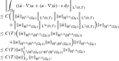
  Similarly, we can also estimate

  $$\displaystyle \begin{aligned} \left\Vert \int_{\Omega_{\mathrm F}} (u \cdot \nabla) u \cdot v \, \mathrm{d} y \right\Vert {}_{\operatorname{\mathrm{L}}^2(0,T)} \leq C (T) \Vert u \Vert_{X_T}^2\Vert v \Vert_{\operatorname{\mathrm{H}}^{1/4}(\Omega_{\mathrm F})} , \end{aligned}$$

  so we conclude that $(u\cdot \nabla ) u \in \operatorname {\mathrm {H}}^1( \operatorname {\mathrm {H}}^{-1/4}(\Omega _{\mathrm F}))$.

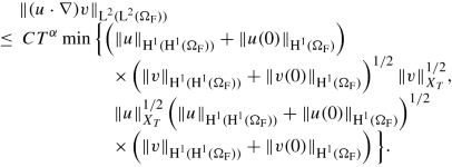
• (b) We use again Hölder’s inequality on Ω_F, the embedding $\operatorname {\mathrm {H}}^{3/2}(\Omega _{\mathrm F}) \hookrightarrow \operatorname {\mathrm {L}}^{\infty }(\Omega _{\mathrm F})$ and interpolation to estimate

  $$\displaystyle \begin{aligned} \begin{array}{rcl} & \Vert( u \cdot \nabla) v \Vert_{\operatorname{\mathrm{L}}^2(\Omega_{\mathrm F})} &\displaystyle \leq C \Vert u \Vert_{\operatorname{\mathrm{L}}^{\infty}(\Omega_{\mathrm F})} \Vert \nabla v \Vert_{\operatorname{\mathrm{L}}^2(\Omega_{\mathrm F})} \\ & &\displaystyle \leq C \Vert u \Vert_{\operatorname{\mathrm{H}}^{3/2}(\Omega_{\mathrm F})} \Vert v \Vert_{\operatorname{\mathrm{H}}^1(\Omega_{\mathrm F})} \\ & &\displaystyle \leq C \Vert u \Vert_{\operatorname{\mathrm{H}}^2(\Omega_{\mathrm F})}^{1/2} \Vert u \Vert_{\operatorname{\mathrm{H}}^1(\Omega_{\mathrm F})}^{1/2} \Vert v \Vert_{\operatorname{\mathrm{H}}^1(\Omega_{\mathrm F})} . \end{array} \end{aligned} $$

  Now, Hölder’s inequality on (0, T) together with (A.2) for q = 6, s = 1∕3 and σ = 1 implies

  

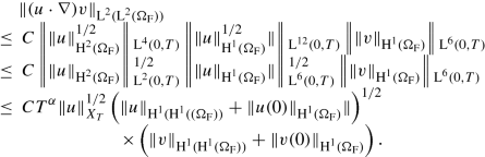
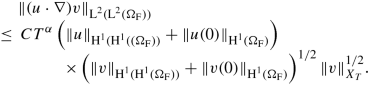
  Similarly, we obtain together with $\operatorname {\mathrm {H}}^{1/2}(\Omega _{\mathrm F}) \hookrightarrow \operatorname {\mathrm {L}}^4(\Omega _{\mathrm F})$ that

  $$\displaystyle \begin{aligned} \begin{array}{rcl} \Vert( u \cdot \nabla) v \Vert_{\operatorname{\mathrm{L}}^2(\Omega_{\mathrm F})} & \leq&\displaystyle C \Vert u \Vert_{\operatorname{\mathrm{L}}^{4}(\Omega_{\mathrm F})} \Vert \nabla v \Vert_{\operatorname{\mathrm{L}}^{4}(\Omega_{\mathrm F})} \\ & \leq &\displaystyle C \Vert u \Vert_{\operatorname{\mathrm{H}}^{1}(\Omega_{\mathrm F})} \Vert v \Vert_{\operatorname{\mathrm{H}}^{1}(\Omega_{\mathrm F})}^{1/2} \Vert v \Vert_{\operatorname{\mathrm{H}}^{2}(\Omega_{\mathrm F})}^{1/2} \end{array} \end{aligned} $$

  and hence

  

□

Lemma 6

Let u, v, w ∈ X _T . Then, there exists some α > 0 such that

Proof

For the second term, we use Hölder’s inequality, the embedding $\operatorname {\mathrm {H}}^{1/2}(\Omega _{\mathrm F}) \hookrightarrow \operatorname {\mathrm {L}}^4(\Omega _{\mathrm F})$ and interpolation to estimate

$$\displaystyle \begin{aligned} \begin{array}{rcl} & &\displaystyle \int_0^t \int_{\Omega_{\mathrm F}} \vert (\dot{u} \cdot \nabla) v \cdot \dot{w} \vert \, \mathrm{d} y \mathrm{d} s \\ & \leq &\displaystyle C \int_0^t \Vert \dot{u} \Vert_{\operatorname{\mathrm{L}}^4(\Omega_{\mathrm F})} \Vert \nabla v \Vert_{\operatorname{\mathrm{L}}^{2}(\Omega_{\mathrm F})} \Vert \dot{w} \Vert_{\operatorname{\mathrm{L}}^4(\Omega_{\mathrm F})} \, \mathrm{d} s \\ & \leq &\displaystyle C \int_0^t \Vert \dot{u} \Vert_{\operatorname{\mathrm{H}}^{1/2}(\Omega_{\mathrm F})} \Vert \nabla v \Vert_{\operatorname{\mathrm{L}}^{2}(\Omega_{\mathrm F})} \Vert \dot{w} \Vert_{\operatorname{\mathrm{H}}^{1/2}(\Omega_{\mathrm F})} \, \mathrm{d} s \\ & \leq &\displaystyle C \int_0^t \Vert \dot{u} \Vert_{\operatorname{\mathrm{L}}^2(\Omega_{\mathrm F})}^{1/2} \Vert \dot{u} \Vert_{\operatorname{\mathrm{H}}^1(\Omega_{\mathrm F})}^{1/2} \Vert v \Vert_{\operatorname{\mathrm{H}}^1(\Omega_{\mathrm F})} \Vert \dot{w} \Vert_{\operatorname{\mathrm{H}}^1(\Omega_{\mathrm F})} \, \mathrm{d} s . \end{array} \end{aligned} $$

Now, we apply again Hölder’s inequality on (0, T) together with the embedding $\operatorname {\mathrm {C}}^0(0,T) \hookrightarrow \operatorname {\mathrm {L}}^4(0,T)$ and (A.2) for q = 8, s = 3∕8 and σ = 1 and obtain

We can estimate the first term similarly. For the last term, we make use of the same tools to estimate

□

1.3 Approximation of Data

We define

$$\displaystyle \begin{aligned} A:= \operatorname{\mathrm{H}}^{2}(\Omega_{\mathrm F}) \times \operatorname{\mathrm{H}}^1(\Omega_{\mathrm F}) \times \operatorname{\mathrm{H}}^1(\Omega_{\mathrm F}) \times \operatorname{\mathrm{H}}^{2}(\Omega_{\mathrm S}) \times \operatorname{\mathrm{H}}^{1}(\Omega_{\mathrm S}) \times \operatorname{\mathrm{L}}^2(\Omega_{\mathrm S}) \end{aligned}$$

and

$$\displaystyle \begin{aligned} \begin{array}{rcl} \tilde{A} & := &\displaystyle \operatorname{\mathrm{H}}^{5/2+1/16}(\Omega_{\mathrm F}) \times \operatorname{\mathrm{H}}^1(\Omega_{\mathrm F}) \times \operatorname{\mathrm{H}}^{3/2+1/16}(\Omega_{\mathrm F}) \\ & &\displaystyle \times \operatorname{\mathrm{H}}^{5/2+1/16}(\Omega_{\mathrm S}) \times \operatorname{\mathrm{H}}^{3/2+1/16}(\Omega_{\mathrm S}) \times \operatorname{\mathrm{H}}^{1/2+1/16}(\Omega_{\mathrm S}). \end{array} \end{aligned} $$

Now, we want to show the following approximation result:

Lemma 7

For given

$$\displaystyle \begin{aligned} \begin{array}{rcl} d& :=&\displaystyle (u_0,u_1, p_0, \xi_0, \xi_1, \xi_2, f) \\ & \in &\displaystyle A \times\left( \operatorname{\mathrm{L}}^2(\operatorname{\mathrm{H}}^{1/2+1/16}(\Omega_{\mathrm F}))\cap \operatorname{\mathrm{H}}^1(\operatorname{\mathrm{H}}^{-1/2+1/16}(\Omega_{\mathrm F})) \right) \end{array} \end{aligned} $$

satisfying (4), there exists a sequence

$$\displaystyle \begin{aligned} d_n:= (u_0^n,u_1^n, p_0^n, \xi_0^n, \xi_1^n, \xi_2^n, f^n) \in \tilde{A} \times \left(\operatorname{\mathrm{C}}^\infty(\operatorname{\mathrm{H}}^{1/2+1/16}(\Omega_{\mathrm F})) \right), \end{aligned}$$

which satisfies (4) for all $n \in \mathbb {N}$ and which converges to d in

$$\displaystyle \begin{aligned} A \times \left( \operatorname{\mathrm{L}}^2(\operatorname{\mathrm{H}}^{1/2+1/16}(\Omega_{\mathrm F}))\cap \operatorname{\mathrm{H}}^1(\operatorname{\mathrm{H}}^{-1/2+1/16}(\Omega_{\mathrm F})) \right). \end{aligned}$$

Proof

To construct such a sequence, we proceed in the following steps:

• (1) As $u_1 \in \operatorname {\mathrm {H}}^1(\Omega _{\mathrm F})$ with $\operatorname {{\mathrm {div}}}(u_1)=0$ in Ω_F and u ₁|_{∂ Ω} = 0 is already satisfied, we set $u_1^n:=u_1$ for all $n \in \mathbb {N}$.

• (2) Since $\xi _2 \in \operatorname {\mathrm {L}}^2(\Omega _{\mathrm S})$ and $\operatorname {\mathrm {C}}_0^{\infty }(\Omega _{\mathrm S})$ is dense in $\operatorname {\mathrm {L}}^2(\Omega _{\mathrm S})$, we can find a sequence $(\hat {\xi }_2^n) \subset \operatorname {\mathrm {C}}_0^{\infty }(\Omega _{\mathrm S})$ such that $\lim _{n \to \infty } \hat {\xi }_2^n=\xi _2$ in $\operatorname {\mathrm {L}}^2(\Omega _{\mathrm S})$. To modify this sequence such that it satisfies the compatibility condition on ∂ Ω_S, we first define the sets

  $$\displaystyle \begin{aligned} (\partial\Omega_{\mathrm S})^n:=\left\{y \in \Omega_{\mathrm S}: \text{dist}(y, \partial\Omega_{\mathrm S}) < \frac{1}{2^n} \right\} \end{aligned}$$

  for $n \in \mathbb {N}$. Then, we can find a sequence $(\varphi ^n) \subset \operatorname {\mathrm {C}}^{\infty }(\Omega _{\mathrm S})$ such that

  $$\displaystyle \begin{aligned} \begin{array}{rcl} \varphi^n(y)= \begin{cases} 1 & \text{if } y \in (\partial\Omega_{\mathrm S})^{n+1}, \\ 0 & \text{if } y \in \Omega_{\mathrm S} \setminus (\partial\Omega_{\mathrm S})^{n}. \end{cases} \end{array} \end{aligned} $$

  Now, let $u_1^E \in \operatorname {\mathrm {H}}^1(\Omega )$ denote an extension of u ₁ to Ω, and set

  $$\displaystyle \begin{aligned} \xi_2^n:=\hat{\xi}_2^n + \varphi^n u_1^E \in \operatorname{\mathrm{H}}^1(\Omega_{\mathrm S}). \end{aligned}$$

  Then, $\xi _2^n \vert _{\partial \Omega _{\mathrm S}} = u_1 \vert _{\partial \Omega _{\mathrm S}}$ and

  $$\displaystyle \begin{aligned} \Vert \varphi^n u_1^E\Vert_{\operatorname{\mathrm{L}}^2(\Omega_{\mathrm S})} \leq C \Vert \varphi^n \Vert_{\operatorname{\mathrm{L}}^3(\Omega_{\mathrm S})} \Vert u_1^E \Vert_{\operatorname{\mathrm{L}}^6(\Omega_{\mathrm S})} \leq C \vert (\partial\Omega_{\mathrm S})^n \vert^{1/3} \Vert u_1^E \Vert_{\operatorname{\mathrm{H}}^{1}(\Omega_{\mathrm S})} \to 0, \end{aligned}$$

  so we get that $\lim _{n \to \infty } \xi _2^n=\xi _2$ in $\operatorname {\mathrm {L}}^2(\Omega _{\mathrm S})$.

• (3) Since $\xi _0\vert _{\partial \Omega _{\mathrm S}} \in \operatorname {\mathrm {H}}^{3/2}(\partial \Omega _{\mathrm S})$, we can choose a sequence $(g^n)\subset \operatorname {\mathrm {H}}^{2+1/16}(\partial \Omega _{\mathrm S})$ such that $\lim _{n \to \infty } g^n = \xi _0\vert _{\partial \Omega _{\mathrm S}}$ in $\operatorname {\mathrm {H}}^{3/2}(\partial \Omega _{\mathrm S})$. Because of

  $$\displaystyle \begin{aligned} \operatorname{{\mathrm{div}}} (\Sigma(\xi_0))=\xi_2, \end{aligned}$$

  we can construct a sequence $(\xi _0^n) \subset \operatorname {\mathrm {H}}^{5/2+1/16}(\Omega _{\mathrm S})$ which satisfies $\lim _{n \to \infty } \xi _0^n = \xi _0$ in $\operatorname {\mathrm {H}}^2(\Omega _{\mathrm S})$ by solving the Dirichlet problem

  $$\displaystyle \begin{aligned} \begin{cases} \begin{array}{rcll} \operatorname{{\mathrm{div}}} (\Sigma(\xi_0^n))&=&\xi_2^n & \text{in } \Omega_{\mathrm S} ,\\ \xi_0^n &=& g^n &\text{on } \partial\Omega_{\mathrm S}, \end{array} \end{cases} \end{aligned}$$

  and using Theorem 4 for both s = 3∕2 + 1∕16 and s = 1.

• (4) Since $\operatorname {\mathrm {H}}^{1/2+1/16}(\Omega _{\mathrm F}) \hookrightarrow \operatorname {\mathrm {H}}^{-1/2+1/16}(\Omega _{\mathrm F})$ is dense, [16, Theorem 2.1] implies that we find a sequence $(\tilde {f}^n) \subset \operatorname {\mathrm {C}}^{\infty }( \operatorname {\mathrm {H}}^{1/2+1/16}(\Omega _{\mathrm F}))$ such that $\lim _{n \to \infty } \tilde {f}^n =f$ in $\operatorname {\mathrm {L}}^2( \operatorname {\mathrm {H}}^{1/2+1/16}(\Omega _{\mathrm F}))\cap \operatorname {\mathrm {H}}^1( \operatorname {\mathrm {H}}^{-1/2+1/16}(\Omega _{\mathrm F}))$. Since d solves

  $$\displaystyle \begin{aligned} \begin{cases} \begin{array}{rcll} \operatorname{{\mathrm{div}}}(\sigma(u_0,p_0))&=& u_1-f(0) &\text{in } \Omega_{\mathrm F}, \\ \operatorname{{\mathrm{div}}}(u_0)&=&0 &\text{in } \Omega_{\mathrm F} ,\\ \sigma(u_0,p_0)n &=& \Sigma(\xi_0)n &\text{on } \partial\Omega_{\mathrm S}, \\ u_0 &=&0 &\text{on } \partial\Omega, \end{array} \end{cases} \end{aligned}$$

  integration by parts shows that

  $$\displaystyle \begin{aligned} \int_{\Omega_{\mathrm F}} f(0) \, \mathrm{d} y - \int_{\Omega_{\mathrm F}} u_1 \, \mathrm{d} y =-\int_{\partial\Omega_{\mathrm S}} \sigma (u_0,p_0)N \, \mathrm{d} S(y) = \int_{\partial\Omega_{\mathrm S}} \Sigma (\xi_0)n \, \mathrm{d} S(y). \end{aligned}$$

  Therefore, we can modify $(\tilde {f}^n)$ by adding suitable constants to obtain a sequence $(f^n)\subset \operatorname {\mathrm {C}}^{\infty }( \operatorname {\mathrm {H}}^{1/2+1/16}(\Omega _{\mathrm F}))$ such that

  $$\displaystyle \begin{aligned} \int_{\Omega_{\mathrm F}} f^n(0) \, \mathrm{d} y = \int_{\partial\Omega_{\mathrm S}} \Sigma (\xi_0^n)n \, \mathrm{d} S(y) + \int_{\Omega_{\mathrm F}} u_1^n \, \mathrm{d} y \end{aligned} $$

  (A.3)

  and still lim_n→∞ f ⁿ = f in $\operatorname {\mathrm {L}}^2( \operatorname {\mathrm {H}}^{1/2+1/16}(\Omega _{\mathrm F}))\cap \operatorname {\mathrm {H}}^1( \operatorname {\mathrm {H}}^{-1/2+1/16}(\Omega _{\mathrm F}))$. Moreover, then [16, Theorem 3.1] together with

  $$\displaystyle \begin{aligned} \left(\operatorname{\mathrm{H}}^{1/2+1/16}(\Omega_{\mathrm F}), \operatorname{\mathrm{H}}^{-1/2+1/16}(\Omega_{\mathrm F})\right)_{1/2} \hookrightarrow \operatorname{\mathrm{L}}^2(\Omega_{\mathrm F}) \end{aligned}$$

  implies that

  $$\displaystyle \begin{aligned} \Vert f- f^n \Vert_{\operatorname{\mathrm{C}}^0(\operatorname{\mathrm{L}}^2(\Omega_{\mathrm F}))}\leq C\Vert f-f^n\Vert_{\operatorname{\mathrm{L}}^2(\operatorname{\mathrm{H}}^{1/2+1/16}(\Omega_{\mathrm F}))\cap \operatorname{\mathrm{H}}^1(\operatorname{\mathrm{H}}^{-1/2+1/16}(\Omega_{\mathrm F})} \to 0, \end{aligned}$$

  so in particular lim_n→∞ f ⁿ(0) = f(0) in $\operatorname {\mathrm {L}}^2(\Omega _{\mathrm F})$.

• (5) Next, we consider the Stokes problem

  $$\displaystyle \begin{aligned} \begin{cases} \begin{array}{rcll} \operatorname{{\mathrm{div}}}(\sigma(u_0^n,p_0^n))&=& u_1^n-f^n(0) &\text{in } \Omega_{\mathrm F} ,\\ \operatorname{{\mathrm{div}}}(u_0^n)&=&0 &\text{in } \Omega_{\mathrm F}, \\ \sigma(u_0^n,p_0^n)n &=& \Sigma(\xi_0^n)n &\text{on } \partial\Omega_{\mathrm S}, \\ u_0^n &=&0 &\text{on } \partial\Omega, \end{array} \end{cases} \end{aligned}$$

  for $n \in \mathbb {N}$. Note that $f^n \in \operatorname {\mathrm {C}}^{\infty }( \operatorname {\mathrm {H}}^{1/2+1/16}(\Omega _{\mathrm F}))$ implies $f^n(0) \in \operatorname {\mathrm {H}}^{1/2+1/16}(\Omega _{\mathrm F})$. Because of (A.3) together with $u_1^n \in \operatorname {\mathrm {H}}^1(\Omega _{\mathrm F})$ and $\Sigma (\xi _0^n)n \in \operatorname {\mathrm {H}}^{1+1/16}(\partial \Omega _{\mathrm S})$, we find a sequence of solutions $(u_0^n,p_0^n) \subset \operatorname {\mathrm {H}}^{5/2+1/16}(\Omega _{\mathrm F})\times \operatorname {\mathrm {H}}^{3/2+1/16}(\Omega _{\mathrm F})$ by using Theorem 3 for s = 1∕2 + 1∕16. Since

  

  for s = 0, Theorem 3 implies $\lim _{n \to \infty } u_0^n = u_0$ in $\operatorname {\mathrm {H}}^2(\Omega _{\mathrm F})$ and $\lim _{n \to \infty } p_0^n =p_0$ in $\operatorname {\mathrm {H}}^1(\Omega _{\mathrm F})$.

• (6) Finally, we set $h:= \operatorname {{\mathrm {div}}}(\Sigma (\xi _1)) \in \operatorname {\mathrm {H}}^{-1}(\Omega _{\mathrm S}))$ and consider the elliptic problem

  $$\displaystyle \begin{aligned} \begin{cases} \begin{array}{rcll} \operatorname{{\mathrm{div}}}(\Sigma(\xi_1))&=&h &\text{in } \operatorname{\mathrm{H}}^{-1}(\Omega_{\mathrm S}) ,\\ \xi_1&=&u_0 &\text{on } \partial\Omega_{\mathrm S}. \end{array} \end{cases} \end{aligned}$$

  Now, choose some sequence $(h^n) \subset \operatorname {\mathrm {L}}^2(\Omega _{\mathrm S})$ such that lim_n→∞ h ⁿ = h in $\operatorname {\mathrm {H}}^{-1}(\Omega _{\mathrm S})$, and consider the elliptic problems

  $$\displaystyle \begin{aligned} \begin{cases} \begin{array}{rcll} \operatorname{{\mathrm{div}}}(\Sigma(\xi_1^n))&=&h^n &\text{in } \Omega_{\mathrm S} ,\\ \xi_1^n&=&u_0^n &\text{on } \partial\Omega_{\mathrm S}. \end{array} \end{cases} \end{aligned}$$

  Since it follows from step 5 that $(u_0^n\vert _{\partial \Omega _{\mathrm S}}) \subset \operatorname {\mathrm {H}}^{2+1/16}(\partial \Omega _{\mathrm S})$ and $\lim _{n \to \infty } u_0^n\vert _{\partial \Omega _{\mathrm S}} = u_0\vert _{\partial \Omega _{\mathrm S}}$ in $\operatorname {\mathrm {H}}^{3/2}(\partial \Omega _{\mathrm S})$, we can use Theorem 4 for both s = 1 and s = 0 and obtain a sequence of solutions $(\xi _1^n) \subset \operatorname {\mathrm {H}}^2(\Omega _{\mathrm S})$ such that $\lim _{n \to \infty } \xi _1^n = \xi _1$ in $\operatorname {\mathrm {H}}^1(\Omega _{\mathrm S})$.

Consequently, we have found a compatible sequence

$$\displaystyle \begin{aligned} (d_n):=(u_0^n,u_1^n, p_0^n, \xi_0^n, \xi_1^n, \xi_2^n, f^n) \end{aligned}$$

approximating d in

$$\displaystyle \begin{aligned} A \times \left(\operatorname{\mathrm{L}}^2(\operatorname{\mathrm{H}}^{1/2+1/16}(\Omega_{\mathrm F}))\cap \operatorname{\mathrm{H}}^1(\operatorname{\mathrm{H}}^{-1/2+1/16}(\Omega_{\mathrm F})) \right).\end{aligned} $$

□

References

G. Avalos, P.G. Geredeli, J.T. Webster, A linearized viscous, compressible flow-plate interaction with non-dissipative coupling. J. Math. Anal. Appl. 477(1), 334–356 (2019)
S. Bechtel, M. Egert, Interpolation theory for Sobolev functions with partially vanishing trace on irregular open sets. J. Fourier Anal. Appl. 25(5), 2733–2781 (2019)
M. Boulakia, Existence of weak solutions for the three-dimensional motion of an elastic structure in an incompressible fluid. J. Math. Fluid Mech. 9(2), 262–294 (2007)
M. Boulakia, S. Guerrero, T. Takahashi, Well-posedness for the coupling between a viscous incompressible fluid and an elastic structure. Nonlinearity 32, 3548–3592 (2019)
D. Coutand, S. Shkoller, Motion of an elastic solid inside an incompressible viscous fluid. Arch. Ration. Mech. Anal. 176(1), 25–102 (2005)
D. Coutand, S. Shkoller, The interaction between quasilinear elastodynamics and the Navier-Stokes equations. Arch. Ration. Mech. Anal. 179(3), 303–352 (2006)
E. Di Nezza, G. Palatucci, E. Valdinoci, Hitchhiker’s guide to the fractional Sobolev spaces. Bull. Sci. Math. 136, 512–573 (2012)
C. Grandmont, M. Hillairet, Existence of global strong solutions to a beam-fluid interaction system. Arch. Ration. Mech. Anal. 220(3), 1283–1333 (2016)
C. Grandmont, M. Hillairet, J. Lequeurre, Existence of local strong solutions to fluid-beam and fluid-rod interaction systems. Ann. Inst. H. Poincaré Anal. Non Linéaire 36(4), 1105–1149 (2019)
G. Grubb, V. Solonnikov, Boundary Value Problems for the Nonstationary Navier-Stokes Equations treated by Pseudo-Differential Methods. Math. Scand. 69, 217–290 (1991)
P. Haupt, Continuum Mechanics and Theory of Materials (Springer, Berlin, 2002)
M. Ignatova, I. Kukavica, I. Lasiecka, A. Tuffaha, Small data global existence for a fluid-structure model. Nonlinearity 30(2), 848–898 (2017)
I. Kukavica, A. Tuffaha, Solutions to a fluid-structure interaction free boundary problem. Discrete Contin. Dyn. Syst. 32(4), 1355–1389 (2012)
I. Kukavica, A. Tuffaha, M. Ziane, Strong solutions to a Navier-Stokes-Lamé system on a domain with a nonflat boundary. Nonlinearity 24, 159–176 (2011)
I. Lasiecka, J.L. Lions, R. Triggiani, Non-homogeneous boundary value problems for second order hyperbolic operators. J. Math. Pures Appl. 65, 149–192 (1986)
J.L. Lions, E. Magenes, Non-Homogeneous Boundary Value Problems and Applications (Springer, Berlin, 1972)
B. Muha, S. Čanić, Fluid-structure interaction between an incompressible, viscous 3D fluid and an elastic shell with nonlinear Koiter membrane energy. Interfaces Free Bound. 17(4), 465–495 (2015)
J.P. Raymond, M. Vanninathan, A fluid-structure model coupling the Navier-Stokes equations and the Lamé system. J. Math. Pures Appl. 102, 546–596 (2014)
H. Triebel, Interpolation Theory, Function Spaces, Differential Operators (North-Holland Publishing Company, Amsterdam, 1978)
Acknowledgements
Michelle Luckas would like to thank the “Studienstiftung des deutschen Volkes” for academic and financial support.
Author information
Authors and Affiliations
Corresponding author
Editor information
Editors and Affiliations