Network Analysis for Economics and Finance: An Application to Firm Ownership

Abstract

In this chapter, we introduce network analysis as an approach to model data in economics and finance. First, we review the most recent empirical applications using network analysis in economics and finance. Second, we introduce the main network metrics that are useful to describe the overall network structure and characterize the position of a specific node in the network. Third, we model information on firm ownership as a network: firms are the nodes while ownership relationships are the linkages. Data are retrieved from Orbis including information of millions of firms and their shareholders at worldwide level. We describe the necessary steps to construct the highly complex international ownership network. We then analyze its structure and compute the main metrics. We find that it forms a giant component with a significant number of nodes connected to each other. Network statistics show that a limited number of shareholders control many firms, revealing a significant concentration of power. Finally, we show how these measures computed at different levels of granularity (i.e., sector of activity) can provide useful policy insights.

1 Introduction

Historically, networks have been studied extensively in graph theory, an area of mathematics. After many applications to a number of different subjects including statistical physics, health science, and sociology, over the last two decades, an extensive body of theoretical and empirical literature was developed also in economics and finance. Broadly speaking, a network is a system with nodes connected by linkages. A node can be, e.g., an individual, a firm, an industry, or even a geographical area. Correspondingly, different types of relationships have been represented as linkages. Indeed, network has become such a prominent cross-disciplinary topic [10] because it is extremely helpful to model a variety of data, even when they are big data [67]. At the same time, network analysis provides the capacity to estimate effectively the main patterns of several complex systems [66]. It is a prominent tool to better understand today’s interlinked world, including economic and financial phenomena. To mention just a few applications, networks have been used to explain the trade of goods and services [39], financial flows across countries [64], innovation diffusion among firms, or the adoption of new products [3]. Another flourishing area of research related to network is the one of social connections, which with the new forms of interaction like online communities (e.g., Facebook or LinkedIn) will be even more relevant in the future [63]. Indeed network analysis is a useful tool to understand strategic interactions and externalities [47]. Another strand of literature, following the 2007–2008 financial crisis, has shown how introducing a network approach in financial models can feature the interconnected nature of financial systems and key aspects of risk measurement and management, such as credit risk [27], counterparty risk [65], and systemic risk [13]. This network is also central to understanding the bulk of relationships that involve firms [12, 74, 70]. In this chapter, we present an application explaining step by step how to construct the network and perform some analysis, in which links are based on ownership information. Firms’ ownership structure is an appropriate tool to identify the concentration of power [7], and a network perspective is particularly powerful to uncover intricate relationships involving indirect ownership. In this context, the connectivity of a firm depends on the entities with direct shares, if these entities are themselves controlled by other shareholders, and whether they also have shares in other firms. Hence, some firms are embedded in tightly connected groups of firms and shareholders, others are relatively disconnected. The overall structure of relationships will tell whether a firm is central in the whole web of ownership system, which may have implications, for example, for foreign direct investment (FDI).

Besides this specific application, the relevance of the network view has been particularly successful in economics and finance thanks to the unique insights that this approach can provide. A variety of network measures, at a global scale, allow to investigate in depth the structure, even of networks including a large number of nodes and/or links, explaining what patterns of linkages facilitate the transmission of valuable information. Node centrality measures may well complement information provided by other node attributes or characteristics. They may enrich other settings, such as standard micro-econometric models, or they may explain why an idiosyncratic shock has different spillover effects on the overall system depending on the node that is hit. Moreover, the identification of key nodes (i.e., nodes that can reach many other nodes) can be important for designing effective policy intervention. In a highly interconnected world, for example, network analysis can be useful to map the investment behavior of multinational enterprises and analyze the power concentration of nodes in strategic sectors. It can also be deployed to describe the extension and geographical location of value chains and the changes we are currently observing with the reshoring of certain economic activities as well as the degree of dependence on foreign inputs for the production of critical technologies. The variety of contexts to which network tools can be applied and the insights that this modeling technique may provide make network science extremely relevant for policymaking. Policy makers and regulators face dynamic and interconnected socioeconomic systems. The ability to map and understand this complex web of technological, economic, and social relationships is therefore critical for taking policy decision and action—even more, in the next decades when policy makers will face societal and economic challenges such as inequality, population ageing, innovation challenges, and climate risk. Moreover, network analysis is a promising tool also for investigating the fastest-changing areas of non-traditional financial intermediation, such as peer-to-peer lending, decentralized trading, and adoption of new payment instruments.

This chapter introduces network analysis providing suggestions to model data as a network for beginners and describes the main network tools. It is organized as follows. Section 2 provides an overview of recent applications of network science in the area of economics and finance. Section 3 introduces formally the fundamental mathematical concepts of a network and some tools to perform a network analysis. Section 4 illustrates in detail the application of network analysis to firm ownership and Sect. 5 concludes.

2 Network Analysis in the Literature

In economics, a large body of literature using micro-data investigates the effects of social interactions. Social networks are important determinants to explain job opportunity [18], student school performance [20],¹ criminal behavior [18], risk sharing [36], investment decisions [51], CEO compensations of major corporations [52], corporate governance of firms [42], and investment decision of mutual fund managers [26]. However, social interaction effects are subject to significant identification challenges [61]. An empirical issue is to disentangle the network effect of each other’s behaviors from individual and group characteristics. An additional challenge is that the network itself cannot be always considered as exogenous but depends on unobservable characteristics of the individuals. To address these issues several strategies have been exploited: variations in the set of peers having different observable characteristics; instrumental variable approaches using as instrument, for example, the architecture of network itself; or modeling the network formation. See [14] and [15] for a deep discussion of the econometric framework and the identification conditions. Network models have been applied to the study of markets with results on trading outcomes and price formation corroborated by evidence obtained in laboratory [24]. Spreading of information is so important in some markets that networks are useful to better understand even market panics (see, e.g., [55]). Other applications are relevant to explain growth and economic outcome. For example, [3] find that past innovation network structures determine the process of future technological and scientific progress. Moreover, networks determine how technological advances generate positive externalities for related fields. Empirical evidences are relevant also for regional innovation policies [41]. In addition, network concepts have been adopted in the context of input–output tables, in which nodes represent the individual industries of different countries and links denote the monetary flows between industries [22], and the characterization of different sectors as suppliers to other sectors to explain aggregate fluctuations [1].²

In the area of finance,³ since the seminal work by [5] network models have been revealed suitable to address potential domino effects resulting from interconnected financial institutions. Besides the investigation of the network structure and its properties [28], this framework has been used to answer the question whether the failure of an institution may propagate additional losses in the banking system [75, 72, 65, 34]. Importantly it has been found that network topology influences contagion [43, 2]. In this stream of literature, financial institutions are usually modeled as the nodes, while direct exposures are represented by the linkages (in the case of banking institutions, linkages are the interbank loans). Some papers use detailed data containing the actual exposures and the counterparties involved in the transactions. However, those data are usually limited to the banking sector of a single country (as they are disclosed to supervisory authorities) or a specific market (e.g., overnight interbank lending [53]). Unfortunately, most of the time such a level of detail is not available, and thus various methods have been developed to estimate networks, which are nonetheless informative for micro- and macro-prudential analysis (see [8] for an evaluation of different estimation methodologies). The mapping of balance sheet exposures and the associated risks through networks is not limited to direct exposures but has been extended to several financial instruments and common asset holdings such as corporate default swaps (CDS) exposures [23], bail-inable securities [50], syndicated loans [48, 17], and inferred from market price data [62, 13]. Along this line, when different financial instruments are considered at the same time, financial institutions are then interconnected in different market segments by multiple layer networks [11, 60, 68]. Network techniques are not limited to model interlinkages across financial institutions at micro level. Some works consider as a node the overall banking sector of a country to investigate more aggregated effects [31] and the features of the global banking network [64]. Other papers have applied networks to cross-border linkages and interdependencies of the international financial system, such as the international trade flows [38, 39] and cross-border exposures by asset class (foreign direct investment, portfolio equity, debt, and foreign exchange reserves) [56]. Besides the different level of aggregation to which a node can be defined, also a heterogeneous set of agents can be modeled in a network framework. This is the approach undertaken in [13], where nodes are hedge funds, banks, broker/dealers, and insurance companies, and [21] that consider the institutional sectors of the economy (non-financial corporations, monetary financial institutions, other financial institutions, insurance corporations, government, households, and the rest of the world).

Both in economics and finance, the literature has modeled firms as nodes considering different types of relationships, such as production, supply, or ownership, which may create an intricate web of linkages. The network approach has brought significant insights in the organization of production and international investment. [12] exploit detailed data on production network in Japan, showing that geographic proximity is important to understand supplier–customer relationships. The authors, furthermore, document that while suppliers to well-connected firms have, on average, relatively few customers, suppliers to less connected firms have, on average, many customers (negative degree assortativity). [6] exploring the structure of national and multinational business groups find a positive relationship between a groups’ hierarchical complexity and productivity. [32] provide empirical evidence that parent companies and affiliates tend to be located in proximity over a supply chain. Starting with the influential contribution of [58], an extensive body of literature in corporate finance investigates the various types of firm control. Important driving forces are country legal origin and investor protection rights [58, 59]. In a recent contribution, [7] describe extensively corporate control for a large number of firms, documenting persistent differences across countries in corporate control and the importance of various institutional features. [74] investigate the network structure of transnational corporations and show that it can be represented as a bow-tie structure with a relatively small number of entities in the core. In a related paper, [73] study the community structure of the global corporate network identifying the importance of the geographic location of firms. A strong concentration of corporate power is documented also in [70]. Importantly, they show that parent companies choose indirect control when located in countries with better financial institutions and more transparent forms of corporate governance. Formal and informal networks may have even performance consequences [49], affect governance mechanisms [42], and lead to distortions in director selection [57]. For example, in [42] social connections between executives and directors undermine independent corporate governance, having a negative impact on firm value. In the application of this chapter, we focus on ownership linkages following [74, 70], and we provide an overview of the worldwide network structure and the main patterns of control.

This section does not provide a comprehensive literature review, but rather it aims to give an overview of the variety of applications using network analysis and the type of insights it may suggest. In this way we hope to help the reader to think about his own data as a network.

3 Network Analysis

This section formally introduces graphs⁴ and provides an overview of standard network metrics, proceeding from local to more global measures.

A graph $G = \left ( V, E \right )$ consists of a set of nodes V  and a set of edges E ⊆ V ² connecting the nodes. A graph G can conveniently be represented by a matrix $W \in \mathbb {R}^{n \times n}$, where $n \in \mathbb {N}$ denotes the number of nodes in G and the matrix element w _ij represents the edge from node i to node j. Usually w _ij = 0 is used to indicate a non-existing edge. Graphs are furthermore described by the following characteristics (see also Figs. 1 and 2):

• A graph G is said to be undirected, if there is no defined edge direction. This especially means w _ij = w _ji for all i, j = 1, …, n, and the matrix W is symmetric. Conversely, if we distinguish between the edge w _ij (from node i to node j) and the edge w _ji (from node j to node i), the graph is said to be directed.⁵

  Fig. 1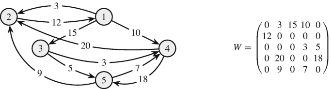

  

  Example of a directed and weighted graph

  Fig. 2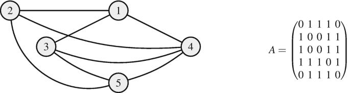

  

  Example of an undirected and unweighted graph

• If a graph describes only the existence of edges, i.e., $W \in \left \{ 0, 1 \right \}^{n \times n}$, the graph is said to be unweighted. In this case, the matrix W is called the adjacency matrix, commonly denoted by A. Note that for every graph W there exists an adjacency matrix $A \in \left \{ 0, 1 \right \}^{n \times n}$, defined by . Conversely, if the edges w _ij carry weights, i.e., $w_{ij} \in \mathbb {R}$, the graph G is said to be weighted.⁶

While a visual inspection can be very helpful for small networks, this approach quickly becomes difficult as the number of nodes increases. Especially in the era of big data, more sophisticated techniques are required. Thus, various network metrics and measures have been developed to help describe and analyze complex networks. The most common ones are explained in the following.

Most networks do not exhibit self-loops, i.e., edges connecting a node with itself. For example, in social networks it makes no sense to model a person being friends with himself or in financial networks a bank lending money to itself. Therefore, in the following we consider networks without self-loops. It is however straightforward to adapt the presented network statistics to graphs containing self-loops. Moreover, we consider the usual case of networks comprising only positive weights, i.e., $W \in \mathbb {R}_{\ge 0}^{n \times n}$. Adaptations to graphs with negative weights are however also possible. Throughout this section let W ^(dir) denote a directed graph and W ^(undir) an undirected graph.

The network density $\rho \in \left [0, 1\right ]$ is defined as the ratio of the number of existing edges and the number of possible edges, i.e., for W ^(dir) and W ^(undir), the density is given by:

(1)

The density of a network describes how tightly the nodes are connected. Regarding financial networks, the density can also serve as an indicator for diversification. The higher the density, the more edges, i.e., the more diversified the investments. For example, the graph pictured in Fig. 1 has a density of 0.5, indicating that half of all possible links, excluding self-loops, exist.

While the density summarizes the overall interconnectedness of the network, the degree sequence describes the connectivity of each node. The degree sequence $d = \left ( d_1, \ldots , d_n \right ) \in \mathbb {N}_0^n$ of W ^(dir) and W ^(undir) is given for all i = 1, …, n by:

(2)

For a directed graph W ^(dir) we can differentiate between incoming and outgoing edges and thus define the in-degree sequence d ⁽ⁱⁿ⁾ and the out-degree sequence d ^(out) as:

(3)

The degree sequence shows how homogeneously the edges are distributed among the nodes. Financial networks, for example, are well-known to include some well-connected big intermediaries and many small institutions and hence exhibit a heterogeneous degree sequence. For example, for the graph pictured in Fig. 1, we get the following in- and out-degree sequences, indicating that node 4 has the highest number of connections, 3 incoming edges, and 2 outgoing edges:

$$\displaystyle \begin{aligned} d_{W^{\mathrm{(dir)}}}^{\mathrm{(in)}} &= \left( d_{1, W^{\mathrm{(dir)}}}^{\mathrm{(in)}}, d_{2, W^{\mathrm{(dir)}}}^{\mathrm{(in)}} , \ldots, d_{5, W^{\mathrm{(dir)}}}^{\mathrm{(in)}} \right) = \left( 1, 3, 1, 3, 2 \right) , \qquad \\ d_{W^{\mathrm{(dir)}}}^{\mathrm{(out)}} &= \left( d_{1, W^{\mathrm{(dir)}}}^{\mathrm{(out)}}, d_{2, W^{\mathrm{(dir)}}}^{\mathrm{(out)}} , \ldots, d_{5, W^{\mathrm{(dir)}}}^{\mathrm{(out)}} \right) = \left( 3, 1, 2, 2, 2 \right) . \end{aligned} $$

(4)

Similarly, for weighted graphs, the distribution of the weight among the nodes is described by the strength sequence $s = \left ( s_1, \ldots , s_n \right ) \in \mathbb {R}_{ \ge 0}^n$ and is given for all i = 1, …, n by:

$$\displaystyle \begin{aligned} s_{i, W^{\mathrm{(dir)}}} = \sum_{j = 1}^n w_{ij} + w_{ji}, \qquad s_{i, W^{\mathrm{(undir)}}} = \sum_{j = 1}^n w_{ij} . \end{aligned} $$

(5)

In addition, for the weighted and directed graph W ^(dir), we can differentiate between the weight that flows into a node and the weight that flows out of it. Thus, the in-strength sequence s ⁽ⁱⁿ⁾ and the out-strength sequence s ^(out) are defined for all i = 1, …, n as:

$$\displaystyle \begin{aligned} s_{i, W^{\mathrm{(dir)}}}^{\mathrm{(in)}} = \sum_{j = 1}^n w_{ji} , \qquad s_{i, W^{\mathrm{(dir)}}}^{\mathrm{(out)}} = \sum_{j = 1}^n w_{ij} . \\ \end{aligned} $$

(6)

For example, for the graph pictured in Fig. 1, we get the following in- and out-strength sequences:

$$\displaystyle \begin{aligned} s_{W^{\mathrm{(dir)}}}^{\mathrm{(in)}} &= \left( s_{1, W^{\mathrm{(dir)}}}^{\mathrm{(in)}}, s_{2, W^{\mathrm{(dir)}}}^{\mathrm{(in)}} , \ldots, s_{5, W^{\mathrm{(dir)}}}^{\mathrm{(in)}} \right) = \left( 12, 32, 15, 20, 23 \right) , \qquad \\ s_{W^{\mathrm{(dir)}}}^{\mathrm{(out)}} &= \left( s_{1, W^{\mathrm{(dir)}}}^{\mathrm{(out)}}, s_{2, W^{\mathrm{(dir)}}}^{\mathrm{(out)}} , \ldots, s_{5, W^{\mathrm{(dir)}}}^{\mathrm{(out)}} \right) = \left( 28, 12, 8, 38, 16 \right) . \end{aligned} $$

(7)

Node 2 is absorbing more weight than all other nodes with an in-strength of 32, while node 4 is distributing more weight than all other nodes with an out-strength of 38.

The homogeneity of a graph in terms of its edges or weights is measured by the assortativity. Degree (resp. strength) assortativity is defined as Pearson’s correlation coefficient of the degrees (resp. strengths) of connected nodes. Likewise, we can define the in- and out-degree assortativity and in- and out-strength assortativity. Negative assortativity, also called disassortativity, indicates that nodes with few edges (resp. low weight) tend to be connected with nodes with many edges (resp. high weight) and vice versa. This is, for example, the case for financial networks, where small banks and corporations maintain financial relationships (e.g., loans, derivatives) rather with big well-connected financial institutions than between themselves. Positive assortativity, on the other hand, indicates that nodes tend to be connected with nodes that have a similar degree (resp. similar weight). For example, the graph pictured in Fig. 1 has a degree disassortativity of − 0.26 and a strength disassortativity of − 0.24, indicating a slight heterogeneity of the connected nodes in terms of their degrees and strengths.

The importance of a node is assessed through centrality measures. The three most prominent centrality measures are betweenness, closeness, and eigenvector centrality and can likewise be defined for directed and undirected graphs. (Directed or undirected) betweenness centrality b _i of vertex i is defined as the sum of fractions of (resp. directed or undirected) shortest paths that pass through vertex i over all node pairs, i.e.:

$$\displaystyle \begin{aligned} b_i = \sum_{j, h =1}^n \frac{s_{jh} \left( i \right) }{s_{jh} }, \end{aligned} $$

(8)

where $s_{jh} \left ( i \right )$ is the number of shortest paths between vertices j and h that pass through vertex i, s _jh is the number of shortest paths between vertices j and h, and with the convention that $s_{jh} \left ( i \right ) / s_{jh} = 0$ if there is no path connecting vertices j and h. For example, the nodes of the graph pictured in Fig. 1 have betweenness centralities $b = \left ( b_1, b_2, \ldots , b_5 \right ) = \left ( 5, 5, 1, 2, 1 \right )$, i.e., nodes 1 and 2 are the most powerful nodes as they maintain the highest ratio of shortest paths passing through them.

(Directed or undirected) closeness centrality c _i of vertex i is defined as the inverse of the average shortest path (resp. directed or undirected) between vertex i and all other vertices, i.e.:

$$\displaystyle \begin{aligned} c_i = \frac{n-1 }{\sum_{j \ne i} d_{ij} }, \end{aligned} $$

(9)

where d _ij denotes the length of the shortest path from vertex i to vertex j. For example, the nodes of the graph pictured in Fig. 1 have closeness centralities $c = \left ( c_1, c_2, \ldots , c_5 \right ) = \left ( 0.80, 0.50, 0.57, 0.57, 0.57 \right )$. Note that in comparison to betweenness centrality, node 1 is closer to other nodes than node 2 as it has more outgoing edges.

Eigenvector centrality additionally accounts for the importance of a node’s neighbors. Let λ denote the largest eigenvalue of the adjacency matrix a and e the corresponding eigenvector, i.e., λa = ae holds. The eigenvector centrality of vertex i is given by:

$$\displaystyle \begin{aligned} e_i = \frac{1}{\lambda} \sum_{j} a_{ij} e_j . \end{aligned} $$

(10)

The closer a node is connected to other important nodes, the higher is its eigenvector centrality. For example, the nodes of the graph pictured in Fig. 2 (representing the undirected and unweighted version of the graph in Fig. 1) have eigenvector centralities e = (e ₁, e ₂, …, e ₅) = (0.19, 0.19, 0.19, 0.24, 0.19), i.e., node 4 has the highest eigenvector centrality. Taking a look at the visualization in Fig. 2, this result is no surprise. In fact node 4 is the only node that is directly connected to all other nodes, naturally rendering it the most central node.

Another interesting network statistic is the clustering coefficient, which indicates the tendency to form triangles, i.e., the tendency of a node’s neighbors to be also connected to each other. An intuitive example for a highly clustered network are friendship networks, as two people with a common friend are likely to be friends as well. Let a denote the adjacency matrix of an undirected graph. The clustering coefficient C _i of vertex i is defined as the ratio of realized to possible triangles formed by i:

$$\displaystyle \begin{aligned} C_i = \frac{ \left( a^3 \right)_{ii} }{ d_i \left( d_i -1 \right) }, \end{aligned} $$

(11)

where d _i denotes the degree of node i. For example, the nodes of the graph pictured in Fig. 2 have clustering coefficients C = (C ₁, C ₂, …, C ₅) = (0.67, 0.67, 0.67, 0.67, 0.67). This can be easily verified via the visualization in Fig. 2. Nodes 1, 2, 3, and 5 form each part of 2 triangles and have 3 edges, which give rise to a maximum of 3 triangles (C ₁ = 2∕3). Node 4 forms part of 4 triangles and has 4 links, which would make 6 triangles possible (C ₄ = 4∕6). For an extension of the clustering coefficient to directed and weighted graphs, the reader is kindly referred to [37].

Furthermore, another important strand of literature works on community detection. Communities are broadly defined as groups of nodes that are densely connected within each group and sparsely between the groups. Identifying such groupings can provide valuable insight since nodes of the same community often have further features in common. For example, in social networks, communities are formed by families, sports clubs, and educationally or professionally linked colleagues; in biochemical networks, communities may constitute functional modules; and in citation networks, communities indicate a common research topic. Community detection is a difficult and often computationally intensive task. Many different approaches have been suggested, such as the minimum-cut method, modularity maximization, and the Girvan–Newman algorithm, which identifies communities by iteratively cutting the links with the highest betweenness centrality. Detailed information on community detection and comparison of different approaches are available in, e.g., [67] and to [30].

One may be interested in separating the nodes in communities that are tightly connected inside but with a few links between nodes that are part of different communities. Furthermore, we can identify network components that are of special interest. The most common components are the largest weakly connected component (LWCC) and largest strongly connected component (LSCC). The LWCC is the largest subset of nodes, such that within the subset there exists an undirected path from each node to every other node. The LSCC is the largest subset of nodes, such that within the subset there exists a directed path from each node to every other node.

The concepts and measures we had presented are general and can be applied to any network.⁷ However, their interpretation depends on the specific context of application. A knowledge of the underlined economic/financial phenomenon is also necessary before starting to model the raw data as a network. When building a network, a preliminary exploration of the data helps to control or mitigate errors that arise from working with data collected in real-world settings (i.e., missing data, measurement errors…). Data quality, or at least awareness of data limitations, is important to perform an accurate network analysis and to draw credible inferences and conclusions. When performing a network analysis, it is also important to remind that the line of investigation depends on the network under consideration: in some cases it could be more relevant to study deeply centrality measures while in others to detect communities.

For data processing and implementation of network measures, several software are available. R, Python, and MATLAB include tools and packages that allow the computation of the most popular measures and network analysis, while Gephi and Pajek are open-source options for exploring visually a network.

4 Network Analysis: An Application to Firm Ownership

In this section we present an application of network analysis to firm ownership, that is, the shareholders of firms. We first describe the data and how the network was built. Then we show the resulting network structure and comment the main results.

4.1 Data

Data on firm ownership are retrieved from Orbis compiled by Bureau van Dijk (a Moody’s Analytics Company). Orbis provides detailed firm’s ownership information. Bureau van Dijk collects ownership information directly from multiple sources including the company (annual reports, web sites, private correspondence) and official regulatory bodies (when they are in charge of collecting this type of information) or from the associated information providers (who, in turn, have collected it either directly from the companies or via official bodies). It includes mergers and acquisitions when completed. Ownership data include for each firm the list of shareholders and their shares. They represent voting rights, rather than cash-flow rights, taking into account dual shares and other special types of share. In this application, we also consider the country of incorporation and the entity type.⁸ In addition, we collect for each firm the primary sector of activity (NACE Revision 2 codes)⁹ and, when available, financial data (in this application we restrict our interest to total assets, equity, and revenues). Indeed Orbis is widely used in the literature for the firms’ balance sheets and income statements, which are available at an annual frequency. All data we used refer to year 2016.

4.2 Network Construction

In this application we aim to construct an ownership network that consists of a set of nodes representing different economic actors, as listed in footnote 8, and a set of directed weighted links denoting the shareholding positions between the nodes.¹⁰ More precisely, a link from node A to node B with weight x means that A holds x% of the shares of B. This implies that the weights are restricted to the interval [0, 100].¹¹

Starting from the set of data available in Orbis, we extract listed firms.¹² This set of nodes can be viewed as the seed of the network. Any other seed of interest can of course be chosen likewise. Then, using the ownership information (the names of owners and their respective ownership shares) iteratively, the network is extended by integrating all nodes that are connected to the current network through outgoing or incoming links.¹³ At this point, we consider all entities and both the direct and the total percentage figures provided in the Orbis database. This process stops when all outgoing and incoming links of all nodes lead to nodes which already form part of the network. To deal with missing and duplicated links, we subsequently perform the following adjustments: (1) in case Orbis lists multiple links with direct percentage figures from one shareholder to the same firm, these shares are aggregated into a single link; (2) in case direct percentage figures are missing, the total percentage figures are used; (3) in case both the direct and total percentage figures are missing, the link is removed; and (4) when shareholders of some nodes jointly own more than 100%, the concerned links are proportionally rescaled to 100%. From the resulting network, we extract the largest weakly connected component (LWCC) that comprises over 98% of the nodes w.r.t. the network derived so far.

The resulting sample includes more than 8.1 million observations, of which around 4.6 million observations are firms (57%).¹⁴ The majority of firms are active in the sectors wholesale and retail trade; professional, scientific, and technical activities; and real estate activities (see Table 5). When looking at the size of sectors with respect to accounting the variables, the picture changes. In terms of total assets and equity, the main sectors are financial and insurance activities and manufacturing, while in terms of revenues, as expected, manufacturing and wholesale and retail trade have the largest share. We also report the average values, which again display a significant variation between sectors. Clearly the overall numbers hide a wide heterogeneity within sector, but some sectors are dominated by very large firms (e.g., mining and quarrying), while in others micro or small firms are prevalent (e.g., wholesale and retail trade). The remaining sample includes entities of various types, such as individuals, which do not have to report a balance sheet. Nodes are from all over the world, but with a prevalence from developed countries and particularly from those having better reporting standards.

A visualization of the entire network with 8.1 million nodes is obviously not possible here. However, to still gain a better idea of the structure of the network, Fig. 3 visualizes part of the network, namely, the IN component (see Sect. 4.4).¹⁵ It is interesting to note that the graph shows some clear clusters for certain countries.

Fig. 3

Visualization of the IN component (see Sect. 4.4) and considering only the links with the weight of at least 1%. Countries that contain a substantial part of the nodes of this subgraph are highlighted in individual colors according to the legend on the right-hand side. This graph was produced with Gephi

4.3 Network Statistics

The resulting ownership network constitutes a complex network with millions of nodes and links. This section demonstrates how network statistics can help us gain insight into such opaque big data structure.

Table 1 summarizes the main network characteristics. The network includes more than 8.1 million of nodes and 10.4 million of links. This also implies that the ownership network is extremely sparse with a density of less 1E-6. The average share is around 38.0% but with a substantial heterogeneity across links.

Table 1 General characteristics of the ownership network

Table 2 Centrality measures: summary statistics

Table 2 shows the summary statistics of the network measures computed at node level. The ownership network is characterized by a high heterogeneity: there are firms wholly owned by a single shareholder (i.e., owning 100% of the shares) and firms with a dispersed ownership in which some shareholders own a tiny percentage. These features are reflected in the in-degree and in-strength. Correspondingly, there are shareholders with just a participation in a unique firm and others with shares in many different firms (see the out-degree and out-strength).

Table 3 Size of the components of the bow-tie structure

To gain further insights, we investigate the in-degree and out-degree distribution, that is, an analysis frequently used in complex networks. Common degree distributions identified in real-world networks are Poisson, exponential, or power-law distributions. Networks with power-law degree distribution, usually called scale-free networks, show many end nodes, other nodes with a low degree, and a handful of very well-connected nodes.¹⁶ Since power laws show a linear relationship in logarithmic scales, it is common to visualize the degree distributions in the form of the complementary cumulative distribution function (CDF) in a logarithmic scale. Figure 4 displays the in- and out-degree distribution in panels (a) and (b), respectively. Both distributions show the typical behavior of scale-free networks, with the majority of nodes having a low degree and a few nodes having a large value. When considering the in-degree distribution, we can notice that there are 94% of the nodes with an in-degree equal or lower than 3. While this is partially explained by the presence of pure investors, when excluding these nodes from the distribution, the picture does not change much (90% of the nodes have an in-degree equal or lower than 3). This provides further evidence that the majority of firms are owned by very few shareholders, while a limited number of firms, mainly listed firms, are owned by many shareholders. A similar pattern is observed for the out-degree; indeed many shareholders invest in a limited number of firms, while few shareholders own shares in a large number of firms. This is the case of investment funds that aim to have a diversified portfolio.¹⁷

Fig. 4

Degree distribution in log–log scale. Panel a (Panel b) shows the in-degree (out-degree) distribution. The y-axis denotes the complementary cumulative distribution function

Concerning the centrality measures, the summary statistics in Table 2 suggest a high heterogeneity across nodes. It is also interesting to notice that centrality measures are positively correlated with financial data. Entities having high values of centrality are usually financial entities and institutional shareholders, such as mutual funds, banks, and private equity firms. In some cases, entities classified as states and governments have high values possibly due to state-owned enterprises, which in some countries are still quite diffused in certain sector of the economy.

4.4 Bow-Tie Structure

The ownership networks can be split into the components of a bow-tie structure (see, e.g., [74, 46]), as pictured in Fig. 5. Each component identifies a group of entities with a specific structure of interactions. In the center we have a set of closely interconnected firms forming the largest strongly connected component (LSCC). Next, we can identify all nodes that can be reached via a path of outgoing edges starting from the LSCC. These nodes constitute the OUT component and describe firms that are at least partially owned by the LSCC. Likewise, all nodes that can be reached via a path of incoming edges leading to the LSCC are grouped in the IN component. These nodes own at least partially the LSCC and thus indirectly also the OUT component. Nodes that lie on a path connecting the IN with the OUT component form the Tubes. All nodes that are connected through a path with nodes of the Tubes are also added to the Tubes component. The set of nodes that is reached via a path of outgoing edges starting from the IN component and not leading to the LSCC constitutes the IN-Tendrils. Analogously, nodes that are reached via a path on incoming edges leading to the OUT component and are not connecting the LSCC form the OUT-Tendrils. Again, nodes of the LWCC that are connected to the IN-Tendrils (resp. OUT-Tendrils) and are not part of any other component are added to the IN-Tendrils (resp. OUT-Tendrils). These nodes can construct a path from the OUT-Tendrils to the IN-Tendrils.¹⁸

Fig. 5

Ownership networks: the bow-tie structure

Table 3 shows the distribution of the nodes of the ownership network among the components of the bow-tie structure. The biggest component is the Tube, which contains almost 59.49% of the nodes. Interestingly, the IN and the LSCC components include a very limited number of entities equal to only 0.20% and 0.03%, respectively, of the overall sample. The OUT component and the OUT-Tendrils, on the other side, show a fraction of, respectively, 15.24% and 12.72% on average. All other components hold less than 1% of the nodes. As expected, in the OUT component, most of the entities are firms (87%). Two components are key in terms of control of power in the network: the IN and the LSCC components. The IN component includes mainly individuals, for which even the country is not available in many instances, and large financial entities. The LSCC component has a similar distribution of entities from A to F with a slight prevalence of very large companies, banks, and mutual funds. These entities are more frequently located in United States and Great Britain, followed by China and Japan. Entities in this component are also the ones with the highest values of centrality.

Table 4 Bow-tie components and firm sectors

Next, we focus on firms in the bow-tie structure and investigate the role played by each sector in the different components. Table 4 shows the number of firms and the total assets (both as percentage) by components. We can notice that the financial sector plays a key role in the IN and LSCC components, while it is less prominent in other components. Indeed, it is well-known that the financial sector is characterized by a limited number of financial institutions very large and internationalized. The network approach provides evidence of the key position played by the financial sector and, specifically, by some nodes in the global ownership. In the OUT-component other prominent sectors are manufacturing, wholesale and retail trade, and professional activities. The composition of the other components is more varied. As expected, sectors wholesale and retail trade and real activities are well-positioned in all the chain of control, while some other sectors (sections O to U) always play a limited role. Within each component, it would be possible to go deeper in the analysis separating sub-components or groups of nodes with specific characteristics.

Firm ownership has implications for a wide range of economic phenomena, which span from competition to foreign direct investments, where having a proper understanding of the ownership structure is of primary importance for policy makers. This is the case, for example, of the concentration of voting rights obtained by large investment funds holding within their grasp small stakes in many companies. According to the Financial Times, “BlackRock, Vanguard and State Street, the three biggest index-fund managers, control about 80 per cent of the US equity ETF market, about USD 1.6tn in total. Put together, the trio would be the largest shareholder of 88 per cent of all S&P 500 companies.”¹⁹ Our analysis of the network structure, jointly with the centrality measures, permits the identification of key nodes and concentration of power and therefore grants policy makers a proper assessment of the degree of influence exerted by these funds in the economy. Our findings at sectoral level also provide a rationale for having some sectors more regulated (i.e., the financial sector) than others. Moreover, the ownership network, in the context of policy support activities to the European Commission, has been used for supporting the new FDI screening regulation.²⁰ In the case of non-EU investments in Europe, the correct evaluation of the nationality of the investor is of particular importance. With the historical version covering the period 2007–2018, we tracked the change over time in ownership of EU companies owned by non-EU entities identifying the origin country of the controlling investor, as well as the sectors of activity targeted by non-EU investments. This approach constitutes an improvement with respect to the current practice, and it is crucial for depicting the network of international investments. Usually cross-border investments are measured using aggregated foreign direct investment statistics coming from national accounts that cover all cross-border transactions and positions between the reporting country and the first partner country. Official data, however, neglect the increasingly complex chain of controls of multinational enterprises and thus provide an incomplete and partial picture of international links, where the first partner country is often only one of the countries involved in the investment and in many cases not the origin. The centrality in the network of certain firms or sectors (using the more refined NACE classification at four-digit level) can be further used in support to the screening of foreign mergers and acquisitions in some key industries, such as IT, robotics, artificial intelligence, etc. Indeed, FDI screening is motivated by the protections of essential national or supra-national interests as requested by the new regulation on FDI screening that will enter into force in October 2020.

5 Conclusion

In light of today’s massive and ubiquitous data collection, efficient techniques to manipulate these data and extract the relevant information become more and more important. One powerful approach is offered by network science, which finds increasing attention also in economics and finance. Our application of network analysis to ownership information demonstrates how network tools can help gain insights into large data. But it also shows how this approach provides a unique perspective on firm ownership, which can be particularly useful to inform policy makers. Extending the analysis to data covering several years, it would be possible to study the role of the evolving network structure over time on the macroeconomics dynamics and business cycle. Other avenues for future research concern the relationship of the economic performance of firms with their network positions and the shock transmission along the chain of ownership caused by firm bankruptcy. An important caveat of our analysis is that the results depend on the accuracy of the ownership data (i.e., incomplete information of the shareholders may result in a misleading network structure). But this is a common future to most of the network applications; indeed the goodness of the raw data from which the network is constructed is a key element. As better quality and detailed data will be available in the future, the more one can obtain novel findings and generalize results using a network approach. Overall, while each application of network analysis to real-world data has some challenges, we believe that the effort to implement it is worthy.

Appendix

See Table 5.

Table 5 Sample overview of firms

References

Acemoglu, D., Carvalho. V. M., Ozdaglar, A., & Tahbaz-Salehi, A. (2012). The network origins of aggregate fluctuations. Econometrica, 80, 1977–2016.
Acemoglu, D., Ozdaglar, A., & Tahbaz-Salehi, A. (2015). Systemic risk and stability in financial networks. American Economic Review, 105, 564–608.
Acemoglu, D., Akcigit, U., & Kerr, W. R. (2016). Innovation network. Proceedings of the National Academy of Sciences, 113, 11483–11488.
Albert R., & Barabasi A. L. (2002). Statistical mechanics of complex networks. Reviews of Modern Physics, 74, 47–97.
Allen, F., & Gale, D. (2000). Financial contagion. Journal of Political Economy, 108, 1–33.
Altomonte, C., & Rungi, A. (2013). Business groups as hierarchies of firms: Determinants of vertical integration and performance. In Working Paper Series 1554. Frankfurt: European Central Bank.
Aminadav, G., & Papaioannou, E. (2020). Corporate control around the world. The Journal of Finance, 75(3), 1191–1246. https://doi.org/10.1111/jofi.12889
Anand, K., van Lelyveld, I., Banai, A., Friedrich, S., Garratt, R., Hałaj, G., et al. (2018). The missing links: A global study on uncovering financial network structures from partial data. Journal of Financial Stability, 35, 107–119.
Ballester, C., Calvó Armengol, A., & Zenou, Y. (2006). Who’s who in networks. Wanted: The key player. Econometrica, 74, 1403–1417.
Barabási, A.-L., & Pósfai, M. (2016). Network science. Cambridge: Cambridge University Press.
Bargigli, L., Di Iasio, G., Infante, L., Lillo, F., & Pierobon, F. (2015). The multiplex structure of interbank networks. Quantitative Finance, 15, 673–691.
Bernard, A. B., Moxnes, A., & Saito, Y. U. (2019). Production networks, geography, and firm performance. Journal of Political Economy, 127, 639–688.
Billio, M., Getmansky, M., Lo, A., & Pelizzon, L. (2012). Econometric measures of connectedness and systemic risk in the finance and insurance sectors. Journal of Financial Economics, 104, 535–559.
Blume, L. E., Brock, W. A., Durlauf, S. N., & Ioannides, Y. M. (2011). Identification of social interactions. In Handbook of social economics (Vol. 1, pp. 853–964). North-Holland: Elsevier.
Blume, L. E., Brock, W. A., Durlauf, S. N., & Jayaraman, R. (2015). Linear social interactions models. Journal of Political Economy, 123, 444–496.
Broder, A., Kumar, R., Maghoul, F., Raghavan, P., Rajagopalan, S., Stata, R., et al. (2000). Graph structure in the Web. Computer Networks, 33, 309–320.
Cai, J., Eidam, F., Saunders, A., & Steffen, S. (2018). Syndication, interconnectedness, and systemic risk. Journal of Financial Stability, 34, 105–120.
Calvó-Armengol, A., & Zenou, Y. (2004). Social networks and crime decisions: The role of social structure in facilitating delinquent behavior. International Economic Review, 45, 939–958.
Calvó-Armengol, A., & Zenou, Y. (2005). Job matching, social network and word-of-mouth communication. Journal of Urban Economics, 57, 500–522.
Calvó-Armengol, A., Patacchini, E., & Zenou, Y. (2009). Peer effects and social networks in education. The Review of Economic Studies, 76, 1239–1267.
Castrén, O., & Rancan, M. (2014). Macro-Networks: An application to euro area financial accounts. Journal of Banking & Finance, 46, 43–58.
Cerina, F., Zhu, Z., Chessa, A., & Riccaboni, M. (2015). World input-output network. PloS One, 10, e0134025.
Cetina, J., Paddrik, M., & Rajan, S. (2018). Stressed to the core: Counterparty concentrations and systemic losses in CDS markets. Journal of Financial Stability, 35, 38–52.
Choi, S., Galeotti, A., & Goyal, S. (2017). Trading in networks: theory and experiments. Journal of the European Economic Association, 15, 784–817.
Clauset, A., Shalizi, C. R., & Newman, M. E. J. (2009). Power-law distributions in empirical data. SIAM Review, 51, 661–703.
Cohen, L., Frazzini, A., & Malloy, C. (2008). The small world of investing: Board connections and mutual fund returns. Journal of Political Economy, 116, 951–979.
Cossin, D., & Schellhorn, H. (2007). Credit risk in a network economy. Management Science, 53, 1604–1617.
Craig, B., & Von Peter, G. (2014). Interbank tiering and money center banks. Journal of Financial Intermediation, 23, 322–347.
Csete, M., & Doyle, J. (2004). Bow ties, metabolism and disease. TRENDS in Biotechnology, 22, 446–450.
Danon, L., Díaz-Guilera, A., Duch, J., & Arenas, A. (2005). Comparing community structure identification. Journal of Statistical Mechanics: Theory and Experiment, 2005(09), Article No. P09008. https://doi.org/10.1088/1742-5468/2005/09/P09008
Degryse, H., Elahi, M. A., & Penas, M. F. (2010). Cross border exposures and financial contagion. International Review of Finance, 10, 209–240.
Del Prete, D., & Rungi, A. (2017). Organizing the global value chain: A firm-level test. Journal of International Economics, 109, 16–30.
Ding, Y., Rousseau, R., & Wolfram, D. (2014). Measuring scholarly impact: methods and practice. Cham: Springer.
Eisenberg, L., & Noe, T. H. (2001). Systemic risk in financial systems. Management Science, 47, 236–249.
Elliott, M., & Golub, B. (2019). A network approach to public goods. Journal of Political Economy, 127, 730–776.
Fafchamps, M., & Lund, S. (2003). Risk-sharing networks in rural Philippines. Journal of Development Economics, 71, 261–287.
Fagiolo, G. (2007). Clustering in complex directed networks. Physical Review E, 76, 026107.
Fagiolo, G., Reyes, J., & Schiavo, S. (2009). World-trade web: Topological properties, dynamics, and evolution. Physical Review E, 79, 036115.
Fagiolo, G., Reyes, J., & Schiavo, S. (2010). The evolution of the world trade web: a weighted-network analysis. Journal of Evolutionary Economics, 20, 479–514.
Fainmesser, I. P., & Galeotti, A. (2015). Pricing network effects. The Review of Economic Studies, 83, 165–198.
Fleming, L., King III, C., & Juda, A. I. (2007). Small worlds and regional innovation. Organization Science, 18, 938–954.
Fracassi, C., & Tate, G. (2012). External networking and internal firm governance. The Journal of Finance, 67, 153–194.
Gai, P., & Kapadia, S. (2010). Contagion in financial networks. Proceedings of the Royal Society A: Mathematical, Physical and Engineering Sciences, 466, 2401–2423.
Galeotti, A., Goyal, S., Jackson, M. O., Vega-Redondo, F., & Yariv, L. (2010). Network games. The Review of Economic Studies, 77, 218–244.
Girvan, M., & Newman, M. E. (2002). Community structure in social and biological networks. Proceedings of the National Academy of Sciences, 99, 7821–7826.
Glattfelder, J. B., & Battiston, S. (2019). The architecture of power: Patterns of disruption and stability in the global ownership network. Working paper. Available at SSRN: 3314648
Goyal, S. (2012). Connections: an introduction to the economics of networks. Princeton: Princeton University Press.
Hale, G. (2012). Bank relationships, business cycles, and financial crises. Journal of International Economics, 88, 312–325.
Hochberg, Y. V., Ljungqvist, A., & Lu, Y. (2007). Whom you know matters: Venture capital networks and investment performance. The Journal of Finance, 62, 251–301.
Hüser, A. C., Halaj, G., Kok, C., Perales, C., & van der Kraaij, A. (2018). The systemic implications of bail-in: A multi-layered network approach. Journal of Financial Stability, 38, 81–97.
Hvide, H. K., & Östberg, P. (2015). Social interaction at work. Journal of Financial Economics, 117, 628–652.
Hwang, B. H., & Kim, S. (2009). It pays to have friends. Journal of Financial Economics, 93, 138–158.
Iori, G., De Masi, G., Precup, O., Gabbi, G., & Caldarelli, G. (2008). A network analysis of the Italian overnight money market. Journal of Economic Dynamics and Control, 32, 259–278.
Jackson, M. O., & Wolinsky, A. (1996). A strategic model of social and economic networks. Journal of Economic Theory, 71, 44–74.
Kelly, M., & Ó Gráda, C. (2000). Market contagion: Evidence from the panics of 1854 and 1857. American Economic Review, 90, 1110–1124.
Kubelec, C., & Sa, F. (2010). The geographical composition of national external balance sheets: 1980–2005. In Bank of England Working Papers 384. London: Bank of England.
Kuhnen, C. M. (2009). Business networks, corporate governance, and contracting in the mutual fund industry. The Journal of Finance, 64, 2185–2220.
La Porta, R., Lopez-de-Silanes, F., Shleifer, A., & Vishny, R. W. (1997). Legal determinants of external finance. The Journal of Finance, 52, 1131–1150.
La Porta, R., Lopez-de-Silanes, F., & Shleifer, A. (1997). Corporate ownership around the world. The Journal of Finance, 54, 471–517.
Langfield, S., Liu, Z., & Ota, T. (2014). Mapping the UK interbank system. Journal of Banking & Finance, 45, 288–303.
Manski, C. F. (1993). Identification of endogenous social effects: The reflection problem. The Review of Economic Studies, 60, 531–542.
Mantegna, R. N. (1999). Hierarchical structure in financial markets. The European Physical Journal B-Condensed Matter and Complex Systems, 11, 193–197.
Mayer, A. (2009). Online social networks in economics. Decision Support Systems, 47, 169–184.
Minoiu, C., & Reyes, J. A. (2013). A network analysis of global banking: 1978–2010. Journal of Financial Stability, 9, 168–184.
Mistrulli, P. E. (2011). Assessing financial contagion in the interbank market: Maximum entropy versus observed interbank lending patterns. Journal of Banking & Finance, 35, 1114–1127.
Newman, M. E. J. (2003). The structure and function of complex networks. SIAM Review, 45, 167–256.
Newman, M. E. J. (2010). Networks: An introduction. Oxford: Oxford University Press.
Poledna, S., Molina-Borboa, J. L., Martínez-Jaramillo, S., Van Der Leij, M., & Thurner, S. (2015). The multi-layer network nature of systemic risk and its implications for the costs of financial crises. Journal of Financial Stability, 20, 70–81.
Qasim, M. (2017). Sustainability and Wellbeing: A scientometric and bibliometric review of the literature. Journal of Economic Surveys, 31(4), 1035–1061.
Rungi, A., Morrison, G., & Pammolli, F. (2017). Global ownership and corporate control networks. In Working Papers 07/2017. Lucca: IMT Institute for Advanced Studies Lucca.
Sacerdote, B. (2011). Peer effects in education: How might they work, how big are they and how much do we know thus far? In Handbook of the economics of education (vol. 3, pp. 249–277). New York: Elsevier.
Upper, C. (2011). Simulation methods to assess the danger of contagion in interbank markets. Journal of Financial Stability, 7, 111–125.
Vitali, S., & Battiston, S. (2014). The community structure of the global corporate network. PloS One, 9, e104655.
Vitali, S., Glattfelder, J. B., & Battiston, S. (2011). The network of global corporate control. PloS One, 6, e25995.
Wells, S. J. (2004). Financial interlinkages in the United Kingdom’s interbank market and the risk of contagion. Bank of England Working Paper No. 230.
Author information
Authors and Affiliations
Corresponding author
Editor information
Editors and Affiliations
Appendix
Rights and permissions
Open Access This chapter is licensed under the terms of the Creative Commons Attribution 4.0 International License (http://creativecommons.org/licenses/by/4.0/), which permits use, sharing, adaptation, distribution and reproduction in any medium or format, as long as you give appropriate credit to the original author(s) and the source, provide a link to the Creative Commons license and indicate if changes were made.
The images or other third party material in this chapter are included in the chapter's Creative Commons license, unless indicated otherwise in a credit line to the material. If material is not included in the chapter's Creative Commons license and your intended use is not permitted by statutory regulation or exceeds the permitted use, you will need to obtain permission directly from the copyright holder.
Copyright information
© 2021 The Author(s)
About this chapter
Cite this chapter
Engel, J., Nardo, M., Rancan, M. (2021). Network Analysis for Economics and Finance: An Application to Firm Ownership. In: Consoli, S., Reforgiato Recupero, D., Saisana, M. (eds) Data Science for Economics and Finance. Springer, Cham. https://doi.org/10.1007/978-3-030-66891-4_14
Download citation
DOI: https://doi.org/10.1007/978-3-030-66891-4_14
Published:
Publisher Name: Springer, Cham
Print ISBN: 978-3-030-66890-7
Online ISBN: 978-3-030-66891-4
eBook Packages: Computer ScienceComputer Science (R0)